AAL13 &23 OHIO0 STATE NIV COLUMBUS DEPT OF GEODETIC SCIENCE A--EC /S 1/7

GRAVITY INDUCED POSITION4 ERROS IN AIRBORNE INERTIAL NAVIOATION.-ETC(U)DEC 81 K SCHWARZ F1962 - 9-C-00?5

CLASSIFEDD 326 AFOLTR-82-0030

m'hhlh~hhhlhEIIIIIIIIIIIIIII~IIIIEEIIIIII

*flfllflflENE)

Llllllll

)n Ott, t

IN AIROI INERTAL.M1TI?

KLUS-PETERSCIIRZ

DEPARTMENT OF GEODETIC SCIENCE AND SURVEYINGTHE 0OHI0 STATE UIlVERSITYCOLUMBUS, OHIlO 43210

DECMBER 1981

SCIENTIFIC REPORT-NO. 11

APPROVED FOR PUBLIC 1RELEASE;, DISTRi8tlflON UINIITED

AIR FOR~tE OPWSxCS.LA3ORATORYAIR FORCE -SYSTE C~I~IUNITED S11A1S AIR OC

HAI4SGIArb, Rn*DSAjtrI 017a 1

82 ~ 1302. ~ ~V*

< f:

Qualified~~~~~~~~;A reustr way obanadtoa oisf h

Defense~~~ ~ ~ ~ ~ Tehia Inomto etr l ~esol

apply~~~~~ ~ ~ ~ ~ ~ ~ toteNtoa>ehialhomt :Srie

UnclassifiedSECURITY CLASSIFICATION OF THIS PAGE lMho Dote Ku..re__

REPORT DOCUMENTATION PAGE EORE CMSTRU¢INOSI. REPORT NUMBER 2.GOVT ACCESSION NO. 3. RECIPIENT'S CATALOG NUMBERAFGL -TR-82-0030

4. TITLE (md Subtitle) S. TYPE OF REPORT 4 PERIOD COVERED

GRAVITY INDUCED POSITION ERRORS Scientific Report No. 11IN AIRBORNE INERTIAL NAVIGATION _.__PERFRMIN _____REPRTNMBE

6. PERFORMING ORG. REPORT NUMIER

____Report No. 3267. AUTHOR(e) S. CONTRACT OR GRANT NUMIER(s)

KLAUS-PETER SCHWARZ F19628-79-C-00759. PERFORMING ORGANIZATION NAME AND ADDRESS to. PROGRAM ELEMENT. PROJECT. TASK

AREA & WORK UNIT NUMBERS

Department of Geodetic Science and SurveyingThe Ohio State University 62101FColumbus, Ohio 43210 760003AL

It. CONTROLLING OFFICE NAME AND ADDRESS 12. REPORT DATE

Air Force Geophysics Laboratory December 1981Hanscom AFB, Massachusetts 01731 13. NUMBER OF PAGES

Contract Monitor - George Hadgigeorge/LW 5814. MONITORING AGENCY NAME I ADDRESS(I dillerent from Controlling Office) IS. SECURITY CLASS. (of this report)

Unclassi fledIS. DECLASSIFICATION/DOWNGRAOING

SCHEDULE

I Unclassified16. OISTHIBUTION STATEMENT (of thie Report)

Approved for public release; distribution unlimited

17. DISTRIBUTION STATEMENT (of tie abetract entered In Block 20, if different from Report)

IS. SUPPLEMENTARY NOTES .

19. KEY WORDS (Continue on reverse side It neceesery and Identify by block number)

inertial navigation airborne navigationdynamical error modelposition dependent covariance representation\state space model of the anomalous fieldravAty induced position errors

20. N1l'RACT (Continue on roverse side if necessary end identify by block number)

-The report investigates the feasibility of improving airborne inertialnavigation by use of gravity field approximations which are more accuratethan the normal model presently applied. The effect of the anomalous gravityfield on positioning is investigated by using a simplified dynamical errormodel and by deriving analytical expressions for the steady state error viathe state space approach. In this approach, changes in the anomalous gravityfield are cast into the form of first-order differential equations which arerelated to a position dependent covariance representation of the gravity field

OD I ANS 1473 UnclassifiedSECURITY CLASSIFICATION OF THIS PAGE ,Whten Det Eneered)

tlnrlactifiaijS ltYln .AhSIrC.AT1OW6F THIS PAGCg(hm Date KnO0090

by way of the vehicle velocity. Different possibilities for a state spacemodel of the anomalous field are discussed. The procedure chosen combinesthe consistency of the Tscherning-Rapp model with the advantages of a form-ulation in terms of Gauss-Markov processes by making use of the essentialparameters of a covariance function proposed by Moritz. The expressions forthe gravity induced position errors resulting from this approach are easy tocompute for a wide variety of cases. The assumptions made derive themare in general justifiable.

Based on the available gravity field information a umber of approximationmodels are proposed and expressed in terms of equiva ent spherical harmonicexpansions. Results show that the use of presently vailable global models-would reduce the gravity induced position errors from = 150 m. -Improvedglobal models expected in the near future, as for instance those from theGRAVSAT mission, would bring errors below = 50 m. _owever, to reach themeter range, a gravity field approximation equivaleht an expansion ofdegree and order 1000 would be necessary. his result is not surprising. Itdemonstrates the well-known fact that th dium and high frequency spectrumcontributes considerably to the deflect isof the vertical or, in other wordsthat the relative contribution of loca1effects is not negligible in this case

Considering the accuracy of present day nertial sensors, gravity fieldmodels giving a = 150 m seem to be adequateand it may take some time beforenon-gravitational system errors in airborn navigation can be reduced to alevel of a = 50 m.

C

UnclassifiedSUCURgTY CLASSIPWCATION or rmIs PAOE(~4. Date atop**

&-- ,,,,..,II

FOREWORD

This report was prepared by Klaus-Peter Schwarz, Associate

Professor, The University of Calgary, under Air Force Contract

No. F19628-79-C-0075, The Ohio State University Research Foun-

dation, Project No. 711715, Project Supervisor, Urho A. Uotila,

Professor, Department of Geodetic Science and Surveying. The

contract covering this research is administered by the Air Force

Geophysics Laboratory (AFGL), Hanscom Air Force Base, Massachusetts,

with George Hadgigeorge/LW, Contract Monitor.

Drrc " IP

DIetributi o.

" 1t codes

iiiDIt special

Table of Contents

1. Introduction .. .... .............. .. ... . 1

2. The Dynamic Error Model ............................... 2

3. Error Propagation and Steady State Errors ............. 10

4. Covarianee Models for the Anomalous Gravity Field ..... 15

5. The Steady State Position Error Induced by GravityField Appetimation .... ........ .............. 27

6. Results .... , ..... , .... . ....... ............... 38

7. Conclusions and Recommendations ...................... 50

References .... ................. .................. 52

iv

1. TINTDUCTION

Errors in inertial navigation can be subdivided into two

groups, the system related errors, and the modelling errors. The

+ first group comprises e.g. measuring noise, calibration and alignment

errors while the second group contains approximation, linearization

and lumping errors. Traditionally, advances in system technologywhich resulted in a reduction of the system related errors have

always called for a scrutiny of the underlying models. For a long

time, one of the approximations, the normal gravity model, proved to

be sufficient for airborne inertial navigation. However, with sensor

accuracies predicted for third generation inertial systems (Draper,

1977), this will not be true anymore. This report therefore studies

the size and characteristical behaviour of gravity induced position

errors in airborne inertial navigation.

In order to relate the accuracy of a given gravity field

model to the system errors, the effect of model approximations on

system performance must be studied. This topic is by no means a new

one. A number of papers in the late sixties and early seventies

dealt with it and discussed various aspects of the problem. Since

they were written by systems engineers and were published in journals

seldom read by geodesists, they had almost no impact on geodesy.

This is regrettable for two reasons. On the one hand, the represen-

tation of a velocity transformed gravity field adds an interesting new

dimension to the usual geodetic approach. On the other hand, geodetic

results on the covariance structure of the gravity field could have

been readily used to generate models consistent with our present

knowledge. The objective of this report is therefore twofold. On

the one hand, it will present the basic solution approach without

assuming a background in systems theory. It is hoped that in this

way some interest in this fascinating area will be stirred among

geodesists. On the other hand, an attempt will be made to incorporate

recent geodetic results into the solution and to point out areas where

further research is needed.

-2-

2. THE DYNAMIC 19101 MODIL

Inertial navigation is based on Newton's second law. Thus,

the basic mathematical model is a system of second-order differential

equations. Such a system can always be transformed into a system offirst-order differential equations. The derivation of the first-

order model from the basic set of equations is discussed in detail in

Britting (1971) for the different mechanizations used in inertial

navigation. The resulting dynamic system usually is of the state

space variety, i.e. it is expressed in terms of a time dependent

vector x(t) whose components at any specified time represent the state

of the system. The dynamic error model is a combination of a statespace formulation and white noise processes. Such a model offers a

considerable flexibility in applications and takes into account that

the error process contains both deterministic and stochastic elements.

General characteristics of the dynamic error model will be discussed

in this sectipn while the specific formulation of the inertial navi-

gation problem will be the topic of section 5.

In its most general form the linear dynamic error model is

given by

i(t) - F(t)x(t) + G(t)w(t) + L(t)u(t) (2.1a)

with initial conditions

x(o) - c (2.1b)

and control measurements

z(t) - H(t)x(t) + r(t) (2.1c)

where

_(t) ... is the state vector of the system

i(t) ... is the time derivative of x

F(t) ... is the dynamics matrix

G(t)w(t) ... is the system noise (stochastic)

L(t)u(t) ... is the control function (deterministic)

z(t) ... is the measurement

-3

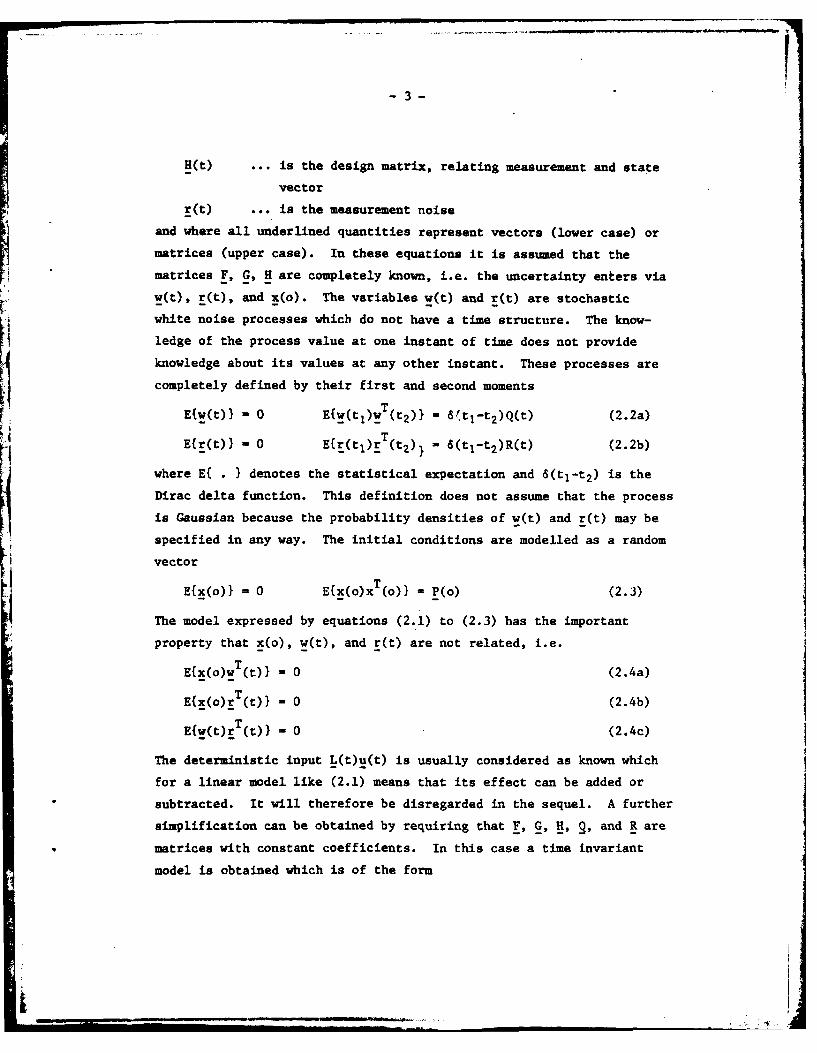
H(t) ... is the design matrix, relating measurement and state

vector

r(t) ... is the measurement noise

and where all underlined quantities represent vectors (lower case) or

matrices (upper case). In these equations it is assumed that the

matrices F, G, H are completely known, i.e. the uncertainty enters via

w(t), r(t), and x(o). The variables w(t) and r(t) are stochastic

white noise processes which do not have a time structure. The know-

ledge of the process value at one instant of time does not provide

knowledge about its values at any other instant. These processes are

completely defined by their first and second moments

E{w(t)} - 0 E{w(tl)wT(t2)) - :t-t2)Q(t) (2.2a)

E{r(t)} - 0 E{r(tl)rT(tz)} - 6(tj-t2)R(t) (2.2b)

where E{ . } denotes the statistical expectation and 6(tl-t 2) is the

Dirac delta function. This definition does not assume that the process

is Gaussian because the probability densities of w(t) and r(t) may bespecified in any way. The initial conditions are modelled as a random

vector

E{x(o)} - 0 Efx(o)x T(o)) = P(o) (2.3)

The model expressed by equations (2.1) to (2.3) has the important

property that x(o), w(t), and r(t) are not related, i.e.

E{x(o)w (t) - 0 (2.4a)

E{x(o)r (t)) - 0 (2.4b)

E{w(t)rT(01 - 0 (2.4c)

The deterministic input L(t)u(t) is usually considered as known which

for a linear model like (2.1) means that its effect can be added or

subtracted. It will therefore be disregarded in the sequel. A further

simplification can be obtained by requiring that F, G, H, 2, and R are

matrices with constant coefficients. In this case a time invariant

model is obtained which is of the form

L| _____________

-4-

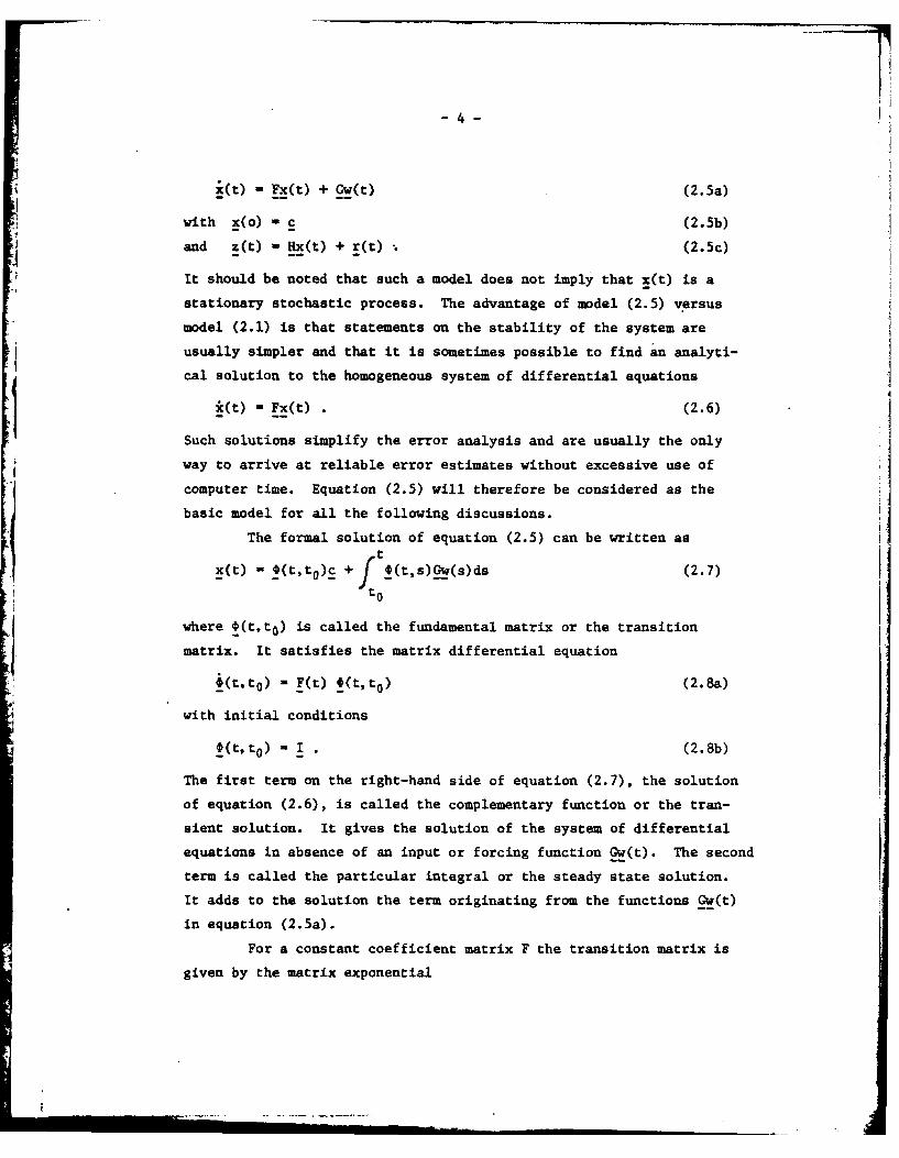
-Fx(t) + Gw(t) (2.5a)

with x(o) - c (2.5b)

and z(t) Hx(t) + r(t) . (2.5c)

It should be noted that such a model does not imply that x(t) is a

stationary stochastic process. The advantage of model (2.5) versus

model (2.1) is that statements on the stability of the system are

usually simpler and that it is sometimes possible to find an analyti-

cal solution to the homogeneous system of differential equations

(t) - F . (2.6)

Such solutions simplify the error analysis and are usually the only

way to arrive at reliable error estimates without excessive use of

computer time. Equation (2.5) will therefore be considered as the

basic model for all the following discussions.

The formal solution of equation (2.5) can be written ast

x(t) - 0(t,t 0 )c +f b(ts)Gw(s)ds (2.7)

to

where 0(t,t0 ) is called the fundamental matrix or the transition

matrix. It satisfies the matrix differential equation

i(t,t0 ) - F(t) 4(t,t 0) (2.8a)

with initial conditions

!(t,t 0 ) = I . (2.8b)

The first term on the right-hand side of equation (2.7), the solution

of equation (2.6), is called the complementary function or the tran-

sient solution. It gives the solution of the system of differential

equations in absence of an input or forcing function Gw(t). The second

term is called the particular integral or the steady state solution.

It adds to the solution the term originating from the functions Gw(t)

in equation (2.5a).

For a constant coefficient matrix F the transition matrix is

given by the matrix exponential

-5-

!(t,t o ) = e(t - to ) (2.9a)

or using the well-known series expansion of the exponential by

S(tto)i ! (2.9b)

!(t,t0 ) M (.b

Using the Cayley-Hamilton theorem the infinite series expansion can

be replaced by a finite series of order N where N is the rank of F.

A discussion of this approach and its usefulness in applications is

given in Biermann (1971). However, it is not always the most direct

way to a solution. Often the use of the Laplace transform is simpler.

The Laplace transform L of a function x(t) is defined as

f(s) L{x(t)) (2.10a)

f f-Stx(t)dt (2.10b)

0

where t> 0 and the integral converges for some value of s. Similarly,

for a vector x(t) of functions xi(t)

f(s) = L{x(t)}

fe-Stx(t)dt (2.11b)0

where the operation (2.10b) is now performed on each element of x(t).

Taking the Laplace transform of equation (2.6) results in

sf(s) - x(O) - F f(s) (2.12a)

and using (2.5b) we obtain

(sI - F) f(s) - c . (2.12b)

Thus, the system of differential equations (2.6) has been converted

into a system of algebraic equations. If the inverse of (sI - F)

exists we can write

f(s) - (SI - F)gc

-6

where the superscript g denotes some suitably defined inverse. In

the following, we will only use the Cayley inverse, thus obtaining

f(s) - (sI - F) -c . (2.12c)

Hochstadt (1975) discusses in detail the existence of the Cayley in-

verse for the above case.

The inverse Laplace transform L-1 reverses the operation (2.11),

i.e.

x(t) - L {f(s)} (2.13)

where the same symbols as in equation (2.11) have been used. The

functions x(t) and f(s) are often called a Laplace transform pair.

Thus, the solutions to the algebraic equations (2.12c) can be inverse

transformed to provide solutions to the original differential equa-

tions (2.6). This elegant and powerful technique will be frequently

used in the following and therefore a simple example will be given here

to demonstrate the salient features of the technique.

Consider the system of differential equations

=- -Kdv - w2 6p

6p = Sv

which is of type (2.6) with

We = , F = and c = [1 (2.14)

We thus have

s+K W2

(sI - F)-1 s

and its inverse

(s I - F)- 1- - s(s+K) + w2 [ s+K]

The individual components of f(s) are therefore

-7-

fs(s +K) + 2(s+K) +

c f (s) -cf (a)

1 K 1 2 12

ci (s+K)c 2

2(s) s(s+K) + w2 s(s+K) + w2

- cIf 2 1 (s) c 2f 2(S)

Due to the linearity property of the inverse Laplace transform we can

take the transforms of the individual terms. In a table of transform

pairs, as e.g. McCullum and Brown (1965) or Doetsch (1971), we can

find the inverse transform of f2 1(s)

21 s2(s+K) + 2

(2.15c)K

'-e 2 sin Dt x 21(t)D D

where 1) _ yl f: and D> 0. Using the same transform pair and

the linearity property we get

Ll f1(s) L l1 W2

S s(S+K) + w2}

(2. 15b)W2 - Kt

= - 2 sin D xt x1 2 (t)

Then we have

L-1 {f1 1 (s)} = L-1 {sf 21 (s)}

and using the formula

L-1 {sf(s)} - x'(t) + f(O)6()

S

8-

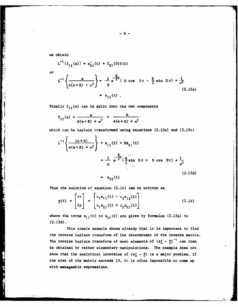
we obtain

L-1 f 11 (s)) X 1 (t) + f 2 1 (O)6(t)

orK

- { cos Dt- t sin Dt} +sis + K) +,,2 D

(2.15a)

- x 1 (t).

Finally f2 2(s) can be split into the two components

f (s) S + KS(s+K) + w2 s(s+K) + w2

which can be Laplace transformed using equations (2.15a) and (2.15c)

L- (s+ K) - x (t) + Kx (t)(s+K) w2J 1 i

K1 e E (sin Dt + D cos DO +

D 2

(2.15d)- x22(t)

Thus the solution of equation (2.14) can be written as

x(t) c1x11(t) - cX 12(t) (2.16)6p LciX 21(t) + c x22 (t)j

where the terms xl(tl to x 2(t) are given by formulas (2.15a) to(2.151).

This simple example shows already that it is important to find

the inverse Laplace transform of the determinant of the inverse matrix.

The inverse Laplace transform of most elements of (sI - F)--1 can then

be obtained by rather elementary manipulations. The example does not

show that the analytical inversion of (sI - F) is a major problem. If

the size of the matrix exceeds 10, it is often impossible to come up

with manageable expressions.

-9-

The basic model (2.5) is not always sufficient to cover all

cases encountered in practical problems. Two important extensions

are the modelling of coloured noise and nonlinearities in the basic

model. Time correlated noise processes will be used to model the

effect of the anomalous gravity field. The usual approach is by

state vector augmentation. The coloured noise wI is modelled as the

output of a linear system

- FwI + w3 (2.17)

where w3 is again white noise. This equation is added to equation

(2.5) resulting in

= + (2.18)

where w in equation (2.5) is defined by

S+1 W-2

and y2 is white noise. Because of equation (2.18) this is called state

vector augmentation. The assumption is that the correlated noise pro-

cescan indeed be modelled by (2.17). In theory, this is not always

possible. In practice, it can usually be done with sufficient accuracy.

In engineering applications the following F -matrices are often used:

F - ,w

modelling a first-order Markov process, and

rw 0

modelling a bias term. A more detailed discussion of suitable models

for the anomalous gravity field will be given in section 4.

Nonlinearities in the basic model will play no role in the

following and reference is therefore made to standard textbooks as

Gelb (1974) and Eykhoff (1974).

• .5 ' .:

- 10 -

3. ERROR PROPAGATION AND STEADY STATE ERRORS

There are two major practical advantages of using the dynamic

model (2.5). First, the real-time implementation of these formulas

including update measurements presents no problem. Kalman filtering

and its alternatives have been investigated in great detail and their

numerical characteristics are well-known. Second, a differential

equation for the error propagation can be derived from which an ex-

pression for the steady state error of individual states can be

obtained. The derivation of the basic error equation, the linear

variance equation, and its solution for the steady state errors will

be given in this section. The application of this technique to

derive analytical expressions for the position errors in airborne iner-

tial navigation will be given in section 5.

The statistical description of the total error of a dynamical

system at a certain time t is given by the covariance matrix P(t)

P(t) - E{x(t) x (t)1 . (3.1)

The change of P(t) with time models the error propagation. We will

thus consider the function P(t, t-)

P(t, t-e) - E{x(t) xT(t-)} (3.2)

where e is a small positive number, and then use limit arguments to

arrive at the result. Differentiation of equation (3.2) with respect

to time yields

i(t, t-e) - E{(t)x T(t-c) + x(t)T(t-e).

Using equation (2.5a) we obtain

P(t, t-e) - E{[Fx(t) + Gw(t)]x T(t-e) +

T T T Tx(t) T(t-c)F + w (t-c)GrlI

or

P(t, t-e) - E{Fx(t)x T(t-e) + Gw(t)x T(t-C) +

(t)T(t-C)FT + x(t)wT(t-c)GT} (3.3)

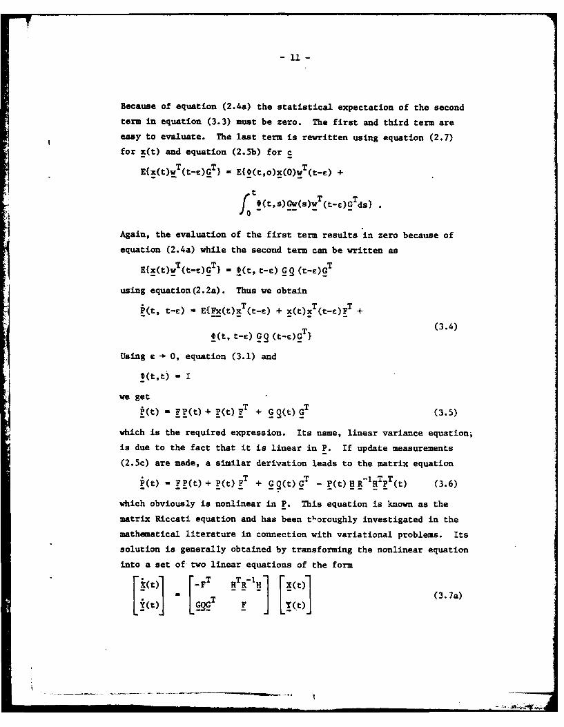
- 11 -

Because of equation (2.4a) the statistical expectation of the second

term in equation (3.3) must be zero. The first and third term are

easy to evaluate. The last term is rewritten using equation (2.7)

for x(t) and equation (2.5b) for c

E{x(t)w T(t-c)G I - E{_0(t,o)x(O)w T(t-C) +

tT TSto 0(t, s) Gw(s)!(t-c)G ds.

Again, the evaluation of the first term results in zero because of

equation (2.4a) while the second term can be written as

E(x(t)w7(t-e)GT ) - *(t, t-) G 9 (t-e)GT

using equation(2.2a). Thus we obtainT-T T

i(t, t-e) -E{Fx(t)x T(t-e) + x(t)x T(t-c)FT +T (3.4)

0(t, t-C) G0 (t-e)GT

Using c 1 0, equation (3.1) and

_*(t,t) - I

we get

P(t) - FP(t) + P(t) FT + G9(t) GT (3.5)

which is the required expression. Its name, linear variance equation,

is due to the fact that it is linear in P. If update measurements

(2.5c) are made, a similar derivation leads to the matrix equation

P(t) - FP(t) + P(t) FT + G2(t) GT - P(t) HRH TP T(t) (3.6)

which obviously is nonlinear in P. This equation is known as the

matrix Riccati equation and has been tloroughly investigated in the

mathematical literature in connection with variational problems. Its

solution is generally obtained by transforming the nonlinear equation

into a set of two linear equations of the form

-i(t)]" [_FT HTR- 1 (3.7a)

F Y t

-12-

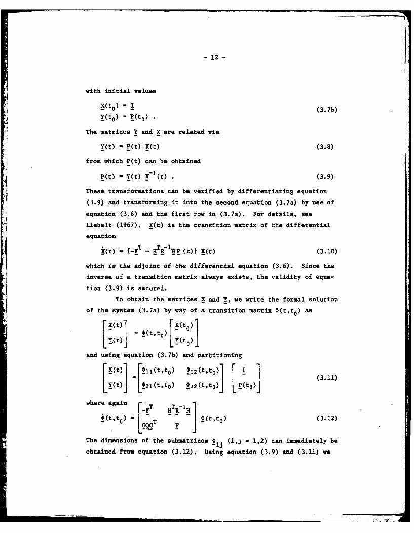
with initial values

X(t0) . I (3.7b)X(to) - t(to) •

The matrices Y and X are related via

Y(t) - P(t) X(t) .(3.8)

from which P(t) can be obtained

P(t) = Y(t) x-l(t) . (3.9)

These transformations can be verified by differentiating equation

(3.9) and transforming it into the second equation (3.7a) by use of

equation (3.6) and the first row in (3.7a). For details, see

Liebelt (1967). X(t) is the transition matrix of the differential

equation

X(t) - {-FT + TR7 H P (t)I X(t) (3.10)

which is the adjoint of the differential equation (3.6). Since the

inverse of a transition matrix always exists, the validity of equa-

tion (3.9) is secured.

To obtain the matrices X and Y, we write the formal solution

of the system (3.7a) by way of a transition matrix 0(t,t 0) as

1(t) [ t 1Y.(t) (tto) IYt O)

and using equation (3.7b) and partitioning

X(t) Fll(t,to) 012(t,to)

[(t)J bL2 1(t.to) 12 2(tto)j P(to)

where again FT HTRIH 1

(t .t0) 4(t,t0 ) (3.12)

The dimensions of the submatrices 9 j (i,j - 1,2) can immediately be

obtained from equation (3.12). Using equation (3.9) and (3.11) we

- 13 -

finally get the solution

P(t) - {21(t,t0)+ _2 2(t,t0)P(t0 ) {) 1 1(t,t0 )+ _12 (t,t0 )P(t0 )) (3.13)

which gives the covariance matrix P at an arbitrary time t in terms

of its initial values P(t0) and the transition matrices of the system

(3.7a). This solution goes back to Reid (1946). A proof and general

discussion is given in Levin (1959). Its first application to optimal

estimation problems can be found in Kalman and Bucy (1961).

The practical use of equation (3.13) is somewhat limited

because the transition matrices are seldom given in analytical form.

Usually, they are computed by numerical integration and in this case

recurrence relations are much more efficient to use. In our case,

however, equation (3.13) can be sufficiently simplified to obtain use-

ful analytical expressions. The first simplification is due to the

fact that we do not have to solve the general equation (3.6) but the

special case (3.5). Noting that

T R-1H - 0

and using the Laplace transform technique on equation (3.12), we

obtain

s!_T_! (t ,to) -I + T-1

-G _T ST -F

and after performing the matrix inversion

(sI + FT1>

!(t,t 0 ) - L-1 {[(3)1Gc(LFr.V~F.14)

and for the individual submatrices

-1-(t,t 0) - L- {(sI+ FT) - 1 (3.15a)

_1 2 (t,to) - 0 (3.15b)

- 14 -

!2 tt)-L {(sI- F)_ I9 ?(sI+F (3615c)

!22(t't0 ) - L-1 {(sI-FfI . (3.15d)

Furthermore, we are only interested in the steady state errors, i.e.

in that part of P(t) which is independent of P(t0 ). Thus, observing

equation (3.15b) and the steady state requirement, equation (3.13)

simplifies to

-1

P (t) - f2 1 (t,to) 011 (t,tO) . (3.16)

where the subscripts 'ss' denote the steady state solution. The matrix

identity

(sI+ F) - {sI+F)-1} T (3.17)

can be applied to show that

T-122(t,t0) - 011 (t,t0 ) (3.18)

and is also useful in simplifying the algebraic operations in (3.15c).

The diagonal terms of P will be used in section 5 to derive analy--sS

tical expressions for the steady state position error.

4. COVARILANCE MODELS FOR THE ANOMALOUS GRAVITY FIELD

- J In order to apply the error Analysis developed in the last

-j section, the effects of the anomalous gravity field have to be

modelled into a form compatible with equation (2.5). This requires,

first of all, that the characteristical features of the field can be

described in statistical language, e.g. in terms of random functions

and their associated covariance functions. The justification of such

an approach is given in Moritz (1980) and within the limits indicated

there, it is applicable to the following analysis. The second

requirement is the transformation of the position dependent covari-

ance function into a time dependent covariance function by way of the

velocity. As long as the velocity is constant and the basic co-

variance function isotropic, this transformation corresponds to a

simple "time-scaling" of distances between points. Since a constant

aircraft velocity is a reasonable assumption in our case, and since

all gravity anomaly covariance functions in practical use are iso-

tropic, this transformation does not present a problem. More impor-

tant for the model selection are two other requirements. One is that

the model is self-consistent, the other that it can be expressed by a

set of differential equations of the form (2.17). Self-consistency

means that the mathematical relationships which are known to exist

between the anomalous potential and linear functionals of it have to

be used when deriving the covariance functions of these quantities.

In other words, the covariance functions of the potential and the

covariance functions of its derivatives are not independent. In the

geodetic literature self-consistency with respect to the covariance

functions is usually discussed in the context of covariance propaga-

tion. The other requirement is obviously important whenever an error

model of type (2.5) is used. It has found considerable attention in

the navigation literature but has so far been neglected by geodesists.

For our analysis both aspects are equally important.

When comparing the resulting covariance models, two major

groups can be distinguished. They will be labeled 'geodetic' and

- 16 -

Inavigational' to indicate their predominant user groups. The

geodetic models are based on spherical approximation and are self-

consistent and global in character. Upward continuation of these

functions is no problem and the derivation of local models from the

global function is relatively simple. The important parameters of

these models are derived from different data groups, specifically

spherical harmonic coefficients obtained from satellite observations,

gravity anomalies and second-order gradients. Their major disadvan-

tage for an error analysis of this type is that there is no simple

way to express them in the form (2.17). A detailed discussion of the

mathematical structure of these functions is contained in Tscherning

(1976) and Moritz (1976). The fitting of a global function is

described in Tscherning and Rapp (1974) and Jekeli (1978) while localaspects are treated in Schwarz and Lachapelle (1980) and Lachapelle

and Schwarz (1980). Efficient numerical methods to compute the co-

variance function are treated in SUnkel (1979, 1980). Some modelling

aspects of nonhomogeueous global covariance functions are discussed

in Rummel and Schwarz (1977). The navigational models are based on

a flat earth approximation and are local in character. Their major

advantage is that they can be cast into the form (2.17), i.e. they

can be represented as the output of a linear system driven by white

noise. Not all of them are self-consistent and most of them cannot

be upward continued in a simple way. Usually the upward continuation

integral has to be evaluated. The extension of the local function to

a global function is in general not possible. The important parameters

of these functions are usually determined from one data group only,

specifically gravity anomalies or deflections of the vertical.

Levine and Gelb (1969) were the first to model deflections of the

vertical in this way. Subsequent contributions are due to Shaw et al

(1969), Vyskosil (1970), Grafarend (1971), Kasper (1971) but it was

especially Jordan (1972, 1973, 1981 et al) who in a series of papers

discussed both the geodetic and navigational aspects of different

models and synthesized the work of his predecessors.

- 17 -

This brief discussion shows already that for the airborne

case a combination of the two approaches is needed. On the one hand,

the geodetic model provides a simple procedure to compare different

approximations of the gravity field in a consistent manner and to

evaluate the effect of upward continuation. On the other hand, only

the navigational model can be used in a state space formulation which

forms the basis for the dynamic error model. All covariance functions

will therefore in the sequel be based on a consistent geodetic model

and only in the last step the transition to the navigational model

will be made. This last step cannot be'done rigorously but will

always involve an approximation. To keep approximation errors small,

the fitting of the navigational model will be done by way of the

essential parameters defined by Moritz (1976). Agreement of these

parameters for two models secures agreement of the error estimates

derived from them. The remainder of this section will review the

formulation of the geodetic model, define the essential parameters,

and discuss some simple navigational models which can be used as

approximations.

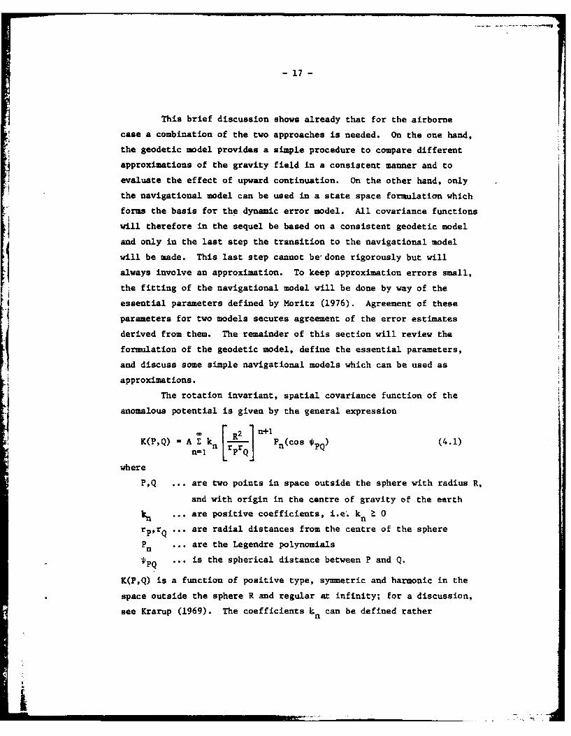
The rotation invariant, spatial covariance function of the

anomalous potential is given by the general expression

K(P,Q) - A E kn Pn(cos 1pQ) (4.1)

where

P,Q ... are two points in space outside the sphere with radius R,

and with origin in the centre of gravity of the earth

S... are positive coefficients, i.e. kn 0

rprQ ... are radial distances from the centre of the sphere

Pn ... are the Legendre polynomials

*pQ ... is the spherical distance between P and Q.

K(P,Q) is a function of positive type, symmetric and harmonic in the

space outside the sphere R and regular at infinity; for a discussion,

see Krarup (1969). The coefficients 4n can be defined rather

* I

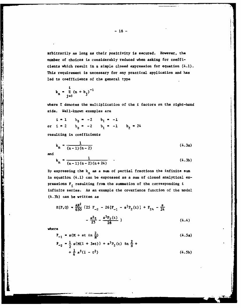
-18

arbitrarily as long as their positivity is secured. However, the

number of choices is considerably reduced when asking for coeffi-

cients which result in a simple closed expression for equation (4.1).

This requirement is necessary for any practical application and has

led to coefficients of the general type

k n (n+ b) 1

where H denotes the multiplication of the i factors on the right-hand

side. Well-known examples are

i = 1 b0 = -2 bi = -1

or i - 2 b0 = -2 bI = -1 b2 24

resulting in coefficients

n - 1) (n- 2) (4.3a)

a d k = -(4.3b)

n (n- 1) (n- 2) (n+ 24)

By expressing the kn as a sum of partial fractions the infinite sum

in equation (4.1) can be expressed as a sum of closed analytical ex-

pressions Fi resulting from the summation of the corresponding i

infinite series. As an example the covariance function of the model

(4.3b) can be written as

K(P,Q) = - {25 F_ - 26F_ - s 3 P2(t)] + F650 -2 -1 2 t) + 24 24

s2t s 1(t) (4.4)

25 26

where

F 1 s(M + st in 2 (4.5a)

F 2 = 1 s{M(l + 3st)) + s3p2(t) Zn 2 +

+ s3(l - t2) (4.5b)

I1

-19

and F2 can be computed from the recursion formula

Fk+l - 1 {L + (2k-l)tFk - (k-l)s-Fk_ } . (4.5c)

The auxiliary quantities L,M,N are defined by

L - {1 - 2st + s2}

M- 1-L-st

N- l+L-st

where

t - cos *pnR2

rr

PQ

and A and P2 (t) have been defined earlier. For a detailed derivation

reference is made to Tscherning and Rapp (1974). Expressions of the

form (4.5a) to (4.5c) are easy to evaluate on a computer and are

simple enough to allow the formation of all derivatives necessary for

covariance propagation. Thus, the basic model given by equations

(4.1) and (4.2) is used to derive a self-consistent set of covariance

functions for functionals of the anomalous potential. These deriva-

tions are given in Tscherning and Rapp (1974) and Tscherning (1976)

for a number of different models.

To obtain a satisfactory fit of empirically determined data to

equation (4.1), the following variables can be changed:

the size of A

the radius of the sphere R

the coefficients kn according to one of the models (4.2).

The effect of a change in the first variable is simply that of a

scaling factor for all coefficients and thus for the total covariance

function. It is directly related to the variance K(O,O) or the

derived variance of the gravity anomaly C(0,O) which can be easily

determined from given point gravity anomalies. A change of R affects

the spectrum of K(P,Q) in a non-uniform way. For instance, a decrease

of R works similar to a low pass filter by strongly damping the

-20-

- I higher frequencies. Similarly, when going from model (4.3a) to

model (4.3b) a damping of the high degree terms will be the result.

It is therefore important to ensure that a covariance function of

type (4.1) fits well to data representing different parts of the

spectrum. Typically, geoidal undulations or geopotential models

from satellite observations contain mainly low frequency information

while torsion balance measurements or gradiometer data represent the

high frequency range. Gravity anomalies and deflections of the

vertical take an intermediate position containing mostly information

on the medium frequency range. At present it appears that a model

of type (4.3b) or a combination of this model with one of a simpler

structure gives the best fit to all available data. It was therefore

decided to use model (4.3b) for the following computations. Once the

basic structure of the model is given, we have to specify what will

be understood by goodness of f it. For instance, is it important to

approximate an empirical covariance function as closely as possibleeverywhere or are certain regions especially important? Or, should

empirical degree variances computed from satellite solutions replace

the low order {Akn} in equation (4.1)? Questions of this type have

been answered by Moritz (1976, 1977) in a discussion of the essential

parameters of planar covariance functions. These functions can be

considered as planar equivalents of the covariance functions (4.1)

and results obtained for them carry over to the spherical case with

only small modifications.

Moritz (1976) defines three essential parameters for co-

variance functions of this type: the variance Ko, the correlation

length t, and the curvature parameter X. The variance K 0 is the

value of the covariance function K(*p) for the argument q0, i.e.

K0 K(O) (4.6a)

The correlation length is the value of the argument for which

K( ) -1 K(4.6b)2~ K0

- 21 -

The curvature parameter X is related to the curvature K of K(O) at0 by

X= K • C2/ 0 (4.6c)x0

where K is given in the usual way by

K" (4.7)

(1 + K,2)3/2

and2K a2K

K'-- K" -ap a02

with

p - R .

Usually, the fit is made to empirical values of the gravity anomaly

covariance function C(*) because large data samples are available.

In this case, the curvature K is equal to GO , the variance of the

horizontal gradients of Ag. Thus we have

X = G0 2 / CO ; (4.8)

for.a derivation see Moritz (1976). In this case all three essential

parameters can be determined from actual measurements. C0 is the

global variance of the gravity anomalies; 4 is the correlation length

of the empirical covariance function C(i) which can be determined

graphically; Go can be computed either from dense point gravity anoma-

lies or from torsion balance or gradiometer measurements. For a

more detailed discussion, see Schwarz and Lachapelle (1980).

Two cc,-ariance functions which have the same essential para-

meters are not necessarily equal everywhere. However, their general

behaviour with respect to interpolation will be similar. This is

obviously a very important property for the analysis in this report.

It can also be shown that the shape of the covariance curve at dis-

tances larger than about 1.5 does not influence the interpolation

very much. This is quite important for any empirical covariance

fitting.

Besides relating the covariance model (4.1) to the actual

data, the set of essential parameters can also be used to get a good

-22-

fit between the geodetic and the navigational models. This will be

the main application in the following. Covariance functions for the

deflections of the vertical will be derived from the best available

71 model (4.1). Upward continuation in this model requires only a change

of rp and rQ. Improved gravity models can be simulated by subtract-

ing a certain number of low degree coefficients from the series. By

basing all computations on one fundamental model of type (4.1), self-

consistency between different functionals of T as well as consistency

between the different cases is secured. By defining each covariance

function in terms of its essential parameters, self-consistency of

the approximating navigational model is not required anymore. Emphasis

will therefore be on selecting navigational models which give a best

fit in terms of essential parameters for the individual covariance

* functions.

The navigational covariance models most frequently used are

low-order Gauss-Markov models whose covariance functions are of the

general form (Gelb, 1974)

-'n n-I r(n)(2nI)n-k-1

K(t) W a2 e-' 1 Z + m2 (4.9)n k-0 (2n- 2)! k i r(n- k) n

whereCt2 ... is the variance of the processn

n ... is a parameter related to the correlation length

m .. is the mean

r(n) ... is the Gamma function

n ... is the order of the Gauss-Markov process

and Irj is the independent variable, i.e. distance in geodetic appli-

cations and time in navigation applications. Implicit in this defi-

nition is that the process is stationary and its probability density

function is Gaussian. Processes of this type are defined by a

stochastic differential equation of order n or equivalently by a

set of n first-order stochastic differential equations. They are

- 23 -

therefore convenient to use in our problem.

The covariance function of the first-order Gauss-Markov

process is the simple exponential function

K() a2 e + .2 (4.10)

The process is defined by the differential equation

x+ x - w (4.11)

where w is white noise. Because of its simplicity, this process is

often used to model physical phenomena. It is not a consistent model

with respect to the gravity field. But since consistency is provided

by the geodetic model this is not a major concern. The essential

parameters of this process are

1 1 1 0.693In- I 6 4.12a)

X1=(in 2)2 =0.490

It should be noted that in the navigational literature the correlation

distance C is used instead of C . It is defined as1

K( ) = 1 K0 (4.13)

where e is the basis of the natural logarithm. In order to differen-

tiate between C and Z without too much verbal acrobatics we will

continue to call C the correlation length while Z will be called the

correlation distance. For the above case

- 1 (4.12b)

The covariance function of the second-order Gauss-Markov

process is given by

K(T) - am{+ $ 2 j T e2 1 1 + M2 . (4.14)

- 24 -

The corresponding differential equation is of the form

x + 280 4B (4.15)- 2-"2- -

The essential parameters are

2

1.6782 82 (4.16)

2.146

X2 2.817

where c2 is obtained by solving the equation

tn(1 + 02;2) - 02C2 - 1

and 42 by solving

tn(l + B2C2) - 02 2 - Zn 2

Similarly, the covariance function of the third-order Gauss-

Harkov process is given by

K(T) - 32 {1 + 83 1, 1 + 2 It1) e83(T) + . (4.17)

with the corresponding differential equation

+30 3 j +30 2 +a 3 x w (4.18)

and the essential parameters

K0 -' 32

2.330C3 3 (4.19)

3 .2.903C3 03X 3

x3- 1.810

-25-

The correlation distance is computed by solving

i (I1++ ) " -383 1

and the correlation length C by solving

(1 + 1 2 2 -. n 2.An 3 +83 3 ~3 3 3 C 3

Both the second and the third-order Gauss-Markov models are self-

consistent models for the representation of the anomalous gravity

field. Jordan (1972) advocates the third-order model for the

anomalous potential because it results in a gravity anomaly covari-

ance function with a realistic behaviour at * - 0 or T - 0 respec-

tively. As mentioned above, self-consistency of the navigational

model is not a major concern in our case. The selection of an

appropriate model should therefore be based on the agreement between

the essential parameters of the geodetic model and the navigational

model. Equations (4.12a), (4.16) and (4.19) show that variance and

correlation length are variable while the curvature parameter is

constant. This means that any parameters K0,,;, required by the

geodetic model, can be accommodated by the navigational model. The

selection of an optimal fit can therefore be done on the basis of

X only. In our case the curvature parameters of the deflection

covariance functions C(C,E) and C(n,) are required. They can be

derived from equation (4.1) by using the well known relations

1 aTry 3f

n 1 3Try cos 35

to obtain

cov( Q& 1 32K(P,Q) (4.20a)Q r rQ p YQ 3¢p ¢ao

1

-26-

cov(npr 1 1 a2K(P,Q) (4.20b)Q)- rprQ coo Q Yp YQ aXp axQ

The differentiations of K(P,Q) can be done by using

cOS*pQ = Sip sin*Q + cOS p COSOQ COS(XQ-X_)

and formulas (4.4) and (4.5). Then introducing again planar approxi-

mation, a double differentiation of the functions (4.20) with respect

to p will give K and thus X. To avoid the cumbersome differentia-

tions, it has been assumed that the curvature parameter of the gravity

anomaly covariance functions is close enough to the corresponding

parameter of the deflection covariance function. Thus, equation

(4.8) has been used. The actual computation and comparison of these

parameters is given in section 6.

- 27 -

5. THE STEADY STATE POSITION ERROR INDUCED BY GRAVITY FIELDAPPROXIMATIONS

The procedure outlined in section 3 led to the formula

-sst !2 1 (tto) 01 1 (t,to) (3.16)

for the steady state errors of a linear system. Using equation (3.18)

this can be rewritten as_ 0T

Ps(t) - 02 1 (t,to) 22 (t,to) (5.1)

To obtain 4he steady state position errors induced by different gravity

field approximations, the system of differential equations for this

problem has to be set up. For a three-axes inertial navigation system

the minimum system is of order 12 containing the following elements in

the state vectorT

- N' LE, cD9 6PN' TPE' (PDC VN, svE' 6p 6vD' n, SN) (5.2)

where the subscripts N, E, D denote the directions of the three axes

of a local-level system (North, East, Down) and

C ... are attitude errors

6p ... are position errors

6v ... are velocity errors

, ... are the deflections of the vertical in north and east

direction

SN ... is the geoidal undulation.

The dynamics matrix for the first nine states can be found in Britting

(1971) while for the states representing the anomalous gravity field

one of the models in section 4 can be used. The solution of this

system applying Laplace transform techniques is a formidable task. To

give an idea of the type of analytical "anipulations necessary, refer-

ence is made to Wong and Schwarz (1979) where the transition matrix

!22 has been derived for the first 9 states in equation (5.2). Con-

sidering that the three additional states will complicate the deriva-

tion considerably and that the determination of 021 is much more

complicated than that of 022, it was decided to consider only the

- 28 -

single axis case, i.e. to completely decouple the three channels.

*1 Results obtained from numerical integration techniques indicate that

this simplified case represents the error behaviour of the more

general model quite well. Thus results obtained in this way will in

general be also valid for the more extensive model. The obvious

advantage is that a much smaller system has to be dealt with. This

is probably the main reason why all previous investigations followed

this route.

The single axis case for one of the horizontal channels is

given by the differential equations

6I - -K6v - w26p - y (5.3a)

6p - 6v (5.3b)

= - 1C + u (5.3c)

where

y ... is normal gravity which for this error analysis can always

be replaced by

G ... the global mean value of gravity,

w ... is the Schuler frequency

where fG)-w G (5.4)

R ... is the mean radius of the earth

K ... is the feedback gain which is related to

d ... the loop damping parameter by

K - 2dw , (5.5)5

is the deflection of the vertical (either or n)

and u, ... is white noise defined by

E{ul(t) ul(T)l = qS(t-T) (5.6)

where the power density spectrum in case of equation (5.3c) is given

by

q, = 201 a2 (5.7a)

and 01 and a are defined as in equation (4.10). The power density

- 29 -

spectrum for the second and third order Gauss-Markov process are

given by

48 3 o2 (5.7b)

and q 160 5 a2 (5.7c)13B3 3

respectively. It should be noted that errorless velocity measurementshave been assumed to avoid a mixing of error sources for the position-

ing error.

Putting equations (5.3) into the standard form (2.5) we have

SV -K _W2 -G

6P [ 1 0 01

G- 0 0 01

ul 0 0 1

Thus

[s+K 2 G

(sI - F) -1 s 0

0 0 s+O

where the index of 8 has been omitted since no confusion is possible.

Inversion of this matrix results in

s/E1 -W2/E 1 -Gs/(s+ V)E,(S( - F s(s +)E I (5.8a)

0 1/(s+O) Jwhere

E s2 + sK + W2 . (5.8b)

Using equations (3.15d) and (3.18) we get

!22 (t,to) L-1 ((st-F)- 1 - L-1(B) (5.9)

which gives us one of the required components in equation (5.1). To

obtain 0_21 we have first to form the matrix product

- 30 -

- (sI-F)- 1 GG 2T (sI+ FT) - l

which is of the following form

$G2 s 2 8G2s Gs

(s 2 -0 2 )EIE2 (s 2 -0 2 )EIE 2 (s2-82)E1

- 202 - BG2s _ _ _ - (5.10a)(s 2 -82 )EE 2 (s2-02)E E2 (s2-82)E*1~s - ______2_1_2 1OGs OG 1

(s2-.2) E2 (s2-B2) E2 (s2-82)

where

E2 s2 - sK + w2 (5.10b)

and Elis again defined by equation (5.8b). 021 is then obtained by

the inverse Laplace transformK!21(ts0) C XI_A} = 202 Li{ b (5.11)

where A is the matrix on the right-hand side of equation (5.10a). The

steady-state position error is determined by the second diagonal ele-

ment in the P --mtrix (5.1). Using the individual elements of the

matrices A and B defined by equations (5.11) and (5.9) and the lin-

earity property of the Laplace transform, we can write the variance

a 2 of the position error in terms of inverse Laplace transforms

a2 2 [L-{a 2 1}L' {b2 1} + L-1fa22 }L- {b2 2)P (5.12)

+ L -{a 2 3 }L-1{b 23)]

The determination of the individual terms in equation (5.12) is most

simply accomplished by using the complex inversion formula

X(t) 1 f f(s) de (5.132wi ii

. ... In - . , , i , ' -t, •..

- 31 -

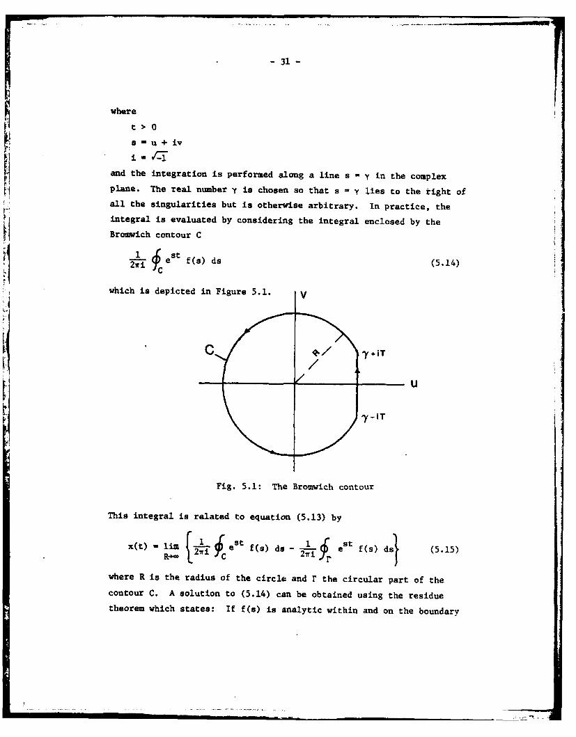
where

t> 0

S-U + iv

and the integration is performed along a line s - y in the complex

plane. The real number y is chosen so that s = y lies to the right ofall the singularities but is otherwise arbitrary. In practice, the

integral is evaluated by considering the integral enclosed by the

Bromwich contour C

ei f(s) ds (5.14)

hich is depicted in Figure 5.1. V

ly iT

Fig. 5.1: The Bromwich contour

This integral is related to equation (5.13) by

x(t) - li [ est f(s) ds -- Lf est f(s) d (5.15)

where R is the radius of the circle and r the circular part of thecontour C. A solution to (5.14) can be obtained using the residue

theorem which states: If f(s) is analytic within and on the boundary

- 32 -

of C of a region except at a finite number of poles pj within the

region having residues p_j respectively, then

# f(s) ds - 2vi E (5.16)

i.e. the solution can be obtained by determining the residues of f(s)

at the poles pj. They can be found by the general formula

W lim 1 dn-I f(s)) (5.17)s- li (n-i)! dsn

where n is the order of the pole. For simple poles equation (5.17)

reduces to

p-i = lim {(s-Pj) f(s)) . (5.18)

Replacing f(s) by es t f(s) and assuming

lim I est f(s) ds - 0 (5.19)

the solution of equation (5.15) can be written as

x(t) - E P.j (5.20)j

where p_j are the residues of est f(s) at poles of f(s). Sufficientconditions under which equation (5.19) is correct are e.g. given in

Doetsch (1971).

Returning to equation (5.12) we start with the first term

C a211 f (s2-2)

(s2-02)(s2:sK+W.2)(s.-sK+W2)}

El and E2 can be factored into

E, - (s+a) (s+b) (5.21)

E2 - (s-a) (s-b)

-33-

wherea - 1-K - K2 _ -2

2u ~~ 1 4(5.22a)

1 /12"

b - -K + IK2 - 22 4

Because d < 1 in equation (5.5) we get the complex roots

a - K - iD2 (5.22b)

b-K + iD

whereeD - (5.22c)

4

is now always positive. Using (5.21), we can write the inverse

Laplace transform of a21 as

L1{a2l)-1 BG2S

(s2-O2)(s2-a2)(s2-b2)

Thus, in this case the function f(s) has the six simple poles-±O, -±a, -.b. Using equations (5.20) and (5.18) we obtain

x21(t ) - L-1 {a,),)

S-'8 (S-s+8(-a)(s2-b2) I+ lim - 8G2 s est

S -a (S-S) (s2-a 2 ) (s2-b2)J

+ lim - BG2s est I

S -a (s2 82) (s-a) (s2-b2)J

lim G2s est8"s-a (S2-8 2 ) (s-a) (s2-b 2 )

+ JimGWs es t

&+ -b (s2-82)(s2-a2)(s-b)

s+b (s2-8 2)(s2 -a2 )(s+b)

__ _ __ _ _ __ _ __ _ _

-34-

Evaluating these expressions leads to

L-l{a21 - -G 2 coph t + cos h atS(2-a2)(B2-b2) (a2 -82) (a2-b2) (

~(5.23a)

+ cos h bt

(b2 -02 )(b 2 -a 2 ) JA check of this result can be obtained by splitting a21 into

a2 l(s) - fl(s) * f2 (S)

wheref(s) =

(s2-a2)(S2-b2 )

f2(s) - S -a

finding the inverse Laplace transforms xI(t) and x2(t) from a table

and applying the convolution theorem

x21 (t) x1 (t) * x2 (t)

XI (T) x(t-T) dr

This is, however, a more laborious procedure.

The next term, the inverse Laplace transform of a22 can be

obtained by observing that

L 1 {a} L 1 a122 { 21

Since in general

f(s)} f )

0

where x(t) is the inverse transform of f(s), we have in our case-,t

L {a22 1m-O x2 1(T) dT

0

35

-I where x2 1(t) is given by the right-hand side of equation (5.23a). The

integrals are simple to evaluate resulting in

L- {a SG2 sin h Bt + sin h at22 ( 2-a2) ( 2-b2) a(a2-B2) (a2-b2)

(5.2 3b)

+ sin h bt

b(b2-B2 )(b2-a2)

A check is again possible by use of the complex inversion formula and

the residue theorem. Applying similar techr~iques for the other four

terms, we obtain

L-1 {a2 ( a+B) cosh Bt-(a2-02) (b2-02)

(B2+ab) sinh Bt (a2 _82) e-btI } + (5.23c)

B (a-b)

(b2-82) e

-at

~a-b

C 1- {b 2 - e sin Dt, (5.23d)

compare equation (2.15c),

and The-Kt inDt +z: t a sn h (5.23e)

-l{b22} ue t K s t (5.23e)and C {b2 3 } I . - Ge a + e - t + e B (5 .23 f)

(b-)(Ba) (a-b) (8-b) (a-S) (b-8)

The variance of the position error can now be obtained by performing

the multiplications in formula (5.12) using the expressions (5.23a) to

(5.23f). The somewhat lengthy formula is not written out here. It

gives the steady state error as a function of time. Often we are only

interested in the behaviour of the error after it has settled down,

i.e. for t ®. The relevant expressions have been published by

-36-

several authors, see e.g. Jordan (1973), and are not rederived here.

They are usually obtained by applying the final value theorem of

Laplace transforms directly to equation (5.12).

For the first-order Gauss-Markov model with the covariance

function (4.10) we obtain

a2 l W r 2 G2 K + (5.24)P 1=2 (02 +KS + W2)

For the second-order Gauss-Markov model with the covariance function

(4.14) we get

+y2 2 G2 28 2(K+ 8 2) 2 + W2

a2 a2 -. (5.25)CP2 =C2 Kw 2 (a2 + KB 2 + W2) 2 (525

P2 2

Finally, use of the third-order Gauss-Markov model with covariance

function (4.17) results in

2G 2 W2 (MK2 + 3 11K2 + KW2 + 5 6 1 ) + 2 ( a 3+ K) 3

a2 =f a 3 2 -3 (5.26)P3 3 Kwn2 (0 2 + KO3+ W2)3

Equations (5.24) to (5.26) show that the elimination of time fromthe error function results in a considerable simplification of the

expressions. When comparing the effect of different gravity fieldapproximations we are primarily interested in the average behaviour

of the error over long time intervals. Thus, equations (5.24) to

(5.26) will serve our purpose well and will therefore be used in thenext section.

The discussion so far has been restricted to the two hori-

zontal channels, i.e. only the position errors due to unmodelled

deflections of the vertical have been considered. Formulas for the

height error due to unmodelled gravity anomalies or geoidal undula-

tions can be derived in an analogous way. They can for instance be

found in Jordan (1973). Due to the fact that the natural frequency of

the vertical channel is higher, these errors are much smaller, usually

less than 5% of those generated in the horizontal channels. They are

therefore not given here.

- 37-

The same procedure which was used to derive the steady state

position error can be employed to determine the steady state velocity

error induced by insufficient deflection information. In this case,

the first diagonal term of the P ss-matrix contains all the necessary

information. Formulas can be found in Levine and Gelb (1969) andJordan (1973).

-I-

4=

-38-

6. RESULTS

To use the formulas developed in the last section, three

j steps are necessary. First, the different gravity field approxi-

mations have to be specified using the geodetic model described in

section 4. Second, the essential parameters of the resulting co-

variance functions have to be determined. Finally, a suitable navi-

gational covariance model must be selected by fitting the essential

* parameters of the geodetic model to those of the navigational model.

After that, formulas (5.24) to (5.26) can be used to determine the

position error induced by insufficient knowledge of the deflections

of the vertical.

Gravity field approximations of increasing accuracy can be

represented by spherical harmonic expansions of increasing degree

and order N. When using such models in an airborne inertial navigator,

the long wave-length features of the gravity field are eliminated.

This means that with increasing N the unmodelled effects become more

and more local in character. The covariance representation of geo-

potential models of arbitrary degree and order N can be simulated by

subtracting the first N coefficients from the model (4.1). Covari-I ance computations with such models are done in exactly the same way

as with the full model. We thus have a consistent and simple way to

characterize different gravity field approximations.

Table 6.1 lists the models used in the following computations

and indicates reasons for their choice. The first three models

represent gravity field approximations available today. The next

three will hopefully become available on a global scale in the not too

distant future. The last two represent models of well surveyed areas

but cannot be considered as given globally. Since gravity field infor-

mation is often given in gridded form, the grid interval corresponding

to a geopotential model of degree and order N is also listed in the

last column. It has been computed by the approximate formula

grid interval - IN

which is useful for discrete function values but has limitations when

- 39 -

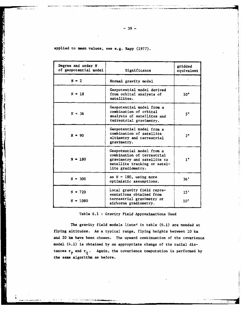
applied to mean values, see e.g. Rapp (1977).

Degree and order N griddedof geopotential model Significance equivalent

N - 2 Normal gravity model

Geopotential model derivedN 18 from orbital analysis of 100

satellites.

Geopotential model from acombination of orbitalanalysis of satellites andterrestrial gravimetry.

Geopotential model from acombination of satellitealtimetry and terrestrial

gravimetry.

Geopotential model from acombination of terrestrial

180 gravimetry and satellite to 1

satellite tracking or satel-lite gradiometry.

N 300 as N = 180, using more 36'optimistic assumptions. 3

N = 720 Local gravity field repre- 15'sentations obtained from

N - 1080 terrestrial gravimetry or 10'airborne gradiometry.

Table 6.1 Gravity Field Approximations Used

The gravity field models liste4 in table (6.1) are needed at

flying altitudes. As a typical range, flying heights between 10 km

and 20 km have been chosen. The upward continuation of the covariance

model (4.1) is obtained by an appropriate change of the radial dis-

tances rp and rQ. Again, the covariance computation is performed by

the same algorithm as before.

I -0-40-

The basic covariance model used to compute the models in

table 6.1 has the p .ameters

A - 607.57 mgal2

=1 (6.1)n~ (n-i)(n-2)(n+24)

s - 0.998444

where

and RM rp = rQ - 6371 km

is the mean radius of the earth. As usual, the parameter A corres-

ponds to the gravity anomaly covariance function. Its essential

parameters are

C - 1762 mgal20

- 48!4

X - 13.7

They correspond somewhat better to the observational data than the

parameters given by Tscherning and Rapp (1974). For a discussion,

see Schwarz and Lachapelle (1980).

The different models in table 6.1 were computed using the

subroutines COVAX by Tscherning (1976) and COVAPP by S6nkel (1979).

A graphic representation of the results is given in figures 6.1 to

6.4. They show the covariance functions for the two deflection com-

ponents at altitudes h - 10 km and h - 20 km. The gravity field

approximation is characterized by the degree and order N of the geo-

potential model. The covariance functions N > 180 for h - 10 km and

N > 90 for h - 20 km are too small to be represented in the given

scale.

Three distinct features can be observed from these graphs.

First of all, the covariance function of the n-component is much

smoother than that of the C-component (note that the scales of the

-41

COVARANCEitQ AT "' 1km

...... .............................

NN32

NIIS

rig. 6.2 Deflection covaance function Coo,)

at h 10 km

-42-

30-COVARIANCE ~ lAT h=20 km

0

0 o100 1&0O 200arc min(o4)

Fig. 6.3 Deflection covariance function C(&,E) at h -20 km

30- COV.ARIANCE[17,1] AT hrn20km

N UI0

so ISO15 200arc min(V')

Fig. 6.4 Deflection covariance function CQn,1i) at h -20 km

- 43 -

*-axis are different between the two sets of figures). This means

that we can expect a major difference in the correlation length.

Second, the effect of increasing the degree and order N of the approxi-

mation is a reduction of both the variance and the correlation length

of -the covariance function. This feature is easily explained because

the gravity field represented by the covariance function becomos more

and more local with increasing N. Finally, the effect of upward

continuation is a decrease in the variance but an increase in the

correlation length. Again, this is physically meaningful because the

high frequency spectrum is more affected by the attenuation with

height. It should be noted that these results cannot be generalized

to other functionals of the anomalous potential, as e.g. the geoidal

undulations or second-order gradients. Since they are influenced by

different parts of the spectrum their characteristical behaviour with

respect to changes in N and h is quite different. For a discussion

of this point, see Schwarz (1981).

The second step to the use of equations (5.24) to (5.26) is

the determination of the essential parameters for all covariance

functions. They can be obtained by applying the formulas of section 4

to the output of the subroutines mentioned above. Results are summar-

ized in tables 6.2 to 6.5 which correspond to figures 6.1 to 6.4.

Besides the features already mentioned, the change in the

curvature parameters X is of specific interest. It decreases with

increasing N and increasing h. Since the decrease with N is especially

pronounced for the first few degrees, all models with N 1 18 are quite

well represented by covariance functions of second and third order

Gauss-Markov models. This is an important result because it secures

a good fit of the geodetic to the navigational models. It should be

noted, however, that this is not true any more for inertial navigation

on the surface of the earth. Due to the increase of X with decreasing

h, the curvature parameters tend to be too large for low-order Gauss-

Markov models. That this is not a feature of the specific geodetic

covariance model used can be gathered from a table of empirically

7

- 44 -

odel Variance Correlation CurvatureN (arie C) length C distance 4 parameterN (arc sec)2 (arc min) (arc min) x

2 32.5 81.2 136. 7.41

18 19.8 40.3 54.2 3.9436 14.9 30.5 38.9 3.00

90 7.94 19.3 23.3 1.87180 3.57 12.7 14.9 1.48300 1.47 9.03 10.5 1.32

720 0.106 4.61 5.29 1.201080 0.0137 3.27 3.75 1.23

Table 6.2 Essential Parameters of DeflectionCovariance Function C(t,t) for h 1 10 km

Model Variance Correlation CurvatureN (arc e length c distance C parameterN = (arc sec)2 (arc min) (arc min) x

2 32.5 211. 387. 7.4118 19.8 92.0 132. 3.9436 14.9 66.4 89.9 3.00

90 7.94 39.2 49.7 1.87180 3.57 24.7 30.2 1.48300 1.47 17.1 20.5 1.32

720 0.106 8.51 10.0 1.201080 0.0137 6.00 7.05 1.23

Table 6.3 Essential Parameters of DeflectionCovariance Function C(no) for h - 10 km

- 45 -

Model Variance Correlat ion Curvaturelength C distance C parameter

N - (arc sec)2 (arc min) (arc min) Xix

2 27.0 113. 182. 6.5018 14.6 52.5 67.8 3.0236 10.1 38.8 47.9 2.22

90 4.35 23.5 27.8 1.57180 1.42 15.0 17.3 1.32300 0.390 10.3 11.8 1.24

720 0.00714 4.94 5.69 1.171080 0.000300 3.50 4.00 1.16

Table 6.4 Essential Parameters of DeflectionCovariance Function C(E,E) for h 20 km

Model Variance Correlation Curvaturelength distance C parameter

N- (arc sec)2 (arc min) (arc min) x

2 27.0 290. 511. 6.5018 14.6 116. 159. 3.0236 10.1 81.3 106. 2.22

90 4.35 46.2 57.1 1.57180 1.42 28.3 34.0 1.32300 0.390 19.1 22.6 1.24

720 0.00714 9.14 10.7 1.171080 0.000300 6.30 7.50 1.16

Table 6.5 : Essential Parameters of DeflectionCovariance Function C(nn) for h - 20 km

- 46 -

determined X-values published in Schwarz and Lachapelle (1980). They

have an average eize of X - 9 when referenced to a geopotential model

of degree and order 22. This means that at h - 0 the simple naviga-

tional models, which typically have x-values below 3, represent only

local disturbances of the anomalous gravity field well. They will

therefore give reliable estimates only when used with a gravity field

approximation of high degree and order. Since, at present, geopoten-

tial models with a large enough N are not available, navigational

models are needed which admit a larger curvature parameter. It is

also interesting to note that for the same reason the covariance

function of the first-order Gauss-Markov process is not a good model

of the anomalous gravity field anywhere in the range 0 h S 20 km.

The third step to the use of equations (5.24) to (5.26) is the

fitting of the geodetic models to one of the navigational models by

way of the essential parameters. This amounts to obtaining a good fit

for the curvature parameter because the variance and the correlation

length of the two models can always be made to agree. Using the geo-

detic model parameters given in tables (6.2) to (6.5) a second or

third order Gauss-Markov process is chosen depending on whether the

x-parameter in formula (4.16) or (4.19) is closer. Then, transforming

C into the time domain by

a, = =(6.2)i

where v is the aircraft velocity, formula (5.25) or (5.26) can directly

be applied. For a definition of terms in these equations, see formulas

(5.3) to (5.5). A damping factor of 0.3 has been used throughout.

Results for aircraft velocities of 300 knots, 500 "knots, and

800 knots are presented in tables 6.6 and 6.7. They show clearly that

the single most influential factor for a reduction of position errors

is the degree of the gravity field approximation model. Flying alti-

tude, aircraft velocity, and correlation distance have some effect but

are not decisive. Using one of the available geopotential models of

degree and order 36 instead of the normal gravity field would reduce

the errors by about 40% on average, and by 50% in case of a high speed

47

'I

Steady-state position error ap induced by

C(C,)l C(n,n) C(&,E) and C(n,n)Model 300kn 500kn 800ka 300ku 500km 800kna 300kn 500kn 800kn4-i N= (in) (n) (n) () (i) () (in) (in) (m)

2 197 208 207 180 186 195 267 279 28418 162 149 128 154 162 161 224 220 20636 135 117 98 140 141 131 194 183 131

90 69 53 41 97 78 61 119 94 73180 1 37 28 22 53 41 32 65 50 39300 19 15 12 28 21 17 34 23 21

720 4 3 3 5 4 3 6 5 41080 2 1 1 2 2 1 2 1

Table 6.6 Gravity Induced Position Error for h 10 km

Steady-state position error a induced by

i!Model 300kn 500kn 800 kn 300 ka 500 ka 800 kn 300 kn 500 kn 800 knC=() () (m ]() () m) () and C(m)

2 174 184 191 163 166 173 238 248 25818 140 134 119 130 137 140 191 192 28436 108 87 68 119 116 101 161 145 122

90 56 43 33 74 62 49 93 75 59180 25 19 15 35 27 21 43 33 26300 14 8 6 15 11 9 21 14 11

720 1 1 1 1 1 1 1 1 11080 0.2 0.2 0.1 0.3 0.2 0.2 0.4 0.3 0.1

Table 6.7 Gravity Induced Position Error for h - 20 km

II. .,,, , .,....

-48-

aircraft. With gravity models expected to become available in the

near future (N -180), the position error could be reduced to about

30 m to 50 m, i.e. to 15% or 20% of what it is today. From there,

progress will be slow. To reach the meter range, a gravity field

approximation equivalent to an expansion of degree and order 1000

would be necessary. This result is not surprising. It demonstrates

the well-known fact that the medium and high frequency spectrum con-

tributes considerably to the deflections of the vertical. Or, in

other words, the relative contribution of local effects is not

negligible.

Aircraft speed affects the position error to some extent.

For all but the normal gravity field approximation a high aircraft

velocity will improve results. The reason for this can be found in

the dependance of the position error on B. The error curve increases

to a B- value of about 3h- or 4h- and then falls off slowly, see e.g.

figure 4 in Jordan (1973). Due to the long correlation distances of

the normal model, a a- value of 3.5h-1, and thus the largest position

error, is reached at about v - 640 knots for C and v = 1790 knots for

n~. For all the other models a speed of 300 knots corresponds to a a-

value well above 3.5h 1. Thus, an increase in v will result in a

decrease of the position error. It also explains why a large correla-tion distance reduces the error in the normal model and increases it

in all the other models. An increase in flying altitude will in

general reduce the position error. In this case, the smaller variance

of the covariance curve more than compensates for the increase of the

position error due to the larger correlation distance.

The position errors listed in tables 6.6 and 6.7 correspond

to an ave rage global behaviour of the anomalous gravity field. In

areas where considerable deviations from this average behaviour occur,

larger or smaller errors can be expected. An indication of the possible

range of values is given in table 1 of Bernstein and Hess (1976).

Although results are not directly comparable because mean gravity values

and a somewhat different technique were used there, their 'best' and

1worst' case is quite close to what can be expected when using the

-49-

empirical covariance functions in Schwarz and Lachapelle (1980).

The results also permit some conclusions on the effect of

measuring errors in the data. Random errors will be strongly

attenuated with height and will have a negligible effect on position

.1 accuracy. However, data errors which generate spatial correlations

in the gravity field model will result in position errors of consider-

able size. Errors of this type are e.g. data biases over an extended

area or blunders in discrete points which by way of upward continua-

tion cause correlations. To give an indication of the possible

effects, an error covariance function with a variance of (1 arc sec)2

and different correlation distances has been used to compute the

position errors in table 6.8. Although they are at present smaller

Variance Correlation Position errordistance 300 knots 500 knots 800 knots

(arc sec)2 (arc min) (Wn (in (W

1 20 29 23 19

1 50 36 33 28

1 100 36 37 35

1 200 33 35 37

Table 6.8 Position Error Due to Data Bias

than the effects coming from an insufficient gravity field approxima-

tion, they are large enough to warrant a careful analysis of the

existing gravity field data to detect errors of this kind.

-50-

7. CONCLUSIONS AND RECOMMENDATIONS

Simplified analytical error models can be used with advantage

to study the effect of gravity field approximations on the position

accuracy of airborne inertial navigation. In this approach the com-

ponents of the gravity vector have to be expressed as elements of a

state vector which means that they are usually modelled as time

correlated noise processes. Most of the processes proposed for this

purpose in the navigational literature are of the Gauss-Markov type

and imply a certain covariance structure of the anomalous gravity

field. Since global geodetic covariance models cannot be cast into

a form suitable for the state space approach, the question arises

how well the navigational models approximate the geodetic covariance

models. A direct comparison of the functions is not possible.

However, using the essential parameter approach.proposed by Mortiz,

a meaningful comparison can be made. Results presented in this

report show that none of the proposed navigational models gives a

satisfactory fit when the normal gravity field is used as the basic

approximation. Replacing the normal field by one of the available

geopotential models (18 < N < 36) results in a good agreement between

the geodetic covariance function at flying altitudes and the covari-

ance function implied by a third-Qrder Gauss-Markov process. For

higher order reference fields second-order Markov processes give a

better fit. The first-order Gauss-Markov process, often used in

applications because of its simplicity, is not a good model for the

anomalous gravity field. At the surface of the earth, none of the

navigational models give a satisfactory agreement with all three

essential parameters determined from actual data. Thus, to use

these techniques in the marine and land-based environment, state

space models are needed which give a better fit to empirical covari-

ance functions.

Use of the analytical models show that the position error is

mainly due to poorly modelled deflection components. The gravity

anomaly and the geoidal undulations have a much smaller effect and

-51-

21 can in general be neglected. The size of the error is strongly

dependent on the degree and order of the gravity field model used.

Flying altitude, aircraft velocity, and correlation distance have

some effect but are not decisive. Using one of the available geo-

potential models of degree and order 36 instead of the normal gravity

* field will reduce the present position error of about a -300 m by 40%

on average and by 50% in case of a high speed aircraft. With gravity

models expected to become available in the near future (N -180), the

position error could be reduced to about 15% of its present size.

From there on, progress will be slow. An approximation equivalent toSI an expansion of degree and order 1000 will be needed to reach the

meter range.

The implementation of high-order reference fields in real time

poses considerable problems of which the adequate representation of

the available information is the most pressing one. Obviously, only

interpolation methods with local support at flying altitude are fea-

sible for this purpose. They will require storage capacity but willnot be demanding in terms of computing power. Investigations on

on simple interpolation methods which can be executed in real time

are needed to make practical use of these results.

Finally, errors in the gravity field data which generate

spatial correlations in the model will result in position errors of

considerable size. Typical errors of this type are biases between

different data bases and every effort should be made to detect andeliminate them. Similarly, blunders in discrete points will generate

correlations at flying altitude. In this case, the method used for

upward continuation has some effect on the extent of the correlation

and methods which reduce the influencc of such errors should be

developed.

I

-52 -

REFERENCES

Bellaire, R.G. (1977): Correlation Functions on the Upper Half Space.Bulletin G'odisique, vol. 51, pp. 149-161.

Bernstein, U. and R.I. Hess (1976): The Effects of Vertical Deflec-tions on Aircraft Inertial Navigation Systems. AIAA Journal,vol. 14, pp. 1377-1381.

Bierman, G.J. (1971): Finite Series Solutions for the TransitionMatrix and the Covariance of a Time-Invariant System.IEEE, Transactions on Automatic Control, vol. AC-16, pp. 173-175.

Britting, K.R. (1971): Inertial Navigation Systems Analysis. Wiley-Interscience, New York.

Doetsch, G. (1971): Guide to the Applications of the Laplace andZ-Transform. Van Norstrand Reinhold Co., London.

Draper, C.S. (1977): Inertial Technology for Surveying and Geodesy.First International Symposium on Inertial Technology forSurveying and Geodesy, Ottawa, Oct. 12-14, 1977.

Eykhoff, P. (1974): System Identification - Parameter and StateEstimation. John Wiley and Sons, London. Second printing 1977.

Gelb, A. (1974): Applied Optimal Estimation. The M.I.T. Press,

Cambridge, Mass. Fourth printing 1978.

Grafarend, E. (1971): Korrelationslangen von Schwereanomalien undLotabweichungen. Zeitschrift fUr Vermessungswesen, vol. 96,pp. 132-138.

Hochstadt, H. (1975): Differential Equations. Dover Publications Inc.New York.

Jekeli, C. (1978): An Investigation of Two Models for the DegreeVariances of Global Covariance Functions. Report No. 275of the Department of Geodetic Science, The Ohio State University,Columbus, Ohio.

Jordan, S.K. (1972): Self-Consistent Statistical Models for the GravityAnomaly, Vertical Deflection, and Undulation of the Geoid.Journal of Geophysical Research, vol. 77, no. 20, pp. 3660-3670.

Jordan, S.K. (1973): Effects of Geodetic Uncertainties on a DampedInertial Navigation System. IEEE Transactions on Aerospace andElectronic Systems, vol. AES-9, no. 5, pp. 741-752.

£ ______________________

- 53 -

Jordan, S.K., P.J. Moonan and J.D. Weiss (1981): State-Space Modelsof Gravity Disturbance Gradients. IEEE Transactions onAerospace and Electronic Systems, vol. AES-17, no. 5, pp. 610-619.

Kalman, R.E. and R.S. Bucy (1961): New Results in Linear Filtering andPrediction Theory. Journal of Basic Eng., vol. 83D, pp. 95-108.

Kasper, J.F. (1971): A Second-Order Markov Gravity Model. Journal ofGeophysical Research, vol. 76, no. 32, pp. 7844-7849.

Krarup, T. (1969): A Contribution to the Mathematical Foundation ofPhysical Geodesy. Danish Geodetic Institute, Meddelelse

No. 44, Kopenhagen.

Lachapelle, G. and K.P. Schwarz (1980): Empirical Determination ofthe Gravity Anomaly Covariance Function in Mountainous Areas.The Canadian Surveyor, vol. 34, no. 3, pp. 251-264.

Levin, J.J. (1959): On the Matrix Riccati Equation. ProceedingsAmerican Mathematical Society, vol. 10, pp. 519-524.

Levine, S.A. and A. Gelb (1969): Effect of Deflections of the Verticalon the Performance of a Terrestrial Inertial Navigation System.J. Spacecraft, vol. 6, no. 9, pp. 978-984.

Liebelt, P.B. (1967): An Introduction to Optimal Estimation.

Addison-Wesley, Reading, Mass.

McCullum, P.A. and B.F. Brown (1965): Laplace Transform Tables andTheorems. Holt, Rinehart and Winston, New York.

Moritz, H. (1976): Covariance Functions in Least-Squares Collocation.Report No. 240 of the Department of Geodetic Science, The OhioState University, Columbus, Ohio.

Moritz, H. (1977): On the Computation of a Global Covariance Function.Report No. 255 of the Department of Geodetic Science, The OhioState University, Columbus, Ohio.

Moritz, H. (1980): Advanced Physical Geodesy. Sa-,,lung WichmannNeue Folge, Band 13, Karlsruhe.

Nash, R.A. (1968): Effect of Vertical Deflections and Ocean Currentson a Maneuvering Ship. IEEE Transactions on Aerospace and Elec-tronic Systems, vol. AES-4, no. 5, pp. 719-727.

Rapp, R.H. (1977): The Relationship Between Mean Anomaly Block Sizesand Spherical Harmonic Representation. Journal of GeophysicalResearch, vol. 82, pp. 5360-5364.

-54-

Reid, W.T. (1946): A Matrix Differential Equation of Riccati Type.Amer. J. Math., vol. 68, pp. 237-246.

Rummel, R. and K.P. Schwarz (1977): On the Nonhomogeneity of theGlobal Covariance Function. Bulletin Ggodisigue, vol. 51,pp. 93-103.

Schwarz, K.P. (1981): Sea Surface Topography from a Combination ofGradiometry and Precise Satellite Altimetry. Marine Geodesy,vol. 5, pp. 1-17.

Schwarz, K.P. and G. Lachapelle (1980): Local Characteristics of theGravity Anomaly Covariance Function. Bulletin Geod~sique,vol. 54, pp. 21-36.

Shaw, L., I. Paul and P. Henrikson (1969): Statistical Models for theVertical Deflection from Gravity Anomaly Models. Journal ofGeophysical Research, vol. 74, no. 17, pp. 4259-4265.

Spiegel, M.R. (1965): Laplace Transforms. Schaum Publishing Co.,New York.

Sinkel, H. (1979): A Covariance Approximation Procedure. Report No.286 of the Department of Geodetic Science, The Ohio StateUniversity, Columbus, Ohio.

Sinkel, H. (1980): Covariance Approximations. Bolletino di Geodesiae Scienze Affini, vol. 39, pp. 187-206.

Tscherning, C.C. and R.H. Rapp (1974): Closed Covariance Expressionsfor Gravity Anomalies, Geoid Undulations, and Deflections ofthe Vertical Implied by Anomaly Degree Variance Models.

Report No. 208 of the Department of-Geodetic Science, TheOhio State University, Columbus, Ohio.

Tscherning, C.C. (1976): Covariance Expressions for Second and LowerOrder Derivatives of the Anomalous Potential. Report No. 225of the Department of Geodetic Science, The Ohio State University,Columbus, Ohio.

Vyskocil, V. (1970): On the Covariance and Structure Functions of theAnomalous Gravity Field. Studia Geophys./Geod., vol. 14,pp. 174-176.

Wong, V.C. and K.P. Schwarz (1979): Investigations on the AnalyticalForm of the Transition Matrix in Inertial Geodesy. TechnicalReport No. 58, Department of Surveying Engineering, Universityof New Brunswick, Fredericton, N.B.