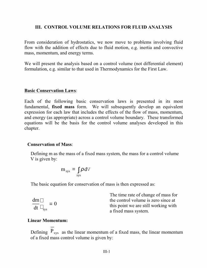
III-1

III. CONTROL VOLUME RELATIONS FOR FLUID ANALYSIS From consideration of hydrostatics, we now move to problems involving fluid flow with the addition of effects due to fluid motion, e.g. inertia and convective mass, momentum, and energy terms. We will present the analysis based on a control volume (not differential element) formulation, e.g. similar to that used in Thermodynamics for the First Law. Basic Conservation Laws:

Each of the following basic conservation laws is presented in its most fundamental, fixed mass form. We will subsequently develop an equivalent expression for each law that includes the effects of the flow of mass, momentum, and energy (as appropriate) across a control volume boundary. These transformed equations will be the basis for the control volume analyses developed in this chapter.

Conservation of Mass:

Defining m as the mass of a fixed mass system, the mass for a control volume V is given by:

m sys = ρdV

sys∫

The basic equation for conservation of mass is then expressed as:

dmdt

sys

= 0

The time rate of change of mass for the control volume is zero since at this point we are still working with a fixed mass system.

Linear Momentum:

Defining P sys as the linear momentum of a fixed mass, the linear momentum of a fixed mass control volume is given by:

III-2

III-3

P sys = mV = V ρdV

sys∫

where: V is the local fluid velocity and dV is a differential volume element in the control volume. The basic linear momentum equation is then written as:

F =∑ dP dt

sys=

d mV ( )dt

sys

Moment of Momentum: Defining H as the moment of momentum for a fixed mass, the moment of momentum for a fixed mass control volume is given by:

H sys = r × V ρdV

sys∫

where r is the moment arm from an inertial coordinate system to the differential control volume of interest. The basic equation is then written as:

M sys = r ×∑ F =∑ dH dt

sys

Energy: Defining Esys as the total energy of an element of fixed mass, the energy of a fixed mass control volume is given by:

Esys = eρ dV

sys∫

III-4

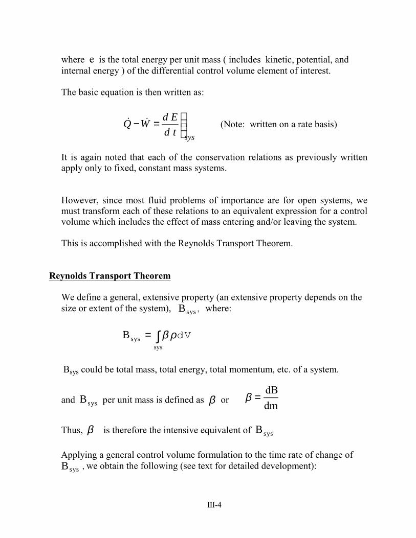
where e is the total energy per unit mass ( includes kinetic, potential, and internal energy ) of the differential control volume element of interest. The basic equation is then written as:

systdEdWQ

=− !! (Note: written on a rate basis)

It is again noted that each of the conservation relations as previously written apply only to fixed, constant mass systems. However, since most fluid problems of importance are for open systems, we must transform each of these relations to an equivalent expression for a control volume which includes the effect of mass entering and/or leaving the system. This is accomplished with the Reynolds Transport Theorem.

Reynolds Transport Theorem We define a general, extensive property (an extensive property depends on the size or extent of the system), Bsys , where:

Bsys = β ρdV

sys∫

Bsys could be total mass, total energy, total momentum, etc. of a system.

and Bsys per unit mass is defined as β or β =

dBdm

Thus, β is therefore the intensive equivalent of Bsys

Applying a general control volume formulation to the time rate of change of

Bsys , we obtain the following (see text for detailed development):

III-5

dBdt

sys

=∂∂t

β ρcv∫ dV + β e

Ae

∫ ρe Ve dAe − β iAi

∫ ρ i Vi dAi

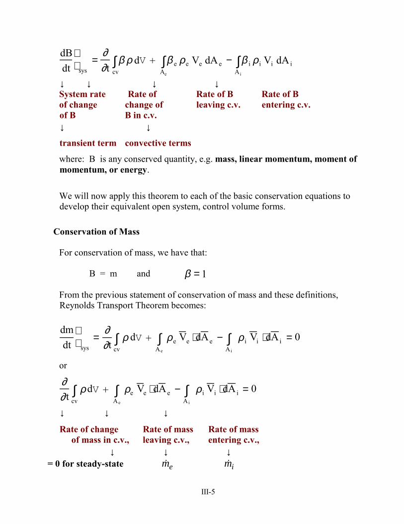
↓ ↓ ↓ ↓ System rate Rate of Rate of B Rate of B of change change of leaving c.v. entering c.v. of B B in c.v. ↓ ↓

transient term convective terms

where: B is any conserved quantity, e.g. mass, linear momentum, moment of momentum, or energy.

We will now apply this theorem to each of the basic conservation equations to develop their equivalent open system, control volume forms.

Conservation of Mass For conservation of mass, we have that:

B = m and β = 1 From the previous statement of conservation of mass and these definitions, Reynolds Transport Theorem becomes:

dmdt

sys

=∂∂t

ρcv∫ dV +

Ae

∫ ρe V e ⋅dA e −Ai

∫ ρ i V i ⋅dA i = 0

or

∂∂t

ρcv∫ dV +

Ae

∫ ρe V e ⋅ dA e −Ai

∫ ρ i V i ⋅dA i = 0

↓ ↓ ↓

Rate of change Rate of mass Rate of mass of mass in c.v., leaving c.v., entering c.v.,

↓ ↓ ↓ = 0 for steady-state em! im!

III-6

This can be simplified to

∑∑ =−+

0iecv

mmtdmd !!

Note that the exit and inlet velocities, Ve and Vi, are the local components of fluid velocities at the exit and inlet boundaries relative to an observer standing on the boundary. Therefore, if the boundary is moving, the velocity is measured relative to the boundary motion. The location and orientation of a coordinate system for the problem is not considered in determining these velocities. Also, the result of V e ⋅ dA e and V i ⋅dA i is the product of the normal velocity component times the flow area at the exit or inlet, e.g. Ve,n dAe and Vi,n dAi Special Case: For incompressible flow with a uniform velocity over the flow area, the previous integral expressions simplify to: ∫ == VAAdVm ρρ! Conservation of Mass Example

Water at a velocity of 7 m/s exits a stationary nozzle with D = 4 cm and is directed toward a turning vane with θ = 40û, assume steady-state. Determine: a. Velocity and flow rate entering the c.v. b. Velocity and flow rate leaving the c.v.

III-7

a. Find V1 and m!

Recall that the mass flow velocity is the normal component of velocity measured relative to the inlet or exit area. Thus, relative to the nozzle, V(nozzle) = 7 m/s and since there is no relative motion of point 1 relative to the nozzle, we also have V1 = 7 m/s ans. From the previous equation: ∫ == VAAdVm ρρ! = 998 kg/m3*7 m/s*π*.042/4 1m! = 8.78 kg/s ans.

b. Find V2 and 2m! Determine the flow rate first. Since the flow is steady state and no mass accumulates on the vane:

1m! = 2m! , 2m! = 8.78 kg/s ans. Now: 2m! = 8.78 kg/s = ρ A V)2 Since ρ and A are constant, V2 = 7 m/s ans. Key Point: For steady flow of a constant area, incompressible stream, the flow velocity and total mass flow are the same at the inlet and exit, even though the direction changes. or alternatively: Flexible Hose Concept: For steady flow of an incompressible fluid, the flow stream can be considered as an incompressible, flexible hose and if it enters a c.v. at a velocity of V, it exits at a velocity of V, even if it is redirected.

III-8

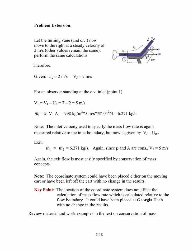
Problem Extension: Let the turning vane (and c.v.) now move to the right at a steady velocity of 2 m/s (other values remain the same), perform the same calculations.

Therefore: Given: Uc = 2 m/s VJ = 7 m/s

For an observer standing at the c.v. inlet (point 1) V1 = VJ � Uc = 7 � 2 = 5 m/s

1m! = ρ1 V1 A1 = 998 kg/m3*5 m/s*π*.042/4 = 6.271 kg/s Note: The inlet velocity used to specify the mass flow rate is again measured relative to the inlet boundary, but now is given by VJ � Uc . Exit: 1m! = 2m! = 6.271 kg/s, Again, since ρ and A are cons., V2 = 5 m/s Again, the exit flow is most easily specified by conservation of mass concepts. Note: The coordinate system could have been placed either on the moving cart or have been left off the cart with no change in the results. Key Point: The location of the coordinate system does not affect the

calculation of mass flow rate which is calculated relative to the flow boundary. It could have been placed at Georgia Tech with no change in the results.

Review material and work examples in the text on conservation of mass.

III-9

Linear Momentum For linear momentum, we have that:

B = P = mV and β = V From the previous statement of linear momentum and these definitions, Reynolds Transport Theorem becomes:

F =∑

d mV dt

sys=

∂∂t

V ρcv∫ dV + V

Ae

∫ ρe V e ⋅dA e − V Ai

∫ ρ i V i ⋅dA i

or

∫∫ ∫∑ −+∂∂=

ie Ai

cv Ae mdVmdVVdV

tF !!ρ

↓ ↓ ↓ ↓ = the ∑ of the = the rate of = the rate of = the rate of external forces change of momentum momentum acting on the c.v. momentum leaving the entering the c.v. in the c.v. c.v.

↓ ↓ = body + point + = 0 for distributed, e.g. steady-state (pressure) forces

and where V is the vector momentum velocity relative to an inertial reference frame.

Key Point: Thus, the momentum velocity has magnitude and direction and is measured relative to the reference frame (coordinate system) being used for the problem. The velocity in the mass flow terms, Ý m i and Ý m e ,is a scalar, as noted previously, and is measured relative to the inlet or exit boundary.

Always clearly define a coordinate system and use it to specify the value of all inlet and exit momentum velocities when working linear momentum problems.

III-10

For the 'x' direction, the previous equation becomes:

∫∫ ∫∑ −+∂∂=

ie Aiix

cv Aeexxx mdVmdVVdV

tF !! ,,ρ

Note that the above equation is also valid for control volumes moving at constant velocity with the coordinate system placed on the moving control volume. This is because an inertial coordinate system is a non - accelerating coordinate system which is still valid for a c.s. moving at constant velocity. Example: A water jet 4 cm in diameter with a velocity of 7 m/s is directed to a stationary turning vane with θ = 40û. Determine the force, F, necessary to hold the vane stationary.

Governing Equation:

∫∫ ∫∑ −+∂∂=

ie Aiix

cv Aeexxx mdVmdVVdV

tF !! ,,ρ

Since the flow is steady and the c.v. is stationary, the time rate of change of momentum within the c.v. is zero. Also, with uniform velocity at each inlet and exit and a constant flow rate, the momentum equation becomes:

iieeb VmVmF !! −=−

Note that the braking force, Fb, is written as negative since it is assumed to be in the negative �x� direction relative to positive �x� from the coordinate system.

III-11

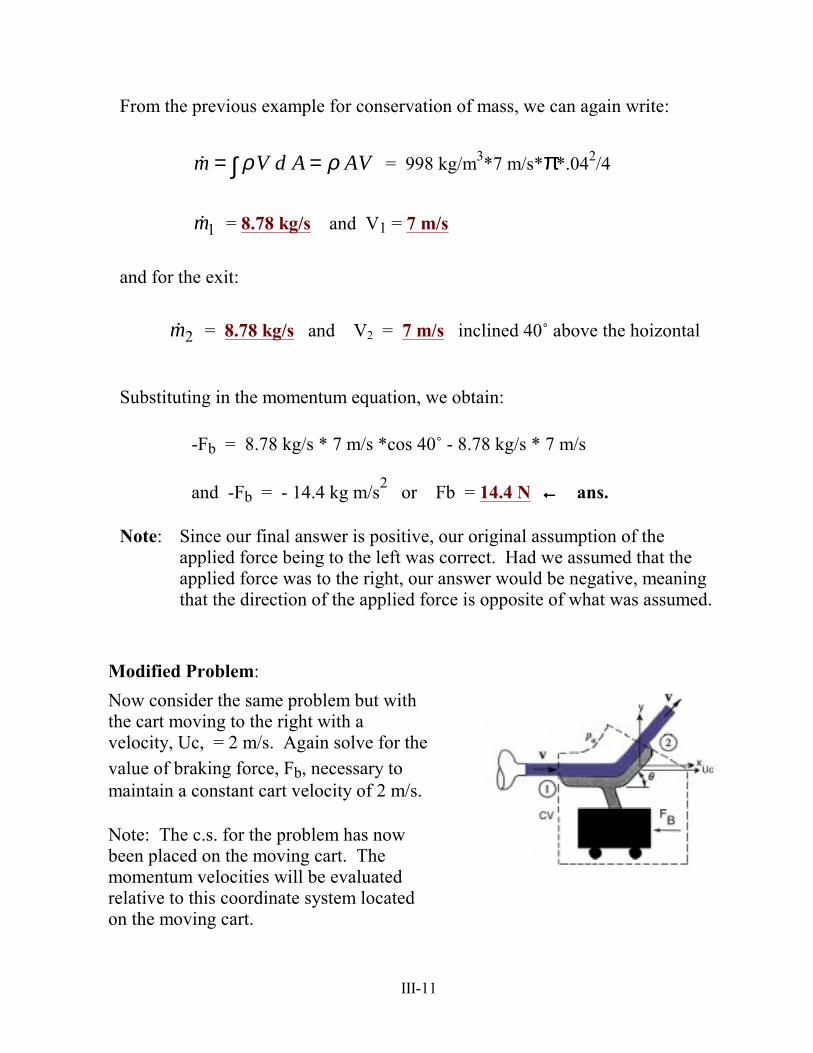
From the previous example for conservation of mass, we can again write: ∫ == VAAdVm ρρ! = 998 kg/m3*7 m/s*π*.042/4

1m! = 8.78 kg/s and V1 = 7 m/s

and for the exit: 2m! = 8.78 kg/s and V2 = 7 m/s inclined 40û above the hoizontal Substituting in the momentum equation, we obtain: -Fb = 8.78 kg/s * 7 m/s *cos 40û - 8.78 kg/s * 7 m/s and -Fb = - 14.4 kg m/s2 or Fb = 14.4 N ← ← ← ← ans. Note: Since our final answer is positive, our original assumption of the

applied force being to the left was correct. Had we assumed that the applied force was to the right, our answer would be negative, meaning that the direction of the applied force is opposite of what was assumed.

Modified Problem: Now consider the same problem but with the cart moving to the right with a velocity, Uc, = 2 m/s. Again solve for the value of braking force, Fb, necessary to maintain a constant cart velocity of 2 m/s.

Note: The c.s. for the problem has now been placed on the moving cart. The momentum velocities will be evaluated relative to this coordinate system located on the moving cart.

III-12

The transient term in the momentum equation is still zero. With the coordinate system on the cart, the momentum of the cart relative to the coordinate system is still zero. The fluid stream is still moving relative to the coordinate system, however, the flow is steady with constant velocity and the time rate of change of momentum of the fluid stream is therefore also zero. Thus: The momentum equation has the same form as for the previous problem (however, the value of individual terms will be different). iieeb VmVmF !! −=−

1m! = ρ1 V1 A1 = 998 kg/m3*5 m/s*π*.042/4 = 6.271 kg/s = 2m! Now determine the momentum velocity at the inlet and exit. With the c.s. on the moving c.v., the values of momentum velocity are

V1 = VJ � Uc = 7 � 2 = 5 m/s and V2 = 5 m/s inclined 40û . The momentum equation ( �x� direction ) now becomes:

-Fb = 6.271 kg/s * 5 m/s *cos 40û - 6.271 kg/s * 5 m/s

and -Fb = - 7.34 kg m/s2 or Fb = 7.34 N ← ← ← ← ans. Question: What would happen to the braking force, Fb, if the turning angle had been > 90û, e.g. 130û? Can you explain based on your understanding of change in momentum for the fluid stream? Review and work examples for linear momentum with fixed and non - accelerating (moving at constant velocity) control volumes.

Accelerating Control Volume The previous formulation applies only to inertial coordinate systems, i.e. fixed or moving at constant velocity (non-accelerating).

III-13

We will now consider problems with accelerating control volumes. For these problems we will again place the coordinate system on the accelerating control volume thus making it a non-inertial coordinate system. For coordinate systems placed on an accelerating control volume, we must account for the acceleration of the c.s. by correcting the momentum equation for this acceleration. This is accomplished by including the term as shown below:

∫∫ ∫∑ ∫ −+∂∂=−

ie Ai

cv Aecv

cvcv mdVmdVVdV

tmdaF !!ρ

↓

integral sum of the local c.v. (c.s.) accel. * the c.v. mass The added term accounts for the acceleration of the control volume and allows the problem to be worked with the coordinate system placed on the accelerating c.v. Note: Thus, all vector (momentum) velocities are then measured relative to an observer (coordinate system) on the accelerating control volume. For example, the velocity of a rocket as seen by an observer (c.s.) standing on the rocket is zero and the time rate of change of momentum is zero in this reference frame even if the rocket is accelerating. Accelerating Control Volume Example

A turning vane with θ = 60û accelerates from rest due to a jet of water (VJ = 35 m/s, AJ = .003 m2 ). Assuming the mass of the cart, mc, is 75 kg and neglecting drag and friction effects, find: a. Cart acceleration at t = 0.

III-14

b. Uc f(t)

III-15

Starting with the general equation shown above, we can make the following assumptions:

1. ∑ Fx = 0, no friction or body forces. 2. The jet has uniform velocity and constant properties. 3. The entire cart accelerates uniformly over the entire control volume. 4. Neglect the relative momentum change of the jet stream that is within the

control volume. With these assumptions, the governing equation simplifies to:

-ac mc = Ý m e Ux,e - Ý m i Ux,i We thus have terms that account for the acceleration of the control volume, for the exit momentum, and for the inlet momentum (both of which change with time). mass flow: As with the previous example for a moving control volume, the mass flow terms are given by:

=== mmm ei !!! ρ AJ (VJ � Uc)

Note that since the cart accelerates, Uc is not a constant, but rather changes with time. momentum velocities:

Ux,i= VJ - Uc Ux,e = (VJ - Uc ) cos θ

Substituting, we now obtain:

- ac mc = ρ AJ (VJ � Uc)2 cos θ - ρ AJ (VJ � Uc) Solving for the cart acceleration, we obtain:

ac =ρ AJ 1 − cosθ( ) VJ − Uc( )2

mc

III-16

Substituting for the given values at t = 0, i.e. Uc = 0, we obtain:

ac (t = 0) = 24.45 m/s2 = 2.49 g�s Note: The acceleration at any other time can be obtained once the cart

velocity, Uc, at that time is known. To determine the equation for cart velocity as a function of time, the equation for the acceleration must be written in terms of Uc(t) and integrated.

dUcdt =

ρ AJ 1 −cosθ( )VJ −Uc( )2mc

Separating variables, we obtain:

dUc

VJ − Uc( )20

Uc (t )

∫ =ρ AJ 1 − cosθ( )

mc0

t

∫ dt

Completing the integration and rearranging the terms, we obtain a final expression of the form:

Uc

VJ

=VJ b t

1+ VJ b t where b =ρ AJ 1 − cosθ( )

mc

Substituting for known values, we obtain: VJ b = .699 s-1 Thus, the final equation for Uc is give by:

Uc

VJ=

0.699 t1+0.699 t

III-17

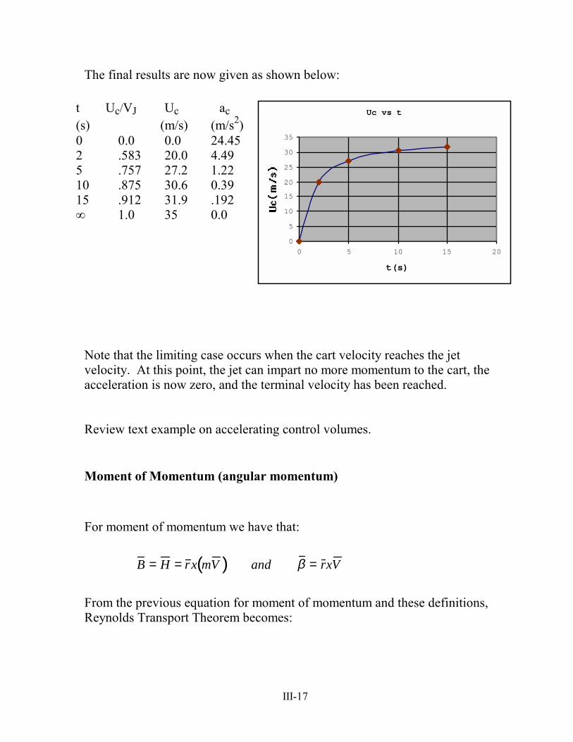
The final results are now given as shown below:

t Uc/VJ Uc ac (s) (m/s) (m/s2) 0 0.0 0.0 24.45 2 .583 20.0 4.49 5 .757 27.2 1.22 10 .875 30.6 0.39 15 .912 31.9 .192 ∞ 1.0 35 0.0

Uc vs t

0

5

10

15

20

25

30

35

0 5 10 15 20

t(s)

Note that the limiting case occurs when the cart velocity reaches the jet velocity. At this point, the jet can impart no more momentum to the cart, the acceleration is now zero, and the terminal velocity has been reached. Review text example on accelerating control volumes. Moment of Momentum (angular momentum) For moment of momentum we have that:

B = H = r x mV ( ) and β = r xV From the previous equation for moment of momentum and these definitions, Reynolds Transport Theorem becomes:

III-18

∫∫ ∫∑ −+∂∂=

ie Ai

cv Ae mdVxrmdVxrVdVxr

tM !!ρ

↓ ↓ ↓ ↓ = the ∑ of all = the rate of = the rate of = the rate of external change of mom- moment of moment of moments ent of momentum momentum momentum acting in the c.v. = 0 leaving entering on the c.v. for steady state the c.v. the c.v. For the special case of steady-state, steady-flow and uniform properties at any exit or inlet, the equation becomes:

∑∑∑ −= iiee VxrmVxrmM !! For moment of momentum problems, we must be careful to correctly evaluate the moment of all applied forces and all inlet and exit momentum flows, with particular attention to the signs. Moment of Momentum Example: A small lawn sprinkler operates as indicated. The inlet flow rate is 9.98 kg/min with an inlet pressure of 30 kPa. The two exit jets direct flow at an angle of 40û above the horizontal. For these conditions, determine the following: a. jet velocity relative to the nozzle b. torque require to hold the arm stationary c. friction torque if the arm is rotating at 35 rpm d. maximum rotational speed if we neglect friction.

160 mm

D = 5 mmJ

III-19

R = 160 mm, DJ = 5 mm, Therefore, for each of the two jets:

QJ = 0.5* 9.98 kg/min/998 kg/m3 = .005 m3/min

AJ = π .00252 = 1.963*10-5 m2

VJ = .005 m3/min / 1.963*10-5 m2 /60 sec/min VJ = 4.24 m/s relative to the nozzle exit ans.

b. torque required to hold the arm stationary First develop the governing equations and analysis for the general case of the arm rotating.

With the coordinate system at the center of rotation of the arm, a general velocity diagram for the case when the arm is rotating is shown in the adjacent schematic.

R

V cos θJ

oω

rω

+

Taking the moment about the center of rotation, the moment of the inlet flow is zero since the moment arm is zero for the inlet flow.

The basic equation then becomes:

{ }ωα RVRmT Jeo −= cos2 ! Note that the net momentum velocity is the difference between the tangential component of the jet exit velocity and the rotational speed of the arm. Also note that the direction of positive moments was taken as the same as for VJ and opposite of the direction of rotation.

For a stationary arm: R ω = 0. We thus obtain for the stationary torque:

III-20

To = 2 ρ QJ R VJ cos α

To = 2 * 998 kgm3 .005 m3

min1min60sec

.16m * 4.24 ms

cos 40o

To = 0.0864 N m clockwise. ans.

A resisting torque of .0864 Nm must be applied in the clockwise direction to keep the arm from rotating in the counterclockwise direction. c. At ω = 30 rpm, calculate the friction torque, Tf

ω = 30 revmin

2π radrev

1min60sec

=π radsec

To = 2 * 998 kg

m3 .005 m3

min1min60sec

.16m 4.24 ms

cos 40o − .16m * πradsec

To = .0685 Nm ans.

Note: The resisting torque decreases as the speed increases. d. Find the maximum rotational speed. The maximum rotational speed occurs when the opposing torque is zero and all the moment of momentum goes to the angular rotation. For this case,

VJ cos θ � Rω = 0

ω =VJ cosθ

R= 4.24m / s •cos 40

.16 m= 20.3 rad

sec=193.8 rpm ans.

Review material and examples on moment of momentum.

III-21

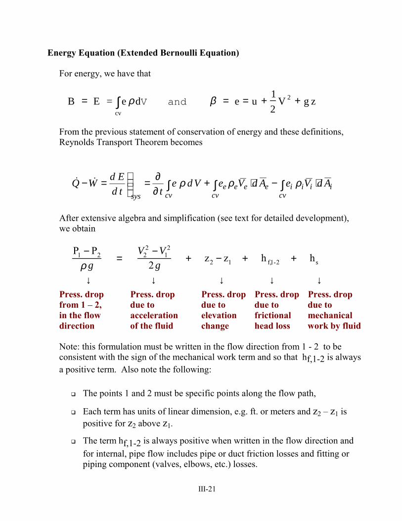
Energy Equation (Extended Bernoulli Equation) For energy, we have that

B = E = eρdcv∫ V and β = e = u + 1

2V 2 + g z

From the previous statement of conservation of energy and these definitions, Reynolds Transport Theorem becomes

iiicv

ieeecv cv

esys

AdVeAdVeVdettd

EdWQ ⋅−⋅+∂∂=

=− ∫∫ ∫ ρρρ!!

After extensive algebra and simplification (see text for detailed development), we obtain

P1 − P2

ρ g =V2

2 −V12

2 g + z2 − z1 + h f,1-2 + hs

↓ ↓ ↓ ↓ ↓ Press. drop Press. drop Press. drop Press. drop Press. drop from 1 � 2, due to due to due to due to in the flow acceleration elevation frictional mechanical direction of the fluid change head loss work by fluid Note: this formulation must be written in the flow direction from 1 - 2 to be consistent with the sign of the mechanical work term and so that hf,1-2 is always a positive term. Also note the following:

! The points 1 and 2 must be specific points along the flow path,

! Each term has units of linear dimension, e.g. ft. or meters and z2 � z1 is positive for z2 above z1.

! The term hf,1-2 is always positive when written in the flow direction and for internal, pipe flow includes pipe or duct friction losses and fitting or piping component (valves, elbows, etc.) losses.

III-22

! The term hs is negative for pumps and fans, - hp ( i.e. pumps increase the

pressure in the flow direction) and positive for turbines, + ht (turbines decrease the pressure in the flow direction).

! For pumps:

h p = ws

g Where: ws = the useful work per unit mass to the fluid

Therefore: ws = g hp and == sf wmW !! ρ Q g hp

Where: fW! = the useful power delivered to the fluid

and: pp

fp and

WW η

η

!! = is the pump efficiency

Water flows at 30 ft/s through a 1000 ft length of 2 in. diameter pipe. The inlet pressure is 250 psig and the exit is 100 ft higher than the inlet. Assuming that the frictional loss is given by 18 V2/2g: Determine the exit pressure.

1

2

100 ft

250 psig

2

Given: V1 = V2 = 30 ft/s, L = 1000 ft, Z2 � Z1 = 100 ft, P1 = 250 psig Also, since there is no mechanical work in the process, the energy equation simplifies to:

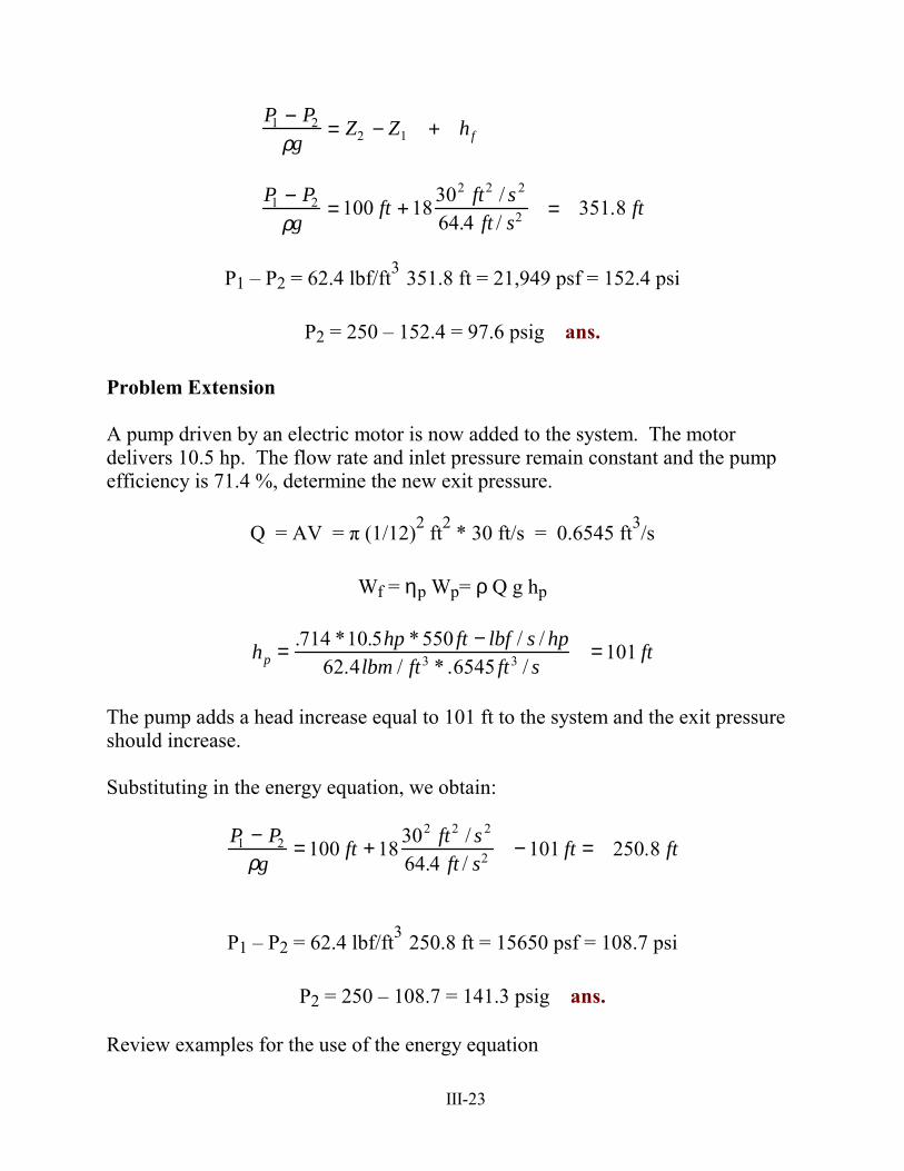
III-23

P1 − P2

ρg= Z2 − Z1 + hf

P1 − P2

ρg= 100 ft +18 302 ft2 / s 2

64.4 ft / s2 = 351.8 ft

P1 � P2 = 62.4 lbf/ft3 351.8 ft = 21,949 psf = 152.4 psi

P2 = 250 � 152.4 = 97.6 psig ans.

Problem Extension A pump driven by an electric motor is now added to the system. The motor delivers 10.5 hp. The flow rate and inlet pressure remain constant and the pump efficiency is 71.4 %, determine the new exit pressure.

Q = AV = π (1/12)2 ft2 * 30 ft/s = 0.6545 ft3/s

Wf = ηp Wp= ρ Q g hp

hp = .714 *10.5hp * 550 ft − lbf / s / hp62.4lbm / ft3 * .6545 ft3 / s

=101 ft

The pump adds a head increase equal to 101 ft to the system and the exit pressure should increase. Substituting in the energy equation, we obtain:

P1 − P2

ρg= 100 ft +18 302 ft2 / s 2

64.4 ft / s2 −101 ft = 250.8 ft

P1 � P2 = 62.4 lbf/ft3 250.8 ft = 15650 psf = 108.7 psi

P2 = 250 � 108.7 = 141.3 psig ans.

Review examples for the use of the energy equation

III-24

Kinetic Energy Correction Factor Up to this point, the velocity used in the kinetic energy term of the energy equation has been the mass average velocity obtained from the definition of flow rate,

VAm ρ=!

However, since V varies over the flow area and the kinetic energy term varies with the square of the velocity, using this definition of V may not result in an accurate evaluation of the kinetic energy term for the flow. This problem can be corrected through the use of the kinetic energy correction factor , α , defined for incompressible flow from

12

ρ u3d A =12∫ ρα Vav

3 A

Solving for α we obtain α =1A

uVav

3

∫ d A

For fully developed laminar flow, α = 2 and for turbulent pipe flow, a value from 1.04 to 1.11. Using the kinetic energy correction factor, the energy equation becomes

P1 − P2

ρ g =αV2

2 −αV12

2g + z2 − z1 + h f,1-2 + hs

While subsequent analyses and examples in these notes will continue to use the energy equation omitting the kinetic energy correction factor (α = 1), students are reminded to used this term where appropriate for pipe flow analyses.

III-25

The Bernoulli Equation The Bernoulli equation is an equation that is closely related to the energy equation and is useful in the analysis of many flows. The most common application is for steady, incompressible, frictionless flow between two points along a stream line. For these conditions, Bernoulli�s equation becomes

P1ρ

+V1

2

2+ g z1 =

P2ρ

+V2

2

2+ g z2 = const

where the constant is the same along a specified streamline. Different streamlines may have different Bernoulli constants. Bernoulli�s equation can also be written as

P2 − P1ρ

+V2

2 − V12

2+ g z2 − z1( )= 0

Students must be careful not to misuse Bernoulli�s equation. In particular, do not use the Bernoulli equation for flows with any or all of the following:

1. friction between points 1 and 2 2. shaft work between points 1 and 2 3. heat transfer between points 1 and 2 4. significant compressibility effects between 1 and 2

Hydraulic and Energy Grade Lines

Hydraulic and energy grade lines are lines that provide a very helpful visual representation of what is happening to key flow and energy equation parameters between points in the flow. They are defined as follows:

energy grade line (EGL) - a line that shows the variation of the height of the total Bernoulli constant,

ho =P

ρ g+

V22 g

+ z

III-26

The EGL has a constant height for steady, frictionless, incompressible flow with no heat transfer or shaft work.

III-27

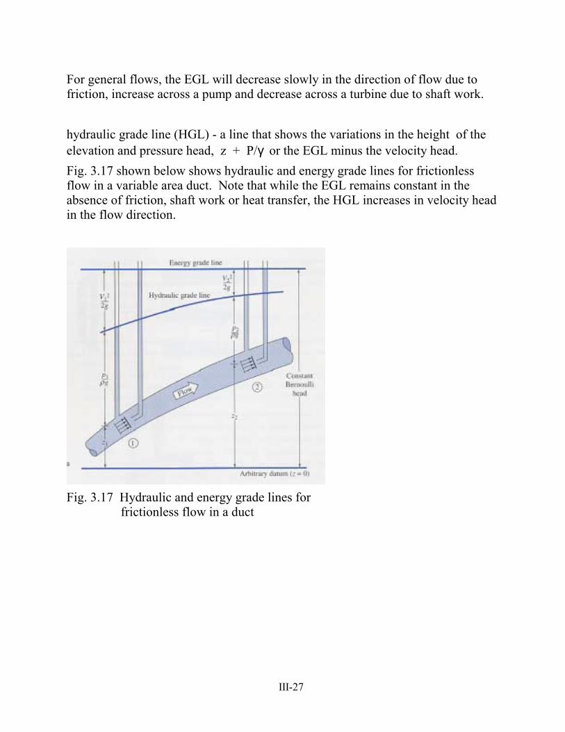
For general flows, the EGL will decrease slowly in the direction of flow due to friction, increase across a pump and decrease across a turbine due to shaft work. hydraulic grade line (HGL) - a line that shows the variations in the height of the elevation and pressure head, z + P/γ or the EGL minus the velocity head. Fig. 3.17 shown below shows hydraulic and energy grade lines for frictionless flow in a variable area duct. Note that while the EGL remains constant in the absence of friction, shaft work or heat transfer, the HGL increases in velocity head in the flow direction.

Fig. 3.17 Hydraulic and energy grade lines for frictionless flow in a duct