III Concepts in Probability, Statistics and Stochastic Modeling 1. Introduction

2. Probability concepts and methods

2.1 Random variables and distributions 2.2 Expectation operator 2.3 Quantiles, moments, and their estimators 2.4 L-Moments and their estimators

3. Distributions of random events

3.1 Parameter estimation 3.2 Model adequacy 3.3 Normal and lognormal distributions 3.4 Gamma distributions 3.5 Log-Pearson type 3 distribution 3.6 Gumbel and GEV distributions 3.7 L-moment diagrams

4. Analysis of censored data

5. Regionalization and index-flood method

6. Partial duration series

7. Stochastic processes and time series 7.1 Describing stochastic processes 7.2 Markov processes and Markov chains 7.3 Properties of time-series statistics

8. Synthetic streamflow generation 8.1 Introduction 8.2 Streamflow generation models 8.3 A simple autoregressive model 8.4 Reproducing the marginal distribution 8.5 Multivariate models 8.6 Multi-season, multi-site models

9. Stochastic simulation

9.1 Generating random variables 9.2 River basin simulation. 9.3 The simulation model 9.4 Simulation of the basin 9.5 Interpreting simulation output

10. Conclusions

11. References

Events that cannot be predicted precisely are often called random. Many if not most of the

inputs to, and processes that occur in, water resource systems are to some extent random.

Hence so too are the outputs or predicted impacts, and even people’s reactions to those

outputs or impacts. Ignoring this randomness or uncertainty when performing analyses in

support of decisions involving the development and management of water resource systems

is to ignore reality. This chapter introduces some of the commonly used tools for dealing

with uncertainty in water resources planning and management. Subsequent chapters

illustrate how many of these tools are used in various types of optimization, simulation and

statistical models for impact prediction and evaluation.

1. Introduction Uncertainty is always present when planning, developing, managing and operating water

resource systems. It arises because many factors that affect the performance of water resource

systems are not and cannot be known with certainty when a system is planned, designed, built,

managed and operated. The success and performance of each component of a system often

depends on future meteorological, demographic, economic, social, technical, and political

conditions, all of which may influence future benefits, costs, environmental impacts, and social

acceptability. Uncertainty also arises due to the stochastic nature of meteorological processes

such as evaporation, rainfall, and temperature. Similarly, future populations of towns and cities,

per capita water usage rates, irrigation patterns, and priorities for water uses, all of which impact

water demand, are never known with certainty.

This chapter introduces methods for describing and dealing with uncertainty, and provides some

simple examples of their use in water resources planning.

There are many ways to deal with uncertainty. One, and perhaps the simplest, approach is to

replace each uncertain quantity either by its average (i.e., its mean or expected value), its median,

or by some critical (e.g., “worst-case”) value and then proceed with a deterministic approach.

Use of expected or median values of uncertain quantities may be adequate if the uncertainty or

variation in a quantity is reasonably small and does not critically affect the performance of the

system. If expected or median values of uncertain parameters or variables are used in a

deterministic model, the planner can then assess the importance of uncertainty using sensitivity

analysis, as is discussed later in this and subsequent chapters.

Replacement of uncertain quantities by either expected, median or worst-case values can grossly

affect the evaluation of project performance when important parameters are highly variable. To

illustrate these issues, consider the evaluation of the recreation potential of a reservoir. Table 3.1

shows that the elevation of the water surface varies from year to year depending on the inflow

and demand for water. The table indicates the pool levels and their associated probabilities as

well as the expected use of the recreation facility with different pool levels.

Table 3.1 Data for Determining Reservoir Recreation Potential.

The average pool level L is simply the sum of each possible pool level times its probability, or L = 10(0.10) + 20(0.25) + 30(0.30) + 40(0.25) +50(0.10) = 30 (3.1)

This pool level corresponds to 100 visitor-days per day:

VD ( )L = 100 visitor-days per day (3.2)

A worst-case analysis might select a pool level of 10 as a critical value, yielding an estimate of

system performance equal to 25 visitor-days per day:

VD(Llow) = VD(10) = 25 visitor-days per day (3.3)

Neither of these values is a good approximation of the average visitation rate, that is

VD = 0.10 VD(10) + 0.25 VD(20) + 0.30 VD(30) + 0.25 VD(40) + 0.10 VD(50)

= 0.10(25) + 0.25(75) + 0.30(100) + 0.25(80) + 0.10(70) (3.4)

= 78.25 visitor-days per day

Clearly, the average visitation rate, VD = 78.25, the visitation rate corresponding to the average

pool level VD(L) = 100, and the worst-case assessment VD(Llow) = 25, are very different.

Using only average values in a complex model can produce a poor representation of both the

average performance and the possible performance range. When important quantities are

uncertain, a comprehensive analysis requires an evaluation of both the expected performance of a

project and the risk and possible magnitude of project failures in a physical, economic,

ecological, and/or social sense.

This chapter reviews many of the methods of probability and statistics that are useful in water

resources planning and management. Section 2 is a condensed summary of the important

concepts and methods of probability and statistics. These concepts are applied in this and

subsequent chapters of this book. Section 3 presents several probability distributions that are

often used to model or describe the distribution of uncertain quantities. The section also

discusses methods for fitting these distributions using historical information, and methods of

assessing whether the distributions are adequate representations of the data. Sections 4, 5 and 6

expand upon the use of these mathematical models, and discuss alternative parameter estimation

methods.

Section 7 presents the basic ideas and concepts of the stochastic processes or time series. These

are used to model streamflows, rainfall, temperature, or other phenomena whose values change

with time. The section contains a description of Markov chains, a special type of stochastic

process used in many stochastic optimization and simulation models. Section 8 illustrates how

synthetic flows and other time series inputs can be generated for stochastic simulations.

Stochastic simulation is introduced with an example in Section 9.

Many topics receive only brief treatment in this introductory chapter. Additional information

can be found in applied statistical texts or book chapters such as Benjamin and Cornell (1970),

Haan (1977), Kite (1988), Stedinger et al. (1993), Kottegoda and Rosso (1997), and Ayyub and

McCuen, (2002).

2. Probability concepts and methods

This section introduces the basic concepts and definitions used in analyses involving probability

and statistics. These concepts are used throughout this chapter and later chapters in the book.

2.1 Random variables and distributions

The basic concept in probability theory is that of the random variable. By definition, the value

of a random variable cannot be predicted with certainty. It depends, at least in part, on the

outcome of a chance event. Examples are (1) the number of years until the flood stage of a river

washes away a small bridge, (2) the number of times during a reservoir’s life that the level of the

pool will drop below a specified level, (3) the rainfall depth next month, and (4) next year’s

maximum flow at a gage site on an unregulated stream. The values of all of these random events

or variables are not knowable before the event has occurred. Probability can be used to describe

the likelihood that these random variables will equal specific values or be within a given range of

specific values.

The first two examples illustrate discrete random variables, random variables that take on values

that are discrete (such as positive integers). The second two examples illustrate continuous

random variables. Continuous random variables take on any values within a specified range of

values. A property of all continuous random variables is that the probability that the value of

any of those random variables will equal some specific number – any specific number – is

always zero. For example, the probability that the total rainfall depth in a month will be exactly

5.0 cm is zero, while the probability that the total rainfall will lie between 4 and 6 cm can be

nonzero. Some random variables are combinations of continuous and discrete random variables.

Let X denote a random variable and x a possible value of that random variable X. Random

variables are generally denoted by capital letters and particular values they take on by lowercase

letters. For any real-valued random variable X, its cumulative distribution function FX(x), often

denoted as just the cdf, equals the probability that the value of X is less than or equal to a specific

value or threshold x:

FX(x) = Pr[X ≤ x] (3.5)

This cumulative distribution function FX(x) is a non-decreasing function of x because

Pr[X ≤ x] ≤ Pr[X ≤ x + δ] for δ > 0 (3.6)

In addition,

(3.7) lim ( ) 1XxF x

→+∞=

and

(3.8) lim ( ) 0XxF x

→−∞=

The first limit equals 1 because the probability that X takes on some value less than infinity must

be unity; the second limit is zero because the probability that X takes on no value must be zero.

The left half of Figure 3.1 illustrates the cumulative distribution function (upper) and its

derivative, the probability density function, fX(x), (lower) of a continuous random variable X.

If X is a real-valued discrete random variable that takes on specific values x1, x2, . . . , the

probability mass function pX(xi) is the probability X takes on the value xi.

pX(xi) = Pr[X = xi] (3.9)

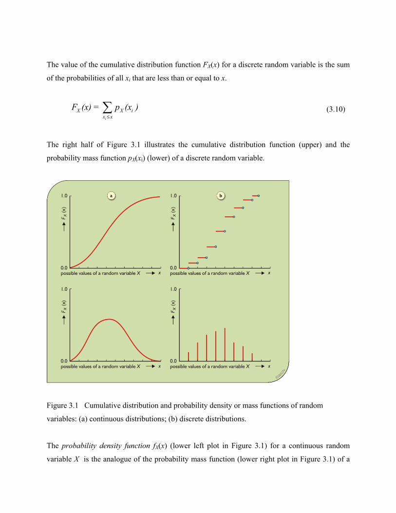
The value of the cumulative distribution function FX(x) for a discrete random variable is the sum

of the probabilities of all xi that are less than or equal to x.

i

X Xx x

F (x) = p (x )≤

∑ i (3.10)

The right half of Figure 3.1 illustrates the cumulative distribution function (upper) and the

probability mass function pX(xi) (lower) of a discrete random variable.

Figure 3.1 Cumulative distribution and probability density or mass functions of random

variables: (a) continuous distributions; (b) discrete distributions.

The probability density function fX(x) (lower left plot in Figure 3.1) for a continuous random

variable X is the analogue of the probability mass function (lower right plot in Figure 3.1) of a

discrete random variable X. The probability density function, often called the pdf, is the

derivative of the cumulative distribution function so that

( )( ) 0XX

dF xf xdx

= ≥ (3.11)

It is necessary to have

(3.12) ( ) 1Xf x+∞

−∞=∫

Equation 3.12 indicates that the area under the probability density function is 1. If a and b are

any two constants, the cumulative distribution function or the density function may be used to

determine the probability that X is greater than a and less than or equal to b where

[ ]Pr ( ) ( ) ( )b

X X Xa

a X b F b F a f x dx< ≤ = − = ∫ (3.13)

The area under a probability density function specifies the relative frequency with which the

value of a continuous random variable falls within any specified range of values, i.e., interval

along the horizontal axis.

Life is seldom so simple that only a single quantity is uncertain. Thus, the joint probability

distribution of two or more random variables can also be defined. If X and Y are two continuous

real-valued random variables, their joint cumulative distribution function is

FXY(x, y) = Pr[X ≤ x and Y ≤ y] ( , )yx

XYf u v du dv−∞ −∞

= ∫ ∫ (3.14)

If two random variables are discrete, then

( , ) ( , )i i

XY XY i ix x y y

F x y P x y≤ ≤

= ∑ ∑ (3.15)

where the joint probability mass function is

PXY(xi, yi) = Pr[X = xi, and Y = yi] (3.16)

If X and Y are two random variables, and the distribution of X is not influenced by the value

taken by Y, and vice versa, the two random variables are said to be independent. For two

independent random variables X and Y, the joint probability that the random variable X will be

between values a and b and that the random variable Y will be between values c and d is simply

the product of those separate probabilities.

Pr[a ≤ X ≤ b and c ≤ Y ≤ d] = Pr[a ≤ X ≤ b] Pr[c ≤ Y ≤ d] (3.17)

This applies for any values a, b, c, and d. As a result,

FXY(x, y) = FX(x)FY(y) (3.18)

which implies for continuous random variables that

fXY(x, y) = fX(x)fY(y) (3.19)

and for discrete random variables that

pXY(x, y) = pX(x)pY(y) (3.20)

Other useful concepts are those of the marginal and conditional distributions. If X and Y are two

random variables whose joint cumulative distribution function FXY(x, y) has been specified, then

FX(x), the marginal cumulative distribution of X, is just the cumulative distribution of X ignoring

Y. The marginal cumulative distribution function of X equals

FX(x) = Pr[X ≤ x] = (3.21) lim ( , )XYyF x y

→∞

where the limit is equivalent to letting Y take on any value. If X and Y are continuous random

variables, the marginal density of X can be computed from

( ) ( , )X XYf x f x y+∞

−∞

= ∫ dy (3.22)

The conditional cumulative distribution function is the cumulative distribution function for X

given that Y has taken a particular value y. Thus the value of Y may have been observed and one

is interested in the resulting conditional distribution for the so far unobserved value of X. The

conditional cumulative distribution function for continuous random variables is given by

|

( , )( | ) Pr[ | ]

( )−∞= ≤ = =∫x

xy

X Yy

f s y dsF x y X x Y y

f y (3.23)

It follows that the conditional density function is

|( , )( | )( )

XYX Y

Y

f x yf x yf y

= (3.24)

For discrete random variables, the probability of observing X = x, given that Y = y equals

pX | Y (x | y) =pxy (x, y)

py(y) (3.25)

These results can be extended to more than two random variables. Kottegoda and Rosso (1997)

provide more detail.

2.2 Expectation operator

Knowledge of the probability density function of a continuous random variable, or of the

probability mass function of a discrete random variable, allows one to calculate the expected

value of any function of the random variable. Such an expectation may represent the average

rainfall depth, average temperature, average demand shortfall, or expected economic benefits

from system operation. If g is a real-valued function of a continuous random variable X, the

expected value of g(X) is

[ ( )] ( ) ( )XE g X g x f x dx+∞

−∞

= ∫ (3.26)

whereas for a discrete random variable

E [g( X )] = g( x i ) pX ( xi )xi∑ (3.27)

The expectation operator, E[ ⋅ ], has several important properties. In particular, the expectation

of a linear function of X is a linear function of the expectation of X. Thus if a and b are two

nonrandom constants,

E[a + bX] = a + bE[X] (3.28)

The expectation of a function of two random variables is given by

[ ( , )] ( , ) ( , )XYE g X Y g x y f x y dx dy+∞ +∞

−∞ −∞

= ∫ ∫

or

[ ( , )] ( , ) ( , )i i XY i ii j

E g X Y g x y p x y= ∑∑ (3.29)

If X and Y are independent, the expectation of the product of a function g(⋅) of X and a function

h(⋅) of Y is the product of the expectations

E[ g(X) h(Y) ] = E[g(X)] E[h(Y)] (3.30)

This follows from substitution of Equations 3.19 and 3.20 into Equation 3.29.

2.3 Quantiles, moments, and their estimators

While the cumulative distribution function provides a complete specification of the properties of

a random variable, it is useful to use simpler and more easily understood measures of the central

tendency and range of values that a random variable may assume. Perhaps the simplest approach

to describing the distribution of a random variable is to report the value of several quantiles. The

pth quantile of a random variable X is the smallest value xp such that X has a probability p of

assuming a value equal to or less than xp:

Pr[X < xp] ≤ p ≤ Pr[X ≤ xp] (3.31)

Equation 3.31 is written to insist if at some value xp, the cumulative probability function jumps

from less than p to more than p, then that value xp will be defined as the pth quantile even though

FX(xp) ≠ p. If X is a continuous random variable, then in the region where fX(x) > 0, the quantiles

are uniquely defined and are obtained by solution of

FX(xp) = p (3.32)

Frequently reported quantiles are the median x0.50 and the lower and upper quartiles x0.25 and

x0.75. The median describes the location or central tendency of the distribution of X because the

random variable is, in the continuous case, equally likely to be above as below that value. The

interquartile range [x0.25, x0.75] provides an easily understood description of the range of values

that the random variable might assume. The pth quantile is also the 100 p percentile.

In a given application, particularly when safety is of concern, it may be appropriate to use other

quantiles. In floodplain management and the design of flood control structures, the 100-year

flood x0.99 is a commonly selected design value. In water quality management, a river’s

minimum 7-day-average low flow expected once in 10 years is commonly used in the US as the

critical planning value: Here the one-in-ten year value is the 10 percentile of the distribution of

the annual minima of the 7-day average flows.

The natural sample estimate of the median x0.50 is the median of the sample. In a sample of size

n where x(1) ≤ x(2) ≤ . . . ≤ x(n) are the observed observations ordered by magnitude, and for a non-

negative integer k such that n = 2k (even) or n = 2k + 1 (odd), the sample estimate of the median

is

( 1)

0.50( ) ( +1)

for = 2 + 1ˆ 1 + for = 2

2

+⎧⎪= ⎨

⎡ ⎤⎪ ⎣ ⎦⎩

k

k k

x nx

k

x x n k (3.33)

Sample estimates of other quantiles may be obtained by using x(i) as an estimate of xq for q = i/(n

+ 1) and then interpolating between observations to obtain ˆ px for the desired p. This only works

for 1/(n + 1) ≤ p ≤ n/(n + 1) and can yield rather poor estimates of xp when (n + 1)p is near either

1 or n. An alternative approach is to fit a reasonable distribution function to the observations, as

discussed in Section 3.1-3.2, and then estimate xp using Equation 3.32, where FX(x) is the fitted

distribution.

Another simple and common approach to describing a distribution’s center, spread, and shape is

by reporting the moments of a distribution. The first moment about the origin µX is the mean of

X and is given by

[ ] ( )X E X x f x dx+∞

−∞

= = ∫µ X (3.34)

Moments other than the first are normally measured about the mean. The second moment

measured about the mean is the variance, denoted Var(X) or 2Xσ , where:

(3.35) 2 Var( ) [ ( ) ]= = −X X E Xσ 2Xµ

The standard deviation σX is the square root of the variance. While the mean µX is a measure of

the central value of X, the standard deviation σX is a measure of the spread of the distribution of

X about µX.

Another measure of the variability in X is the coefficient of variation,

XX

X

CV σµ

= (3.36)

The coefficient of variation expresses the standard deviation as a proportion of the mean. It is

useful for comparing the relative variability of the flow in rivers of different sizes, or of rainfall

variability in different regions. Both are strictly positive values.

The third moment about the mean, denoted λX, measures the asymmetry or skewness of the

distribution:

λX = E[(X - µX)3] (3.37)

Typically, the dimensionless coefficient of skewness γX is reported rather than the third moment

λX. The coefficient of skewness is the third moment rescaled by the cube of the standard

deviation so as to be dimensionless and hence unaffected by the scale of the random variable:

3X

XX

λγσ

= (3.38)

Streamflows and other natural phenomena that are necessarily non-negative often have

distributions with positive skew coefficients, reflecting the asymmetric shape of their

distributions.

When the distribution of a random variable is not known, but a set of observations {x1, . . . , xn}

is available, the moments of the unknown distribution of X can be estimated based on the sample

values using the following equations.

The sample estimate of the mean:

1

/n

ii

X X n=

= ∑ (3.39a)

The sample estimate of the variance:

2 2

1

1ˆ ( )( 1)

n

X X ii

S Xn

σ=

= = −− ∑ 2X (3.39b)

The sample estimate of skewness:

3

1

ˆ ( )( 1)( 2)

n

X ii

n X Xn n

λ=

=− − ∑ − (3.39c)

The sample estimate of the coefficient of variation:

/X XCV S X= (3.39d)

The sample estimate of the coefficient of skewness: 3ˆˆ /X X XSγ λ= (3.39e)

The sample estimate of the mean and variance are often denoted as 2 and sXx . All of these

sample estimators provide only estimates of actual or true values. Unless the sample size n is

very large, the difference between the estimators from the true values of 2, , , , and X X X X XCVµ σ λ γ may be large. In many ways, the field of statistics is about the

precision of estimators of different quantities. One wants to know how well the mean of 20

annual rainfall depths describes the true expected annual rainfall depth, or how large the

difference between the estimated 100-year flood and the true 100-year flood is likely to be.

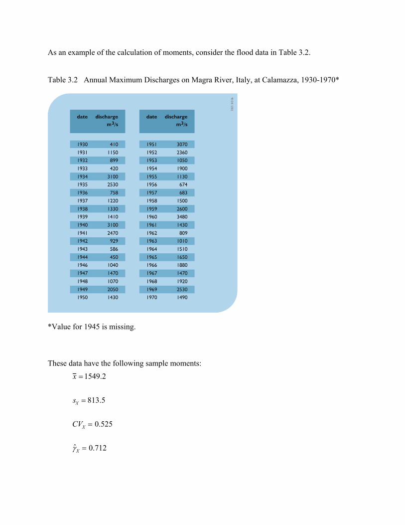
As an example of the calculation of moments, consider the flood data in Table 3.2. Table 3.2 Annual Maximum Discharges on Magra River, Italy, at Calamazza, 1930-1970*

*Value for 1945 is missing.

These data have the following sample moments: x =1549.2

sX = 813.5

CVX = 0.525

ˆ γ X = 0.712

As one can see, the data are positively skewed and have a relatively large coefficient of variance.

When discussing the accuracy of sample estimates, two quantities are often considered, bias and

variance. An estimator θ̂ of a known or unknown quantity θ is a function of the observed

values of the random variable X, say in n different time periods, X1, . . . , Xn, that will be

available to estimate the value of θ ; θ̂ may be written θ̂ [X1, X2, . . . , Xn] to emphasize that θ̂

itself is a random variable. Its value depends on the sample values of the random variable that

will be observed. An estimator θ̂ of a quantity θ is biased if ˆ[ ]E θ θ≠ and unbiased if

ˆ[ ]E θ θ= . The quantity ˆ{ [ ] }E θ θ− is generally called the bias of the estimator.

An unbiased estimator has the property that its expected value equals the value of the quantity to

be estimated. The sample mean is an unbiased estimate of the population mean µX because

[ ]1 1

1 1n n

i ii i

E X E X E Xn n Xµ

= =

⎡ ⎤⎡ ⎤ = =⎢ ⎥⎣ ⎦ ⎢ ⎥⎣ ⎦

∑ ∑ = (3.40)

The estimator 2XS of the variance of X is an unbiased estimator of the true variance 2

Xσ for

independent observations (Benjamin and Cornell, 1970):

2 2X XE S σ⎡ ⎤ =⎣ ⎦ (3.41)

However, the corresponding estimator of the standard deviation, SX, is in general a biased

estimator of σx because

[ ] ≠XE S Xσ (3.42)

The second important statistic often used to assess the accuracy of an estimator θ̂ is the variance

of the estimator Var ( )θ̂ , which equals ( )2ˆ ˆE Eθ θ⎧ ⎫⎡ ⎤−⎨ ⎬⎣ ⎦⎩ ⎭. For the mean of a set of independent

observations, the variance of the sample mean is

( )2

Var XXn

σ= (3.43)

It is common to call /x nσ the standard error of x rather than its standard deviation. The

standard error of an average is the most commonly reported measure of the precision.

The bias measures the difference between the average value of an estimator and the quantity to

be estimated. The variance measures the spread or width of the estimator’s distribution. Both

contribute to the amount by which an estimator deviates from the quantity to be estimated.

These two errors are often combined into the mean square error. Understanding that θ is fixed,

and the estimator θ̂ is a random variable, the mean squared error is the expected value of the

squared distance (error) between the two:

xx

( ) ( ) { } ( )2 22ˆ ˆ ˆ ˆ ˆMSE E E E Eθ θ θ θ θ θ θ⎧ ⎫⎡ ⎤ ⎡ ⎤ ⎡ ⎤= − = − + −⎨ ⎬⎢ ⎥ ⎣ ⎦ ⎣ ⎦⎣ ⎦ ⎩ ⎭[ ] ( )2 ˆBias Var θ= + (3.44)

where [Bias] is ( )ˆE θ θ− . Equation 3.44 shows that the MSE, equal to the expected average

squared deviation of the estimator θ̂ from the true value of the parameter θ, can be computed as

the bias squared plus the variance of the estimator. MSE is a convenient measure of how closely

θ̂ approximates θ because it combines both bias and variance in a logical way.

Estimation of the coefficient of skewness γx provides a good example of the use of the MSE for

evaluating the total deviation of an estimate from the true population value. The sample estimate

ˆXγ of Xγ is often biased, has a large variance, and its absolute value was shown by Kirby

(1974) to be bounded by the square root of the sample size n.

ˆ| |X nγ ≤ (3.45)

The bounds do not depend on the true skew γX. However, the bias and variance of ˆXγ do

depend on the sample size and the actual distribution of X. Table 3.3 contains the expected value

and standard deviation of the estimated coefficient of skewness ˆX

γ when X has either a normal

distribution, for which γX = 0, or a gamma distribution with γX = 0.25, 0.50, 1.00, 2.00, or 3.00.

These values are adapted from Wallis et al. (1974 a,b) who employed moment estimators slightly

different than those in Equation 3.39.

For the normal distribution, [ ]XˆE γ = 0 and Var[ ]Xγ̂ ≅ 5/n. In this case, the skewness estimator

is unbiased but highly variable. In all the other cases in Table 3.3 it is also biased.

Table 3.3 Sampling Properties of Coefficient of Skewness Estimator

Source: Wallis, et al. (1974b) who divided just by n in the estimators of the moments, whereas in Equations 3.39b and 3.39c we use the generally adopted coefficients of 1/(n-1) and n/(n-1)(n-2) for the variance and skew.

To illustrate the magnitude of these errors, consider the mean square error of the skew estimator

ˆXγ calculated from a sample of size 50 when X has a gamma distribution with γX = 0.50, a

reasonable value for annual streamflows. The expected value of ˆXγ is 0.45; its variance equals

(0.37)2, its standard deviation squared. Using Equation 3.44, the mean square error of ˆXγ is

( ) ( ) ( )2 2ˆMSE 0.45 0.50 0.37 0.0025 0.1369Xγ = − + = + = 0.139 ≅ 0.14 (3.46)

An unbiased estimate of γX is simply (0.50/0.45) ˆXγ . Here the estimator provided by Equation

3.39 has been scaled to eliminate bias. This unbiased estimator has a mean squared error of

( )2

2ˆ0.50 0.500.50 0.50 (0.37) 0.1690.48 0.45

XMSEγ⎛ ⎞ ⎡ ⎤⎛ ⎞= − + =⎜ ⎟ ⎜ ⎟⎢ ⎥⎝ ⎠⎣ ⎦⎝ ⎠

≅ 0.17 (3.47)

The mean square error of the unbiased estimator of ˆXγ is larger than the mean square error of

the biased estimate. Unbiasing ˆXγ results in a larger mean square error for all the cases listed in

Table 3.3 except for the normal distribution for which γX = 0, and the gamma distribution with γX

= 3.00.

As shown here for the skew coefficient, biased estimators often have smaller mean square errors

than unbiased estimators. Because the mean square error measures the total average deviation of

an estimator from the quantity being estimated, this result demonstrates that the strict or

unquestioning use of unbiased estimators is not advisable. Additional information on the

sampling distribution of quantiles and moments is contained in Stedinger et al. (1993).

2.4 L-Moments and their estimators

L-moments are another way to summarize the statistical properties of hydrologic data based on

linear combinations of the original sample (Hosking, 1990). Recently, hydrologists have found

that regionalization methods (to be discussed in Section 5) using L-moments are superior to

methods using traditional moments (Hosking and Wallis, 1997; Stedinger and Lu, 1995). L-

moments have also proved useful for construction of goodness-of-fit tests (Hosking et al., 1985,

Chowdhury et al., 1991; Fill and Stedinger, 1995), measures of regional homogeneity and

distribution selection methods (Vogel and Fennessey, 1993; Hosking and Wallis, 1997).

The first L-moment designated as λ1 is simply the arithmetic mean:

λ1 = E [ X ] (3.48)

Now let X(i|n) be the ith largest observation in a sample of size n (i = n corresponds to the largest).

Then, for any distribution, the second L-moment, λ2, is a description of scale based upon the

expected difference between two randomly selected observations.

λ2 = (1/2) E[ X(2|1) - X(1|2) ] (3.49)

Similarly, L-moment measures of skewness and kurtosis use three and four randomly selected

observations, respectively.

λ3 = (1/3) E[ X(3|3) - 2 X(2|3) + X(1|3) ] (3.50)

λ4 = (1/4) E[ X(4|4) - 3 X(3|4) + 3 X(2|4) - X(1|4) ] (3.51)

Sample estimates are often computed using intermediate statistics called probability weighted

moments (PWMs). The rth probability weighted moment is defined as

βr = E{ X [F(X)]r } (3.52)

where F(X) is the cumulative distribution function of X. Recommended (Landwehr et al., 1979;

Hosking and Wallis, 1995) unbiased PWM estimators, br, of βr are computed as

( )( ) ( )( ) ( )

on

1 ( j)j 2

n

2 jj 3

X1 ( 1)

n(n 1)1 1 2

n n 1 n 2

=

=

=

= −−

= −− −

∑

∑

b

b j X

b j −j X

(3.53)

These are examples of the general formula for computing estimators br of βr.

(i ) ( i )i i

i 1 i1 1/ /1 11= =

−⎛ ⎞ ⎛ ⎞ ⎛ ⎞ ⎛ ⎞= =⎜ ⎟ ⎜ ⎟ ⎜ ⎟ ⎜ ⎟+ ++⎝ ⎠ ⎝ ⎠ ⎝ ⎠ ⎝ ⎠

∑ ∑n n

rr r

n nb X X

r r r rn r

(3.54)

for r = 1, . . . , n–1.

L-moments are easily calculated in terms of PWMs using

λ1 = β0

λ2 = 2β1 − β0

λ3 = 6β2 − 6β1 + β0

λ4 = 20 β3 − 30β2 + 12β1 β0 (3.55)

Wang (1997) provides formulas for directly calculating L-moment estimators, b, of β. Measures

of the coefficient of variation, skewness, and kurtosis of a distribution can be computed with L-

moments, as they can with traditional product moments. Whereas skew primarily measures the

asymmetery of a distribution, the kurtosis is an additional measure of the thickness of the extreme

tails. Kurtosis is particularly useful for comparing symmetric distributions that have a skewness

coefficient of zero. Table 3.4 provides definitions of the traditional coefficient of

variation, coefficient of skewness, and coefficient of kurtosis, as well as the L-moment, L-

coefficient of variation, L-coefficient of skewness, and L-coefficient of kurtosis.

Table 3.4 Definitions of Dimensionless Product-Moment and L-Moment Ratios

The flood data in Table 3.2 can be used to provide an example of L-moments. Equation 3.53

yields estimates of the first three Probability Weighted Moments

b0 = 1,549.20

b1 = 1003.89

b2 = 759.02 (3.56)

Recall b0 is just the sample average x . The sample L-moments are easily calculated using the

probability weighted moments. One obtains

ˆ λ 1 = b0 = 1,549

ˆ λ 2 = 2b1 − b0 = 458

ˆ λ 3 = 6b2 − 6b1 + b0 = 80 (3.57)

Thus the sample estimates of the L-Coefficient of Variation, t2, and L-Coefficient of Skewness,

t3, are

t2 = 0.295

t3 = 0.174 (3.58)

3. Distributions of random events

A frequent task in water resources planning is the development of a model of some probabilistic

or stochastic phenomena such as streamflows, flood flows, rainfall, temperatures, evaporation,

sediment or nutrient loads, nitrate or organic compound concentrations, or water demands. This

often requires that one fit a probability distribution function to a set of observed values of the

random variable. Sometimes, one’s immediate objective is to estimate a particular quantile of

the distribution, such as the 100-year flood. 50-year 6-hour-rainfall depth, or the minimum 7-

day-average expected once-in-10-year flow. Then the fitted distribution can supply an estimate

of that quantity. In a stochastic simulation, fitted distributions are used to generate possible

values of the random variable in question.

Rather than fitting a reasonable and smooth mathematical distribution, one could use the

empirical distribution represented by the data to describe the possible values a random variable

may assume in the future and their frequency. In practice, the true mathematical form for the

distribution that describes the events is not known. Moreover, even if it was, its functional form

may have too many parameters to be of much practical use. Thus using the empirical

distribution represented by the data itself has substantial appeal.

Generally the free parameters of the theoretical distribution are selected (estimated) so as to

make the fitted distribution consistent with the available data. The goal is to select a physically

reasonable and simple distribution to describe the frequency of the events of interest, to estimate

that distribution's parameters, and ultimately to obtain quantiles, performance indices and risk

estimates of satisfactory accuracy for the problem at hand. Use of a theoretical distribution has

several advantages over use of the empirical distribution:

1. It presents a smooth interpretation of the empirical distribution. As a result quantiles,

performance indices, and other statistics computed using the fitted distribution should

be more accurate than those computed with the empirical distribution.

2. It provides a compact and easy-to-use representation of the data.

3. It is likely to provide a more realistic description of the range of values that the

random variable may assume and their likelihood; for example, by using the

empirical distribution one implicitly assumes that no values larger or smaller than the

sample maximum or minimum can occur. For many situations this is unreasonable.

4. Often one needs to estimate the likelihood of extreme events that lie outside of the

range of the sample (either in terms of x values or in terms of frequency); such

extrapolation makes little sense with the empirical distribution.

5. In many cases one is not interested in the values of a random variable X, but instead is

interested in derived values of variables Y that are functions of X. This could be a

performance function for some system. If Y is the performance function, interest

might be primarily in its mean value E[Y], or the probability some standard is

exceeded, Pr{Y > standard}. For some theoretical X-distributions, the resulting Y-

distribution may be available in closed form making the analysis rather simple. (The

normal distribution works with linear models, the lognormal distribution with product

models, and the gamma distribution with queuing systems.)

This section provides a brief introduction to some useful techniques for estimating the

parameters of probability distribution functions and for determining if a fitted distribution

provides a reasonable or acceptable model of the data. Subsections are also included on families

of distributions based on the normal, gamma and generalized-extreme-value distributions. These

three families have found frequent use in water resource planning (Kottegoda and Rosso, 1997).

3.1 Parameter estimation

Given a set of observations to which a distribution is to be fit, one first selects a distribution

function to serve as a model of the distribution of the data. The choice of a distribution may be

based on experience with data of that type, some understanding of the mechanisms giving rise to

the data, and/or examination of the observations themselves. One can then estimate the

parameters of the chosen distribution and determine if the fitted distribution provides an

acceptable model of the data. A model is generally judged to be unacceptable if it is unlikely

that one could have observed the available data were they actually drawn from the fitted

distribution.

In many cases, good estimates of a distribution’s parameters are obtained by the maximum-

likelihood-estimation procedure. Give a set of n independent observations {x1, . . . , xn} of a

continuous random variable X, the joint probability density function for the observations is

( ) ( ) ( ) ( )2 1 1 21 3 nX ,X , X X n X X X nf ,... x , . . . , x | f x | f x | . . . f x |θ θ θ= ⋅ θ (3.59)

where θ is the vector of the distribution’s parameters.

The maximum likelihood estimator of θ is that vector θ which maximizes Equation 3.59 and

thereby makes it as likely as possible to have observed the values {x1, . . . , xn}.

Considerable work has gone into studying the properties of maximum likelihood parameter

estimates. Under rather general conditions, asymptotically the estimated parameters are

normally distributed, unbiased, and have the smallest possible variance of any asymptotically

unbiased estimator (Bickel and Doksum, 1977). These, of course, are asymptotic properties,

valid for large sample sizes n. Better estimation procedures, perhaps yielding biased parameter

estimates, may exist for small sample sizes. Stedinger (1980) provides such an example. Still,

maximum likelihood procedures are recommended with moderate and large samples, even

though the iterative solution of nonlinear equations is often required.

An example of the maximum likelihood procedure for which closed-form expressions for the

parameter estimates are obtained is provided by the lognormal distribution. The probability

density function of a lognormally distributed random variable X is

fX x( )=1

x 2πσ 2exp −

12σ 2 ln(x) − µ[ 2⎧

⎨ ⎩

⎫] ⎬ ⎭ (3.60)

Here the parameters µ and σ2 are the mean and variance of the logarithm of X, and not of X itself.

Maximizing the logarithm of the joint density for {x1, . . . , xn} is more convenient than

maximizing the joint probability density itself. Hence the problem can be expressed as the

maximization of the log-likelihood function

( )1

ln ,n

ii

L f x=

⎡ ⎤= ⎣ ⎦∏ µ σ

(1

ln ,n

ii

f x=

= ∑ )µ σ (3.61)

( ) ( ) ( )2

21 1

1ln 2 ln2

n n

i ii i

x n ln x= =

⎡ ⎤= − − − −⎣ ⎦∑ ∑π σ µσ

The maximum can be obtained by equating to zero the partial derivatives ∂L/∂µ and ∂L/∂σ

whereby one obtains:

( )21

10 lnn

ii

L x µµ σ =

∂⎡ ⎤= = −⎣ ⎦∂ ∑

(3.62)

( )2

31

10 lnn

ii

L n x µσ σ σ =

∂⎡ ⎤= = − + −⎣ ⎦∂ ∑

These equations yield the estimators

( )1

1ˆ lnn

ii

xn

µ=

= ∑

(3.63)

( )2

2

1

1ˆ ˆlnn

ii

xn

σ µ=

⎡ ⎤= −⎣ ⎦∑

The second-order conditions for a maximum are met and these values maximize Equation 3.59.

It is useful to note that if one defines a new random variable Y = ln(X), then the maximum

likelihood estimates of the parameters µ and σ2, which are the mean and variance of the Y

distribution, are the sample estimates of the mean and variance of Y:

ˆ yµ =

(3.64)

2 2ˆ [( 1) / ] Yn n sσ = −

The correction [(n-1)/n] in this last equation is often neglected.

The second commonly used parameter estimation procedure is the method of moments. The

method of moments is often a quick and simple method for obtaining parameter estimates for

many distributions. For a distribution with m = 1, 2, or 3 parameters, the first m moments of

postulated distribution in Equations 3.34, 3.35 and 3.37 are equated to the estimates of those

moments calculated using Equations 3.39. The resulting nonlinear equations are solved for the

unknown parameters.

For the lognormal distribution, the mean and variance of X as a function of the parameters µ and

σ are given by

21exp 2Xµ µ σ⎛ ⎞= +⎜ ⎟

⎝ ⎠

(3.65)

( ) ( )2 2exp 2 + exp 1X⎡ ⎤= −⎣ ⎦σ µ σ σ 2

Substituting x for µX and 2xs for 2

Xσ and solving for µ and σ2 one obtains

ˆ σ 2 = ln 1+ sX2 / x 2( )

(3.66)

ˆ µ = lnx

1 + sX2 / x 2

⎛

⎝ ⎜

⎞

⎠ ⎟ = ln x −

12

ˆ σ 2

The data in Table 3.2 provide an illustration of both fitting methods. One can easily compute the

sample mean and variance of the logarithms of the flows to obtain

ˆ µ = 7.202

(3.67) ˆ σ 2 = 0.3164 = (0.5625)2

Alternatively, the sample mean and variance of the flows themselves are

x = 1549.2

(3.68)

sX2 = 661,800 = (813.5)2

Substituting those two values in Equation 3.66 yields

ˆ µ = 7.224

(3.69)

ˆ σ 2 = 0.2435 = (0.4935)2

Method of moments and maximum likelihood are just two of many possible estimation methods.

Just as method of moments equates sample estimators of moments to population values and

solves for a distribution’s parameters, one can simply equate L-moment estimators to population

values and solve for the parameters of a distribution. The resulting method of L-moments has

received considerable attention in the hydrologic literature (Landwehr et al. 1978, Hosking et al.

1985; Hosking et al. 1987; Hosking, 1990; Wang, 1997). It has been shown to have significant

advantages when used as a basis for regionalization procedures that will be discussed in Section

5 (Lettenmaier et al., 1987; Stedinger and Lu, 1995; Hosking and Wallis, 1997).

Bayesian procedures provide another approach that is related to maximum likelihood estimation.

Bayesian inference employs the likelihood function to represent the information in the data.

That information is augmented with a prior distribution that describes what is known about

constraints on the parameters and their likely values beyond the information provided by the

recorded data available at a site. The likelihood function and the prior probability density

function are combined to obtain the probability density function that describes the posterior

distribution of the parameters:

fθ( θ | x1, x2, …, xn) ∝ fX( x1, x2, …, x n |θ) ξ(θ) (3.70)

The term ∝ means “proportional to” and ξ(θ) is the probability density function for the prior

distribution for θ (Kottegoda and Rosso, 1997). Thus, except for a constant of proportionality,

the probability density function describing the posterior distribution of the parameter vector θ is

equal to the product of the likelihood function fX( x1, x2, …, x n |θ ) and the probability density

function for the prior distribution ξ(θ) for θ.

Advantages of the Bayesian approach are that it allows the explicit modeling of uncertainty in

parameters (Stedinger, 1997; Kuczera, 1999), and provides a theoretically consistent framework

for integrating systematic flow records with regional and other hydrologic information (Vicens

et al., 1975; Stedinger, 1983; and Kuczera, 1983). Martins and Stedinger (2000) illustrate how

a prior distribution can be used to enforce realistic constraints upon a parameter as well as

providing a description of its likely values. In their case use of a prior of the shape parameter κ

of a generalized extreme value (GEV) distribution (discussed in Section 3.6) allowed definition

of generalized maximum likelihood estimators that over the κ-range of interest performed

substantially better than maximum likelihood, moment, and L-moment estimators.

While Bayesian methods have been available for decades, the computational challenge posed by

the solution of Equation 3.70 has been an obstacle to their use. Solutions to Equation 3.70 have

been available for special cases such as normal data, and binomial and Poisson samples (Raiffa

and Schlaifier, 1961; Benjamin and Cornell, 1970; Zellner, 1971). However, a new and very

general set of Markov Chain Monte Carlo (MCMC) procedures (discussed in Section 7.2) allow

numerical computation of the posterior distributions of parameters for a very broad class of

models (Gilks et al., 1996). As a result, Bayesian methods are now becoming much more

popular, and are the standard approach for many difficult problems that are not easily addressed

by traditional methods (Gelman et al., 1995; Carlin and Louis, 2000). The use of Monte Carlo

Bayesian methods in flood frequency analysis, rainfall-runoff modeling, and evaluation of

environmental pathogen concentrations are illustrated by Wang (2001), Bates and Campbell

(2001) and Crainiceanu et al. (2002) respectively.

Finally, a simple method of fitting flood frequency curves is to plot the ordered flood values on

special probability paper and then to draw a line through the data (Gumbel, 1958). Even today,

that simple method is still attractive when some of the smallest values are zero or unusually

small, or have been censored as will be discussed in Section 4 (Kroll and Stedinger, 1996).

Plotting the ranked annual maximum series against a probability scale is always an excellent and

recommended way to see what the data look like and for determining whether a fitted curve is or

is not consistent with the data (Stedinger et al., 1993).

Statisticians and hydrologists have investigated which of these methods most accurately

estimates the parameters themselves or the quantiles of the distribution (Stedinger, 1997). One

also needs to determine how accuracy should be measured. Some studies have used average

squared deviations, some have used average absolute weighted deviations with different weights

on under- and over-estimation, and some have used the squared deviations of the log-quantile

estimator (Slack et al., 1975; Kroll and Stedinger, 1996). In almost all cases, one is also

interested in the bias of an estimator, which is the average value of the estimator minus the true

value of the parameter or quantile being estimated. Special estimators have been developed to

compute design events that on average are exceeded with the specified probability, and have the

anticipated risk of being exceeded (Beard, 1960, 1997; Rasmussen and Rosbjerg, 1989, 1991a,b;

Stedinger, 1997; Rosbjerg and Madsen, 1998).

3.2 Model adequacy

After estimating the parameters of a distribution, some check of model adequacy should be

made. Such checks vary from simple comparisons of the observations with the fitted model

using graphs or tables, to rigorous statistical tests. Some of the early and simplest methods of

parameter estimation were graphical techniques. Although quantitative techniques are generally

more accurate and precise for parameter estimation, graphical presentations are invaluable for

comparing the fitted distribution with the observations for the detection of systematic or

unexplained deviations between the two. The observed data will plot as a straight line on

probability graph paper if the postulated distribution is the true distribution of the observation. If

probability graph paper does not exist for the particular distribution of interest, more general

techniques can be used.

Let x(i) be the ith largest value in a set of observed values{xi} so that x(1) ≤ x(2) ≤ . . . ≤ x(n). The

random variable X(i) provides a reasonable estimate of the pth quantile xp of the true distribution

of X for p = i/(n+1). In fact, if one thinks of the cumulative probability Ui associated with the

random variable X(i), Ui = FX(X(i)), then if the observations X(i) are independent, the Ui have a

beta distribution (Gumbel, 1958) with probability density function

fUi (u) =n!

(i− 1) !(n −1) !ui−1(1− u)n− i 0≤ u ≤1 (3.71)

This beta distribution has mean and variance of

[ ]1i

iE Un

=+

(3.72a)

and

2

( 1)( )( 1) ( 2)i

i n iVar Un n

− +=

+ + (3.72b)

A good graphical check of the adequacy of a fitted distribution G(x) is obtained by plotting the

observations x(i) versus G-1[i/(n + 1)] (Wilk and Gnanadesikan, 1968). Even if G(x) exactly

equaled the true X-distribution FX[x], the plotted points will not fall exactly on a 45-degree line

through the origin of the graph. This would only occur if FX[x(i)] exactly equaled i/(n+1) and

therefore each x(i) exactly equaled FX-1[i/(n+1)].

An appreciation for how far an individual observation x(i) can be expected to deviate from

G-1[i/(n+1)] can be obtained by plotting G-1[ui(0.75)] and G-1[ui

(0.25)], where ui(0.75) and ui

(0.25) are

the upper and lower quartiles of the distribution of Ui obtained from integrating the probability

density function in Equation 3.71. The required incomplete beta function is also available in

many software packages, including Microsoft Excel. Stedinger et al. (1993) show that u(1) and (1

– u(1)) fall between 0.052/n and 3(n+1) with a probability of 90 percent, thus illustrating the great

uncertainty associated with those values.

Figures 3.2a and 3.2b illustrate the use of this quantile-quantile plotting technique by displaying

the results of fitting a normal and a lognormal distribution to the annual maximum flows in Table

3.2 for the Magra River, Italy, at Calamazza for the years 1930-1970. The observations of X(i),

given in Table 3.2, are plotted on the vertical axis against the quantiles

G-1[i/(n+1)] on the horizontal axis.

(a)

(b)

Figure 3.2. Plots of annual maximum discharges of Magra River, Italy, versus quantiles of fitted

(a) normal and (b) lognormal distributions.

A probability plot is essentially a scatter plot of the sorted observations X(i) versus some

approximation of their expected or anticipated value, represented by G-1(pi), where, as suggested,

pi = i/(n+1). The pi values are called plotting positions. A common alternative to i/(n+1) is (i-

0.5)/n, which results from a probabilistic interpretation of the empirical distribution of the data.

Many reasonable plotting position formulas have been proposed based upon the sense in which

G-1(pi) should approximate X(i). The Weibull formula i/(n+1) and the Hazen formula (i-0.5)/n

bracket most of the reasonable choices. Popular formulas are summarized in Stedinger et al.

(1993), who also discuss the generation of probability plots for many distributions commonly

employed in hydrology.

Rigorous statistical tests are available for trying to determine whether or not it is reasonable to

assume that a given set of observations could have been drawn from a particular family of

distributions. Although not the most powerful of such tests, the Kolmogorov-Smirnov test

provides bounds within which every observation should lie if the sample is actually drawn from

the assumed distribution. In particular, for G = FX, the test specifies that

1 1( )

1Pr for every i 1ii iG C X G Cn n

− −⎡ −⎛ ⎞ ⎛ ⎞− ≤ ≤ + = −⎜ ⎟ ⎜ ⎟⎢ ⎥⎝ ⎠ ⎝ ⎠⎣ ⎦α α

⎤ α (3.73)

where Cα is the critical value of the test at significance level α. Formulas for Cα as a function of

n are contained in Table 3.5 for three cases: (1) when G is completely specified independent of

the sample’s values; (2) when G is the normal distribution and the mean and variance are

estimated from the sample with 2x and sx ; and (3) when G is the exponential distribution and the

scale parameter is estimated as 1/( )x . Chowdhury et al. (1991) provide critical values for the

Gumbel and generalized extreme value (GEV) distributions (Section 3.6) with known shape

parameter κ. For other distributions, the values obtained from Table 3.5 may be used to

construct approximate simultaneous confidence intervals for every X(i).

Figures 3.2 a and b contain 90% confidence intervals for the plotted points constructed in this

manner. For the normal distribution, the critical value of Cα equals

0.819 / ( n − 0.01+ 0.85 / n) , where 0.819 corresponds to α = 0.10. For n = 40, one computes

Cα = 0.127. As can be seen in Figure 3.2a, the annual maximum flows are not consistent with the

hypothesis that they were drawn from a normal distribution; three of the observations lie outside

the simultaneous 90% confidence intervals for all points. This demonstrates a statistically

significant lack of fit. The fitted normal distribution underestimates the quantiles corresponding

to small and large probabilities while overestimating the quantiles in an intermediate range. In

Figure 3.2b, deviations between the fitted lognormal distribution and the observations can be

attributed to the differences between FX(x(i)) and i/(n + 1). Generally, the points are all near the

45-degree line through the origin, and no major systematic deviations are apparent.

The Kolmogorov-Smirnov test conveniently provides bounds within which every observation on

a probability plot should lie if the sample is actually drawn from the assumed distribution, and

thus is useful for visually evaluating the adequacy of a fitted distribution. However, it is not the

most powerful test available for estimating which distribution a set of observations is likely to

have been drawn. For that purpose several other more analytical tests are available (Filliben,

1975; Hosking, 1990; Chowdhury et al., 1991; Kottegoda and Rosso, 1997).

Table 3.5 Critical Valuesα of Kolmogorov-Smirnov Statistic as a Function of Sample Size n

The Probability Plot Correlation test is a popular and powerful test of whether a sample has

been drawn from a postulated distribution, though it is often weaker than alternative tests at

rejecting thin-tailed alternatives (Filliben, 1975; Fill and Stedinger, 1995). A test with greater

power has a greater probability of correctly determining that a sample is not from the postulated

distribution. The Probability Plot Correlation Coefficient test employs the correlation r between

the ordered observations x(i) and the corresponding fitted quantiles wi = G-1

(pi), determined by

plotting positions pi for each x(i). Values of r near 1.0 suggest that the observations could have

been drawn from the fitted distribution: r measures the linearity of the probability plot providing

a quantitative assessment of fit. If x denotes the average value of the observations and w

denotes the average value of the fitted quantiles, then

r =x( i) − x ( ) w i − w ( )∑

x ( i) − x ( )2w i − w ( )∑∑

2⎛ ⎝

⎞ ⎠

⎡ ⎣ ⎢

⎤ ⎦ ⎥

0.5

(3.74)

Table 3.6 provides critical values for r for the normal distribution, or the logarithms of lognormal

variates, based upon the Blom plotting position that has pi = (i-3/8)/(n+1/4). Values for the

Gumbel distribution are reproduced in Table 3.7 for use with the Gringorten plotting position pi

= (i-0.44)/(n+0.12). The table also applies to logarithms of Weibull variates (Stedinger et al.,

1993). Other tables are available for the GEV (Chowdhury et al., 1991), the Pearson type 3

(Vogel and McMartins, 1991), and exponential and other distributions (D’Agostion and

Stephens, 1986).

Table 3.6. Lower Critical Values of the Probability Plot Correlation Test Statistic for the Normal

Distribution using pi = (i -3/8)/(n+1/4) (Vogel, 1987)

Table 3.7 Lower Critical Values of the Probability Plot Correlation Test Statistic for the Gumbel

Distribution using pi = (i -0.44)/(n+0.12) (Vogel, 1987)

Recently developed L-moment ratios appear to provide goodness-of-fit tests that are superior to

both the Kolmogorov-Smirnov and the Probability Plot Correlation test (Hosking, 1990;

Chowdhury et al., 1991; Fill and Stedinger, 1995). For normal data, the L-skewness estimator ˆ τ 3 (or t3) would have mean zero and Var[ ˆ τ 3 ] = (0.1866 + 0.8/n)/n, allowing construction of a

powerful test of normality against skewed alternatives using the normally distributed statistic

Z = t3 / 0.1866 + 0.8 / n( / n) (3.75)

with a reject region |Z| > zα/2.

Chowdhury et al. (1991) derive the sampling variance of the L-CV and L-skewness estimators

and as a function of κ for the GEV distribution. These allow construction of a test of

whether a particular data set is consistent with a GEV distribution with a regionally estimated

value of κ, or a regional κ and a coefficient of variation, CV. Fill and Stedinger (1995) show

2τ̂ 3τ̂

that the ˆ τ 3 L-skewness estimator provides a test for the Gumbel versus a general GEV

distribution using the normally distributed statistic

Z = ( ˆ τ 3 - 0.17)/ 0.2326 + 0.70 / n( / n) (3.76)

with a reject region |Z| > zα/2.

The literature is full of goodness-of-fit tests. Experience indicates that among the better tests

there is often not a great deal of difference (D’Agostion and Stephens, 1986). Generation of a

probability plot is most often a good idea because it allows the modeler to see what the data look

like and where problems occur. The Kolmogorov-Smirnov test helps the eye interpret a

probability plot by adding bounds to a graph illustrating the magnitude of deviations from a

straight line that are consistent with expected variability. One can also use quantiles of a beta

distribution to illustrate the possible error in individual plotting positions, particularly at the

extremes where that uncertainty is largest. The probability plot correlation test is a popular and

powerful goodness-of-fit statistic. Goodness-of-fit tests based upon sample estimators of the L-

skewness ˆ τ 3 for the normal and Gumbel distribution provide simple and useful tests that are not

based on a probability plot.

3.3 Normal and lognormal distributions

The normal distribution and its logarithmic transformation, the lognormal distribution, are

arguably the most widely used distributions in science and engineering. The density function of

a normal random variable is

fX (x) =1

2πσ 2exp −

12σ 2 (x − µ)2⎡

⎣ ⎢ ⎤ ⎦ ⎥ for – ∞ < X < + ∞ (3.77)

where µ and σ2 are equivalent to µX and σ X2 , the mean and variance of X. Interestingly, the

maximum likelihood estimators of µ and σ2 are almost identical to the moment estimates x and

2Xs .

The normal distribution is symmetric about its mean µX and admits values from - ∞ to + ∞. Thus

it is not always satisfactory for modeling physical phenomena such as streamflows or pollutant

concentrations, which are necessarily non-negative and have skewed distributions. A frequently

used model for skewed distributions is the lognormal distribution. A random variable X has a

lognormal distribution if the natural logarithm of X, ln(X), has a normal distribution. If X is

lognormally distributed, then by definition ln(X) is normally distributed, so that the density

function of X is

[ ]222

1 1 (( ) exp ( )22

Xd n xf x n x

dx⎧= − −⎨⎩ ⎭

ll µ

σπσ

)⎫⎬

[ ]222

1 1exp ( / )22

n xx

ησπσ

⎧ ⎫= −⎨ ⎬⎩ ⎭

l (3.78)

for x > 0 and µ = ln(η). Here η is the median of the X-distribution. The coefficient of skewness

for the 3-parameter lognormal distribution is given by

γ = 3 υ + υ3 where υ = [ exp(σ2) − 1 ]0.5 (8a.79)

A lognormal random variable takes on values in the range [0, +∞]. The parameter µ determines

the scale of the X-distribution whereas σ2 determines the shape of the distribution. The mean

and variance of the lognormal distribution are given in Equation 3.65. Figure 3.3 illustrates the

various shapes the lognormal probability density function can assume. It is highly skewed with a

thick right hand tail for σ > 1, and approaches a symmetric normal distribution as σ → 0. The

density function always has a value of zero at x = 0. The coefficient of variation and skew are

CVX = [exp (σ2) – 1]1/2

γX = 3 CVX + CVX3 (3.80)

The maximum likelihood estimates of µ and σ2 are given in Equation 3.63 and the moment

estimates in Equation 3.66. For reasonable-size samples, the maximum likelihood estimates

generally perform as well or better than the moment estimates (Stedinger, 1980).

Figure 3.3. Lognormal probability density functions with various standard deviations σ.

The data in Table 3.2 were used to calculate the parameters of the lognormal distribution that

would describe the flood flows. The results are reported in Equation 3.67. The two-parameter

maximum likelihood and method of moments estimators identify parameter estimates for which

the distribution skewness coefficients are 2.06 and 1.72, which is substantially greater than the

sample skew of 0.712.

A useful generalization of the two-parameter lognormal distribution is the shifted lognormal or

three-parameter lognormal distribution obtained when ln(X – τ) is described by a normal

distribution, and X ≥ τ. Theoretically, τ should be positive if for physical reasons X must be

positive; practically, negative values of τ can be allowed when the resulting probability of

negative values of X is sufficiently small.

Unfortunately, maximum likelihood estimates of the parameters µ, σ2, and τ are poorly behaved

because of irregularities in the likelihood function (Giesbrecht and Kempthorne, 1976). The

method of moments does fairly well when the skew of the fitted distribution is reasonably small.

A method that does almost as well as the moment method for low-skew distributions, and much

better for highly skewed distributions, estimates τ by:

ˆ τ =x(1)x(n) − ˆ x 0.50

2

x(1) + x(n) − 2 ˆ x 0.50 (3.81)

provided that x(1) + x(n) – 2 x̂ 0.50 > 0, where x(1) and x(n) are the smallest and largest observations

and 0.50x̂ is the sample median (Stedinger, 1980; Hoshi et al., 1984). If x(1) + x(n) - 0.50ˆ2x < 0,

the sample tends to be negatively skewed and a three-parameter lognormal distribution with a

lower bound cannot be fit with this method. Good estimates of µ and σ2 to go with ˆ τ in

Equation 3.81 are (Stedinger, 1980):

( )22

ˆˆˆ1 /x

xns x

τµτ

⎡ ⎤−⎢ ⎥=

⎢ ⎥+ −⎢ ⎥⎣ ⎦

l

( )

22

2ˆ 1

ˆxsn

x

⎡ ⎤⎢= +⎢ ⎥−⎣ ⎦

lστ

⎥ (3.82)

For the data in Table 3.2, Equation 3.82 yields the hybrid moment-of-moments estimates for the

3-parameter lognormal distribution. These estimates are µ̂ = 7.606, 2σ̂ = 0.1339 = (0.3659)2

and = – 600.1. τ̂

This distribution has a coefficient of skewness of 1.19, which is more consistent with the sample

skewness estimator than was the value obtained when a 2-parameter lognornal distribution was

fit to the data. Alternatively, one can estimate µ and σ2 by the sample mean and variance of

ln(X – ) which yields the hybrid maximum likelihood estimates of τ̂ µ̂ = 7.605, 0.1407 =

(0.3751)

2σ̂ =2 and again = – 600.1. τ̂

The two sets of estimates are surprisingly close in this instance. In this second case, the fitted

distribution has a coefficient of skewness of 1.22.

Natural logarithms have been used here. One could have just as well use base 10 common

logarithms to estimate the parameters; however, in that case the relationships between the log-

space parameters and the real-space moments change slightly (Stedinger et al., 1993, Eqn.

18.2.8).

3.4 Gamma distributions

The gamma distribution has long been used to model many natural phenomena, including daily,

monthly, and annual streamflows as well as flood flows (Bobee and Ashkar, 1991). For a

gamma random variable X,

fX (x) =β

Γ(α)βx( )α −1

e−βx βx ≥ 0

X =αµβ

22X =

ασβ

2 2X XCV= =γα

(3.83)

The gamma function, Γ(α), for integer α is (α - 1)!. The parameter α > 0 determines the shape

of the distribution; β is the scale parameter. Figure 3.4 illustrates the different shapes that the

probability density function for a gamma variable can assume. As α → ∞, the gamma

distribution approaches the symmetric normal distribution, whereas for 0 < α < 1, the distribution

has a highly asymmetric J-shaped probability density function whose value goes to infinity as x

approaches zero.

Figure 3.4. The gamma distribution function for various values of the shape parameter α.

The gamma distribution arises naturally in many problems in statistics and hydrology. It also has

a very reasonable shape for such nonnegative random variables as rainfall and streamflow.

Unfortunately, its cumulative distribution function is not available in closed form, except for

integer α, though it is available in many software packages including Microsoft Excel. The

gamma family includes a very special case: the exponential distribution is obtained when α = 1.

The gamma distribution has several generalizations (Bobee and Ashkar, 1991). If a constant τ is

subtracted from X so that (X − τ) has a gamma distribution, the distribution of X is a three-

parameter gamma. This is also called a Pearson type 3 distribution, because the resulting

distribution belongs to the third type of distributions suggested by the statistician Karl Pearson.

Another variation is the log Pearson type 3 distribution obtained by fitting the logarithms of X

with a Pearson type 3 distribution. The log Pearson distribution is discussed further in the next

section.

The method of moments may be used to estimate the parameters of the gamma distribution. For

the three-parameter gamma distribution

ˆ 2ˆX

X

sx⎛ ⎞

= − ⎜ ⎟⎝ ⎠

τγ

( )24ˆ

ˆX

=αγ

(3.84)

2ˆX Xs

=βγ

where 2 ˆ, , and X Xx s γ are estimates of the mean, variance, and coefficient of skewness of the

distribution of X (Bobee and Robitaille, 1977).

For the two-parameter gamma distribution,

( )2

2ˆ

x

xs

α =

(3.85)

2ˆ

x

xs

β =

Again the flood record in Table 3.2 can be used to illustrate the different estimation procedures.

Using the first three sample moments, one would obtain for the 3-parameter gamma distribution

the parameter estimates

ˆ τ = –735.6

ˆ α = 7.888

ˆ β = 0.003452 = 1/289.7

Using only the sample mean and variance yields the method of moment estimators of the

parameters of the 2-parameter gamma distribution (τ = 0)

ˆ α = 3.627 ˆ β = 0.002341 = 1/427.2

The fitted 2-parameter gamma distribution has a coefficient of skewness γ of 1.05 whereas the

fitted 3-parameter gamma reproduces the sample skew of 0.712. As occurred with the 3-

parameter lognormal distribution, the estimated lower bound for the 3-parameter gamma

distribution is negative ( ˆ τ = –735.6) resulting in a 3-parameter model that has a smaller skew

coefficient than was obtained with the corresponding 2-parameter model. The reciprocal of

is also reported. While has inverse x-units, 1/ is a natural scale parameter that has the

same units as x and thus can be easier to interpret.

ˆ β

ˆ β ˆ β

Studies by Thom (1958) and Matalas and Wallis (1973) have shown that maximum likelihood

parameter estimates are superior to the moment estimates. For the two-parameter gamma

distribution, Greenwood and Durand (1960) give approximate formulas for the maximum

likelihood estimates (also Haan, 1977). However, the maximum likelihood estimators are often

not used in practice because they are very sensitive to the smallest observations that sometimes

suffer from measurement error and other distortions.

When plotting the observed and fitted quantiles of a gamma distribution, an approximation to the

inverse of the distribution function is often useful. For |γ | ≤ 3, the Wilson-Hilferty

transformation

322 1

6 36N

Gxx γ γµ σ 2

γ γ

⎡ ⎤⎛ ⎞⎢= + + − −⎜ ⎟⎜ ⎟⎢ ⎥⎝ ⎠⎣ ⎦

⎥ (3.86)

gives the quantiles xG of the gamma distribution in terms of xN, the quantiles of the standard-

normal distribution. Here µ, σ, and γ are the mean, standard deviation, and coefficient of

skewness of xG. Kirby (1972) and Chowdhury and Stedinger (1971) discuss this and other more

complicated but more accurate approximations. Fortunately the availability of excellent

approximations of the gamma cumulative distribution function and its inverse in Microsoft Excel

and other packages has reduced the need for such simple approximations.

3.5 Log-Pearson type 3 distribution

The log-Pearson type 3 distribution (LP3) describes a random variable whose logarithms have a

Pearson type 3 distribution. This distribution has found wide use in modeling flood frequencies

and has been recommended for that purpose (IACWD, 1982). Bobee (1975) and Bobee and

Ashkar (1991) discuss the unusual shapes that this hybrid distribution may take allowing

negative values of β. The LP3 distribution has a probability density function given by

fX(x) = |β|{ β[ ln(x) – ξ]}α−1 exp{ – β[ln(x) – ξ] }/{ x Γ(α) } (3.87)

with α > 0, and β either positive or negative. For β < 0, values are restricted to the range 0 < x <

exp(ξ). For β > 0, values have a lower bound so that exp(ξ) < X. Figure 3.5 illustrates the

probability density function for the LP3 distribution as a function of the skew γ of the P3

distribution describing ln(X), with σlnX = 0.3. The LP3 density function for |γ | ≤ 2 can assume a

wide range of shapes with both positive and negative skews. For |γ | = 2, the log-space P3

distribution is equivalent to an exponential distribution function which decays exponentially as x

moves away from the lower bound (β > 0) or upper bound (β < 0): as a result the LP3

distribution has a similar shape. The space with –1 < γ may be more realistic for describing

variables whose probability density function becomes thinner as x takes on large values. For γ =

0, the 2-parameter lognormal distribution is obtained as a special case.

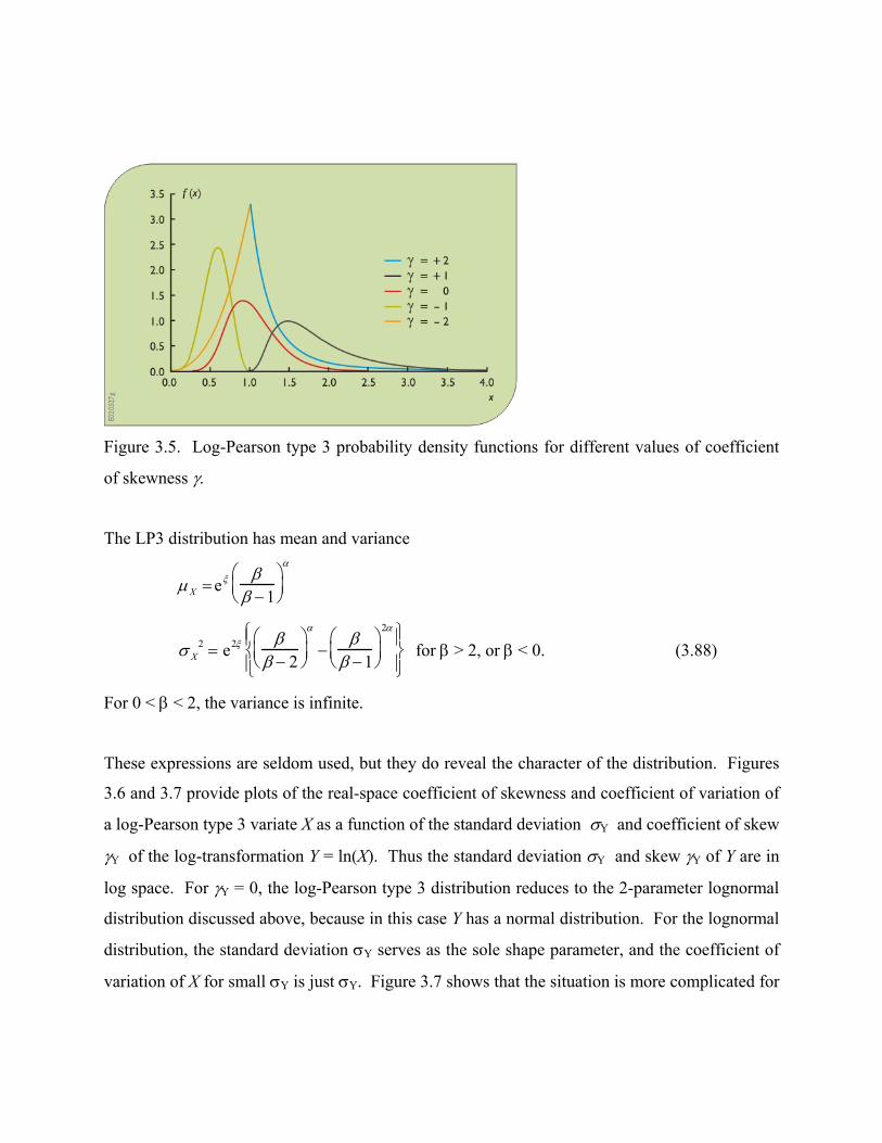
Figure 3.5. Log-Pearson type 3 probability density functions for different values of coefficient

of skewness γ.

The LP3 distribution has mean and variance

µ X = eξ β

β − 1⎛ ⎝ ⎜

⎞ ⎠ ⎟

α

σ X

2 = e2ξ ββ − 2

⎛ ⎝ ⎜

⎞ ⎠ ⎟

α

−β

β −1⎛ ⎝ ⎜

⎞ ⎠ ⎟

2α⎧ ⎨ ⎪

⎩ ⎪

⎫ ⎬ ⎪

⎭ ⎪ for β > 2, or β < 0. (3.88)

For 0 < β < 2, the variance is infinite.

These expressions are seldom used, but they do reveal the character of the distribution. Figures

3.6 and 3.7 provide plots of the real-space coefficient of skewness and coefficient of variation of

a log-Pearson type 3 variate X as a function of the standard deviation σY and coefficient of skew

γY of the log-transformation Y = ln(X). Thus the standard deviation σY and skew γY of Y are in

log space. For γY = 0, the log-Pearson type 3 distribution reduces to the 2-parameter lognormal

distribution discussed above, because in this case Y has a normal distribution. For the lognormal

distribution, the standard deviation σY serves as the sole shape parameter, and the coefficient of

variation of X for small σY is just σY. Figure 3.7 shows that the situation is more complicated for

the LP3 distribution. However, for small σY, the coefficient of variation of X is approximately

σY.

Figure 3.6. Real-space coefficient of skewness γX for LP3 distributed X as a function of log-

space standard deviation σY and coefficient of skewness γY where Y = ln(X).

Figure 3.7. Real-space coefficient of variation CVX for LP3 distributed X as a function of log-

space standard deviation σY and coefficient of skewness γY where Y = ln(X).

Again, the flood flow data in Table 3.2 can be used to illustrate parameter estimation. Using

natural logarithms, one can estimate the log-space moments with the standard estimators in

Equations 3.39 that yield: ˆ µ = 7.202

ˆ σ = 0.5625

ˆ γ = –0.337

For the LP3 distribution, analysis generally focuses on the distribution of the logarithms Y =

ln(X) of the flows, which would have a Pearson type 3 distribution with moments µY, σY and γY

(IACWD, 1982; Bobée and Ashkar, 1991). As a result, flood quantiles are calculated as

xp = exp{ µY + σY Kp[γY] } (3.89)

where Kp[γY] is a frequency factor corresponding to cumulative probability for skewness

coefficient γY. (Kp[γY] corresponds to the quantiles of a 3-parameter gamma distribution with

zero mean, unit variance, and skewness coefficient γY.)

Since 1967 the recommended procedure for flood frequency analysis by federal agencies in the

United States uses this distribution. Current guidelines in Bulletin 17B (IACWD, 1982) suggest

that the skew γY be estimated by a weighted average of the at-site sample skewness coefficient

and a regional estimate of the skewness coefficient. Bulletin 17B also includes tables of

frequency factors, a map of regional skewness estimators, checks for low outliers, confidence

interval formula, a discussion of expected probability, and a weighted-moments estimator for

historical data.

3.6 Gumbel and GEV distributions

The annual maximum flood is the largest flood flow during a year. One might expect that the

distribution of annual maximum flood flows would belong to the set of extreme value

distributions (Gumbel, 1958; Kottegoda and Rosso, 1997). These are the distributions obtained

in the limit, as the sample size n becomes large, by taking the largest of n independent random

variables. The Extreme Value (EV) type I distribution or Gumbel distribution has often been

used to describe flood flows. It has the cumulative distribution function:

FX(x) = exp{ – exp[ – (x-ξ)/α] } (3.90)

where ξ is the location parameter. It has a mean and variance of

µX = ξ + 0.5772 α

σX2 = π2α2/6 ≅ 1.645α2 (3.91)

Its skewness coefficient has the fixed value equal to γX = 1.1396.

The generalized extreme value (GEV) distribution is a general mathematical expression that

incorporates the type I, II, and III extreme value (EV) distributions for maxima (Gumbel, 1958;

Hosking et al., 1985). In recent years it has been used as a general model of extreme events

including flood flows, particularly in the context of regionalization procedures (NERC, 1975;

Stedinger and Lu, 1995; Hosking and Wallis, 1997). The GEV distribution has cumulative

distribution function:

FX(x) = exp{ – [ 1 – κ(x–ξ)/α]1/κ } for κ ≠ 0 (3.92)

From Equation 3.92 it is clear that for κ < 0 (the typical case for floods), x must be no less than

ξ + α/κ whereas for κ > 0, x must be no greater than ξ + α/κ (Hosking and Wallis, 1987). The

mean, variance, and skewness coefficient are (for κ > -1/3):

µX = ξ + (α/κ) [1 – Γ(1+κ)] ,

σX2 = (α/κ)2 { Γ(1+2κ) – [Γ(1+κ)]2 } (3.93)

γX = (Sign κ){ –Γ(1+3κ) + 3 Γ(1+κ) Γ(1+2κ) – 2[Γ(1+κ)] 3 } / {Γ(1+2κ) – [Γ(1+κ)]2]}3/2

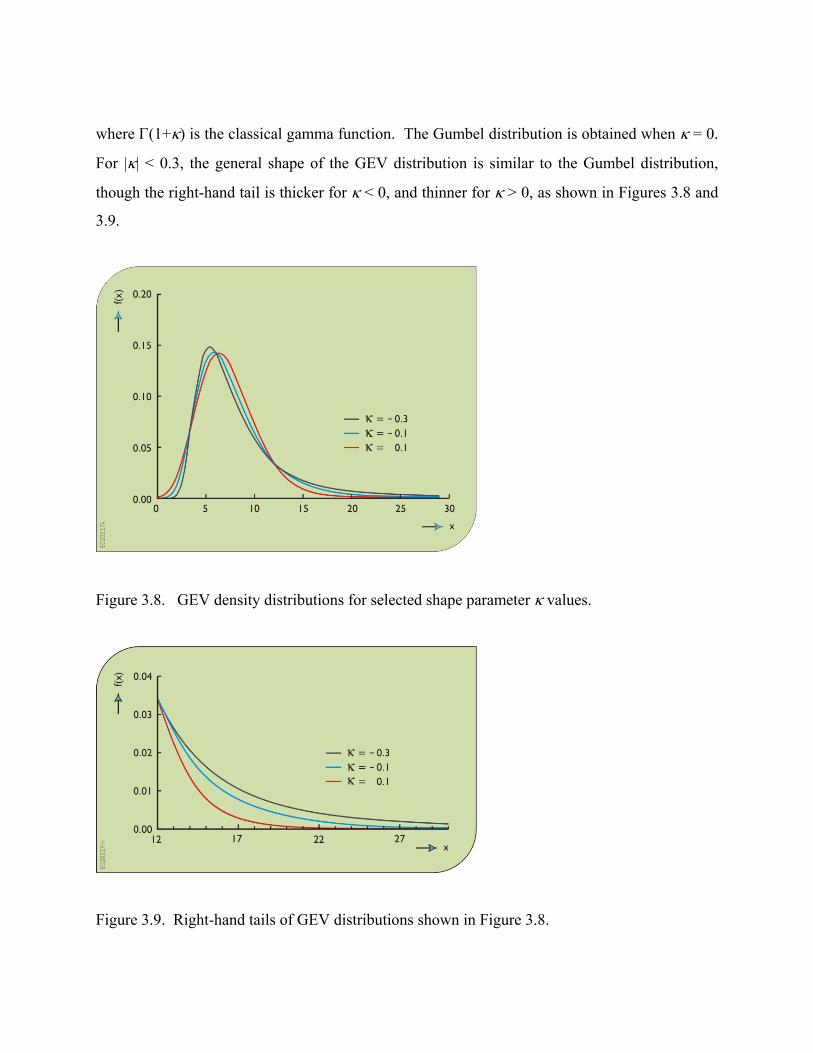
where Γ(1+κ) is the classical gamma function. The Gumbel distribution is obtained when κ = 0.

For |κ| < 0.3, the general shape of the GEV distribution is similar to the Gumbel distribution,

though the right-hand tail is thicker for κ < 0, and thinner for κ > 0, as shown in Figures 3.8 and

3.9.

Figure 3.8. GEV density distributions for selected shape parameter κ values.

Figure 3.9. Right-hand tails of GEV distributions shown in Figure 3.8.

The parameters of the GEV distribution are easily computed using L-moments and the

relationships (Hosking et al. (1985):

κ = 7.8590 c + 2.9554 c2

α = κ λ2 / [ Γ(1+κ) (1 - 2-κ) ] (3.94)

ξ = λ + ( α/κ [ Γ(1+κ) – 1 ]

where

c = 2 λ2/ (λ3 +3λ2) – ln(2)/ln(3) = [2 /(τ3 + 3)] – ln(2)/ln(3)

As one can see, the estimator of the shape parameter κ will depend only upon the L-skewness

estimator ˆ τ 3 . The estimator of the scale parameter α will then depend on the estimate of κ and

of λ2. Finally, one must also use the sample mean λ (Equation 3.48) to determine the estimate

of the location parameter ξ.

Using the flood data in Table 3.2 and the sample L-moments computed in Section 2, one obtains

first c = –0.000896 which yields ˆ κ = –0.007036, = 1165.20 and ˆ ξ ˆ α = 657.29.

The small value of the fitted κ parameter means that the fitted distribution is essentially a

Gumbel distribution. Again, ξ is a location parameter, not a lower bound, so its value resembles

a reasonable x value.

Madsen et al. (1997a) show that moment estimators can provide more precise quantile

estimators. Yet Martins and Stedinger, (2001) found that with occasional uninformative

samples, the MLE estimator of κ could be entirely unrealistic resulting in absurd quantile

estimators. However the use of a realistic prior distribution on κ yielded better generalized

maximum likelihood estimators (GLME) than moment and L-moment estimators over the range

of κ of interest.

The generalized maximum likelihood estimators (GMLE) are obtained my maximizing the log-

likelihood function, augmented by a prior density function on κ. A prior distribution that

reflects general world-wide geophysical experience and physical realism is in the form of a beta

distribution:

π(κ) = Γ (p) Γ(q) (0.5 + κ)p-1

(0.5 – κ) q-1

/ Γ(p+q) (3.95) for – 0.5 < κ < + 0.5 with p = 6 and q = 9. Moreover, this prior assigns reasonable probabilities

to the values of κ within that range. For κ outside the range – 0.4 to + 0.2 the resulting GEV

distributions do not have density functions consistent with flood flows and rainfall (Martins and

Stedinger, 2000). Other estimators implicitly have similar constraints. For example, L-

moments restricts κ to the range κ > – 1, and the method of moments estimator employs the

sample standard deviation so that κ > – 0.5. Use of the sample skew introduces the constraint

that κ > – 0.3. Then given a set of independent observations {x1, …, xn } drawn for a GEV

distribution, the generalized likelihood function is

ln{ L(ξ,α,,κ | x1, … xn )} = −n ln(α ) +1κ

−1⎛ ⎝

⎞ ⎠ ln yi( )− yi( )1

κ⎡ ⎣ ⎢

⎤ ⎦ ⎥

i=1

n

∑ + ln[π(κ)]

with

yi = [ 1 – (κ/α)(xi – ξ) ] (3.96)

For feasible values of the parameters, yi is greater than 0 (Hosking et al., 1985). Numerical

optimization of the generalized likelihood function is often aided by the additional constraint that

min{ y1, …,yn } ≥ ε for some small ε > 0 so as to prohibit the search generating infeasible values

of the parameters for which the likelihood function is undefined. The constraint should not be

binding at the final solution.

The data in Table 3.2 again provide a convenient data set for illustrating parameter estimators.

The L-moment estimators were used to generate an initial solution. Numerical optimization of

the likelihood function Equation 3.96 yielded the maximum likelihood estimators of the GEV

parameters: ˆ κ = -0.0359. ˆ ξ = 1165.4 and ˆ α = 620.2.

Similarly, use of the geophysical prior (Equation 3.95) yielded the generalized maximum

likelihood estimators ˆ κ = -0.0823, ˆ ξ = 1150.8 and α̂ = 611.4. Here the record length of 40

years is too short to reliably define the shape parameter κ so that result of using the prior is to

increase κ slightly toward the mean of the prior. The other two parameters adjust accordingly.

3.7 L-moment diagrams This Section 3 has presented several families of distributions. The L-moment diagram in Figure

3.10 illustrates the relationships between the L-kurtosis (τ3) and L-skewness (τ2) for a number of

distributions often used in hydrology. It shows that distributions with the same coefficient of

skewness still differ in the thickness of their tails. This thickness is described by their kurtosis.

Tail shapes are important if an analysis is sensitive to the likelihood of extreme events.

The normal and Gumbel distributions have a fixed shape and thus are presented by single points

that fall on the Pearson type 3 (P3) curve for γ = 0, and the generalized extreme value (GEV)

curve for κ = 0, respectively. The L-kurtosis / L-skewness relationships for the 2-parameter and

3-parameter gamma or P3 distributions are identical, as they are for the 2-parameter and 3-

parameter lognormal distributions. This is because the addition of a location parameter does not

change the range of fundamental shapes that can be generated. However, for the same skewness

coefficient, the lognormal distribution has a larger kurtosis than the gamma or P3 distribution

and thus assigns larger probabilities to the largest events.

As the skewness of the lognormal and gamma distributions approaches zero, both distributions

become normal and their kurtosis/skewness relationships merge. For the same L-skewness, the

L-kurtosis of the GEV distribution is generally larger than that of the lognormal distribution. For

positive κ yielding almost symmetric or even negatively skewed GEV distributions, the GEV has

a smaller kurtosis than the 3-parameter lognormal distribution. The latter can be negatively

skewed when τ is used as an upper bound.

Figurer 3.10 also includes the three-parameter generalized Pareto distribution, whose cdf is:

FX(x) = 1 – [ 1 – κ(x-ξ)/α]1/κ (3.97) (Hosking and Wallis, 1997). For κ = 0 it corresponds to the exponential distribution (gamma

with α = 1). This point is where the Pareto and P3 distribution L-kurtosis/L_skewness lines

cross. The Pareto distribution becomes increasing more skewed for κ < 0, which is the range of

interest in hydrology. The generalized Pareto distribution with κ < 0 is often used to describe

peaks-over-a-threshold and other variables whose density function has its maximum at their

lower bound. In that range for a given L-skewness, the Pareto distribution always has a larger

kurtosis than the gamma distribution. In these cases the α parameter for the gamma distribution

would need to be in the range 0 < α < 1, so that both distributions would be J-shaped.

As shown in Figure 3.10, the GEV distribution has a thicker right-hand tail than either the

gamma/Pearson type 3 distribution or the lognormal distribution.

Figure 3.10. Relationships between L-skewness and L-kurtosis for various distributions. 4. Analysis of censored data

There are many instances in water resources planning where one encounters censored data. A

data set is censored if the values of observations that are outside a specified range of values are

not specifically reported (David, 1981). For example, in water quality investigations many

constituents have concentrations that are reported as < T, where T is a reliable detection threshold

(MacBerthouex and Brown, 2002). Thus the concentration of the water quality variable of

interest was too small to be reliably measured. Likewise, low-flow observations and rainfall

depths can be rounded to or reported as zero. Several approaches are available for analysis of

censored data sets including probability plots and probability-plot regression, conditional

probability models, and maximum likelihood estimators (Haas and Scheff, 1990; Helsel, 1990;

Kroll and Stedinger, 1996; MacBerthouex and Brown, 2002).

Historical and physical paleoflood data provide another example of censored data. Before the

beginning of a continuous measurement program on a stream or river, the stages of unusually

large floods can be estimated based on the memories of people who have experienced these

events and/or physical markings in the watershed (Stedinger and Baker, 1987). Before

continuous-measurements were taken that provided this information, the annual maximum floods

that were not unusual were not recorded. These missing data are censored data. They cover

periods between occasionally large floods that have been recorded or that have left some

evidence of their occurrence (Stedinger and Cohn, 1986).

The discussion below addresses probability-plot methods for use with censored data.

Probability-plot methods have a long history of use with censored data because they are

relatively simple to use and to understand. Moreover, recent research has shown that they are

relatively efficient when the majority of values are observed, and unobserved values are known

only to be below (or above) some detection limit or perception threshold that serves as a lower

(or upper) bound. In such cases, probability-plot regression estimators of moments and quantiles

are as accurate as maximum likelihood estimators. They are almost as good as estimators

computed with complete samples (Helsel and Cohn, 1988; Kroll and Stedinger, 1996).

Perhaps the simplest method for dealing with censored data is adoption of a conditional

probability model. Such models implicitly assume that the data are drawn from one of two

classes of observations: those below a single threshold, and those above the threshold. This

model is appropriate for simple cases where censoring occurs because small observations are

recorded as "zero," as often happens with low-flow, low pollutant concentration, and some flood

records. The conditional probability model introduces an extra parameter P0 to describe the

probability that an observation is "zero." If r of a total of n observations were observed because

they exceeded the threshold, then P0 is estimated as (n-r)/n. A continuous distribution GX(x) is

derived for the strictly positive "non-zero" values of X. Then the parameters of the G distribution

can be estimated using any procedure appropriate for complete uncensored samples. The

unconditional cdf for any value x > 0, is then

FX(x) = P0 + ( 1 - P0) G(x) (3.98)

This model completely decouples the value of P0 from the parameters that describe the G

distribution.

Section 3.2 discusses probability plots and plotting positions useful for graphical displaying of

data to allow a visual examination of the empirical frequency curve. Suppose that among n

samples a detection limit is exceeded by the observations r times. The natural estimator of the

exceedance probability P0 of the perception threshold is again (n-r)/n. If the r values that

exceeded the threshold are indexed by i = 1, ..., r, wherein x(r) is the largest, reasonable plotting

positions within the interval [P0 , 1 ] are:

pi = P0 + (1 - P0 ) [ ( i - a) / ( r + 1 - 2a ) ] (3.99)

where a defines the plotting position that is used; a = 0 is reasonable (Hirsch and Stedinger

(1987). Helsel and Cohn (1988) show that reasonable choices for a generally make little

difference. Both papers discuss development of plotting positions when there are different

thresholds, as occurs when the analytical precision of instrumentation changes over time. If

there are many exceedances of the threshold so that r >> (1-2a), pi is indistinguishable from

pi’ = [ i + (n+r) – a ] / ( n + 1 - 2a ). (3.100)

where again, i = 1, ..., r. These values correspond to the plotting positions that would be

assigned to the largest r observations in a complete sample of n values.

The idea behind the probability-plot regression estimators is to use the probability plot for the

observed data to define the parameters of the whole distribution. And if a sample mean, sample

variance, or quantiles are needed, then the distribution defined by the probability plot is used to

fill-in the missing (censored) observations so that standard estimators of the mean, standard

deviation and of quantiles can be employed. Such fill-in procedures are efficient and relatively

robust for fitting a distribution and estimating various statistics with censored water quality data

when a modest number of the smallest observations are censored (Helsel, 1990; Kroll and

Stedinger, 1996).

Unlike the conditional probability approach, here the below threshold probability P0 is linked

with the selected probability distribution for the above-threshold observations. The observations

below the threshold are censored but are in all other respects envisioned as coming from the

same distribution that is used to describe the observed above-threshold values.

When water quality data are well described by a lognormal distribution, available values ln[X(1)]

≤ ... ≤ ln[X(r)] can be regressed upon F-1[pi ] = µ + σ F-1[pi] for i = 1, ..., r, where the r largest

observations in a sample of size n are available. If regression yields constant m and slope s

corresponding to the first and second population moments µ and σ, a good estimator of the pth

quantile is

xp = exp[m + s zp] (3.101)

wherein zp is the pth quantile of the standard normal distribution. To estimate sample means and

other statistics one can fill in the missing observations with

X(j) = exp{ y(j)} for j = 1, ... , (n-r) (3.102)

where

y(j) = m + s F-1{ P0 [ ( j - a) / ( n - r + 1 - 2a ) ] } (3.103)

Once a complete sample is constructed, standard estimators of the sample mean and variance can

be calculated, as can medians and ranges. By filling in the missing small observations, and then

using complete-sample estimators of statistics of interest, the procedure is relatively insensitive

to the assumption that the observations actually have a lognormal distribution.

Maximum likelihood estimators are quite flexible, and are more efficient than plotting-position

methods when the values of the observations are not recorded because they are below the

perception threshold (Kroll and Stedinger, 1996). Maximum likelihood methods allow the

observations to be represented by exact values, ranges, and various thresholds that either were or

were not exceeded at various times. This can be particularly important with historical flood data

sets because the magnitudes of many historical floods are not recorded precisely, and it may be

known that a threshold was never crossed or was crossed at most once or twice in a long period

(Stedinger and Cohn, 1986; Stedinger, 2000; O’Connell et al., 2002). Unfortunately, maximum

likelihood estimators for the LP3 distribution have proven to be problematic. However, recently

developed expected moment estimators seem to do as well as maximum likelihood estimators

with the LP3 distribution (Cohn et al., 1997, 2001).

While often a computational challenge, maximum likelihood estimators for complete samples,

and samples with some observations censored, pose no conceptual challenge. One need only

write the maximum likelihood function for the data and proceed to seek the parameter values that

maximize that function. Thus if F(x | θ ) and f(x | θ ) are the cumulative distribution and

probability density functions that should describe the data, and θ is the vector of parameters of

the distribution, then for the case described above wherein x1 , …, xr are r of n observations that

exceeded a threshold T, the likelihood function would be (Stedinger and Cohn, 1986):

L(θ | r, n, x1 , …, xr ) = F( T | θ )(n-r) f(x1 | θ ) f(x2 | θ ) …. f(xr | θ ) (3.104)

Here (n-r) observations were below the threshold T, and the probability an observation is below

T is F( T | θ ) which then appears in Equation 3.103 to represent that observation. In addition the

specific values of the r observations x1 , …, xr are available, where the probability an observation

is in a small interval of width δr around xi is δr f(xi | θ ). Thus strictly speaking the likelihood

function also includes a term δr. Here what is known of the magnitude of all of the n

observations is included in the likelihood function in the appropriate way. If all that were known

of some observation was that it exceeded a threshold M, then that value should be represented by

a term [ 1 - F(M | θ ) ] in the likelihood function. Similarly, if all that was know was that the

value was between L and M, then a term [ F(M | θ ) - F(L | θ ) ] should be included in the

likelihood function. Different thresholds can be used to describe different observations

corresponding to changes in the quality of measurement procedures. Numerical methods can be

used to identify the parameter vector that maximizes the likelihood function for the data

available.

5. Regionalization and index-flood method

Research has demonstrated the potential advantages of "index flood" procedures (Lettenmaier et

al., 1987; Stedinger and Lu, 1995; Hosking and Wallis, 1997; Madsen, and Rosbjerg, 1997a.). The

idea behind the index-flood approach is to use the data from many hydrologically "similar" basins

to estimate a dimensionless flood distribution (Wallis, 1980). Thus this method "substitutes space

for time" by using regional information to compensate for having relatively short records at each

site. The concept underlying the index-flood method is that the distributions of floods at different

sites in a "region" are the same except for a scale or index-flood parameter that reflects the size,

rainfall and runoff characteristics of each watershed. Research is revealing when this assumption

may be reasonable. Often a more sophisticated multi-scaling model is appropriate (Gupta and

Dawdy, 1995a; Robinson and Sivapalan, 1997).

Generally the mean is employed as the index flood. The problem of estimating the pth quantile xp

is then reduced to estimation of the mean, µx, for a site and the ratio xp/µx of the pth quantile to the

mean. The mean can often be estimated adequately with the record available at a site, even if that

record is short. The indicated ratio is estimated using regional information. The British Flood

Studies Report (NERC, 1975) calls these normalized flood distributions growth curves.

Key to the success of the index-flood approach is identification of sets of basins that have similar

coefficients of variation and skew. Basins can be grouped geographically, as well as by

physiographic characteristics including drainage area and elevation. Regions need not be

geographically contiguous. Each site can potentially be assigned its own unique region consisting

of sites with which it is particularly similar (Zrinji and Burn, 1994), or regional regression

equations can be derived to compute normalized regional quantiles as a function of a site's

physiographic characteristics and other statistics (Fill and Stedinger, 1998).

Clearly the next step for regionalization procedures, such as the index-flood method, is to move

away from estimates of regional parameters that do not depend upon basin size and other

physiographic parameters. Gupta et al. (1994) argue that the basic premise of the index-flood

method, that the coefficient of variation of floods is relatively constant, is inconsistent with the

known relationships between the coefficient of variation CV and drainage area (see also Robinson

and Sivapalan, 1997). Recently, Fill and Stedinger (1998) built such a relationship into an index-

flood procedure by using a regression model to explain variations in the normalized quantiles.

Tasker and Stedinger (1986) illustrated how one might relate log-space skew to physiographic

basin characteristics (see also Gupta and Dawdy, 1995b). Madsen and Rosbjerg (1997b) did the

same for a regional model of κ for the GEV distribution. In both studies, only a binary variable

representing “region” was found useful in explaining variations in these two shape parameters.

Once a regional model of alternative shape parameters is derived, there may be some advantage to

combining such regional estimators with at-site estimators employing an empirical Bayesian

framework or some other weighting schemes. For example, Bulletin 17B recommends weighting

at-site and regional skewness estimators, but almost certainly places too much weight on the at-site

values (Tasker and Stedinger, 1986). Examples of empirical Bayesian procedures are provided by

Kuczera (1982), Madsen and Rosbjerg (1997b) and Fill and Stedinger (1998). Madsen and

Rosbjerg’s (1997b) computation of a κ-model with a New Zealand data set demonstrates how

important it can be to do the regional analysis carefully, taking into account the cross-correlation

among concurrent flood records.

When one has relatively few data at a site, the index-flood method is an effective strategy for

deriving flood frequency estimates. However, as the length of the available record increases it

becomes increasingly advantageous to also use the at-site data to estimate the coefficient of

variation as well. Stedinger and Lu (1995) found that the L-moment/GEV index-flood method did

quite well for “humid regions” (CV ≈ 0.5) when n < 25, and for semi-arid regions (CV ≈ 1.0) for n

< 60, if reasonable care is taken in selecting the stations to be included in a regional analysis.

However, with longer records it became advantageous to use the at-site mean and L-CV with a

regional estimator of the shape parameter for a GEV distribution. In many cases this would be

roughly equivalent to fitting a Gumbel distribution corresponding to a shape parameter κ = 0.

Gabriele and Arnell (1991) develop the idea of having regions of different sizes for different

parameters. For realistic hydrologic regions, these and other studies illustrate the value of

regionalizing estimators of the shape, and often the coefficient of variation of a distribution.

6. Partial duration series

Two general approaches are available for modeling flood and precipitation series (Langbein,

1949). An annual maximum series considers only the largest event in each year. A partial

duration series (PDS) or peaks-over-threshold (POT) approach includes all “independent” peaks

above a truncation or threshold level. An objection to using annual maximum series is that it

employs only the largest event in each year, regardless of whether the second largest event in a

year exceeds the largest events of other years. Moreover, the largest annual flood flow in a dry

year in some arid or semiarid regions may be zero, or so small that calling them floods is

misleading. When considering rainfall series or pollutant discharge events, one may be interested

in modeling all events that occur within a year that exceed some threshold of interest.

Use of a partial duration series (PDS) framework avoids such problems by considering all

independent peaks that exceed a specified threshold. Furthermore, one can estimate annual

exceedance probabilities from the analysis of partial duration series. Arguments in favor of partial

duration series are that relatively long and reliable records are often available, and if the arrival

rate for peaks over the threshold is large enough (1.65 events/year for the Poisson-arrival with

exponential-exceedance model), partial duration series analyses should yield more accurate

estimates of extreme quantiles than the corresponding annual-maximum frequency analyses

(NERC, 1975; Rosbjerg, 1985). However, when fitting a three-parameter distribution, their seems

to be little advantage from use of a partial duration series approach over an annual maximum

approach, even when the partial duration series includes many more peaks than the maximum

series because both contain the same largest events (Martins and Stedinger, 2001a).

A drawback of partial duration series analyses is that one must have criteria to identify only

independent peaks (and not multiple peaks corresponding to the same event). Thus such analysis

can be more complicated than analyses using annual maxima. Partial duration models, perhaps

with parameters that vary by season, are often used to estimate expected damages from hydrologic

events when more than one damage-causing event can occur in a season or within a year (North,

1980).

A model of a partial duration series has at least two components: first, one must model the arrival

rate of events larger than the threshold level; second, one must model the magnitudes of those

events. For example, a Poisson distribution has often been used to model the arrival of events, and

an exponential distribution to describe the magnitudes of peaks that exceed the threshold.

There are several general relationships between the probability distribution for annual maximum

and the frequency of events in a partial duration series. For a partial duration series model let λ be

the average arrival rate of flood peaks greater than the threshold x0 and let G(x) be the probability

that flood peaks, when they occur, are less than x > x0, and thus those peaks fall in the range [x0, x].

The annual exceedance probability for a flood, denoted 1/Ta , corresponding to an annual return

period Ta , is related to the corresponding exceedance probability qe = [1 − G(x)] for level x in the

partial duration series by

1/Ta = 1 – exp{ − λqe} = 1 – exp{ − 1/Tp} (3.105)

where Tp = 1/(λqe) is the average return period for level x in the partial duration series.

Many different choices for G(x) may be reasonable. In particular, the generalized Pareto

distribution (GPD) is a simple distribution useful for describing floods that exceed a specified

lower bound. The cumulative distribution function for the Generalized 3-parameter Pareto

distribution is

FX(x) = 1 – [ 1 – κ(x-ξ)/α]1/κ (3.106)

with mean and variance

µX = ξ + α/(1+κ)κ

σ X 2 = α2/[(1+κ)2(1+2κ)] (3.107)

where for κ < 0, ξ < x < ∞, whereas for κ > 0, ξ < x < ξ + α/κ (Hosking and Wallis, 1987). A

special case of the GPD is the 2-parameter exponential distribution obtain with κ = 0. Method of

moment estimators work relatively well (Rosbjerg et al., 1992).

Use of a generalized Pareto distribution for G(x) with a Poisson arrival model yields a GEV

distribution for the annual maximum series greater than x0 (Smith, 1984; Stedinger et al., 1993;

Madsen et al., 1997a). The Poisson-Pareto and Poisson-GPD models provide very reasonable

descriptions of flood risk (Rosbjerg et al., 1992). They have the advantage that they focus on the

distribution of the larger flood events, and regional estimates of the GEV distribution's shape

parameter κ from annual maximum and partial duration series analyses can be used

interchangeably.

Madsen and Rosbjerg (1997a) use a Poisson-GPD model as the basis of a partial duration series

index-flood procedure. Madsen et al. (1997b) show that the estimators are fairly efficient. They

pooled information from many sites to estimate the single shape parameter κ and the arrival rate

where the threshold was a specified percentile of the daily flow duration curve at each site. Then

at-site information was used to estimate the mean above-threshold flood. Alternatively one could

use the at-site data to estimate the arrival rate as well.

7. Stochastic processes and time series

Many important random variables in water resources are functions whose values change with

time. Historical records of rainfall or streamflow at a particular site are a sequence of

observations called a time series. In a time series, the observations are ordered by time, and it is

generally the case that the observed value of the random variable at one time influences the

distribution of the random variable at later times. This means that the observations are not

independent. Time series are conceptualized as being a single observation of a stochastic

process, which is a generalization of the concept of a random variable.

This section has three parts. The first presents the concept of stationarity and the basic statistics

generally used to describe the properties of a stationary stochastic process. The second presents

the definition of a Markov process and the Markov chain model. Markov chains are a

convenient model for describing many phenomena, and are often used in synthetic flow

generation and optimization models. The third part discusses the sampling properties of statistics

used to describe the characteristics of many time series.

7.1 Describing stochastic processes

A random variable whose value changes through time according to probabilistic laws is called a

stochastic process. An observed time series is considered to be one realization of a stochastic

process, just as a single observation of a random variable is one possible value the random

variable may assume. In the development here, a stochastic process is a sequence of random

variables {X(t)} ordered by a discrete time variable t = 1, 2, 3, . . .

The properties of a stochastic process must generally be determined from a single time series or

realization. To do this several assumptions are usually made. First, one generally assumes that

the process is stationary. This means that the probability distribution of the process is not

changing over time. In addition, if a process is strictly stationary, the joint distribution of the

random variables X(t1), …, X(tn) is identical to the joint distribution of X(t1 + t), . . . , X(tn + t) for

any t; the joint distribution depends only on the differences ti − tj between the times of

occurrence of the events.

For a stationary stochastic process, one can write the mean and variance as

µX = E[X(t)] (3.109)

and

[ ]2 Var ( )X X t=σ (3.110)

Both are independent of time t. The autocorrelations, the correlation of X with itself, are given

by

( ) [ ]2

Cov ( ), ( )X

X

X t X t kk

+=ρ

σ (3.111)

for any positive integer time lag k. These are the statistics most often used to describe stationary

stochastic processes.

When one has available only a single time series, it is necessary to estimate the values of µX, 2Xσ , and ρX(k) from values of the random variable that one has observed. The mean and

variance are generally estimated essentially as they were in Equation 3.39.

ˆ µ X = X =

1T

Xtt =1

T

∑ (3.112)

(2

2

1

1ˆT

X tt

)X XT =

= −∑σ (3.113)

while the autocorrelations ρX(k) for any time lag k can be estimated as (Jenkins and Watts, 1968)

( )( )( )

( )

1

2

1

ˆ

T k

t k tt

x k T

tt

x x x x

k rx x

ρ

−

+=

=

− −

= =−

∑

∑ (3.114)

The sampling distribution of these estimators depends on the correlation structure of the

stochastic process giving rise to the time series. In particular, when the observations are

positively correlated as is usually the case in natural streamflows or annual benefits in a river

basin simulation, the variances of the estimated 2Xˆand x σ are larger than would be the case if

the observations were independent. It is sometimes wise to take this inflation into account.

Section 7.3 discusses the sampling distribution of these statistics.

All of this analysis depends on the assumption of stationarity for only then do the quantities

defined in Equations 3.109 – 3.111 and have the intended meaning. Stochastic processes are not

always stationary. Urban development, deforestation, agricultural development, climatic

variability, and changes in regional resource management can alter the distribution of rainfall,

streamflows, pollutant concentrations, sediment loads and groundwater levels over time. If a

stochastic process is not essentially stationary over the time span in question, then statistical

techniques that rely on the stationary assumption do not apply and the problem generally

becomes much more difficult.

7.2. Markov processes and Markov chains

A common assumption in many stochastic water resources models is that the stochastic process

X(t) is a Markov process. A first-order Markov process has the property that the dependence of

future values of the process on past values depends only on the current value and not on previous

values or observations. In symbols for k > 0,

FX[ X(t + k) ⏐X(t), X(t − 1), X(t − 2), . . .] = FX[ X(t + k) ⏐ X(t)] (3.115)

For Markov processes, the current value summarizes the state of the processes. As a

consequence, the current value of the process is often referred to as the state. This makes

physical sense as well when one refers to the state or level of an aquifer or reservoir.

A special kind of Markov process is one whose state X(t) can take on only discrete values. Such

a process is called a Markov chain. Often in water resources planning, continuous stochastic

processes are approximated by Markov chains. This is done to facilitate the construction of

simple stochastic models. This section presents the basic notation and properties of Markov

chains.

Consider a stream whose annual flow is to be represented by a discrete random variable.

Assume that the distribution of streamflows is stationary. In the following development, the

continuous random variable representing the annual streamflows (or some other process) is

approximated by a random variable Qy in year y, which takes on only n discrete values qi (each

value representing a continuous range or interval of possible streamflows) with unconditional

probabilities pi where

(3.116) 1

1n

ii

p=

=∑

It is frequently the case that the value of Qy + 1 is not independent of Qy. A Markov chain can

model such dependence. This requires specification of the transition probabilities pij,

pij = Pr[Qy + 1 = qj ⏐ Qy = qi] (3.117)

A transition probability is the conditional probability that the next state is qj, given that the

current state is qi. The transition probabilities must satisfy

(3.118) 1

1 for all n

ijj

p=

=∑ i

Figure 3.11 shows a possible set of transition probabilities in a matrix. Each element pij in the

matrix is the probability of a transition from streamflow qi in one year to streamflow qj in the

next. In this example, a low flow tends to be followed by a low flow, rather than a high flow,

and vice versa.

Figure 3.11 Matrix (above) and histograms (below) of streamflow transition probabilities

showing probability of streamflow qj (represented by index j) in year y+1 given streamflow qi

(represented by index i) in year y.

.

Let P be the transition matrix whose elements are pij. For a Markov chain, the transition matrix

contains all the information necessary to describe the behavior of the process. Let yip be the

probability that the streamflow Qy is qi (in state i) in year y. Then the probability that Qy + 1 = qj

is the sum of the products of the probabilities yip that Qy = qi times the probability pij that the

next state Qy + 1 is qj given that Qy = qi. In symbols, this relationship is written

11 21 2

1

ny y y yy

j j n njj ii

p p p p p p p p+

== + + + = ∑L ijp (3.119)

Letting py be the row vector of state resident probabilities ( ),...,y ynip p , this relationship may be

written

p(y+1) = p(y) P (3.120)

To calculate the probabilities of each streamflow state in year y + 2, one can use p(y + 1) in

Equation 3.120 to obtain p(y+2) = p(y+1)P or p(y+2) = py P2

Continuing in this matter, it is possible to compute the probabilities of each possible streamflow

state for years y + 1, y + 2, y + 3, …, y + k, … as

p(y + k) = py Pk (3.121)

Returning to the four-state example in Figure 3.11, assume that the flow in year y is in the

interval represented by q2. Hence in year y the unconditional streamflow probabilities yip are (0,

1, 0, 0). Knowing each yip , the probabilities 1y

jp + corresponding to each of the four

streamflow states can be determined. From Figure 3.11, the probabilities are 0.2, 0.4, 0.3,

and 0.1 for j = 1, 2, 3, and 4, respectively. The probability vectors for nine future years are listed

in Table 3.8 below.

1yjp +

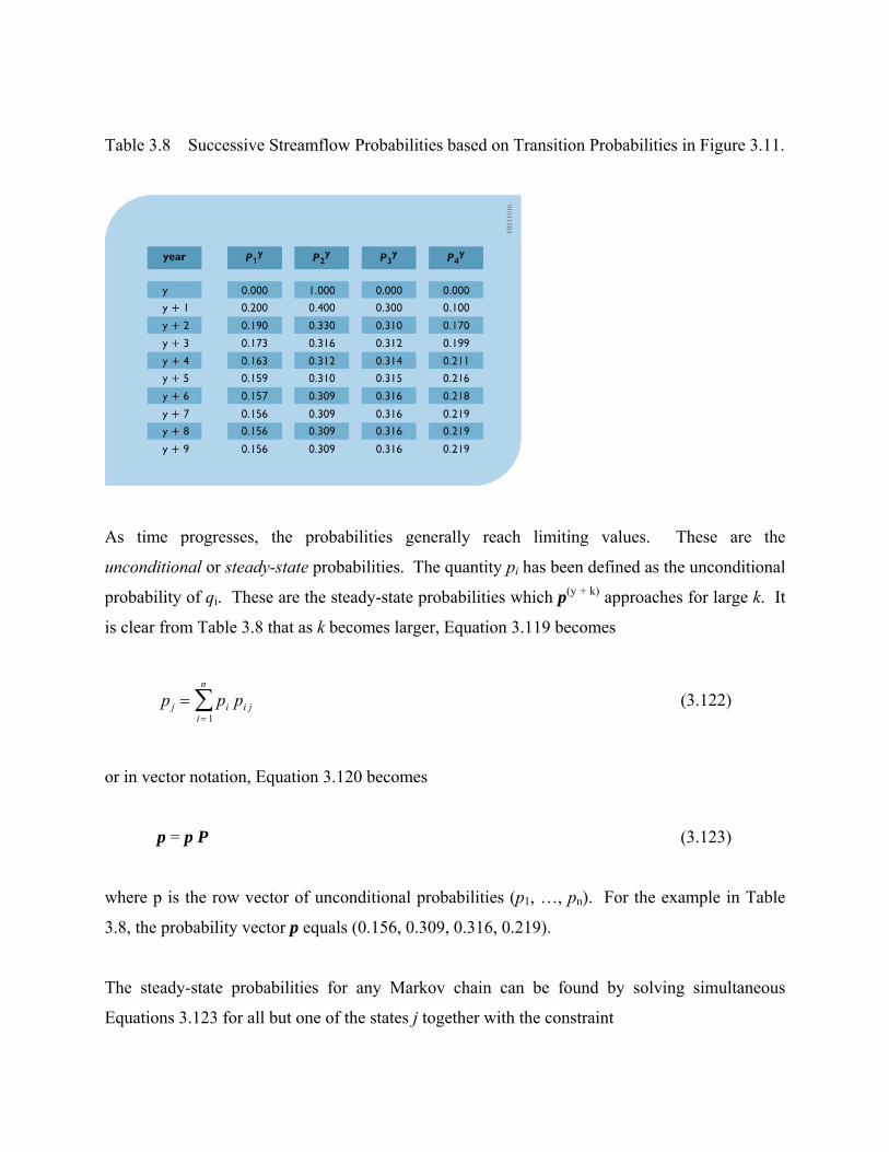
Table 3.8 Successive Streamflow Probabilities based on Transition Probabilities in Figure 3.11.

As time progresses, the probabilities generally reach limiting values. These are the

unconditional or steady-state probabilities. The quantity pi has been defined as the unconditional

probability of qi. These are the steady-state probabilities which p(y + k) approaches for large k. It

is clear from Table 3.8 that as k becomes larger, Equation 3.119 becomes

(3.122) pj = pi pi ji = 1

n

∑

or in vector notation, Equation 3.120 becomes

p = p P (3.123)

where p is the row vector of unconditional probabilities (p1, …, pn). For the example in Table

3.8, the probability vector p equals (0.156, 0.309, 0.316, 0.219).

The steady-state probabilities for any Markov chain can be found by solving simultaneous

Equations 3.123 for all but one of the states j together with the constraint

(3.124) 1

1n

ii

p=

=∑

Annual streamflows are seldom as highly correlated as the flows in this example. However,

monthly, weekly, and especially daily streamflows generally have high serial correlations.

Assuming that the unconditional steady-state probability distributions for monthly streamflows

are stationary, a Markov chain can be defined for each month’s steamflow. Since there are 12

months in a year, there would be 12 transition matrices, the elements of which could be denoted

as . Each defines the probability of a streamflow tijp 1t

jq + in month t + 1, given a streamflow

in month t. The steady-state stationary probability vectors for each month can be found by the

procedure outlined above, except that now all 12 matrices are used to calculate all 12 steady-state

probability vectors. However, once the steady-state vector p is found for one month, the others

are easily computed using Equation 3.121 with t replacing y.

tiq

7.3 Properties of time-series statistics

The statistics most frequently used to describe the distribution of a continuous-state stationary

stochastic process are the sample mean, variance, and various autocorrelations. Statistical

dependence among the observations, as is frequently the case in time series, can have a marked

effect on the distribution of these statistics. This part of Section 7 reviews the sampling

properties of these statistics when the observations are a realization of a stochastic process.

The sample mean

X =1n

Xii=1

n

∑ (3.125)

when viewed as a random variable is an unbiased estimate of the mean of the process µX,

because

[ ]1

1[ ]n

ii

E X E Xn =

= ∑ X= µ (3.126)

However, correlation among the Xi’s, so that ρX(k) ≠ 0 for k > 0, affects the variance of the

estimated mean .X

( ) ( ) ( )(22

1 1

1Varn n

X t Xt s

X E X E X Xn = =

)s X⎧ ⎫⎪ ⎪⎡ ⎤= − = − −⎨ ⎬⎢ ⎥⎣ ⎦ ⎪ ⎪⎩ ⎭∑∑µ µ µ

( )2 1

11 2 1

nX

Xk

k kn n

−

=

⎧ ⎫⎪ ⎛ ⎞= + −⎨ ⎜ ⎟⎝ ⎠⎪ ⎪⎩ ⎭

∑σ ρ ⎪⎬ (3.127)

The variance of X , equal to for independent observations, is inflated by the factor within

the brackets. For ρ

2 /X nσ

X(k) ≥ 0, as is often the case, this factor is a nondecreasing function of n, so

that the variance of X is inflated by a factor whose importance does not decrease with

increasing sample size. This is an important observation, because it means the average of a

correlated time series will be less precise than the average of a sequence of independent random

variables of the same length with the same variance.

A common model of stochastic series has

ρX(k) = [ρX(1)]k = ρk (3.128)

This correlation structure arises from the autoregressive Markov model discussed at length in

Section 8. For this correlation structure

Var X ( )=σ X

2

n1 +

2ρn

n 1− ρ( )− 1− ρn( )[ ]1 − ρ( )2

⎧ ⎨ ⎪

⎩ ⎪

⎫⎬⎪

⎭⎪ (3.129)

Substitution of the sample estimates for 2Xσ and ρX(1) in the equation above often yields a more

realistic estimate of the variance of X than does the estimate if the correlation structure

ρ

2 /Xs n

X(k) = ρk is reasonable; otherwise, Equation 3.127 may be employed. Table 3.9 illustrates the

affect of correlation among the Xt values on the standard error of their mean, equal to the square

root of the variance in Equation 3.127.

Table 3.9 Standard Error of X when σx = 0.25 and ρX(k) = ρk

The properties of the estimate of the variance of X,

ˆ σ X2 = vX

2 =1n

Xt − X (t =1

n

∑2

) (3.130)

are also affected by correlation among the Xt’s. Here v rather than s is used to denote the

variance estimator because n is employed in the denominator rather than n-1. The expected

value of 2xv becomes

( )1

2 2

1

1 21 1n

X X Xk

kE vn n n

−

=

⎧ ⎫⎪ ⎪⎛ ⎞⎡ ⎤ = − − −⎨ ⎬⎜ ⎟⎣ ⎦ ⎝ ⎠⎪ ⎪⎩ ⎭∑σ kρ (3.131)

The bias in 2Xv depends on terms involving ρX(1) through ρX(n − 1). Fortunately, the bias in

2Xv decreases with n and is generally unimportant when compared to its variance.

Correlation among the Xt’s also affects the variance of 2Xv . Assuming that X has a normal

distribution (here the variance of 2Xv depends on the fourth moment of X), the variance of 2

Xv

for large n is approximately (Kendall and Stuart, 1966, Sec 48.1).

Var vX2( )≅ 2

σ X4

n1 + 2 ρX

2 k( )k=1

∞

∑⎧ ⎨ ⎩

⎫ ⎬ ⎭

(3.132)

where for ρX(k) = ρk, Equation 3.132 becomes

Var vX2( )≅ 2

σ X4

n1 + ρ2

1− ρ2

⎛ ⎝ ⎜

⎞ ⎠ ⎟ (3.133)

Like the variance of X , the variance of 2Xv is inflated by a factor whose importance does not

decrease with n. This is illustrated by Table 3.10 which gives the standard deviation of 2Xv

divided by the true variance 2Xσ as a function of n and ρ when the observations have a normal

distribution and ρX(k) = ρk. This would be the coefficient of variation of 2Xv were it not biased.

A fundamental problem of time-series analyses is the estimation or description of the

relationship among the random variable values at different times. The statistics used to describe

this relationship are the autocorrelations. Several estimates of the autocorrelations have been

suggested. A simple and satisfactory estimate recommended by Jenkins and Watts (1968) is

( )( )( )

( )1

2

1

ˆ

n k

t t kt

X k n

tt

x x x xk r

x x

−

+=

=

− −= =

−

∑

∑ρ (3.134)

Table 3.10. Standard Deviation of ( 2 2/ )X Xv σ When Observations Have a Normal Distribution and ρX(k) = ρk

Here rk is the ratio of two sums where the numerator contains n − k terms and the denominator

contains n terms. The estimate rk is biased, but unbiased estimates frequently have larger mean

square errors (Jenkins and Watts, 1968). A comparison of the bias and variance of r1 is provided

by the case when the Xt’s are independent normal variates. Then (Kendall and Stuart, 1966)

[ ]11E rn

= − (3.135a)

and

Var r1( )=n − 2( )2

n2 n − 1( )≅1n

(3.135b)

For n = 25, the expected value of r1 is − 0.04 rather than the true value of zero; its standard

deviation is 0.19. This results in a mean square error of (E[r1])2 + Var(r1) = 0.0016 + 0.0353 =

0.0369. Clearly, the variance of r1 is the dominant term.

For Xt values that are not independent, exact expressions for the variance of rk generally are not

available. However, for normally distributed Xt and large n (Kendall and Stuart, 1966),

Var rk( )≅1n

ρx2 l( )[

l = −∞

+∞

∑ + ρx l + k( )ρx l − k( )

− 4ρx k( )ρx l( )ρx k − l( )+ 2ρx2 k( )ρx

2 l( )] (3.136)

If ρX(k) is essentially zero for k > q, then the simpler expression (Box et al., 1994)

Var rk( )≅1n

1 + 2 ρx2 l( )

t =1

q

∑⎡

⎣ ⎢

⎤

⎦ ⎥ (3.137)

is valid for rk corresponding to k > q. Thus for large n, Var(rk) ≥ l/n and values of rk will

frequently be outside the range of ± 1.65/ n , even though ρx(k) may be zero.

If ρX(k) = ρk, Equation 3.137 reduces to

Var rk( )≅1n

l + ρ2( ) l − ρ2k( )l − ρ2 − 2kρ2k

⎡

⎣ ⎢ ⎢

⎤

⎦ ⎥ ⎥ (3.138)

In particular for rl, this gives

Var r1( )≅1n

1− ρ2( ) (3.139)

Approximate values of the standard deviation of rl for different values of n and ρ are given in

Table 3.11.

The estimates of rk and rk+j are highly correlated for small j; this causes plots of rk versus k to

exhibit slowly varying cycles when the true values of ρX(k) may be zero. This increases the

difficulty of interpreting the sample autocorrelations.

Table 3.11. Approximate Standard Deviation of r1 When Observations Have a Normal Distribution and ρX(k) = ρk

8. Synthetic streamflow generation

8.1 Introduction

This section is concerned primarily with ways of generating sample data such as streamflows,

temperatures and rainfall that are used in water resource systems simulation studies (e.g. as

introduced in the next section). The models and techniques discussed in this section can be used

to generate any number of quantities used as inputs to simulation studies. For example Wilks

(1998, 2002) discusses the generation of wet and dry days, rainfall depths on wet days, and

associated daily temperatures. The discussion here is directed toward the generation of

streamflows because of the historic development and frequent use of these models in that context

(Matalas and Wallis, 1976). In addition, they are relatively simple compared to more complete

daily weather generators and many other applications. Generated streamflows have been called

synthetic to distinguish them from historical observations (Fiering, 1967). The activity has been

called stochastic hydrologic modeling. More detailed presentations can be found in Marco et al.

(1989) and Salas (1993).

River basin simulation studies can use many sets of streamflow, rainfall, evaporation, and/or

temperature sequences to evaluate the statistical properties of the performance of alternative

water resources systems. For this purpose, synthetic flows and other generated quantities should

resemble, statistically, those sequences that are likely to be experienced during the planning

period. Figure 3.12 illustrates how synthetic streamflow, rainfall, and other stochastic sequences

are used in conjunction with projections of future demands and other economic data to determine

how different system designs and operating policies might perform.

Figure 3.12. Structure of a simulation study, indicating the transformation of a synthetic

streamflow sequence, future demands and a system design and operating policy into system

performance statistics.

Use of only the historical flow or rainfall record in water resource studies does not allow for the

testing of alternative designs and policies against the range of sequences that are likely to occur

in the future. We can be very confident that the future historical sequence of flows will not be the

historical one, yet there is important information in that historical record. That information is not

fully used if only the historical sequence is simulated. By fitting continuous distributions to the

set of historical flows and then by using those distributions to generate other sequences of flows,

all of which are statistically similar and equally likely, gives one a broader range of inputs to

simulation models. Testing designs and policies against that broader range of flow sequences

that could occur more clearly identifies the variability and range of possible future performance

indicator values. This in turn should lead to the selection of more robust system designs and

policies.

The use of synthetic streamflows is particularly useful for water resource systems having large

amounts of over-year storage. Use of only the historical hydrologic record in system simulation

yields only one time history of how the system would operate from year to year. In water

resource systems having relatively little storage so that reservoirs and/or groundwater aquifers

refill almost every year, synthetic hydrologic sequences may not be needed if historical

sequences of a reasonable length are available. In this second case, a 25-year historic record

provides 25 descriptions of the possible within-year operation of the system. This may be

sufficient for many studies.

Generally, use of stochastic sequences is thought to improve the precision with which water

resource system performance indices can be estimated, and some studies have shown this to be

the case (Vogel and Shallcross, 1996; Vogel and Stedinger, 1988). In particular, if system

operation performance indices have thresholds and shape breaks, then the coarse descriptions

provided by historical series are likely to provide relative inaccurate estimates of the expected

values of such statistics. For example, suppose that shortages only invoke nonlinear penalties on

average one year in 20. Then in a 60-year simulation there is a 19% probability that the penalty

will be invoked at most once, and an 18% probability it will be invoked 5 or more times. Thus

the calculation of the annual average value of the penalty would be highly unreliable unless some

smoothing of the input distributions is allowed associated with a long simulation analysis.

On the other hand, if one is only interested in the mean flow, or average benefits that are mostly

a linear function of flows, then use of stochastic sequences will probably add little information to

what is obtained simply by simulating the historical record. After all, the fitted models are

ultimately based on the information provided in the historical record, and their use does not

produce new information about the hydrology of the basin.

If in a general sense one has available n years of record, the statistics of that record can be used

to build a stochastic model for generating thousands of years of flow. These synthetic data can

then be used to estimate more exactly the system performance, assuming, of course, that the

flow-generating model accurately represents nature. But the initial uncertainty in the model

parameters resulting from having only n years of record would still remain (Schaake and Vicens,

1980).

An alternative is to run the historical record (if it is sufficient complete at every site and contains

no gaps of missing data) through the simulation model to generate n years of output. That output

series can be processed to produce estimates of system performance. So the question is: is it

better to generate multiple input series based on uncertain parameter values and use those to

determine average system performance with great precision, or is it sufficient to just model the n-

year output series that results from simulation of the historical series?

The answer seems to depend upon how well behaved the input and output series are. If the

simulation model is linear, it does not make much difference. If the simulation model were

highly nonlinear, then modeling the input series would appear to be advisable. Or if one is

developing reservoir operating policies, there is a tendency to make a policy sufficiently complex

that it deals very well with the few droughts in the historical record but at the same time giving a

false sense of security and likely misrepresenting the probability of system performance failures.

Another situation where stochastic data generating models are useful is when one wants to

understand the impact on system performance estimates of the parameter uncertainty stemming

from short historical records. In that case, parameter uncertainty can be incorporated into

streamflow generating modes so that the generated sequences reflect both the variability that one

would expect in flows over time as well as the uncertainty of the parameter values of the models

that describe that variability (Valdes et al., 1977; Stedinger and Taylor, 1982; Stedinger, Pei and

Cohn, 1985; Vogel and Stedinger, 1988).

If one decides to use a stochastic data generator, the challenge is to use a model that

appropriately describes the important relationships, but does not attempt to reproduce more

relationships than are justified or that can be estimated with available data sets.

Two basic techniques are used for streamflow generation. If the streamflow population can be

described by a stationary stochastic process, a process whose parameters do not change over

time, and if a long historical streamflow record exists, then a stationary stochastic streamflow

model may be fit to the historical flows. This statistical model can then generate synthetic

sequences that describe selected characteristics of the historical flows. Several such models are

discussed below.

The assumption of stationarity is not always plausible, particularly in river basins that have

experienced marked changes in runoff characteristics due to changes in land cover, land use,

climate, or the utilization of groundwater during the period of flow record. Similarly, if the

physical characteristics of a basin will change substantially in the future, the historical

streamflow record may not provide reliable estimates of the distribution of future unregulated

flows. In the absence of the stationarity of streamflows or a representative historical record, an

alternative scheme is to assume that precipitation is a stationary stochastic process and to route

either historical or synthetic precipitation sequences through an appropriate rainfall-runoff model

of the river basin.

8.2 Streamflow generation models

The first step in the construction of a statistical streamflow generating model is to extract from

the historical streamflow record the fundamental information about the joint distribution of flows

at different sites and at different times. A streamflow model should ideally capture what is

judged to be the fundamental characteristics of the joint distribution of the flows. The

specification of what characteristics are fundamental is of primary importance.

One may want to model as closely as possible the true marginal distribution of seasonal flows

and/or the marginal distribution of annual flows. These describe both how much water may be

available at different times and also how variable is that water supply. Also, modeling the joint

distribution of flows at a single site in different months, seasons, and years may be appropriate.

The persistence of high flows and of low flows, often described by their correlation, affects the

reliability with which a reservoir of a given size can provide a given yield (Fiering, 1967;

Lettenmaier and Burges, 1977a,b; Thyer and Kuczera, 2000). For multi-component reservoir

systems, reproduction of the joint distribution of flows at different sites and at different times

will also be important.

Sometimes, a streamflow model is said to resemble statistically the historical flows if the

streamflow model produces flows with the same mean, variance, skew coefficient,

autocorrelations, and/or cross correlations as were observed in the historic series. This definition

of statistical resemblance is attractive because it is operational and requires that an analyst need

only find a model that can reproduce the observed statistics. The drawback of this approach is

that it shifts the modeling emphasis away from trying to find a good model of marginal

distributions of the observed flows and their joint distribution over time and over space, given

the available data, to just reproducing arbitrarily selected statistics. Defining statistical

resemblance in terms of moments may also be faulted for specifying that the parameters of the

fitted model should be determined using the observed sample moments, or their unbiased

counterparts. Other parameter estimation techniques, such as maximum likelihood estimators,

are often more efficient.

Definition of resemblance in terms of moments can also lead to confusion over whether the

population parameters should equal the sample moments, or whether the fitted model should

generate flow sequences whose sample moments equal the historical values. The two concepts

are different because of the biases (as discussed in Section 7) in many of the estimators of

variances and correlations (Matalas and Wallis, 1976; Stedinger, 1980, 1981; Stedinger and

Taylor, 1982a).

For any particular river basin study, one must determine what streamflow characteristics need to

be modeled. The decision should depend on what characteristics are important to the operation

of the system being studied, the available data, and how much time can be spared to build and

test a stochastic model. If time permits, it is good practice to see if the simulation results are in

fact sensitive to the generation model and its parameter values by using an alternative model and

set of parameter values. If the model’s results are sensitive to changes, then, as always, one must

exercise judgment in selecting the appropriate model and parameter values to use.

This section presents a range of statistical models for the generation of synthetic data. The

necessary sophistication of a data-generating model depends on the intended use of the data.

Section 8.3 below presents the simple autoregressive Markov model for generating annual flow

sequences. This model alone is too simple for many practical studies, but is useful for illustrating

the fundamentals of the more complex models that follow. It seems, therefore, worth some time

exploring the properties of this basic model.

Subsequent sections discuss how flows with any marginal distribution can be produced and

present models for generating sequences of flows that can reproduce the persistence of historical

flow sequences. Other parts of this section present models for generating concurrent flows at

several sites and for generating seasonal or monthly flows that preserve the characteristics of

annual flows. More detailed discussions for those wishing to study synthetic streamflow models

in greater depth can be found in Marco et al. (1989) and Salas (1993).

8.3 A simple autoregressive model

A simple model of annual streamflows is the autoregressive Markov model. The historical

annual flows qy are thought of as particular values of a stationary stochastic process Qy. The

generation of annual streamflows and other variables would be a simple matter if annual flows

were independently distributed. In general, this is not the case and a generating model for many

phenomena should capture the relationship between values in different years or in other different

time periods. A common and reasonable assumption is that annual flows are the result of a first-

order Markov process (as discussed in Section 7.2).

Assume for now that annual streamflows are normally distributed. In some areas, the

distribution of annual flows is in fact nearly normal. Streamflow models that produce nonnormal

streamflows are discussed as an extension of this simple model.

The joint normal density function of two streamflows Qy and Qw in years y and w having mean

µ, variance σ2, and year-to-year correlation ρ between flows is

( )( )0.52 2

1,2 1

y wf q qπσ ρ

=−

( ) ( )( ) ( )( )

2 2

2 2

2exp

2 1y y w wq q q q⎡ ⎤− µ − ρ − µ − µ + − µ

⎢ ⎥⋅⎢ ⎥σ − ρ⎣ ⎦

(3.140)

The joint normal distribution for two random variables with the same mean and variance depend

only on their common mean µ, variance σ2, and the correlation ρ between the two (or

equivalently the covariance ρσ2).

The sequential generation of synthetic streamflows requires the conditional distribution of the

flow in one year given the value of the flows in previous years. However, if the streamflows are

a first-order (lag 1) Markov process, then the dependence of the distribution of the flow in year y

+ 1 on flows in previous years depends entirely on the value of the flow in year y. In addition, if

the annual streamflows have a multivariate normal distribution, then the conditional distribution

of Qy+1 is normal with mean and variance

E[Qy+1⏐Qy = qy] = µ + ρ(qy − µ)

(3.141)

Var(Qy+1⏐Qy = qy) = σ2(1 − ρ2)

where qy is the value of the random variable Qy in year y. Notice that the larger the absolute

value of the correlation ρ between the flows, the smaller the conditional variance of Qy+1, which

in this case does not depend at all on the value qy.

Synthetic normally distributed streamflows that have mean µ, variance σ2, and year-to-year

correlation ρ, are produced by the model

Qy+1 = µ + ρ(Qy − µ) + Vyσ 21 ρ− (3.142)

where Vy is a standard normal random variable, meaning that it has zero mean, E[Vy] = 0, and

unit variance, . The random variable V2yE V 1⎡ ⎤ =⎣ ⎦ y is added here to provide the variability in

Qy+1 that remains even after Qy is known. By construction, each Vy is independent of past flows

Qw where w ≤ y, and Vy is independent of Vw for w ≠ y. These restrictions imply that

E[VwVy] = 0 w ≠ y (3.143)

and

E[(Qw − µ)Vy] = 0 w ≤ y (3.144)

Clearly, Qy+1 will be normally distributed if both Qy and Vy are normally distributed because

sums of independent normally distributed random variables are normally distributed.

It is a straightforward procedure to show that this basic model indeed produces streamflows with

the specified moments, as demonstrated below.

Using the fact that E[Vy] = 0, the conditional mean of Qy+1 given that Qy equals qy is

E[Qy+1|qy] = E[µ + ρ(qy − µ) + Vy σ 21 ρ− ] = µ + ρ(qy − µ) (3.145)

Since E{ Vy2 ] = Var[Vy] = 1, the conditional variance of Qy+1 is

Var[Qy+1⏐qy] = E[{Qy+1 − E[Qy+1⏐qy]}2⏐qy]

= E[ { µ + ρ(qy − µ) + Vy σ 21 ρ− − [µ + ρ(qy − µ)] }2

= E[Vy σ 21 ρ− ]2 = σ2(1 − ρ2) ] (3.146)

Thus this model produces flows with the correct conditional mean and variance.

To compute the unconditional mean of Qy+1 one first takes the expectation of both sides of

Equation 3.142 to obtain

E[Qy+1] = µ + ρ (E[Qy] − µ) + E[Vy] σ 21 ρ− (3.147)

where E[Vy] = 0. If the distribution of streamflows is independent of time so that for all y,

E[Qy+1] = E[Qy] = E[Q], it is clear that (1 − ρ) E[Q] = (1 − ρ) µ or

E[Q] = µ (3.148)

Alternatively, if Qy for y = 1 has mean µ, then Equation 3.147 indicates that Q2 will have mean

µ. Thus repeated application of the Equation 3.147 would demonstrate that all Qy for y > 1 have

mean µ.

The unconditional variance of the annual flows can be derived by squaring both sides of 3.142 to

obtain

E[(Qy+1 − µ)2] = E[{ρ(Qy − µ) + Vyσ 2 21 }ρ− ]

= ρ2E[(Qy − µ)2] + 2ρσ 21 ρ− E[(Qy − µ)Vy] + σ2(1 − ρ2)E (3.149) 2yV⎡ ⎤⎣ ⎦

Because Vy is independent of Qy (Equation 3.144), the second term on the right-hand side of

Equation 3.149 vanishes. Hence the unconditional variance of Q satisfies

E[(Qy+1 − µ)2] = ρ2 E [(Qy − µ)2] + σ2 (1 − ρ2) (3.150)

Assuming that Qy+1 and Qy have the same variance yields

E[(Q − µ)2] = σ2 (3.151)

so that the unconditional variance is σ2, as required.

Again, if one does not want to assume that Qy+1 and Qy have the same variance, a recursive

argument can be adopted to demonstrate that if Q1 has variance σ2, then Qy for y ≥ 1 has variance

σ2.

The covariance of consecutive flows is another important issue. After all the whole idea of

building these time series models is to describe the year-to-year correlation of the flows. Using

Equation 3.142 one can show that the covariance of consecutive flows must be

E[ (Qy+1 − µ)(Qy − µ) ] = E{[ρ(Qy − µ) + Vy σ 21 ρ− ](Qy − µ)}

= ρ E[(Qy − µ)2] = ρ σ2 (3.152)

where E[(Qy − µ)Vy] = 0 because Vy and Qy are independent (Equation 3.144).

Over a longer time scale, another property of this model is that the covariance of flows in year y

and y + k is

E[(Qy+k − µ) (Qy − µ)] = ρkσ2 (3.153)

This equality can be proven by induction. It has already been shown for k = 0 and 1. If it is true

for k = j − 1, then

E[(Qy+j − µ) (Qy − µ)] = E{[ρ(Qy+j−1 − µ) + Vy+j−1σ 21 ρ− ] (Qy − µ)}

= ρ E[ (Qy − µ)] (Qy+j−1 − µ)] = ρ[ρj−1σ2] = ρjσ2

= ρ[ρj−1σ2] = ρjσ2 (3.154)

where E[(Qy − µ)Vy+j−1] = 0 for j ≥ 1. Hence Equation 3.153 is true for any value of k.

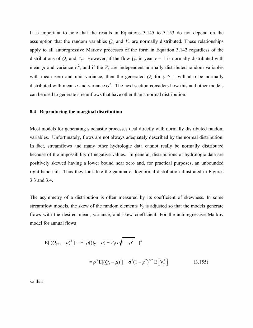
It is important to note that the results in Equations 3.145 to 3.153 do not depend on the

assumption that the random variables Qy and Vy are normally distributed. These relationships

apply to all autoregressive Markov processes of the form in Equation 3.142 regardless of the

distributions of Qy and Vy. However, if the flow Qy in year y = 1 is normally distributed with

mean µ and variance σ2, and if the Vy are independent normally distributed random variables

with mean zero and unit variance, then the generated Qy for y ≥ 1 will also be normally

distributed with mean µ and variance σ2. The next section considers how this and other models

can be used to generate streamflows that have other than a normal distribution.

8.4 Reproducing the marginal distribution

Most models for generating stochastic processes deal directly with normally distributed random

variables. Unfortunately, flows are not always adequately described by the normal distribution.

In fact, streamflows and many other hydrologic data cannot really be normally distributed

because of the impossibility of negative values. In general, distributions of hydrologic data are

positively skewed having a lower bound near zero and, for practical purposes, an unbounded

right-hand tail. Thus they look like the gamma or lognormal distribution illustrated in Figures

3.3 and 3.4.

The asymmetry of a distribution is often measured by its coefficient of skewness. In some

streamflow models, the skew of the random elements Vy is adjusted so that the models generate

flows with the desired mean, variance, and skew coefficient. For the autoregressive Markov

model for annual flows

E[ (Qy+1 − µ)3 ] = E [ρ(Qy − µ) + Vyσ 1 − ρ2 ]3

= ρ3 E[(Qy − µ)3] + σ3(1 − ρ2)3/2 E 3yV⎡ ⎤⎣ ⎦ (3.155)

so that

3 2

Q 3 3

E[( ) ] (1 )1

Q − −= =

−µ ργ

σ ρ

3/ 2

(3.156)

By appropriate choice of the skew of Vy, the desired skew coefficient of the annual flows can be

produced. This method has often been used to generate flows that have approximately a gamma

distribution by using Vy’s with a gamma distribution and the required skew. The resulting

approximation is not always adequate (Lettenmaier and Burges, 1977a).

The alternative and generally preferred method is to generate normal random variables and then

transform these variates to streamflows with the desired marginal distribution. Common choices

for the distribution of streamflows are the two-parameter and three-parameter lognormal

distributions or a gamma distribution. If Qy is a lognormally distributed random variable, then

Qy = τ + exp (Xy) (3.157)

where Xy is a normal random variable. When the lower bound τ is zero, Qy has a two-parameter

lognormal distribution. Equation 3.157 transforms the normal variates Xy into lognormally

distributed streamflows. The transformation is easily inverted to obtain

Xy = ln(Qy − τ) for Qy > τ (3.158)

where Qy must be greater than its lower bound τ.

The mean, variance, skewness of Xy and Qy are related by the formulas (Matalas, 1967)

µQ = τ + exp (µX + 2X

12

σ )

2Qσ = exp (2µX + 2

Xσ ) [exp ( )2Xσ − 1] (3.159)

γQ = exp (3σ X

2 ) − 3 exp (σ X2 ) + 2

[exp (σ X2 ) − 1]3/2

If normal variates Xys and Xy

u are used to generate lognormally distributed streamflows

Qys and Qy

u at sites s and u, then the lag-k correlation of the Qy’s, denoted ρQ(k; s, u), is

determined by the lag-k correlation of the X variables, denoted ρX(k; s, u), and their variances

and , where 2X (s)σ 2

X (u)σ

{ } { }

X X XQ 1/ 2 1/ 22 2

X X

exp [ (k; s, u) (s) (u)] 1(k;s, u)exp [ (s)] 1 exp [ (u)] 1

ρ σ σρσ σ

−=

− − (3.160)

The correlations of the can be adjusted, at least in theory, to produce the observed

correlations among the variates. However, more efficient estimates of the true correlation of

the values are generally obtained by transforming the historical flows into their normal

equivalent

syX

syQ

syQ s

yq

s sy yx n(q )τ= −l and using the historical correlations of these values as estimators

of ρ

syx

X(k; s, u) (Stedinger, 1981).

Some insight into the effect of this logarithmic transformation can be gained by considering the

resulting model for annual flows at a single site. If the normal variates follow the simple

autoregressive Markov model

Xy+1 − µ = ρX (Xy − µ) + Vy σX2X1 ρ− (3.161)

then the corresponding Qy follow the model (Matalas, 1967)

Qy+1 = τ + Dy { exp[µx(1 − ρx)]}(Qy − τ)ρX (3.162)

where

Dy = exp [ (1 − 2Xρ )1/2 σX Vy] (3.163)

The conditional mean and standard deviation of Qy+1 given that Qy = qy now depends on (qy −

τ)ρX . Because the conditional mean of Qy+1 is no longer a linear function of qy, the streamflows

are said to exhibit differential persistence: low flows are now more likely to follow low flows

than high flows and high flows are more likely to follow high flows than low flows. This is a

property often attributed to real streamflow distributions. Models can be constructed to capture

the relative persistence of wet and dry periods (Matalas and Wallis, 1976; Salas, 1993; Thyer and

Kuczera, 2000). Many weather generators for precipitation and temperature include such

tendencies by employing a Markov chain description of the occurrence of wet and dry days

(Wilks, 1998).

8.5 Multivariate models

If long concurrent streamflow records can be constructed at the several sites at which synthetic

streamflows are desired, then ideally a general multi-site streamflow model could be employed.

O’Connell (1977), Ledolter (1978), Salas et al. (1980) and Salas (1993) discuss multivariate

models and parameter estimation. Unfortunately, model identification (parameter value

estimation) is very difficult for the general multivariate models.

This section illustrates how the basic univariate annual-flow model in Section 8.3 can be

generalized to the multivariate case. This exercise reveals how multivariate models can be

constructed to reproduce specified variances and covariances of the flow vectors of interest, or

some transformation of those values. This multi-site generalization of the annual AR(1) or

autoregressive Markov model follows the approach taken by Matalas and Wallis (1976). This

general approach can be further extended to generate multi-site/multi-season modeling

procedures, as is done in Section 8.6 employing what have been called disaggregation models.

However, while the size of the model matrices and vectors increases, the model is fundamentally

the same from a mathematical viewpoint. Hence this section starts with the simpler case of an

annual flow model.

For simplicity of presentation and clarity, vector notation is employed. Let Zy = ( 1yZ , . . . ,

nyZ )T be the column vector of transformed zero-mean annual flows at sites s = 1, 2, . . . , n, so

that

(3.164) syE[Z ] 0=

In addition, let Vy = ( )T1 ny y, . . . ,V V be a column vector of standard-normal random variables,

where is independent of for (r, w) ≠ (s, y) and independent of past flows syV r

wV rwZ where y ≥

w. The assumption that the variables have zero mean implicitly suggests that the mean value has

already been subtracted from all the variables. This makes the notation simpler and eliminates

the need to include a constant term in the models. With all the random variables having zero

mean, one can focus on reproducing the variances and covariances of the vectors included in a

model.

A sequence of synthetic flows can be generated by the model

Zy+1 = AZy + BVy (3.165)

where A and B are (n × n) matrices whose elements are chosen to reproduce the lag 0 and lag 1

cross covariances of the flows at each site. The lag 0 and lag 1 covariances and cross covariances

can most economically be manipulated by use of the two matrices S0 and S1. The lag-zero

covariance matrix, denoted S0, is defined as

S0 = E[ZyTyZ ] (3.166)

and has elements

S0(i, j) = E (3.167) i j⎡⎣ y yZ Z ⎤⎦

The lag-one covariance matrix, denoted S1, is defined as

S1 = E[Zy+1TyZ ] (3.168)

and has elements

S1(i, j) = E (3.169) i j1+⎡ ⎤⎣ ⎦y yZ Z

The covariances do not depend on y because the streamflows are assumed to be stationary.

Matrix S1 contains the lag 1 covariances and lag 1 cross covariances. S0 is symmetric because

the cross covariance S0(i, j) equals S0(j, i). In general, S1 is not symmetric.

The variance-covariance equations that define the values of A and B in terms of S0 and S1 are

obtained by manipulations of Equation 3.165. Multiplying both sides of that equation by ZyT and

taking expectations yields

T T

1E E Ey y y y y y+⎡ ⎤ ⎡ ⎤ ⎡= +⎣ ⎦ ⎣ ⎦ ⎣Z Z AZ Z BV ZT ⎤⎦ (3.170)

The second term on the right-hand side vanishes because the components of Zy and Vy are

independent. Now the first term in Equation 3.170, E[AZy ZyT], is a matrix whose (i, j)th

element equals

= (3.171) E aik Z y

kZ yi

k =1

n

∑⎡

⎣ ⎢

⎤

⎦ ⎥

n

k 1

E[ ]k iik y ya Z Z

=∑

The matrix with these elements is the same as the matrix AE T⎡ ⎤⎣ ⎦y yZ Z .

Hence, A – the matrix of constants – can be pulled through the expectation operator just as is

done in the scalar case where E[aZy + b] = aE[Zy] + b for fixed constants a and b.

Substituting S0 and S1 for the appropriate expectations in Equation 3.170 yields

S1 = ASo or A = S1S0-1 (3.172)

A relationship to determine the matrix B is obtained by multiplying both sides of Equation 3.165

by its own transpose (this is equivalent to squaring both sides of the scalar equation a = b) and

taking expectations to obtain

E[Zy+1T

1y+Z ] = E[AZyTyZ AT] + E[AZy

TyV BT]

+ E[BVyZyAT] + E[BVyTyV BT] (3.173)

The second and third terms on the right-hand side of Equation 3.173 vanish because the

components of Zy and Vy are independent and have zero mean. E Ty y⎡ ⎤⎣ ⎦V V equals the identity

matrix because the components of Vy are independently distributed with unit variance. Thus

S0 = ASoAT + BBT (3.174)

Solving of the B matrix one finds that it should satisfy

BBT = S0 − ASoAT = S0 − S1 S0-1S0

T (3.175)

The last equation results from substitution of the relationship for A given in Equation 3.172 and

the fact that S0 is symmetric; hence S0-1 is symmetric.

It should not be too surprising that the elements of B are not uniquely determined by Equation

3.175. The components of the random vector Vt may be combined in many ways to produce the

desired covariances as long as B satisfies Equation 3.175. A lower triangular matrix that

satisfies Equation 3.175 can be calculated by Cholesky decomposition (Young, 1968; Press et

al., 1986).

Matalas and Wallis (1976) call Equation 3.165 the lag-1 model. They did not call it the Markov

model because the streamflows at individual sites do not have the covariances of an

autoregressive Markov process given in Equation 3.153. They suggest an alternative model for

what they call the Markov model. It has the same structure as the lag-1 model except it does not

preserve the lag-1 cross-covariances. By relaxing this requirement, they obtain a simpler model

with fewer parameters that generates flows having covariances of an autoregressive Markov

process at each site. In their Markov model, the new A matrix is simply a diagonal matrix whose

diagonal elements are the lag-1 correlations of flows at each site:

A = diag[ ρ(1; i, i,) ] (3.176)

where ρ(1; i, i) is the lag-one correlation of flows at site i.

The corresponding B matrix depends on the new A matrix and S0, where as before

BBT = S0 − AS0AT (3.177)

The idea of fitting time series models to each site separately and then correlating in innovations

in those separate models to reproduce the cross-correlation between the series is a very general

and useful modeling idea that has seen a number of applications with different time series

models (Matalas and Wallis, 1976; Stedinger et al., 1985; Camacho et al., 1985; Salas, 1993).

8.6 Multi-season, multi-site models

In most studies of surface water systems it is necessary to consider the variations of flows within

each year. Streamflows in most areas have within-year variations, exhibiting wet and dry

periods. Similarly, water demands for irrigation, municipal, and industrial uses also vary, and

the variations in demand are generally out of phase with the variation in within-year flows; more

water is usually desired when streamflows are low and less is desired when flows are high. This

increases the stress on water delivery systems and makes it all the more important that time

series models of streamflows, precipitation and other hydrological variables correctly reproduce

the seasonality of hydrological processes.

This section discusses two approaches to generating within-year flows. The first approach is

based on the disaggregation of annual flows produced by an annual flow generator to seasonal

flows. Thus the method allows for reproduction of both the annual and seasonal characteristics of

streamflow series. The second approach generates seasonal flows in a sequential manner, as was

done for the generation of annual flows. Thus the models are a direct generalization of the

annual flow models already discussed.

8.6.1 Disaggregation model

The disaggregation model proposed by Valencia and Schaake (1973) and extended by Mejia and

Rousselle (1976) and Tao and Delleur (1976) allows for the generation of synthetic flows that

reproduce statistics both at the annual level and at the seasonal level. Subsequent improvements

and variations are described by Stedinger and Vogel (1984), Maheepala and Perera (1996),

Koutsoyiannis and Manetas (1996) and Tarboton et al. (1998).

Disaggregation models can be used for either multiseason single-site or multisite streamflow

generation. They represent a very flexible modeling framework for dealing with different time

or spatial scales. Annual flows for the several sites in question or the aggregate total annual flow

at several sites can be the input to the model (Grygier and Stedinger, 1988). These must be

generated by another model, such as those discussed in the previous sections. These annual

flows or aggregated annual flows are then disaggregated to seasonal values.

Let Zy = ( )T1 NZ ,..., Zy y be the column vector of N transformed normally distributed annual or

aggregate annual flows for N separate sites or basins. Next let Xy =

X1, y1 , ...,XT , y,

1 X1, y2 ,..., XTy

2 , ...,X1yn ,..., XTy

n( )Tbe the column vector of nT transformed normally

distributed seasonal flows for season t, year y, and site s. sXty

Assuming that the annual and seasonal series, , have zero mean (after the appropriate

transformation), the basic disaggregation model is

syZ and Xs

ty

Xy = AZy + BVy (3.178)

where Vy is a vector of nT independent standard normal random variables, and A and B are,

respectively, nT × N and nT × nT matrices. One selects values of the elements of A and B to

reproduce the observed correlations among the elements of Xy and between the elements of Xy

and Zy. Alternatively, one could attempt to reproduce the observed correlations of the

untransformed flows as opposed to the transformed flows, although this is not always possible

(Hoshi et al., 1978) and often produces poorer estimates of the actual correlations of the flows

(Stedinger, 1981).

The values of A and B are determined using the matrices Szz = E ⎡ ⎤⎣ ⎦T

y yZ Z , Szz = E , ST⎡⎣ y yZ Z ⎤⎦

⎤⎦ ⎤⎦

xx =

E , STy y⎡⎣X X xz = E , and ST⎡⎣ y yX Z zy = E T⎡ ⎤⎣ ⎦y yZ X where Szz was called S0 earlier. Clearly,

. If STxz zx=S S xz is to be reproduced, then by multiplying Equation 3.178 on the right by and

taking expectations, one sees that A must satisfy

TyZ

E (3.179) T E⎡ ⎤ ⎡=⎣ ⎦ ⎣y y y yX Z AZ ZT ⎤⎦

or

Sxz = ASzz (3.180)

Solving for the coefficient matrix A one obtains

A = Sxz1−

zzS (3.181)

To obtain an equation that determines the required values in matrix B, one can multiply both

sides of Equation 3.178 by their transpose and take expectations to obtain

Sxx = ASzzAT + BBT (3.182)

Thus to reproduce the covariance matrix Sxx, the B matrix must satisfy

BBT = Sxx − ASzzAT (3.183)

Equations 3.181 and 3.183 for determining A and B are completely analogous to Equations

3.172 and 3.175 for the A and B matrices of the lag 1 models developed earlier. However, for

the disaggregation model as formulated, BBT and hence the matrix B can actually be singular or

nearly so (Valencia and Schaake, 1973). This occurs because the real seasonal flows sum to the

observed annual flows. Thus given the annual flow at a site and all but one (T − 1) of the

seasonal flows, the value of the unspecified seasonal flow can be determined by subtraction.

If the seasonal variables styX correspond to nonlinear transformations of the actual flows s

tyQ ,

then BBT is generally sufficiently non-singular that a B matrix can be obtained by Cholesky

decomposition. On the other hand, when the model is used to generate values of styX to be

transformed into synthetic flows styQ , the constraint that these seasonal flows should sum to the

given value of the annual flow is lost. Thus the generated annual flows (equal to the sums of the

seasonal flows) will deviate from the values that were to have been the annual flows. Some

distortion of the specified distribution of the annual flows results. This small distortion can be

ignored, or each year’s seasonal flows can be scaled so that their sum equals the specified value

of the annual flow (Grygier and Stedinger, 1988). The latter approach eliminates the distortion

in the distribution of the generated annual flows by distorting the distribution of the generated

seasonal flows. Koutsoyiannis and Manetas (1996) improve upon the simple scaling algorithm

by including a step that rejects candidate vectors Xy if the required adjustment is too large and

instead generates another vector Xy. This reduces the distortion in the monthly flows that results

from the adjustment step.

The disaggregation model has substantial data requirements. When the dimension of Zy is n and

the dimension of the generated vector Xy is m, the A matrix has mn elements. The lower diagonal

B matrix and the symmetric Sxx matrix, upon which it depends, each have m(m + 1)/2 nonzero or

nonredundant elements. For example, when disaggregating two aggregate annual flow series to

monthly flows at five sites, n = 2 and m = 12 × 5 = 60 so that A has 120 elements while B and

Sxx each have 1830 nonzero or nonredundant parameters. As the number of sites included in the

disaggregation increases, the size of Sxx and B increases rapidly. Very quickly the model can

become over parameterized, and there will be insufficient data to estimate all parameters

(Grygier and Stedinger, 1988).

In particular, one can think of Equation 3.178 as a series of linear models generating each

monthly flow for k = 1, t = 1, …, 12; k = 2, t = 1, …, 12 up to k = n, t = 1, …, 12 that

reproduces the correlation of each with all n annual flows, , and all previously generated

monthly flows. Then when one gets to the last flow in the last month, the model will be

attempting to reproduce n + (12n − 1) = 13n − 1 annual to monthly and cross-correlations.

Because the model implicitly includes a constant, this means one needs k* = 13n years of data to

obtain a unique solution for this critical equation. For n = 3, k* = 39. One could say that with a

record length of 40 years, there would be only 1 degree of freedom left in the residual model

error variance described by B. That would be unsatisfactory.

ktyX

ktyX k

yZ

When flows at many sites or in many seasons are required, the size of the disaggregation model

can be reduced by disaggregation of the flows in stages. Such condensed models do not

explicitly reproduce every season-to-season correlation (Lane, 1979; Stedinger and Vogel, 1984;

Gryier and Stedinger, 1988; Koutsoyiannis and Manetas, 1996). Nor do they attempt to

reproduce the cross correlations among all the flow variates at the same site within a year (Lane,

1979; Stedinger et al., 1985). Contemporaneous models, like the Markov model developed

earlier in Section 8.5, are models developed for individual sites whose innovation vectors Vy

have the needed cross-correlations to reproduce the cross-correlations of the concurrent flows

(Camacho et al., 1985), as was done in Equation 3.177. Grygier and Stedinger (1991) describe

how this can be done for a condensed disaggregation model without generating inconsistencies.

8.6.2 Aggregation models

One can start with annual or seasonal flows, and break them down into flows in shorter periods

representing months or weeks. Alternatively one can start with a model that describes the

shortest time step flows. This latter approach has been referred to as aggregation to distinguish it

from disaggregation.

One method for generating multiseason flow sequences is to convert the time series of seasonal

flows Qty into a homogeneous sequence of normally distributed zero-mean unit-variance random

variables Zty. These can then be modeled by an extension of the annual flow generators that have

already been discussed. This transformation can be accomplished by fitting a reasonable

marginal distribution to the flows in each season so as to be able to convert the observed flows styq into their transformed counterparts s

tyz , and vice versa. Particularly, when shorter streamflow

records are available, these simple approaches may yield a reasonable model of some streams for

some studies. However, it implicitly assumes that the standardized series is stationary in the

sense that the season-to-season correlations of the flows do not depend on the seasons in

question. This assumption seems highly questionable.

This theoretical difficulty with the standardized series can be overcome by introducing a separate

streamflow model for each month. For example, the classic Thomas-Fiering model (Thomas and

Fiering, 1970) of monthly flows may be written

21, 1β β+ = + −t y t ty t tyZ Z V (3.184)

where the Zty’s are standard normal random variables corresponding to the streamflow in season

t of year y, βt is the season-to-season correlation of the standardized flows, and Vty are

independent standard normal random variables. The problem with this model is that it often fails

to reproduce the correlation among months during a year and thus misrepresents the risk of

multi-month and multi-year droughts (Hoshi et al., 1978).

For an aggregation approach to be attractive it is necessary to use a model with greater

persisitence than the Thomas-Fiering model. A general class of time series models that allow

reproduction of different correlation structures are the Box-Jenkins Autoregressive-Moving

average models (Box et al., 1994). These models are presented by the notation ARMA(p,q) for a

model which depends on p previous flows, and q extra innovations Vty. For example, Equation

3.142 would be called an AR(1) or AR(1,0) model. A simple ARMA(1,1) model is

Zt +1 = φ1 ⋅ Zt +Vt +1 −θ1 ⋅Vt (3.185)

The correlations of this model have the values

ρ1 = (1 - θ1 φ1 )(φ1− θ1)/(1 +θ12 − 2φ1 θ1) (3.186)

for the first lag. For i > 1

ρi = φ i−1ρ1 (3.187)

For φ values near one and 0 < θ1 < φ1 the autocorrelations ρk can decay much slower than

those of the standard AR(1) model.

The correlation function ρk of general ARMA(p,q) model

Zt +1 =i=1

p

∑ φi ⋅ Zt +1−i +Vt +1 −j =1

q

∑ θ j ⋅Vt +1− j (3.188)

is a complex function that must satisfy a number of conditions to ensure the resultant model is

stationary and invertible (Box et al., 1994)

ARMA(p,q) models have been extended to describe seasonal flow series by having their

coefficients depend upon the season – these are called periodic Autoregressive-Moving average

models, or PARMA. Salas and Obeysekera (1992), Salas and Fernandez (1993), and Claps et al.

(1993) discuss the conceptual basis of such stochastic streamflow models. For example, Salas

and Obeysekera (1992) found that low-order PARMA models, such as a PARMA(2,1), arise

from reasonable conceptual representations of persistence in rainfall, runoff, and groundwater

recharge and release. Claps et al. (1993, p. 2553) observe that the PARMA(2,2) model which

may be needed if one wants to preserve year-to-year correlation poses a parameter estimation

challenge that is almost unmanageable (see also Rasmussen et al., 1996). The PARMA (1,1)

model is more practical and easy to extend to the multivariate case (Hirsch, 1979; Stedinger et al.

1985; Salas, 1993; Rasmussen et al., 1996). Experience has shown that PARMA(1,1) models do

a better job of reproducing the correlation of seasonal flows beyond lag one (see for example,

Bartolini and Salas, 1993).

9. Stochastic simulation This section introduces stochastic simulation. Much more detail on simulation is contained in

later chapters. Simulation is the most flexible and widely used tool for the analysis of complex

water resources systems. Simulation is trial and error. One must define the system being

simulated, both its design and operating policy, and then simulate it to see how it works. If the

purpose is to find the best design and policy, many such alternatives must be simulated and their

results must be compared. When the number of alternatives to simulate becomes too large for

the time and money available for such analyses, some kind of preliminary screening, perhaps

using optimization models, may be justified. This use of optimization for preliminary screening

– i.e., for eliminating alternatives prior to a more detailed simulation – is also discussed in later

chapters.

As with optimization models, simulation models may be deterministic or stochastic. One of the

most useful tools in water resource systems planning is stochastic simulation. While

optimization can be used to help define reasonable design and operating policy alternatives to be

simulated, it takes those simulations to obtain the best insights of just how each such alternative

will perform. Stochastic simulation of complex water resources systems on digital computers

provides planners with a way to define the probability distributions of multiple performance

indices of those systems.

When simulating any system, the modeler designs an experiment. Initial flow, storage, and

water quality conditions must be specified if these are being simulated. For example, reservoirs

can start full, empty, or at random representative conditions. The modeler also determines what

data are to be collected on system performance and operation and how they are to be

summarized. The length of time the simulation is to be run must be specified and, in the case of

stochastic simulations, the number of runs to be made must also be determined. These

considerations are discussed in more detail by Fishman (2001) and in other books on simulation.

The use of stochastic simulation and the analysis of the output of such models are merely

introduced here primarily in the context of an example to illustrate what goes into a simulation

model and how one can deal with the information that is generated.

9.1 Generating random variables

Included in any stochastic simulation model is some provision for the generation of sequences of

random numbers that represent particular values of events such as rainfall, streamflows, or

floods. To generate a sequence of values for a random variable, the probability distribution for

the random variable must be specified. Historical data and an understanding of the physical

processes are used to select appropriate distributions and to estimate their parameters (as

discussed in Section 3.2).

Most computers have algorithms for generating random numbers uniformly distributed (equally

likely) between zero and one. This uniform distribution is defined by its cdf and pdf;

Fu(u) = 0 for u ≤ 0, u for 0 ≤ u ≤ 1 and 1 if u ≥1 (3.189)

and

fU(u) = 1 if 0 ≤ u ≤ 1 and 0 otherwise (3.190)

These uniform random variables can then be transformed into random variables with any desired

distribution. If FQ(qt) is the cumulative distribution function of a random variable Qt in period t,

then Qt can be generated using the inverse of the distribution.

Qt = FQ

-1[Ut] (3.191) Here Ut is the uniform random number used to generate Qt. This is illustrated in Figure 3.13.

Figure 3.13. The probability distribution of a random variable can be inverted to produce values

of the random variable.

Analytical expressions for the inverse of many distributions, such as the normal distribution, are

not known, so that special algorithms are employed to efficiently generate deviates with these

distributions (Fishman, 2001).

9.2 River basin simulation.

An example will demonstrate the use of stochastic simulation in the design and analysis of water

resource systems. Assume that farmers in a particular valley have been plagued by frequent

shortages of irrigation water. They currently draw water from an unregulated river to which they

have water rights. A government agency has proposed construction of a moderate-size dam on

the river upstream from points where the farmers withdraw water. The dam would be used to

increase the quantity and reliability of irrigation water available to the farmers during the

summer growing season.

After preliminary planning, a reservoir with an active capacity of 4 x 107 m3 has been proposed

for a natural dam site. It is anticipated that because of the increased reliability and availability of

irrigation water, the quantity of water desired will grow from an initial level of 3 x 107 m3/yr

after construction of the dam to 4 x 107 m3/yr within 6 years. After that, demand will grow more

slowly to 4.5 x 107 m3/yr, the estimated maximum reliable yield. The projected demand for

summer irrigation water is shown in Table 3.12.

A simulation study will evaluate how the system can be expected to perform over a 20-year

planning period. Table 3.13 contains statistics that describe the hydrology at the dam site. The

estimated moments are computed from the 45-year historic record.

Table 3.12. Projected Water Demand for Irrigation Water

Table 3.13. Characteristics of the River Flow

Using the techniques discussed in the previous section, a Thomas-Fiering model is used to

generate 25 lognormally distributed synthetic streamflow sequences. The statistical

characteristics of the synthetic flows are those listed in Table 3.14. Use of only the 45-year

historic flow sequence would not allow examination of the system’s performance over the large

range of streamflow sequences which could occur during the 20-year planning period. Jointly,

the synthetic sequences should be a description of the range of inflows that the system might

experience. A larger number of sequences could be generated.

9.3 The simulation model

The simulation model is composed primarily of continuity constraints and the proposed

operating policy. The volume of water stored in the reservoir at the beginning of seasons 1

(winter) and 2 (summer) in year y are denoted by S1y and S2y. The reservoir’s winter operating

policy is to store as much of the winter’s inflow Q1y as possible. The winter release R1y is

determined by the rule

1 1 1 1 min

1 min 1 1 min

1 1

if

if 0

otherwise

y y y y

y y

y y

S Q K S Q R

R R K S Q R

S Q

⎧ + − + −⎪⎪= ≥ +⎨⎪ +⎪⎩

y − ≥ (3.192)

where K is the reservoir capacity of 4 x 107 m3 and Rmin is 0.50 x 107 m3, the minimum release to

be made if possible. The volume of water in storage at the beginning of the year’s summer

season is

S2y = S1y + Q1y – R1y (3.193)

The summer release policy is to meet each year’s projected demand or target release Dy, if

possible, so that

R2y = S2y + Q2y – K if S2y + Q2y – Dy > K

= Dy if 0 ≤ S2y + Q2y – Dy ≤ K (3.194)

= S2y + Q2y otherwise

This operating policy is illustrated in Figure 3.14.

Figure 3.14. Summer reservoir operating policy. The shaded area denotes the feasible region of

reservoir releases.

The volume of water in storage at the beginning of the next winter season is

S1,y+1 = S2y + Q2y – R2y (3.195)

9.4 Simulation of the basin

The question to be addressed by this simulation study is how well will the reservoir meet the

farmers’ water requirements. Three steps are involved in answering this question. First, one

must define the performance criteria or indices to be used to describe the system’s performance.

The appropriate indices will, of course, depend on the problem at hand and the specific concerns

of the users and managers of a water resource system. In this example reservoir-irrigation

system, several indices will be used relating to the reliability with which target releases are met

and the severity of any shortages.

The next step is to simulate the proposed system to evaluate the specified indices. For our

reservoir-irrigation system, the reservoir’s operation was simulated 25 times using the 25

synthetic streamflow sequences, each 20 years in length. Each of the 20 simulated years

consisted of first a winter and then a summer season. At the beginning of the first winter season,

the reservoir was taken to be empty (S1y = 0 for y = 1) because construction would just have been

completed. The target release or demand for water in each year is given in Table 3.13.

The following step, after simulating the system, is to interpret the resulting information so as to

gain an understanding of how the system might perform both with the proposed design and

operating policy and with modifications in either the system’s design or its operating policy. To

see how this may be done, consider the operation of our example reservoir-irrigation system.

The reliability py of the target release in year y is the probability that the target release Dy is met

or exceeded in that year:

Py = Pr[R2y ≥ Dy] (3.196)

Figure 3.15. Number of failures in each year of 25 twenty-year simulations.

The system’s reliability is a function of the target release Dy, the hydrology of the river, the size

of the reservoir, and the operating policy of the system. In this example, the reliability also

depends on the year in question. Figure 3.15 shows the total number of failures that occurred in

each year of the 25 simulations. In 3 of the 25 simulations, the reservoir did not contain

sufficient water after the initial winter season to meet the demand the first summer. After year 1,

few failures occur in years 2 through 9 because of the low demand. Surprisingly few failures

occur in years 10 and 13, when demand has reached its peak; this results because the reservoir

was normally full at the beginning of this period as a result of lower demand in the earlier years.

Starting in years 14 and after, failures occurred more frequently because of the high demand

placed on the system. Thus one has a sense for how the reliability of the target releases changes

over time.

9.5 Interpreting simulation output

Table 3.14 contains several summary statistics of the 25 simulations. Column 2 of the table

contains the average failure frequency in each simulation, which equals the number of years the

target release was not met divided by 20, the number of years simulated. At the bottom of

column 2 and the other columns are several statistics that summarize the 25 values of the

different performance indices. The sample estimates of the mean and variance of each index are

given as one way of summarizing the distribution of the observations. Another approach is

specification of the sample median, the approximate interquartile range x(6) − x(20), and/or the

range x(1) − x(25) of the observations, where x(i) is the ith largest observation. Either set of

statistics could be used to describe the center and spread of each index’s distribution.

Suppose that one is interested in the distribution of the system’s failure frequency or,

equivalently, the reliability with which the target can be met. Table 3.14 reports that the mean

failure rate for the 25 simulations is 0.084, implying that the average reliability over the 20-year

period is 1 − 0.084 = 0.916 or 92%. The median failure rate is 0.05, implying a median

reliability of 95%. These are both reasonable estimates of the center of the distribution of the

failure frequency. Note that the actual failure frequency ranged from 0 (seven times) to 0.30.

Thus the system’s reliability ranged from 100% to as low as 70%, 75%, and 80% in runs 17, 8,

and 11. Certainly, the farmers are interested not only in knowing the mean or median failure

frequency but also the range of failure frequencies they are likely to experience.

Table 3.14. Results of 25 20-Year Simulations

If one knew the form of the distribution function of the failure frequency, one could use the mean

and standard deviation of the observations to determine a confidence interval within which the

observations would fall with some prespecified probability. For example, if the observations are

normally distributed, there is a 90% probability that the index falls within the interval µx ± 1.65

σx. Thus, if the simulated failure rates are normally distributed, there is about a 90% probability

the actual failure rate is within the interval x ± 1.65 sx. In our case this interval would be

[0.084 − 1.65(0.081), 0.084 + 1.65(0.081)] = [− 0.050, 0.218].

Clearly, the failure rate cannot be less than zero, so that this interval makes little sense in our

example.

A more reasonable approach to describing the distribution of a performance index whose

probability distribution function is not known is to use the observations themselves. If the

observations are of a continuous random variable, the interval x(i) − x(n + 1 − i) provides a

reasonable estimate of an interval within which the random variable falls with probability

1

1 1n i i nP

n n n+ − + −

= − =+ + +

1 21

i (3.197)

In our example, the range x(1) − x(25) of the 25 observations is an estimate of an interval in which

a continuous random variable falls with probability (25 + 1 – 2)/(25 + 1) = 92%, while x(6) – x(20)

corresponds to probability (25 + 1 – 2 × 6)/(25 + 1) = 54%.

Table 3.14 reports that for the failure frequency, x(1) – x(25) equals 0 – 0.30, while x(6) – x(20)

equals 0 – 0.15. Reflection on how the failure frequencies are calculated reminds us that the

failure frequency can only take on the discrete, nonnegative values 0, 1/20, 2/20, … , 20/20.

Thus, the random variable X cannot be less than zero. Hence, if the lower endpoint of an interval

is zero, as is the case here, then 0 – x(k) is an estimate of an interval within which the random

variable falls with a probability of at least k/(n + 1). For k equal to 20 and 25, the corresponding

probabilities are 77% and 96%.

Often, the analysis of a simulated system’s performance centers on the average value of

performance indices, such as the failure rate. It is important to know the accuracy with which

the mean value of an index approximates the true mean. This is done by the construction of

confidence intervals. A confidence interval is an interval that will contain the unknown value of

a parameter with a specified probability. Confidence intervals for a mean are constructed using

the t statistic,

/

x

x

xts n

µ−= (3.198)

which for large n has approximately a standard normal distribution. Certainly, n = 25 is not very

large, but the approximation to a normal distribution may be sufficiently good to obtain a rough

estimate of how close the average frequency of failure x is likely to be to µx. A 100(1 − 2α)%

confidence interval for µx is, approximately,

x xx

s sx t x tn nα αµ− ≤ ≤ +

or

0.081 0.0810.084 0.08425 25xtα µ⎛ ⎞ ⎛− ≤ ≤ +⎜ ⎟ ⎜

⎝ ⎠ ⎝ ⎠tα

⎞⎟ (3.199)

If α = 0.05, then tα = 1.65 and Equation 3.119 becomes 0.057 ≤ µx ≤ 0.11.

Hence, based on the simulation output, one can be about 90% sure that the true mean failure

frequency lies between 5.7% and 11%. This corresponds to a reliability of between 89% and

94%. By performing additional simulations to increase the size of n, the width of this confidence

interval can be decreased. However, this increase in accuracy may be an illusion, because the

uncertainty in the parameters of the streamflow model has not been incorporated into the

analysis.

Failure frequency or system reliability describes only one dimension of the system’s

performance. Table 3.14 contains additional information on the system’s performance related to

the severity of shortages. Column 3 lists the frequencies with which the shortage exceeded 20%

of that year’s demand. This occurred in approximately 2% of the years, or in 24% of the years in

which a failure occurred. Taking another point of view, failures in excess of 20% of demand

occurred in 9 out of 25, or in 36% of the simulation runs.

Columns 4 and 5 of Table 3.14 contain two other indices that pertain to the severity of the

failures. The total shortfall, TS, in Column 4 is calculated as the sum of the positive differences

between the demand and the release in the summer season over the 20-year period.

TS = Σy [D2y – R2y ]+ where

(3.200) [ ] if Q > 00 otherwiseQ

Q + ⎧= ⎨

⎩ The total shortfall equals the total amount by which the target release is not met in years in which

shortages occur.

Related to the total shortfall is the average deficit. The deficit is defined as the shortfall in any

year divided by the target release in that year. The average deficit is

20 2 2

21

1 y y

yy

D RAD

m D=

⎡ ⎤−⎣= ∑ ⎦ (3.201)

where m is the number of failures (deficits) or nonzero terms in the sum.

Both the total shortfall and the average deficit measure the severity of shortages. The mean total

shortfall TS , equal to 1.00 for the 25 simulation runs, is a difficult number to interpret. While

no shortage occurred in 7 runs, the total shortage was 4.7 in run 8, in which the shortfall in two

different years exceeded 20% of the target. The median of the total shortage values, equal to

0.76, is an easier number to interpret in that one knows that half the time the total shortage was

greater and half the time less than this value.

The mean average deficit AD is 0.106, or 11%. However, this mean includes an average deficit

of zero in the 7 runs in which no shortages occurred. The average deficit in the 18 years in

which shortages occurred is (11%)(25/18) = 15%. The average deficit in individual simulations

in which shortages occurred ranges from 4% to 43%, with a median of 11.5%.

After examining the results reported in Table 3.14, the farmers might determine that the

probability of a shortage exceeding 20% of a year’s target release is higher than they would like.

They can deal with more frequent minor shortages, not exceeding 20% of the target, with little

economic hardship, particularly if they are warned at the beginning of the growing season that

less than the targeted quantity of water will be delivered. Then they can curtail their planting or

plant crops requiring less water.

In an attempt to find out how better to meet the farmers’ needs, the simulation program was

rerun with the same streamflow sequences and a new operating policy in which only 80% of the

growing season’s target release is provided (if possible) if the reservoir is less than 80% full at

the end of the previous winter season. This gives the farmers time to adjust their planting

schedules and may increase the quantity of water stored in the reservoir to be used the following

year if the drought persists.

As the simulation results with the new policy in Table 3.15 demonstrate, this new operating

policy appears to have the expected effect on the system’s operation. With the new policy, only

6 severe shortages in excess of 20% of demand occur in the 25 twenty-year simulations, as

opposed to 10 such shortages with the original policy. In addition, these severe shortages are all

less severe than the corresponding shortages that occur with the same streamflow sequence when

the original policy is followed.

The decrease in the severity of shortages is obtained at a price. The overall failure frequency has

increased from 8.4% to 14.2%. However, the latter figure is misleading because in 14 of the 25

simulations, a failure occurs in the first simulation year with the new policy, whereas only 3

failures occur with the original policy. Of course, these first-year failures occur because the

reservoir starts empty at the beginning of the first winter and often does not fill that season.

Ignoring these first-year failures, the failure rates with the two policies over the subsequent 19

years are 8.2% and 12.0%. Thus the frequency of failures in excess of 20% of demand is

decreased from 2.0% to 1.2% by increasing the frequency of all failures after the first year from

8.2% to 12.0%. Reliability decreases but so does vulnerability. If the farmers are willing to put

up with more frequent minor shortages, it appears they can reduce their risk of experiencing

shortages of greater severity.

Table 3.15. Results of 25 20-Year Simulations with Modified Operating Policy to Avoid Severe Shortages.

The preceding discussion has ignored the statistical issue of whether the differences between the

indices obtained in the two simulation experiments are of sufficient statistical reliability to

support the analysis. If care is not taken, observed changes in a performance index from one

simulation experiment to another may be due to sampling fluctuations rather than to

modifications of the water resource system’s design or operating policy.

As an example, consider the change that occurred in the frequency of shortages. Let X1i and X2i

be the simulated failure rates using the ith streamflow sequence with the original and modified

operating policies. The random variables Yi = X1i − X2i for i equal 1 through 25 are independent

of each other if the streamflow sequences are generated independently, as they were.

One would like to confirm that the random variable Y tends to be negative more often than it is

positive and hence that policy 2 indeed results in more failures overall. A direct test of this

theory is provided by the sign test. Of the 25 paired simulation runs, yi < 0 in 21 cases and yi = 0

in 4 cases. We can ignore the times when yi = 0. Note that if yi < 0 and yi > 0 were equally

likely, then the probability of observing yi < 0 in all 21 cases when yi ≠ 0 is 2-21 or 5 × 10-7. This

is exceptionally strong proof that the new policy has increased the failure frequency.

A similar analysis can be made of the frequency with which the release is less than 80% of the

target. Failure frequencies differ in the two policies in only 4 of the 25 simulation runs.

However, in all 4 cases where they differ, the new policy resulted in fewer severe failures. The

probability of such a lopsided result, were it equally likely that either policy would result in a

lower frequency of failures in excess of 20% of the target, is 2-4 = 0.0625. This is fairly strong

evidence that the new policy indeed decreases the frequency of severe failures.

Another approach to this problem is to ask if the difference between the average failure rates

1 and 2x x is statistically significant; that is, can the difference between 1 and 2x x be attributed to

the fluctuations that occur in the average of any finite set of random variables? In this example

the significance of the difference between the two means can be tested using the random variable

Yi defined as X1i − X2i for i equal 1 through 25. The mean of the observed yi’s is

( )25

1 2 1 21

1 0.084 0.142 0.05825 i i

iy x x x x

−= − = − = − = −∑ (3.202)

and their variance is

( ) (225

221 2

1

1 0.040025y i i

is x x y

== − − =∑ ) (3.203)

Now if the sample size n, equal to 25 here, is sufficiently large, then t defined by

/

Y

Y

yts n

µ−= (3.204)

has approximately a standard normal distribution. The closer the distribution of Y is to that of

the normal distribution, the faster the convergence of the distribution of t is to the standard

normal distribution with increasing n. If X1i – X2i is normally distributed, which is not the case

here, then each Yi has a normal distribution and t has Student’s t-distribution.

If E[X1i] = E[X2i], then µY equals zero and upon substituting the observed values of y and

into Equation 3.124, one obtains

2Ys

0.0580 7.250.0400 / 25

t −= = − (3.205)

The probability of observing a value of t equal to –7.25 or smaller is less than 0.1% if n is

sufficiently large that t is normally distributed. Hence it appears very improbable that µY equals

zero.

This example provides an illustration of the advantage of using the same streamflow sequences

when simulating both policies. Suppose that different streamflow sequences were used in all the

simulations. Then the expected value of Y would not change, but its variance would be given by

Var(Y) = E[X1 – X2 – (µ1 - µ2)]2

= E[(X1 - µ1)2] – 2E[(X1 - µ1)(X2 - µ2)]E[(X2 - µ2)2]

( )12

1 22 Cov ,2

2x XX Xσ σ= − + (3.206)

where Cov(X1, X2) = E[(X1 - µ1)(X2 - µ2)] and is the covariance of the two random variables.

The covariance between X1 and X2 will be zero if they are independently distributed as they

would be if different randomly generated streamflow sequences were used in each simulation.

Estimating 1

2xand x 22σ σ by their sample estimates, an estimate of what the variance of Y would

be if Cov(X1, X2) were zero is

(3.207) ( ) ( ) (1 22 22 2 2ˆ 0.081 0.087 0.119Y x xs sσ = + = + = )2

The actual sample estimate sY equals 0.040; if independent streamflow sequences are used in all

simulations, sY will take a value near 0.119 rather than 0.040 (Equation 3.203). A standard

deviation of 0.119 yields a value of the t test statistic

0 2.440.119 / 25

YY

yt µµ

== = − (3.208)

If t is normally distributed, the probability of observing a value less than –2.44 is about 0.8%.

This illustrates that use of the same streamflow sequences in the simulation of both policies

allows one to better distinguish the differences in the policies’ performance. By using the same

streamflow sequences, or other random inputs, one can construct a simulation experiment in

which variations in performance caused by different random inputs are confused as little as

possible with the differences in performance caused by changes in the system’s design or

operating policy.

10. Conclusions This chapter has introduced some statistical concepts analysts can consider and use when

working with the randomness or uncertainty of their data. Most of the data water resource

systems analysts use is uncertain. This uncertainty comes from not understanding as well as we

would like how our water resource systems (including its ecosystems) function as well as not

being able to forecast, perfectly, the future. It’s that simple. We do not know the exact amounts,

qualities, and their distributions over space and time of both the supplies of water we manage

and the water demands we try to meet. We also do not know the benefits and costs, however

measured, of any actions we take to manage both water supply and water demand.

The chapter began with an introduction to some probability concepts and methods for describing

random variables and parameters of their distributions. It then reviewed some of the commonly

used probability distributions and how to determine the distributions of sample data, how to

work with censored and partial duration series data, methods of regionalization, stochastic

processes and time series analyses.

The chapter concluded with an introduction to a range of univariate and multivariate stochastic

models that are used to generate stochastic streamflow, precipitation depths, temperatures, and

evaporation. These methods are used to generate temporal and spatial stochastic process that

serve as inputs to stochastic simulation models for system design, for system operations studies,

and for evaluation of the reliability and precision of different estimation algorithms. The final

section of this chapter provides an example of stochastic simulation, and the use of statistical

methods to summarize the results of such simulations.

This is merely an introduction to some of the statistical tools available for use when dealing with

uncertain data. Many of the concepts introduced in this chapter will be used in the chapters that

follow on constructing and implementing various types of optimization, simulation and statistical

models. The references cited in the reference section provide additional and more detailed

information.

Although many of the methods presented in this and in some of the following chapters can

describe many of the characteristics and consequences of uncertainty, it is unclear as to whether

or not society knows exactly what to do with that information. Nevertheless there seems to be an

increasing demand from stakeholders involved in planning processes for information related to

the uncertainty associated with the impacts predicted by models. The challenge is not only to

quantify that uncertainty, but also to communicate it in effective ways that inform, and not

confuse, the decision making process.

11. References

Ayyub, B.M. and McCuen, R.H., 2002, Probability, Statistics, and reliability for Engineers and Scientists, Chapman & Hill, CRC Press, Boca Raton

Bartolini, P. and Salas, J., 1993, Modeling of Streamflow Processes at Different Time Scales, Water Resources Research, 29(8), 2573-87

Bates, B.C. and Campbell, E.P., 2001, A Markov chain Monte Carlo scheme for parameter estimation and inference in conceptual rainfall-runoff modeling, Water Resources Research, 37(4), 937-947

Beard, L.R., 1960, Probability Estimates Based on Small Normal-Distribution Samples, Journal of Geophysical Research, 65(7), 2143-2148

Beard, L.R., 1997, Estimating Flood Frequency and Average Annual Damages, Journal of Water Resources Planning and Management, 123(2), 84-88

Benjamin, J.R., and Cornell, C.A., 1970, Probability, Statistics and Decisions for Civil Engineers, McGraw-Hill Book Company, New York

Bickel, P.J. and Doksum, K.A., 1977, Mathematical Statistics: Basic Ideas and Selected Topics, Holden-Day, Inc., San Francisco

Bobée, B., 1975, The log Pearson Type 3 Distribution and its Applications in Hydrology, Water Resour. Res., 14(2), 365-369 Bobée, B. and Ashkar, F., 1991, The Gamma Distribution and Derived Distributions Applied in Hydrology, Water Resources Press, Littleton CO Bobée, B. and Robitaille, R., 1977, The use of the Pearson Type 3 Distribution and Log Pearson Type 3 Distribution Revisited, Water Resour. Res., 13(2), 427-443 Box, G.E.P, Jenkins, G.M. and Risinsel, G.C., 1994, Times Series Analysis: Forecasting and Control, 3rd Edition, Prentice-Hall Inc., New Jersey Camacho, F., McLeod, A.I. and Hipel, K.W., 1985, Contemporaneous Autoregressive-moving average (CARMA) Modeling in Water Resources, Water Resources Bulletin 21(4), 709-720 Carlin, B. P. and Louis, T.A, 2000, Bayes and Empirical Bayes Methods for Data Analysis. 2nd Edition. Chapman and Hall, CRC, New York, NY. Chowdhury, J. U. and Stedinger, J.R., 1991, Confidence Intervals for Design Floods with Estimated Skew Coefficient, Journal of Hydraulic Engineering, 117(7), 811-831.

Chowdhury, J. U., Stedinger J. R. and Lu, L.-H., 1991, Goodness-of-Fit Tests for Regional GEV Flood Distributions, Water Resources Research, 27(7), 1765-1776

Claps, P., Rossi, F. and Vitale, C., 1993, Conceptual-Stochastic Modeling of Seasonal Runoff Using Autoregressive Moving Average Models and Different Scales of Aggregation, Water Resources Research, 29(8), 2545-59

Claps, P., 1993, Conceptual Basis for Stochastic Models of Monthly Streamflows, in Stochastic Hydrology and Its Use in Water Resources Systems Simulation and Optimization, pp. 229-235, J. B. Marco, R. Harboe and J. D. Salas, Kluwer Academic Publishers, Dordrecht

Cohn, C. A., Lane, W. L. and Stedinger, J. R., 2001, Confidence Intervals for EMA Flood Quantile Estimates, Water Resources Research, 37(6), 1695-1706

Cohn, T.A., Lane, W.L. and Baier, W.G., 1997, An Algorithm for Computing Moments-Based Flood Quantile Estimates when Historical Flood Information is Available, Water Resources Research, 33(9), 2089-96

Crainiceanu, C.M., Ruppert, D., Stedinger, J.R. and. Behr, C.T, 2002, Improving MCMC Mixing for a GLMM Describing Pathogen Concentrations in Water Supplies, in Case Studies in Bayesian Analysis, Springer-Verlag Series, New York D'Agostino, R.B. and Stephens, M.A., 1986, Goodness-of-Fit Procedures, Marcel Dekker, Inc., New York, 560 p. David, H.A., 1981, Order Statistics, 2nd edition, J. Wiley and Sons, New York

Fiering, M. B, 1967, Streamflow Synthesis, Harvard University Press, Cambridge, Mass.

Fill, H., and Stedinger, J., 1998, Using Regional Regression Within Index Flood Procedures and an Empirical Bayesian Estimator, Journal of Hydrology, 210(1-4), 128-145

Fill, H., and Stedinger, J., 1995, L-Moment and PPCC Goodness-of-Fit tests for the Gumbel Distribution and Effect of Autocorrelation, Water Resources Research, 31(1), 225-29

Filliben, J. J., 1975, The Probability Plot Correlation Test for Normality, Technometrics, Vol. 17, No. 1, pp. 111-117 Fishman, G. S 2001, Discrete-Event Simulation: Modeling, Programming, and Analysis, Springer-Verlag, Berlin Gabriele, S. and Arnell, N., 1991, A Hierarchical Approach to Regional Flood Frequency Analysis, Water Resources Research, 27(6), 1281-1289. Gelman, A., Carlin, J.B., Stern, H.S., and Rubin, D.B., 1995, Bayesian Data Analysis, Chapman & Hall, CRC, Boca Raton, Gilks, W.R., Richardson, S., Spiegelhalter, D.J., (eds.), 1996, Markov Chain Monte Carlo in practice, Chapman & Hall, London; New York

Giesbrecht, F. and Kempthorne, O., 1976, Maximum Likelihood Estimation in the Three-Parameter Log Normal Distribution, Journal of the Royal Statistical Society B., Vol. 38, No. 3, , pp. 257-264

Greenwood, J.A., and Durand, D., 1960, Aids for Fitting the Gamma Distribution by Maximum Likelihood, Technometrics, Vol. 2, No. 1, pp. 55-65

Grygier, J.C. and Stedinger, J.R., 1988.Condensed Disaggregation Procedures and Conservation Corrections, Water Resources Research, 24(10), 1574-1584 Grygier, J.C. and Stedinger, J.R., 1991, "SPIGOT: A Synthetic Flow Generation Software Package, User's Manual and Technical Description," Version 2.6, School of Civil and Environmental Engineering, Cornell University, Ithaca, NY Gumbel, E.J., 1958, Statistics of Extremes, Columbia University Press, NY, 375 pp.

Gupta, V.K., Mesa, O.J. and Dawdy, D.R., 1994, Multiscaling Theory of Flood Peaks: Regional Quantile Analysis, Water Resources Research, 30(12), 3405-12

Gupta, V.K. and Dawdy, D.R., 1995a, Physical Interpretation of Regional Variations in the Scaling Exponents of Flood Quantiles, Hydrological Processes, 9(3/4), 347-361

Gupta, V.K. and Dawdy, D.R., 1995b, Multiscaling and Skew Separation in Regional Floods, Water Resources Research, 31(11), 2761-76

Haan, C.T., 1977, Statistical Methods in Hydrology, Iowa State University Press, Ames, Iowa.

Haas C.N. and Scheff, P.A., 1990, Estimation of Averages in Truncated Samples, Environ. Sci. Technol., 24(6), 912-919 Helsel, D.R., 1990, Less than Obvious: Statistical Treatment of Data Below the Detection Limit, Environ. Sci. and Technol., 24(12), 1767-1774. Helsel, D.R. and Cohn, T.A., 1988, Estimation of Descriptive Statistics for Multiple Censored Water Quality Data, Water Resour. Res., 24(12), 1997-2004

Hirsch, R. M., 1979, Synthetic Hydrology and Water Supply Reliability, Water Resources Research, 15(6), 1603-1615

Hirsch, R. M. and Stedinger, J. R., 1987, Plotting Positions for Historical Floods and Their Precision, Water Resources Research, 23(4), 715-727

Hoshi, K., Burges, S. J. and Yamaoka, I., 1978, Reservoir Design Capacities for Various Seasonal Operational Hydrology Models, Proceedings of the Japanese Society of Civil Engineers, No. 273, pp. 121-134.

Hoshi, K., Stedinger, J. R. and Burges, S., 1984, Estimation of Log Normal Quantiles: Monte Carlo Results and First-Order Approximations, Journal of Hydrology, 71(1/2), 1-30.

Hosking, J.R.M., 1990, L-Moments: Analysis and Estimation of Distributions Using Linear Combinations of Order Statistics, Journal of Royal Statistical Society, B, 52(2), 105-124

Hosking, J.R.M. and Wallis, J.R., 1997, Regional Frequency Analysis: An Approach Based on L-Moments, Cambridge University Press

Hosking, J.R.M. and Wallis, J.R., 1995, A Comparison of Unbiased and Plotting-position Estimators of L-Moments, Water Resources Research, 31(8), 2019-25

Hosking, J.R.M. and Wallis, J.R., 1987, Parameter and Quantile Estimation for the Generalized Pareto Distribution, Technometrics, 29(3), 339-349

Hosking, J.R.M., Wallis J. R. and Wood, E. F., 1985, Estimation of the Generalized Extreme-value Distribution by the Method of Probability Weighted Moments, Technometrics, 27(3), 251-261

IACWD (Interagency Advisory Committee on Water Data), 1982, Guidelines for Determining Flood Flow Frequency, Bulletin 17B, U.S. Department of the Interior, U.S. Geological Survey, Office of Water Data Coordination, Reston Virginia

Jenkins, G.M. and Watts, D.G., 1968, Spectral Analysis and its Applications, Holden-Day, Inc. San Francisco

Kendall, M.G. and Stuart, A., 1966, The Advanced Theory of Sttistics, Vol. 3, Hafner Publishing Co. Inc., NY

Kirby, W., 1974, Algebraic Boundness of Sample Statistics, Water Resources Research, Vol. 10, No. 2, pp. 220-222

Kirby, W., 1972, Computer Oriented Wilson-Hilferty Transformation That Preserves the First 3 Moments and Lower Bound of the Pearson Type 3 Distribution, Water Resources Research, Vol. 8, No. 5, pp. 1251-1254

Kite, G. W., 1988, Frequency and Risk Analysis in Hydrology, Water Resources Publications, Littleton, CO.

Kottegoda, M. and Rosso, R., 1997, Statistics, Probability, and Reliability for Civil and Environmental Engineers, McGraw-Hill, New York.

Koutsoyiannis, D. and Manetas, A., 1996, Simple Disaggregation by Accurate Adjusting Procedures, Water Resources Research 32(7), 2105-2117

Kroll, K. and Stedinger J.R., 1996, Estimation of Moments and Quantiles with Censored Data, Water Resources Research, 32(4), 1005-1012.

Kuczera, G., 1999, Comprehensive At-Site Flood Frequency Analysis Using Monte Carlo Bayesian Inference, Water Resources Res. 35(5), 1551-1557 Kuczera, G., 1983, Effects of Sampling Uncertainty and Spatial Correlation on an Empirical Bayes Procedure for Combining Site and Regional Information, J. of Hydrol., 65(4), 373-398. Kuczera, G., 1982, Combining Site-Specific and Regional Information, An Empirical Bayesian Approach, Water Resources Research, 18(2), 306-314.

Landwehr, J.M.,. Matalas, N.C and Wallis, J.R., 1979, Probability Weighted Moments Compared with Some Traditional Techniques in Estimating Gumbel Parameters and Quantiles, Water Resources Research, 15(5), 1055-1064

Landwehr, J.M., Matalas, N.C. and Wallis, J.R., 1978, Some Comparisons of Flood Statistics in Real and Log Space, Water Resources Research, 14(5), 902-920

Lane, W., 1979, Applied Stochastic Techniques (Users Manual), Bureau of Reclamation, Engineering and Research Center, Denver, Colorado, December

Langbein, W.B., 1949, Annual floods and the Partial Duration Flood Series, EOS, Trans. AGU, 30(6), 879-881

Ledolter, J., 1978, The Analysis of Multivariate Time Series Applied to Problems in Hydrology, Journal of Hydrology, Vol. 36, No. 3-4, , pp. 327-352

Lettenmaier, D.P. and Burges, S.J., 1977a, Operational Assessment of Hydrologic Models of Long-Term Persistence, Water Resources Research, Vol. 13, No. 1, pp. 113-124

Lettenmaier, D.P. and Burges, S.J., 1977b, An Operational Approach to Preserving Skew in Hydrologic Models of Long-Term Persistence, Water Resources Research, Vol. 13, No. 2, pp. 281-290

Lettenmaier, D.P., Wallis, J.R. and Wood, E.F., 1987, Effect of Regional Heterogeneity on Flood Frequency Estimation, Water Resources Research, 23(2), 313-324

MacBertouex, P., and Brown, L.C., 2002, Statistics for Environmental Engineers, 2nd Edition, Lewis Publishers, CRC Press, Boca Raton, Florida

Madsen, H., Pearson, C.P., Rasmussen, P. F. and Rosbjerg, D., 1997a, Comparison of Annual Maximum Series and Partial Duration Series Methods for Modeling Extreme Hydrologic Events 1. At-Site Modeling, Water Resources Research, 33(4), 747-758

Madsen, H., Pearson, C.P., and Rosbjerg, D., 1997b, Comparison of Annual Maximum Series and Partial Duration Series Methods for Modeling Extreme Hydrologic Events 2. Regional Modeling, Water Resources Research, 33(4), 759-770

Madsen, H., and Rosbjerg, D., 1997a, The Partial Duration Series Method in Regional Index Flood Modeling, Water Resources Research, 33(4), 737-746

Madsen, H., and Rosbjerg, D., 1997b, Generalized Least Squares and Empirical Bayesian Estimation in Regional Partial Duration Series Index-Flood Modeling, Water Resources Research, 33(4), 771-782

Maheepala, S. and Perera, B.J.C., 1996, Monthly Hydrologic Data Generation by Disaggregation, Journal of Hydrology, 178, 277-291

Marco, J.B., Harboe, R. and Salas, J.D. (eds.), 1989, Stochastic Hydrology and its Use in Water Resources Systems Simulation and Optimization, NATO ASI Series, Kluweer Academic Publishers, Dordrecht

Martins, E.S. and Stedinger, J.R., 2000, Generalized Maximum Likelihood GEV Quantile Estimators for Hydrologic Data, Water Resources Research, 36(3), 737-744

Martins, E.S. and Stedinger, J.R., 2001b, Generalized Maximum Likelihood Pareto-Poisson Flood Risk Analysis for Partial Duration Series, Water Resources Research, 37(10), 2559-2567

Martins, E.S. and Stedinger, J.R., 2001a, Historical Information in a GMLE-GEV Framework with Partial Duration and Annual Maximum Series, Water Resources Research, 37(10), 2551-2557

Matalas, N.C., 1967, Mathematical Assessment of Synthetic Hydrology, Water Resources Research, Vol. 3, No. 4, pp. 937-945

Matalas, N.C. and Wallis, J. R., 1973, Eureka! It Fits a Pearson Type 3 Distribution, Water Resources Research, Vol. 9, No. 3, pp. 281-289

Matalas, N.C. and Wallis, J.R., 1976, Generation of Synthetic Flow Sequences, in Systems Approach to Water Management, A. K. Biswas (ed.), McGraw-Hill Book Company, New York.

Mejia, J. M. and Rousselle, J., 1976, Disaggregation Models in Hydrology Revisited, Water Resources Research, Vol. 12, No. 2, , pp. 185-186.

NERC (Natural Environmental Research Council), 1975, Flood Studies Report, vol. I, Hydrological Studies, 550 pp., London, England North, M., 1980, Time-dependent Stochastic Model of Floods, J. of Hydraulic Div., ASCE, 106(HY5), 649-665 O’Connell, D.R.H., Ostenaa, D.A., Levish, D.R. and Klinger, R.E., 2002, Bayesian flood frequency analysis with paleohydrologic bound data, Water Resources Research, 38(5), 16-1 to 16-4.

O’Connell, P. E., 1977, ARMA Models in Synthetic Hydrology, in Mathematical Models for Surface Water Hydrology, T. A. Ciriani, V. Maione, and J. R. Wallis (eds.), John Wiley & Sons, Inc., New York

Press, W.H., Flannery, B.P., Teukolsky, S.A. and Vetterling, W.T., 1986, Numerical Recipes, The Art of Scientific Computing, Cambridge University Press, Cambridge Raiffa, H. and Schlaifer, R., 1961, Applied Statistical Decision Theory, MIT Press, Cambridge, Mass.

Rasmussen, P. F. and Rosbjerg, D., 1991a Evaluation of Risk Concepts in Partial Duration Series, Stochastic Hydrology and Hydraulics, 5(1), 1-16.

Rasmussen, P. F. and Rosbjerg, D., 1991b Prediction Uncertainty in Seasonal Partial Duration Series, Water Resources Research, 27(11), 2875-2883.

Rasmussen, P. F. and Rosbjerg, D., 1989, Risk Estimation in Partial Duration Series, Water Resources Research, 25(11), 2319-2330.

Rasmussen, R.F., Salas, J.D., Fagherazzi, L., Rassam., J.C. and Bobee, R., 1996, Estimation and Validation of Contemporaneous PARMA Models for Streamflow Simulation, Water Resources Research, 32(10), 3151-60

Robinson, J.S. and Sivapalan, M., 1997, Temporal Scales and Hydrologic Regimes: Implications for Flood Frequency Scaling, Water Resources Research, 33(12), 2981-2999.

Rosbjerg, D., 1985, Estimation in Partial Duration Series with Independent and Dependent Peak Values, Journal of Hydrology, 76, 183-195.

Rosbjerg, D. and Madsen, H., 1998, Design with Uncertain Design Values, Hydrology in a Changing Environment, Vol. III, edited by H. Wheater and C. Kirby, John Wiley & Sons, New York, N.Y., pp. 155-163

Rosbjerg, D., Madsen, H. and Rasmussen, P. F., 1992, Prediction in Partial Duration Series with Generalized Pareto-distributed Exceedances, Water Resources Research, 28(11), 3001-3010,

Salas, J.D., 1993, Analysis and Modeling of Hydrologic Time Series, Chapter 17, Handbook of Hydrology, D. Maidment (ed.), McGraw-Hill Book Company, NY.

Salas, J.D., Delleur, J. W., Yejevich, V. and Lane, W.L., 1980, Applied Modeling of Hydrologic Time Series, Water Resources Press Publications, Littleton, Colorado

Salas, J.D. and Fernandez, B., 1993, Models for Data Generation in Hydrology: Univariate Techniques, in Stochastic Hydrology and Its Use in Water Resources Systems Simulation and Optimization, pp. 76-95, J.B. Marco, R. Harboe and J. D. Salas, Kluwer Academic Publishers, Dordrecht,

Salas, J.D. and Obeysekera, J.T.B., 1992, Conceptual Basis of Seasonal Streamflow Time Series, Journal of Hydraulic Engineering, 118(8), 1186-1194

Schaake, J.C. and Vicens, G.J., 1980, Design Length of Water Resource Simulation Experiments, J Water Resources Planning and Management, 106(1), 333-350.

Slack, J. R., Wallis, J. R. and Matalas, N. C., 1975, On the Value of Information in Flood Frequency Analysis, Water Resources Research, 11(5), 629-48.

Smith, R. L., 1984, Threshold Methods for Sample Extremes, in Statistical Extremes and Applications, J. Tiago de Oliveira (ed.), D. Reidel Publishing Company, Dordrecht, Holland, pp. 621-38

Stedinger, J.R., 2000, Flood Frequency Analysis and Statistical Estimation of Flood Risk, Chapter 12, Inland Flood Hazards: Human, Riparian and Aquatic Communities, E.E. Wohl (ed.), Cambridge University Press, Stanford, United Kingdom. Stedinger, J.R., 1997, Expected Probability and Annual Damage Estimators, J. of Water Resources Planning and Management, 123(2), 125-35,. [With discussion, Leo R. Beard, J. of Water Resources Planning and Management, 124(6), 365-366, 1998.]

Stedinger, J.R., 1983, Estimating a Regional Flood Frequency Distribution, Water Resources Research, 19(2), 503-510

Stedinger, J.R., 1981, Estimating Correlations in Multivariate Streamflow Models, Water Resources Research, Vol. 17, No. 1, pp. 200-208

Stedinger, J.R., 1980, Fitting Log Normal Distributions to Hydrologic Data, Water Resources Research, Vol. 16, No. 3, pp. 481-490.

Stedinger, J.R. and Baker, V.R., 1987, Surface Water Hydrology: Historical and Paleoflood Information, Reviews of Geophysics, 25(2), 119-124

Stedinger, J.R. and Cohn, T.A., 1986, Flood Frequency Analysis with Historical and Paleoflood Information, Water Resources Research, 22(5), 785-793

Stedinger, J.R. and Lu, L., 1995, Appraisal of Regional and Index Flood Quantile Estimators, Stochastic Hydrology and Hydraulics, 9(1), 49-75

Stedinger, J.R., Pei, D. and Cohn, T.A., 1985, A Disaggregation Model for Incorporating Parameter Uncertainty into Monthly Reservoir Simulations, Water Resources Research, 21(5), 665-67

Stedinger, J.R. and Taylor, M.R., 1982a, Synthetic Streamflow Generation, Part I. Model Verification and Validation, Water Resources Research, 18(4), 919-924

Stedinger, J.R. and Taylor, M.R., 1982b, Synthetic Streamflow Generation, Part II. Effect of Parameter Uncertainty, Water Resources Research, 18(4), 919-924

Stedinger, J.R. and Vogel, R., 1984, Disaggregation Procedures for the Generation of Serially Correlated Flow Vectors, Water Resources Research, 20(1), 47-56

Stedinger, J. R., Vogel, R. M. and Foufoula-Georgiou, E., 1993, Frequency Analysis of Extreme Events, Chapter 18, Handbook of Hydrology, D. Maidment (ed.), McGraw-Hill, Inc., New York.

Tao, P.C. and Delleur, J.W., 1976, Multistation, Multiyear Synthesis of Hydrologic Time Series by Disaggregation, Water Resources Research, Vol. 12, No. 6, pp. 1303-1311.

Tarboton, D.G., Sharma, A. and Lall, U., 1998, Disaggregation Procedures for Stochastic Hydrology Based on Nonparametric Density Estimation, Water Resources Research, Vol. 34, No. 1, pp. 107-119.

Tasker, G.D. and Stedinger, J.R., 1986, Estimating Generalized Skew with Weighted Least Squares Regression, Journal of Water Resources Planning and Management, 112(2), 225-237.

Thom, H.C.S., 1958, A Note on the Gamma Distribution, Monthly Weather Review, Vol. 86, No. 4, pp. 117-122.

Thomas, H.A., Jr., and Fiering, M.B, 1962, Mathematical Synthesis of Streamflow Sequences for the Analysis of River Basins by Simulation, in Design of Water Resources Systems, A. Maass, M. M. Hufschmidt, R. Dorfman, H. A. Thomas, Jr., S. A. Marglin, and G. M. Fair (eds.), Harvard University Press, Cambridge, MA

Thyer, M. and Kuczera, G., 2000, Modeling Long-Term Persistence in Hydroclimatic Time Series Using a Hidden State Markov Model, Water Resources Research, Vol. 36, No. 11, pp. 3301-3310.

Valdes, J.R., Rodriguez, I. and Vicens, G., 1977, Bayesian Generation of Synthetic Streaamflows, 2. The multivariate case, Water Resources Research 13(2), 291-95,

Valencia, R. and Schaake Jr., J.C., 1973, Disaggregation Processes in Stochastic Hydrology, Water Resources Research, Vol. 9, No. 3, pp. 580-585.

Vicens, G. J., Rodríguez-Iturbe, I. and Schaake, Jr., J. C., 1975, A Bayesian Framework for the Use of Regional Information in Hydrology, Water Resour. Res., 11(3), 405-414

Vogel, R.M., 1987, The Probability Plot Correlation Coefficient Test for the Normal, Lognormal, and Gumbel Distributional Hypotheses, Water Resources Research, 22(4), 587-590, 1986; correction, 23(10), 2013.

Vogel, R. M. and Fennessey, N. M., 1993, L-Moment Diagrams Should Replace Product Moment Diagrams, Water Resources Research, 29 (6), 1745-52.

Vogel, R.M. and Shallcross, A.L., 1996, The Moving Blocks Bootstrap Versus Parametric Time Series Models, Water Resources Research, 32(6), 1875-82

Vogel, R.M., and Stedinger, J.R., 1988, The Value of Stochastic Streamflow Models in Over-Year Reservoir Design Applications, Water Resources Research, 24(9), 1483-1490

Wallis, J.R., 1980, Risk and Uncertainties in the Evaluation of Flood Events for the Design of Hydraulic Structures, in Piene e Siccita, edited by E. Guggino, G. Rossi, and E. Todini, pp. 3-36, Fondazione Politecnica del Mediterraneo, Catania, Italy.

Wallis, J. R., Matalas, N.C. and Slack, J.R., 1974a, Just a Moment!, Water Resources Research, Vol. 10, No. 2, 1974, pp. 211-219.

Wallis, J.R., Matalas, N.C. and Slack, J.R., 1974b, Just a Moment! Appendix, National Technical Information Service, PB-231 816, Springfield, VA

Wang, Q., 2001, A Bayesian Joint Probability Approach for Flood Record Augmentation, Water Resources Research, 37(6), 1707-1712.

Wang, Q. J., 1997, LH Moments for Statistical Analysis of Extreme Events, Water Resources Research, 33(12), 2841-48

Wilk, M.B. and Gnanadesikan, R., 1968, Probability Plotting Methods for the Analysis of Data, Biometrika, Vol. 55, No. 1, pp. 1-17

Wilks, D.S., 2002, Realizations of Daily Weather in Forecast Seasonal Climate, Journal of Hydrometeorology, 3, 195-207 Wilks, D.S., 1998, Multisite Generalization of a Daily Stochastic Precipitation Generation Model, J. of Hydrology, 210, 178-191

Young, G.K., 1968, Discussion of “Mathematical Assessment of Synthetic Hydrology” by N.C. Matalas, and Reply, Water Resources Research, Vol. 4, No. 3, pp. 681-683

Young, G.K. and W.C. Pisano, 1968, Operational Hydrology Using Residuals, Journal of the Hydraulics Division, ASCE, Vol. 94, No. HY4, pp. 909-923

Zellner, A., 1971, .An Introduction to Bayesian Inference in Econometrics, J. Wiley & Sons, New York

Zrinji, Z. and Burn D.H., 1994, Flood Frequency Analysis for Ungauged Sites Using a Region of Influence Approach, Journal of Hydrology, 13, 1-21

=============================================