1

Engineering Vibration

1. Introduction

The study of the motion of physical systems resulting from the applied forces is

referred to as dynamics. One type of dynamics of physical systems is vibration, in

which the system oscillates about certain equilibrium positions. This motion is

rendered possible by the ability of materials in the system to store potential energy by

their elastic properties.

Most physical systems are continuous in time and their parameters are distributed.

In many cases the distributed parameters can be replaced by discrete ones by suitable

lumping of the continuous system. This lumped parameter systems are described by

ordinary differential equations, which are easier to solve than the partial differential

equations describing continuous systems. The number of degrees of freedom

specifying the number of independent coordinates necessary to define the system can

be established.

Oscillatory systems can be classified into two groups according to their behavior:

linear and non-linear systems. For a linear system, the principle of superposition

applies, and the dependent variables in the differential equations describing the

system appear to the first power only, and also without their cross products. Although

only linear systems are dealt with analytically, some knowledge of non-linear systems

is desirable, since all systems tend to become non-linear with increasing amplitudes of

oscillation.

A physical system generally exhibits two classes of vibration: free and forced.

Free vibration takes place when a system oscillates under the action of forces inherent

in the system itself, and when the external forces are absent. It is described by the

solution of differential equations with their right hand sides set to zero. The system

when given an initial disturbance will vibrate at one or more of its natural frequencies,

which are properties of the dynamical system determined by its mass and stiffness

distribution. The resulting motion will be the sum of the principal modes in some

proportion, and will continue in the absence of damping. Thus the mathematical study

of free vibration yields information about the dynamic properties of the system,

relevant for evaluating the response of the system under forced vibration.

Forced vibration takes place when a system oscillates under the action of

external forces. When the excitation force is oscillatory, the system is forced to

vibrate at the excitation frequency. If the frequency of excitation coincides with one

of the natural frequencies, resonance is encountered, a phenomenon in which the

amplitude builds up to dangerously high levels, limited only by the damping.

2

All physical systems are subject to one or other type of damping, since energy is

dissipated through friction and other resistances. These resistances appear in various

forms, after which they are named: viscous, hysteretic, Coulomb, and aerodynamic.

The properties of the damping mechanisms differ from each other, and not all of them

are equally amenable to mathematical formulation. Fortunately, small amounts of

damping have very little influence on the natural frequencies, which are therefore

normally calculated assuming no damping.

3

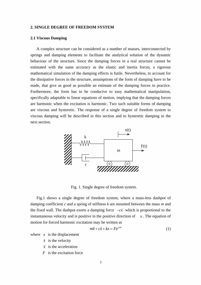
2. SINGLE DEGREE OF FREEDOM SYSTEM

2.1 Viscous Damping

A complex structure can be considered as a number of masses, interconnected by

springs and damping elements to facilitate the analytical solution of the dynamic

behaviour of the structure. Since the damping forces in a real structure cannot be

estimated with the same accuracy as the elastic and inertia forces, a rigorous

mathematical simulation of the damping effects is futile. Nevertheless, to account for

the dissipative forces in the structure, assumptions of the form of damping have to be

made, that give as good as possible an estimate of the damping forces in practice.

Furthermore, the form has to be conducive to easy mathematical manipulation,

specifically adaptable to linear equations of motion, implying that the damping forces

are harmonic when the excitation is harmonic. Two such suitable forms of damping

are viscous and hysteretic. The response of a single degree of freedom system to

viscous damping will be described in this section and to hysteretic damping in the

next section.

Fig. 1. Single degree of freedom system.

Fig.1 shows a single degree of freedom system, where a mass-less dashpot of

damping coefficient c and a spring of stiffness k are mounted between the mass m and

the fixed wall. The dashpot exerts a damping force cx which is proportional to the

instantaneous velocity and is positive in the positive direction of x . The equation of

motion for forced harmonic excitation may be written as

j tmx cx kx Fe (1)

where x is the displacement

x is the velocity

x is the acceleration

F is the excitation force

m

k

c

x(t)

F(t)

4

j is 1

and is the excitation frequency.

Dividing equation (1) by m one obtain

2 22 j t

n n n

Fx x x e

k

(2)

where n

k

m undamped natural frequency,

2 n c

c c

m c

dimensionless damping ratio,

cc is the critical damping.

Consider the solution of the form

j tx Xe

where X is the amplitude of the steady state vibration, it can be shown that

2

22 2

/ /

2 1 / 2 /

n

n n n n

F k F kX

j j

(3)

Thus

2

1

1 / 2 /

j tj t

n n

Fex Xe

kj

(4)

The displacement x is proportional to the applied force, the proportionality factor

being

2

1

1 / 2 /n n

Hj

(5)

which is known as the complex frequency response function (FRF). Equation (4)

illustrates that the displacement is a complex quantity with real and imaginary parts.

Thus

5

2

2 22 2 2 2

1 / 2 /

1 / 2 / 1 / 2 /

j tn n

n n n n

j Fex

k

(6)

This shows that the displacement has one real component

2

22 2

1 /Re

1 / 2 /

j tn

n n

Fex

k

(7)

which is in-phase with the applied force and another component

22 2

2 /Im

1 / 2 /

j t

n

n n

Fex

k

(8)

which has a phase lag of 90 behind the applied force.

The amplitude of the total displacement is given by

2 2

22 2

1Re Im

1 / 2 /

j t

n n

FeX X

k

(9)

The total displacement lags behind the force vector by an angle given by

1tan Im / Rex x, i.e.

1

2

2 /tan

1 /

n

n

(10)

The steady state solution of Eq.(2) can therefore also be written in the form

( )

22 2

1

1 / 2 /

j t

n n

Fex

k

(11)

where is given by Eq. (10).

The quantity in the square brackets of Eq. (11) is the absolute value of the

complex frequency response, H , and it is called the magnification factor, a

6

0

0.2

1

0.5

0.3

0.1

0

0.2

1 0.5 0.3

0.1

o180

o120

o150

o30

o60

o90

o0

dimensionless ratio between the amplitude of displacement X and the static

displacement F/k.

Fig. 2(a) Magnification factor H as a function of the dimensionless frequency

ratio / n for various damping ratio , and (b) phase lag of displacement behind

force as a function of .

(a)

(b)

7

Fig. 2(a) shows the absolute value of the complex frequency response function

H as a function of the dimensionless frequency ratio / n for various

damping ratio . It can be seen that increasing damping ratio tends to diminish

the amplitudes and to shift the peaks to the left of the vertical through / 1n . The

peaks occur at frequencies given by

21 2n (12)

where the peak value of H is given by

2

1

2 1H

(13)

For light damping ( < 5%) the curves are nearly symmetric about the vertical

through / 1n . The peak value of H occurs in the immediate vicinity of

/ 1n and is given by

1

2H Q

(14)

where Q is known as the quality factor.

Fig.2 (b) shows the phase angle against / n for various plotted from

Eq. (10). It should be noted that all curves pass through the point 90 ( / 2) ,

/ 1n ; i.e., no matter what the damping is, the phase angle between force and

displacement at the undamped natural frequency / n is 90 . Moreover, the phase

angle tends to zero for / 0n and to 180 for / n .

Consider the system with =10% for example, Fig.3.(a) defines the points 1P and

2P where the

8

d

nj

n

n

2 1 2 (15)n

2 1 12 (16)

n c

c

c Q

3dB

Peak

1P 2P

20

15

10

5

0

-5

-10

oX

k/F

(dB

)

0 0.2 0.4 0.6 0.8 1 1.41.2 1.81.6 2

/ n

Fig.3 (a) Magnification factor H as a function of the dimensionless frequency

ratio / n for 10% , and (b) complex s-plane of the poles.

amplitude of H reduces to / 2Q of its peak value are called the half power

points. If the ordinate is plotted on a logarithmic scale, 1P and 2P are points where

the amplitude of H reduces by 3 dB and are thus called the -3 dB points. The

difference in the frequencies of points 1P and 2P is called the 3 dB bandwidth of

the system, and for light damping it can be shown that

where is the 3 dB bandwidth

1 is the frequency at point 1P

2 is the frequency at point 2P

From Eqs. (14) and (15)

where is called the Loss Factor.

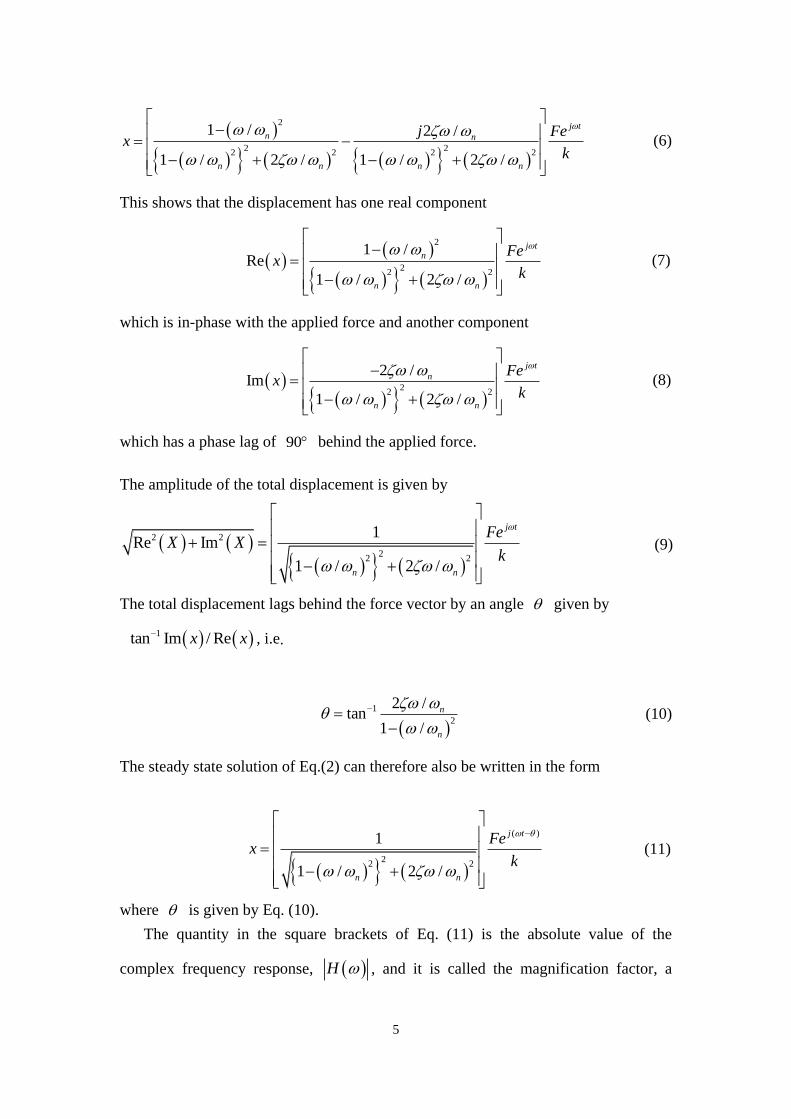
To examine the variation of the in-phase Re(x) and quadrature Im(x) components of

displacement, Eqs. (7) and (8) are plotted as a function of in Figs. 4(a) and 4(b)

respectively. The curves of the real component of displacement in Fig. 4(a) have a

(a) (b)

9

0.01

0.3

0.1

zero value at / 1n independent of damping ratio , and exhibits a peak and a

notch at frequencies

1

2

1 2

1 2

n

n

(17)

As the damping decreases, the peak and the notch increase in value and become

closer together. In the limit when 0 , the curve has an asymptote at / 1n .

The frequencies 1 and 2 are often used to determine the damping of the system

from the equation

2

2 1

2

2 1

/ 12

/ 1

(18)

The curves of the imaginary component of displacement have a notch in close

vicinity of / 1n and they are sharper than those of H in Fig. 2(a) for

corresponding values of .

(a)

10

0.01

0.3

0.1

Fig.4.(a) Real component of displacement as a function of the dimensionless

frequency ratio for various values of , and

(b) imaginary componen

t of displacement against for various values

of .

(b)

11

2.2 Hysteretic (structural) Damping

Another type of damping which permits setting up of linear damping equation,

and which may often give a closer approximation to the damping process in practice,

is the hysteretic damping, sometimes called structural damping. A large variety of

materials, when subjected to cyclic stress (for strains below the elastic limit), exhibit a

stress-strain relationship which is characterized by a hysteresis loop. The energy

dissipated per cycle due to internal friction in the material is proportional to the area

within the hysteresis loop, and hence the name hysteretic damping. It has been found

that the internal friction is independent of the rate of strain (independent of frequency)

and over a significant frequency range is proportional to the displacement. Thus the

damping force is proportional to the elastic force but, since energy is dissipated, it

must be in phase with the velocity (in quadrature with displacement).

Thus for simple harmonic motion the damping force is given by

x

j k x k

(19)

where is called the structural damping factor. The equation of motion for a single

degree of freedom system with structural damping can thus be written

j tk

mx x kx Fe

(20)

1 j tmx k j Fe (21)

where is called the complex stiffness.

The steady state solution of Eq. (21) is given by

2

1

1 /

j tj t

n

Fex Xe

kj

(22)

corresponding to Eq. (4) for viscous damping.

The real and the imaginary components of the displacement can be obtained:

2

2 22 22 2

1 /

1 / 1 /

j tn

n n

j Fex

k

(23)

12

1

0.2

0.5

0

Thus

2

22 2

1 /Re

1 /

j tn

n

Fex

k

(24)

and

22 2

Im

1 /

j t

n

Fex

k

(25)

The total displacement is given by

2

2 2

1

1 /

j t

n

Fex

k

(26)

which lags behind the force vector by an angle given by

1

2t a n

1 / n

(27)

(a)

13

1 0.2

0.5

0

o180

o120

o150

o30

o60

o90

o0

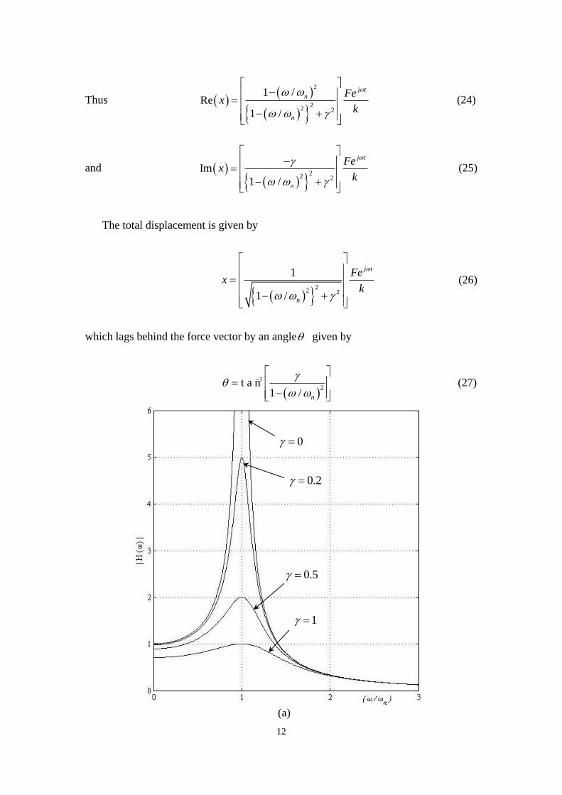
Fig.5 (a) Magnification factor as a function of / n for various values of the

structural damping factor , and (b) phase lag of displacement behind force as a

function of / n for various values of .

The term in the square brackets of expression (26) (magnification factor) and

are plotted against / n for various values of in Figs.5(a) and (b) respectively.

The curves of Figs.5(a) and (b) can be seen to be similar to those of Figs.2(a) and 2(b)

respectively for viscous damping; however, there are some minor differences. For

hysteretic damping it can be seen from Fig.5(a) that the maximum response occurs

exactly at / 1n independent of damping . At very low values of / n the

response for hysteretic damping depends on and the phase angle tends to 1tan whereas it is zero for viscous damping.

(b)

14

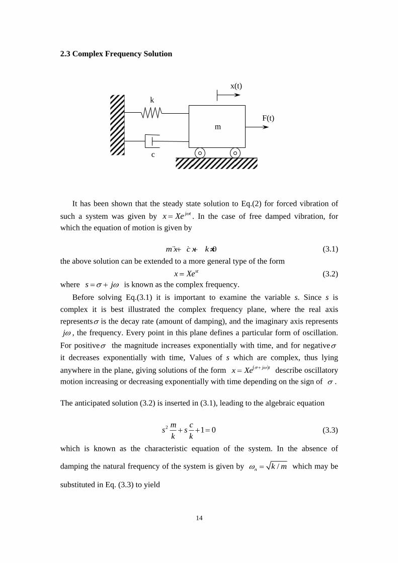
2.3 Complex Frequency Solution

It has been shown that the steady state solution to Eq.(2) for forced vibration of

such a system was given by j tx Xe . In the case of free damped vibration, for

which the equation of motion is given by

0m x c x k x (3.1)

the above solution can be extended to a more general type of the form

stx Xe (3.2)

where s j is known as the complex frequency.

Before solving Eq.(3.1) it is important to examine the variable s. Since s is

complex it is best illustrated the complex frequency plane, where the real axis

represents is the decay rate (amount of damping), and the imaginary axis represents

j , the frequency. Every point in this plane defines a particular form of oscillation.

For positive the magnitude increases exponentially with time, and for negative

it decreases exponentially with time, Values of s which are complex, thus lying

anywhere in the plane, giving solutions of the form j tx Xe

describe oscillatory

motion increasing or decreasing exponentially with time depending on the sign of .

The anticipated solution (3.2) is inserted in (3.1), leading to the algebraic equation

2 1 0m c

s sk k (3.3)

which is known as the characteristic equation of the system. In the absence of

damping the natural frequency of the system is given by /n k m which may be

substituted in Eq. (3.3) to yield

m

k

c

x(t)

F(t)

15

2

1 0n n

s c s

km

(3.4)

or

2

2 1 0n n

s s

(3.5)

where 1

2c

c c

c km is the damping ratio.

Since Eq. (3.5) is a quadratic, the two roots of the equation are given by

1 , 2 2 1n

s

(3.6)

and the values of s obtained, thus define two forms of oscillation in the complex plane.

Obviously the nature of the roots 1s and 2s depends on the value of .The effect

of the variation of on the roots can be illustrated in the complex plane (s-plane) in

the form of a diagram representing the locus of roots plotted as a function of the

parameter . From Eq. (3.6) it can be seen, that for 0 the roots are given by

1,2 ns j , which lie on the imaginary axis, corresponding to undamped oscillations

at the natural frequency of the system.

For 0 1 or 2c km which is known as the underdamped case, the roots are

given by

1 , 2 21n

sj

(3.7)

Thus 1s and 2s are always complex conjugate pairs, located symmetrically with

respect to the real axis. As the values of / ns are complex, the magnitude

2 21 1n

s

(3.8)

indicating that the locus of the roots is a circle of radius n , centered at the origin.

Furthermore, when the complex conjugate pairs of the roots are associated with each

other, they can be interpreted as a real oscillation, for example

16

2 cos

j t j t te e e t (3.9)

As approaches unity, 2c km the two roots approach the point n on the

real axis, which is known as the critically damped case.

For 1 or 2c km known as the overdamped case, the roots are given by

2

1,2 1n ns (3.10)

which lie on the negative real axis. As 1, 0s and 2s .

To obtain the time response of free vibration for given initial conditions, Eq.(3.6)

is substituted in Eq.(3.2) to give

1 2

1 2

s t s tx t X e X e (3.11)

For the overdamped case 1 , the solution is given by

2 21 1

1 2

n nt t

x t X e X e

i.e. 2 21 1

1 2

n nn

t tt

x t X e X e e

(3.12)

which describes aperiodic motion decaying exponentially with time. 1X and 2X

are determined from the initial displacement and velocity which in turn govern the

shape of the decaying curve.

For the critically damped case 1 , Eq. (3.5) has a double root 1 2 ns s

and the solution is given by

1 2nt

x t X tX e

(3.13)

The response again represents aperiodic motion decaying exponentially with time.

However, a critically damped system approaches the equilibrium position the fastest

for given initial conditions.

For the underdamped case 0 1 the solution is given by

2 21 1

1 2

n nn

j t j tt

x t X e X e e

17

i.e. 1 2d d nj t j t t

x t X e X e e

(3.14)

where 21d n is called the frequency of damped free vibration. Eq.(3.14)

represents exponentially decaying oscillatory motion with constant frequency d .

18

1F 2F

2x1x

1k2k 3k

1c 2c3c

3. MULTI–DEGREE OF FREEDOM SYSTEMS

3.1 FREE VIBRATION

The number of degrees of freedom chosen dictates the number of differential

equations necessary to characterize the system. As these equations are normally

coupled to each other, they must be decoupled before their solution is attempted. To

do this, the orthogonal properties of the Principal Modes are exploited, enabling the

original differential equations to be rewritten in terms of the principal coordinates.

However, in calculating the response under forced vibration, not only is it

necessary to make assumptions about the type of damping, but also the distribution of

damping--proportional or non-proportional. This is because the latter type of

distribution, generally encountered in complex structures, is considerably more

difficult to resolve mathematically, giving what is called complex modes, in contrast

to real modes obtained with proportional damping.

3.1.1 Natural Frequency and Vibration Mode

The equations of motion of the system shown in Fig.9 are

1 1 1 2 1 2 1 2 1 2 2 1

2 2 2 1 2 3 2 2 1 2 3 2 2

m x c c x cx k k x k x F

m x c x c c x k x k k x F

(3.1)

which can be written in matrix form as

1 2 2 1 2 21 1 1 1 1

2 2 3 2 2 32 2 2 2 2

0

0

c c c k k km x x x F

c c c k k km x x x F

(3.2)

To determine the natural frequencies and natural mode shapes of the system, the

undamped free vibration of the system is first considered. Thus the equations reduce

to

19

0m x k x (3.3)

where 1

2

0

0

mm

m

and 1 2 2

2 2 3

k k kk

k k k

Assuming harmonic motion { } { } j tx v e with 2 Eq. (3.3) becomes

0m x k x

or ( ) 0m k v (3.4)

Premultiplying Eq. (4.4) by 1

m

and rearranging we obtain

10m k I v

(3.5)

where 1

m k

is called a dynamic matrix and 1

m m I

is a unit matrix.

Eq. (3.5) is a set of simultaneous algebraic equations in v . From the theory of

equations it is known, that for a non-trivial solution {v} = 0, the determinant of the

coefficients of Eq. (3.5) must be zero. Thus

1

0m k I

(3.6)

which is known as the characteristic equation of the system. Eq. (3.6) when expanded

can be rewritten as

1 2

1 2 .......... 0n n n

na a a

(3.7)

which is a polynomial in for an n-degree-of-freedom system. The roots 1 of the

characteristic equation are called eigenvalues and the undamped natural frequencies

of the system are determined from the relationship

2

i i (3.8)

20

By substituting 1 into matrix equation (3.5) we obtain the corresponding natural (or

Principal) mode shape iv which is also called an eigenvector. The mode shape

represent a deformation pattern of the structure for the corresponding natural

frequency. As Eq. (3.5) are homogeneous, there is not a unique solution for the{ }v s.

Thus the natural mode shape is defined by the ratio of the amplitudes of motion at the

various points on the structure when excited at its natural frequency. The actual

amplitude on the other hand depends on the initial conditions and the position and

magnitude of the exciting forces.

Consider a numerical example for the system shown in Fig.9 where

1 2 1 2 35 ; 10 ; 2 / ; 4 /m kg m kg k k N m k N m

Substituting in Eq. (3.2) we get

1 1

2 2

5 0 4 2 0

0 10 2 6 0

x x

x x

(3.9)

Thus Eq. (3.5) becomes

1

1

2

5 0 4 2 1 0 0

0 10 2 6 0 1 0

v

v

1

2

4 / 5 2 / 5 0

1/ 5 3/ 5 0

v

v

(3.10)

For a non-trivial solution the determinant of the above equation must equal zero, thus

the characteristic equation

2 7 20

5 5

The roots of the above equation are

1,2 2 / 5 and 1

Thus 1 2 / 5 and 2 1 and the two natural frequencies are given by

21

1-

2

1

2For = rad/s the masses move in - phase

5

2For = 1 rad/s the masses move out -of - phase

1 1 2 22/ 5 and 1

Substitution of 1 and 2 in Eq. (3.10) will give the two natural mode shapes. Thus

the mode shape for the natural frequency 1 is 11

1

11

vv

v

where 11v is arbitrary.

Similarly the mode shape for the natural frequency 2 is 21

2

21 / 2

vv

v

For an arbitrary deflection of 11 21 1v v the two mode shapes would be

1

1

1v

for 1 2 / 5

and 2

1

1/ 2v

for 2 1

Fig. 10. Frequency and mode shapes for the two-degree-of-freedom system.

The system can thus vibrate freely with simple harmonic motion when started in the

correct way at one of two possible frequencies as shown in Fig.10. Note that the

masses move either in phase or 180 out of phase with each other. Since the masses

reach their maximum displacements simultaneously, the nodal points are clearly

defined.

1 1

1

1 1

1-

2

1

22

3.1.2 Orthogonal Properties of Eigenvectors

It was shown in the previous section that solution of Eq. (3.4) yields n eigenvalues

and n corresponding eigenvectors. Thus a particular elgenvalue i and the

eigenvector iv will satisfy Eq. (3.4); i.e,

i i ik v m v (3.11)

Premultiply Eq. (3.11) by the transpose of another mode shape jv , i.e.,

T T

j i i j iv k v v m v , where the superscript T denotes a transpose matrix.

We now write the equation for the thj mode and premultiply by the transpose of the

thi mode, i.e.,

T T

i j j i jv k v v m v (3.12)

As k and m are symmetric matrices

T T

j i i jv k v v k v

(3.13)

and T T

j i i jv m v v m v

(3.14)

Therefore subtracting Eq. (3.13) from Eq. (3.12) we obtain

0

T

i j i jv m v (3.15)

If i j (implying two different natural frequencies)

0

T

i jv m v

(3.16)

and from Eq. (3.13) it can be seen that

0

T

i jv k v

(3.17)

23

Equations (3.16) and (3.17) define the orthogonality properties of the mode shapes

with respect to the system mass and stiffness matrices respectively.

3.1.3 Generalized Mass and Generalized Stiffness

It can be seen that if i j in Eq. (3.15) then the two modes are not necessarily

orthogonal and Eq. (3.16) is equal to some scalar constant other than zero, e.g. im

1,2,3....

T

i i iv m v m i n (3.18)

and from Eq. (3.13) it follows that

2 1,2,3....

T

i i i i i i iv k v m m k i n (3.19)

im and ik are called the generalized mass and generalized stiffness respectively.

The numerical values of the mode shapes calculated above will be used to

determine the generalized mass and generalized stiffness. The mode shapes were

found to be

11

1v

for1 2 / 5 and 1

1

1/ 2v

for 2 1

Substituting 1v in Eq. (3.18) we obtain the generalized mass 1m for the first

mode: 1 15m .Similarly substituting 2v in Eq. (3.18) we obtain 2 15/ 2 .m

Thus the generalized masses 1m and 2m for the first and second modes are 15 and

15/2 respectively. The generalized stiffnesses 1k and 2k for the first and second

modes are 2

1 1 1 6k m and 2

2 2 2 2/15k m .

3.1.4 Normal Mode

If one of the elements of the eigenvector iv is assigned a certain value, the rest

of the 1n elements are also fixed because the ratio between any two elements is

constant. Thus the eigenvector becomes unique in an absolute sense. This process of

adjusting the elements of the natural modes to make their amplitude unique is called

normalization, and the resulting scaled natural modes are called orthonormal modes,

or normal modes. There are several ways to normalize the mode shapes, and the

24

common practice in engineering is that the mode shapes can be normalized such that

the generalized mass or modal mass im in Eq. (3.18) is set to unity. This method has

the advantage that Eq. (3.19) yields directly the eigenvalues i and thus the natural

frequencies.

The normalization will be illustrated by the numerical example of the system

shown in Fig.9. The mode shapes were shown to be

11

1

11

vv

v

for 1 2 / 5 and 21

2

21 / 2

vv

v

for 2 1

Therefore substitution of 1v in Eq. (3.18) yields

11 11

1

11 11

5 01

0 10

Tv v

mv v

And the normalized mode shape for 1 2 / 5 is

11

1

11

1/15

1/15

vv

v

(3.20)

Similarly for 2v we get 21 21

2

21 21

5 01

/ 2 / 20 10

Tv v

mv v

,and the

normalized mode shape for 2 1 is

21

2

21

2 /15

/ 2 2 / 5 / 2

vv

v

(3.21)

It can now be seen that these normalized mode shapes could also have been

obtained by dividing the natural modes by the square root of their respective

generalized masses calculated in the previous section, i.e., for normalization of the

first natural mode

25

1

1

1 1 1/151 1

1 115 1/15v

m

and for the second mode

2

2

1 1 2 /151 1

1/ 2 1/ 215/ 2 2 /15 / 2v

m

which are the same as calculated in Eq. (3.20) and (3.21) respectively.

3.2 Forced Vibration

The equations of motion of the two-degree-of-freedom system shown in Fig. 9

without damping can be written as

1 1

2 2

m x

m x

1 2 1

2 1

k k x

k x

2 2 1

2 3 2 2

k x F

k k x F

(3.22)

or in matrix form as

1 2 21 1 1 1

2 2 32 2 2 2

0

0

k k km x x F

k k km x x F

(3.23)

In solving the above equations for the response {x} for a particular set of exciting

forces, the major obstacle encountered is the coupling between the equations; i.e.,

both coordinates 1x and 2x occur in each of the Eq. (3.22). In Eq. (3.23) the

coupling is seen by the fact that while the stiffness matrix is symmetric, it is not

diagonal (i.e, the off-diagonal terms are non-zero). This type of coupling is called

elastic coupling or static coupling (non-diagonal stiffness matrix) and occurs for a

lumped mass system, if the coordinates chosen are at each mass point. If the equations

of motion had been written in terms of the extensions of each spring, the stiffness

matrix would have been diagonal but not the mass matrix. This kind of coupling is

termed inertial coupling or dynamic coupling (non-diagonal mass matrix). It is thus

seen that the way in which the equations are coupled depends on the choice of

coordinates. If the system of equations could be uncoupled, so that we obtained

diagonal mass and stiffness matrices, then each equation would be similar to that of a

single degree of freedom system, and could be solved independent of each other.

Indeed, the process of deriving the system response by transforming the equations of

motion into an independent set of equations is known as modal analysis.

26

Thus the coordinate transformation we are seeking, is one that decouples the

system inertially and elastically simultaneously, and therefore yields us diagonal mass

and stiffness matrices. It is here that the orthogonal properties of the mode shapes

discussed above come into use. It was shown by Eq. (3.18), that if the mass or the

stiffness matrix is post and pre-multiplied by a mode shape and its transpose

respectively, the result is some scalar constant. Thus with the use of a matrix v

whose columns are the mode shape vectors, we already have at our disposal the

necessary coordinate transformation. The x coordinates are transformed to by the

equation

x v p (3.24)

where

11 21 1

12 22 2

1 2

......

n

n

n n nn

v v v

v v vv

v v v

(3.25)

v is referred to as the modal matrix and p is called principal coordinates,

normal coordinates or modal coordinates. Eq. (3.23) can be written as

m x k x F (3.26)

and substituting Eq. (3.24) into (3.26) yields

m p k v p F

(3.27)

Pre-multiplying Eq. (3.26) by the transpose of the modal matrix, i.e, T

v , we obtain

T T Tv m v p v k v p v F

(3.28)

In Eq. (3.18) the mass matrix was post and pre-multiplied by one mode shape and

its transpose, giving a scalar quantity, while in Eq. (3.28) the mass matrix is post and

premultiplied by all the mode shapes and their transpose. Thus the product is a matrix

27

imi if

ik

M whose diagonal elements are some constants while all the off-diagonal terms

are zero, i.e.

Tv m v m

(3.29)

Similarly T

m k (3.30)

where m and k are diagonal matrices.

Hence Eq. (3.28) can be written as

Tm p k p v F (3.31)

Eq. (3.31) represents n-equations of the form

T

i i i i i im p k p v F f (3.32)

where iv is the thi column of the modal matrix, i.e., the

thi mode shape. im

and ik can be recognised as the thi modal mass (generalized mass) and

thi modal

stiffness (generalized stiffness) respectively. Eq. (3.32) is the equation of motion for

single degree of freedom systems shown in Fig.11.

Fig. 11. Single degree of freedom system defined by Eq. (3.32).

Since 2

i i ik m , Eq. (3.32) can be written as

28

2

T

iii i T

i i i

v Ffp p

m v m v (3.33)

Once the solution (time responses) of Eq. (3.31) for all ip is obtained, the

solution in terms of the original coordinates x can be obtained by transforming

back, i.e. substituting for i in Eq. (3.24) x v p . It should be noted that

when the modal matrix v of Eq. (3.25) is made up of columns of the normalized

mode shapes (such that 1im ). Eq. (3.33) would be simplified to

2 T

i i i i ip p f v F (3.34)

Thus the modal mass would be unity and the modal stiffness would be the square of

the natural frequency of the thi mode.

Let us consider our numerical example of the system of Fig.9 with forcing functions

1F and 2F . Thus Eq. (4.9) becomes

1 1 1

2 2 2

5 0 4 2

0 10 2 6

x x F

x x F

(3.35)

The natural frequencies and natural mode shapes were

1 1

2 2

12 / 5

1

11

1/ 2

v

v

Thus the modal matrix v using natural mode shapes

1 1

1 1/ 2v

The x coordinates are transformed by the equation

29

x v p (3.36)

i.e. 1 1

2 2

1 1

1 1/ 2

x p

x p

(3.37)

Substituting Eq. (4.41) into Eq. (4.40) and pre-multiplying by T

v gives

1 1 1

2 2 2

5 0 4 2

0 10 2 6

T T Tp p Fv v v v v

p p F

The products T

v m v and T

v k v are calculated to be

1 1 5 0 1 1 15 0

1 1/ 2 0 10 1 1/ 2 0 15 / 2

1 1 4 2 1 1 6 0

1 1/ 2 2 6 1 1/ 2 0 15 / 2

T

T

v m v

v k v

Substituting these products into the equation above we obtain

1 1 1

2 2 2

15 0 6 0 1 1

0 15/ 2 0 15/ 2 1 1/ 2

p p F

p p F

Thus the equations of motion in are

1 1 1 2

2 2 1 2

15 6

15/ 2 15/ 2 / 2

p p F F

p p F F

(3.38)

The original set of equations (3.38) are shown to be uncoupled; in other words the two

degree of freedom system is broken down to two single degree of freedom systems

shown in Fig.12.

30

1 1 2F F 15/22 1 2 / 2F F

15/2

422

10

6

5

15

1F 2F

2x1x

5

Fig. 12. The undamped two-degree-of-freedom system shown in Fig. 9, is

transformed into two single degree of freedom systems.

As mentioned above, the modal matrix can also be made up of columns of the

normalized mode shapes (such that 1im ). Using the normalized mode shapes from

Eqs. (3.20) and (3.21), the normalized modal matrix v is given by

1/15 2 /15

1/15 2 /15 / 2v

Thus the products T

v m v and T

v k v are given by

1 / 1 5 1 / 1 5 5 0 1 / 1 5 2 / 1 5 1 0

0 1 0 0 12 / 1 5 2 / 1 5 / 2 1 / 1 5 2 / 1 5 / 2

Tv m v

1 / 1 5 1 / 1 5 4 2 1 / 1 5 2 / 1 5 2 / 5 0

2 6 0 12 / 1 5 2 / 1 5 / 2 1 / 1 5 2 / 1 5 / 2

Tv k v

It can thus be seen that, by using the normalized modal matrix for coordinate

transformation, the mass matrix becomes a unit matrix and the stiffness matrix is

diagonalized with the diagonal terms equal to the eigenvalues (the square of the

natural frequencies).

31

In general 1T

v m v

and T

v k v

where

1

2

00 0...

00 0...

0 0 ... n

Once the time responses for 1p and 2p have been determined from Eq. (3.38),

they can be substituted in Eq. (3.37) to give the time response in terms of the original

coordinates x, thus

1 1 2

2 1 2

1

2

x t p t p t

x t p t p t

(3.39)

Eq. (3.39) in fact illustrates a very important principle in vibration, namely that any

possible free motion can be written as the sum of the motion in each principal mode

in some proportion and relative phase. In general for an n-degree-of-freedom system

1 11 21 1

2 12 22 2

1 1 1 2 2 2

1 2

cos cos ... cos

n

n

n n n

n n n nn

x v v v

x v v vp t p t p t

x v v v

(3.40)

If the two-degree-of-freedom system discussed above is given arbitrary starting

conditions, the resulting motion would be the sum of the two principal modes in some

proportion and would look as shown in Fig.13.

32

Fig. 13. Response of the two-degree-of-freedom system when given arbitrary starting

conditions.

3.3 Proportional Damping

The assumption that systems have no damping is only hypothetical, since all

structures have internal damping. As there are several types of damping, viscous,

hysteretic, coulomb, aerodynamic etc., it is generally difficult to ascertain which type

of damping is represented in a particular structure. In fact a structure may have

damping characteristics resulting from a combination of all the types. In many cases,

however, the damping is small and certain simplifying assumptions can be made.

3.3.1 Viscous Damping

The equations of motion of the two degree of freedom system with damping, shown

in Fig. 9, are given by Eq. (3.2)

1 2 2 1 2 21 1 1 1 1

2 2 3 2 2 32 2 2 2 2

0

0

c c c k k km x x x F

c c c k k km x x x F

(3.41)

In short form they can be written as

33

m x c x k x F (3.42)

Two assumptions are taken for granted before attempting solution of these equations.

Firstly, that the type of damping is viscous, and secondly that the distribution of

damping is proportional. By proportional damping it is implied that the damping

matrix [c] is proportional to the stiffness matrix or the mass matrix, or to some linear

combination of these two matrices. Mathematically it means that either

or orc m c k c m k

(3.43)

where and are constants.

Because of the assumption of proportional damping, the coordinate transformation

using the modal matrix for the free undamped case which diagonalizes the mass and

stiffness matrices, will also diagonalize the damping matrix. Thus the coupled

equations of motion for a proportionally damped system can also be uncoupled to

single degree of freedom systems as shown in the following.

Substituting the coordinate transformation of Eq. (3.24) into Eq. (3.42) we obtain

m v p c v p k v p F (3.44)

Pre-multiplying Eq. (3.44) by the transpose of the modal matrix, i.e, T

v we obtain

T T T T

v m v p v c v p v k v p v F (3.45)

It was shown before in Eq. (3.29) and (3.30) that because of the orthogonal properties

of the mode shapes the mass and stiffness matrices are diagonalized, i.e.

Tv m v m

and T

v k v k

Because of proportional damping i.e.

c m k

we have T T

v c v v m k v

34

imi if

ik ic

T T

v m v v k v

i.e. T

v c v m m c where c is a diagonal matrix.

Thus substitution into Eq. (3.45) gives

Tm p c p k p v F (3.46)

Eq. (3.46) represents an uncoupled set of equations for damped single degree of

freedom systems. The thi equation is

T

i i i i i i i im p c p k p v F f (3.47)

which represents the equation of motion of a single degree of freedom system.

Fig. 14. Single degree of freedom system defined by Eq. (3.47)

Since 2

i i ik m , from Eq. (3.19), Eq. (3.47) can be written as

22

T

i ii i i i i i

i i

v F fp p p

m m

(3.48)

Where 2

ii

i i

c

k m

(3.49)

The solution of a damped single degree of freedom system, as described by Eq. (3.48)

has been discussed previously. Once the solution of Eq. (3.48) is obtained for all ip ,

35

the solution in terms of the original coordinates x can be deduced by transforming

back, i.e. substituting for ip . in Eq. (3.24).

It should be noted that if the damping matrix is proportional to the stiffness matrix, i.e,

c k then from Eq. (3.48) we see that

ii i

i i

k

k m

which means that the higher frequency modes will have higher damping ratios.

3.3.2 Hysteretic Damping

Hysteretic or structural damping was discussed under single degree of freedom

systems. It was shown, that in this case the damping force is proportional to the elastic

force, but as energy is dissipated, the force is in phase with the velocity. Thus for

simple harmonic motion the damping force is given by j kx . For a multi-degree of

freedom system, the equations of motion with hysteretic damping can be written as

m x j k x k x F (3.50)

Changing to Principal Coordinates as shown in the section above leads to

1

Tm p j k p v F (3.51)

Thus each equation is of the form

1

T

i i i i im p j k p v F

i.e. 21

T

i

i i i

i

v Fp j p

m (3.52)

If j tF F e

then j tp p e

Substituting in Eq. (3.52) we obtain

2 21

T

i ii i i i

i i

v F Fp j p

m m (3.53)

36

the solution of which has been discussed previously.

3.4 Non-proportional Damping

3.4.1 State-Space Method

When the damping matrix is not proportional to the mass or the stiffness matrix,

neither the modal matrix nor the weighted modal matrix will diagonalize the damping

matrix. In this general case of damping, the coupled equations of motion have to be

solved simultaneously, or they need to be uncoupled using the state-space method. By

this method the set of n second order differential equations are converted to an

equivalent set of 2n first order differential equations, by assigning new variables

(referred to as state variables) to each of the original variables and their derivatives.

To illustrate the procedure, the equations of motion for the two degree of freedom

system shown in Fig.9 are written as

1 1

2 2

0

0

m x

m x

1 1

2 2

0

0

m x

m x

0

0

1 1 1 2 2 1 1 2 2 1 1

2 2 2 1 2 2 2 1 2 2 2

0

0

m x c c c x k k k x F

m x c c c x k k k x F

(3.54)

or in partitioned matrix form as

1 1 1 1

2 2 2 2

1 1 2 2 1 1 2 2 1

2 2 1 2 2 2 1 2 2

0 00 0 0 0

0 00 0 0 0

0 0 0

0 0 0

m x m x

m x m x

m c c c x k k k x

m c c c x k k k x

1

2

0

0

F

F

Substituting

1 1

2 2

x z

x z

1 1 3

2 2 4

x z z

x z z

1 3

2 4

x z

x z

we get

37

1 1 2 2 1 1 2 2 1

2 2 1 2 2 2 1 2 2

1 3 1 3

2 4 2 4

0 0 0

0 0 0

0 00 0 0 0

0 00 0 0 0

m c c c z k k k z

m c c c z k k k z

m z m z

m z m z

1

2

0

0

F

F

(3.55)

which can be abbreviated to

A z B z Q (3.56)

It can be seen that while the second order equations have been reduced to first order

equations, the number of equations have been doubled.

The solution of above equations for free vibration reveals that damped natural

modes do exist, however, they are not identical to the undamped natural modes. For

the undamped modes, various parts of the structure move either in phase or 180

out-of-phase with each other. For the non-proportionally damped structures, there are

phase differences between the various parts of the structure, which result in complex

mode shapes. This difference is manifested by the fact that for undamped natural

modes all points on the structure pass through their equilibrium positions

simultaneously, which is not the case for the complex modes. Thus the undamped

natural modes have well-defined nodal points or lines and appear as a standing wave,

while for complex modes the nodal lines are not stationary.

3.4.2 Forced Normal Modes of Damped Systems

For an n-degree-of-freedom system with viscous damping, the equations of

motion for steady state sinusoidal excitation can be written in its general form as

sinm x c x k x F t (3.57)

where the system inertia, damping and stiffness matrices [m], [c] and [k] respectively,

and they are assumed to be real symmetric and positive definite. If the damping is

hysteretic, the second term would be given by 1/ d x , where [d] is the hysteretic

damping matrix. In the general case damping would be non-proportional and thus the

damping matrix cannot be diagonalized using the normal mode transformation. For an

38

arbitrary set of forces F and excitation frequency the solution of Eq. (3.57) is

rather complicated.

Although the responses at each coordinate x are harmonic with the excitation

frequency, they are not all in phase with each other or with the excitation force. If,

however, a system with n-degree-of-freedom is excited by n number of forces which

are either 0 or 180 out-of-phase (often called monophase or coherently phased

forces), then for a particular ratio of forces, the response at each of the coordinates

will be in phase with each other and lag behind the force by a common angle

(called the characteristic phase lag). Thus we have to determine the conditions which

will produce a solution of the form

1 1

2 2

3 3 sin sin

n n

x X

x X

x X t v t

x X

(3.58)

For any given excitation frequency , there exist n solutions of the type given by Eq.

(3.58), where each of the modes v is associated with a definite phase i and a

corresponding distribution of forces i

which is required for its excitation. The

response under these conditions is called the “forced normal modes” of the damped

system, since every point of the system moves in phase and passes through its

equilibrium position simultaneously with respect to the other points.

Substituting Eq. (3.58) in Eq. (3.57) gives

2sin cos sint k m v t c v F t

(3.59)

Expanding the sin t and the cos t terms and separating the sin t

and cos t terms we obtain

2cos sink m v c v F

(3.60)

39

2sin cos 0k m v c v

(3.61)

These equations contain three unknowns F , v and since is given. If

cos 0 , Eq. (3.61) may be divided by cos to give

2tan 0k m c v

(3.62)

Eq. (3.62) has a non-trivial solution if the determinant

2tan 0k m c (3.63)

It is evident that for a given there are n values of tan 1,2,i i n corresponding

to the n eigenvalues and for each tan i there is a corresponding eigenvector i

v

satisfying the equation

2tan 0i ik m c v

(3.64)

If Eq. (3.64) is premultiplied by the transpose T

iv and rearranged, we obtain

2tan

T

i ii T

i i

v c v

v k m v

(3.65)

From Eq. (3.65) it can be seen that each of the roots tan i is a continuous

function of . For low values of , tan i is small, i.e, i is a small angle. As

increases and approaches 1 the undamped natural frequency, one of the roots

i (which can be named i ) approaches the value / 2 . As is increased above

1 the denominator of Eq. (3.65) gets negative and 1 gets larger than / 2 .

When tends to , 1 tends to . In a similar manner the remaining roots

i 2 , 3 ,i n can be plotted as a function of frequency , where

2,3,i i n is equal to / 2 at the ith undamped natural frequency i . Thus

40

k is that root which has the value / 2 at the undamped natural frequency

k .

Having examined the variation of eigenvalues tan i as a function of

frequency, the mode shapes can now be investigated. It can be seen from Eqs. (3.63)

and (3.64) that at any one frequency the mode shapes depend only on the shape of the

damping matrix and not on its intensity. If every element in the matrix [c] is

multiplied by a constant factor, then Eq. (3.63) shows that the roots tan i will all be

increased by the same ratio. Thus Eq. (3.64), which determines the mode shapes, will

be multiplied throughout by the same factor and the mode shape i

v will be

unchanged. Eq. (3.64) can be re-written as

2 0t a n i

i

ck m v

(3.66)

When is equal to one of the undamped natural frequencies, say 1 , then one

of the roots is 90 as shown above. Thus Eq. (3.66) which determines the mode

shape for this root becomes

2

1 10k m v (3.67)

It can thus be seen, that when the frequency is equal to one of the undamped natural

frequencies, the mode shape for one of the roots (which is equal to / 2 ) is identical

to the Principal or Normal mode shape.

Attention can now be paid to the force ratio that is required to excite any one

mode i

v for the corresponding root tan i at any one frequency. The force ratio

required can be calculated from Eq. (3.60) namely

2cos sini ii i ik m v c v (3.68)

In the special case when 1 one of the undamped natural frequencies, one of the

roots 1 90i and Eq. (3.68) reduces to

1 1 1c v (3.69)

41

4N/m2N/m2N/m

1 sinF t 2 sinF t

2x1x

7c Ns/m1c Ns/m4c Ns/m

To illustrate the concepts discussed above consider the same numerical example of

the two degree of freedom system of Fig. 9, but with the values of damping added as

shown in Fig. 16.

Fig. 16. Two degree of freedom system with non-proportional damping.

Thus the equations of motion according to Eq. (3.1) become

1 1 1 1

2 2 2 2

5 0 5 1 4 2sin

0 10 1 8 2 6

x x x Fc ct

x x x Fc c

For a non-trivial solution the determinant of Eq. (3.63) must be equal to zero, i.e.

24 2 5 0 5 1

tan 02 6 0 10 1 8

c

i.e,

2

2

tan 4 5 5 tan 20

tan 2 tan 6 10 8

c c

c c

i.e, 22 2tan 4 5 5 tan 6 10 8 tan 2 0c c c

which reduces to

2 4 2 2 2 220 70 50 tan 2 29 45 tan 39 0c c

(3.70)

The undamped natural frequencies of the system are given by letting c = 0, i.e., by the

equation

2 420 70 50 0

42

They are found to be 1 2 / 5 0.63 rad/s and

2 1 rad/s, which obviously

should be the same as those calculated under section 3.1.

Dividing Eq. (3.70) by 2tan and substituting

tan

c

we get

2 2 2 439 2 29 45 20 70 50 0

The roots of this equation are given by

2

2 2 2 429 45 29 45 39 20 70 50

tan 39

c

(3.71)

When is equal to one of the undamped natural frequencies 1 or 2 the

equation reduces to

2 229 45 29 45

tan 39

c

Thus when 1 we get

2 2

129 45 29 45

tan 39

c

so that 1 90 for the negative sign and

1 12 2

1

39tan

2 29 45

c

for the positive sign.

Similarly when 2 we get

2 2

2 2229 45 29 45

tan 39

c

so that 2 90 for the negative sign and

43

1 21 2

2

39tan

2 29 45

c

for the positive sign.

The variation of 1 and 2 can be plotted as a function of frequency using Eq.

(3.71). The curves are shown in Fig.17 for three values of damping c, corresponding

roughly to light, medium and heavy damping. The shape of the curves are seen to be

similar to those of Fig.2(b).

Fig. 17. Variation of the roots 1 and 2 as a function of frequency for three values

of damping.

The mode shapes are obtained by substituting numerical values for the matrices

[m], [c] and [k] in Eq. (3.64), i.e,

12

2

4 2 5 0 5 1 0tan

2 6 0 10 1 8 0i

i

vc

v

i.e.

2

1

22

tan 4 5 5 tan 2 0

0tan 2 tan 6 10 8

i i

ii i

c c v

vc c

(i= 1, 2)

Expanding the first equation we get

2

1 2tan 4 5 5 tan 2 0i ic v c v

44

1

2 1

v

v

1

2 2

v

v

11

2

1v

v

12

2

2v

v

Thus

1

2 22

2 tan 2 / tan

tan 4 5 5 4 5 5 / tan

i i

i ii

c cv

v c c

Substituting for / tanc from Eq. (3.71) we obtain

2 2 4

1

2 2 42

49 45 61 120 75

11 30 5 61 120 75i

v

v

(3.72)

Fig.18. The characteristic phase lag modes as a function of frequency

The characteristic phase lag modes are plotted as a function of frequency using Eq.

(3.72) in Fig.18. The positive sign now corresponds to i = 1 for the first mode and the

negative sign corresponds to i = 2 for the second mode. Note, in the special case when

is equal to the first undamped natural frequency 1 2 / 5 for i = 1 we obtain

1

11

12

1v

vv

which is the same as the first principal mode shape 1

v .

45

At 1 2 / 5 for i = 2 we obtain

1

56

32v

Similarly, when is equal to the second undamped natural frequency 2 1 for i

= 1 we obtain

2

110

121v

At 2 1 for i = 2 we obtain

2

2

1v

which is the same as the second principal mode shape 2

v .

The force ratio required to excite any one mode i

v for the corresponding root

tan i at any one frequency can be calculated from Eq. (3.68), i.e.,

1 1 12

2 2 2

4 2 5 0 5 1cos sin

2 6 0 20 1 8i i

i i

v v Fc

v v F

(3.73)

The force ratio for each root can be plotted as a function of frequency by substituting

the value of for each and the corresponding mode shape. Fig.19 shows the

force ratios required as a function of frequency for the two s .

46

Fig. 19. Force ratios required to excite the two modes as a function of frequency.

It is, however, interesting to calculate the force ratios at the undamped natural

frequencies. As shown previously, at any one undamped natural frequency, one of the

roots tan i , i.e, one of the 90i , and for that root the mode shape obtained is

the Principal Mode Shape. Thus Eq.(3.73) reduces to

1 1

2 2

5 1

1 8

v Fc

v F

which gives the force ratio required to excite the principal mode shape at the

corresponding undamped natural frequency.

Substituting the first undamped natural frequency 1 2 / 5 and 1 2/ 1v v we

obtain

1

2

5 1 12 / 5

1 8 1

Fc

F

i.e,

1 2 1/ 4 / 7F F

47

Substituting the second undamped natural frequency 2 1 and 1 2/ 2 /1v v

we obtain

1

2

5 1 21

1 8 1

Fc

F

i.e,

1 2 2/ 11/10F F

Before concluding this section it is important to recapitulate the following points:

(1) For each frequency of excitation there are as many characteristic phase angles as

there are number of degrees of freedom, corresponding to certain sets of forces.

(2) For each characteristic phase lag there is a corresponding mode shape which

varies with frequency. At the undamped natural frequencies one of the mode shapes

is identical to the corresponding undamped Principal mode.

(3) The mode shapes depend on the shape of the damping matrix and not on the

intensity of damping.

(4) In each mode the responses at the coordinates are all in phase, but lag behind the

excitation force by an angle . At the undamped natural frequency, 0 90 for

one of the modes which is the principal mode.

(5) Orthogonal properties of phase lag modes also exist.

The orthogonal properties of the principal modes of vibration were demonstrated

previously in section 3.1.3. To derive analogous properties of forced modes. Eq.(3.62)

can be written for the ith eigenvalue and eigenvector and premultiplied by the

transpose of the j th eigenvector. The procedure is repeated with i and interchanged

giving the following two equations,

2tan 0

T T

i j i j iv k m v v c v

(3.74)

2tan 0

T T

j i j i jv k m v v c v

(3.75)

Since [m], [c] and [k] are symmetric matrices Eq.(3.75) can be transposed to obtain

48

2tan 0

T T

j j i j iv k m v v c v

(3.76)

Subtracting Eq.(3.76) from Eq.(3.74) we obtain the orthogonal properties as

2 0

T

j iv k m v (3.77)

And 0T

j iv c v

(3.78)

provided tan tani j .

Combining Eqs.(3.77) and (3.78) with Eq.(3.60) we obtain the third relation

0

T T

i jj iv F v F

(3.79)