Unit II Quiz Question Sampler 2.086/2.090 Fall 2012

You may refer to the text and other class materials as well as your own notes and scripts.

For Quiz 2 (on Unit II) you will need a calculator (for arithmetic operations and standard func­tions); note, however, that laptops, tablets, and smartphones are not permitted.

To simulate real quiz conditions you should complete all the questions in this sampler in 90 minutes.

NAME

There are a total of 100 points: five questions, each worth 20 points.

All questions are multiple choice; in all cases circle one and only one answer.

We include a blank page at the end which you may use for any derivations, but note that we do not refer to your work and in any event your grade is determined solely by your multiple choice selections.

You may assume throughout this quiz that all arithmetic operations are performed exactly (with no floating point truncation or round-off errors). We may display the numbers in the multiple-choice options to just a few digits, however you should always be able to clearly discriminate the correct answer from the incorrect answers.

1

Question 1 (20 points). In this question we consider a discrete random variable X which can take on three values, −1 or 0 or 1, according to the probability mass function fX (x) given by ⎧ ⎨ 1/3 x = −1

fX (x) = 1/3 x = 0 . (1)⎩ 1/3 x = 1

We recall that fX (x) is the probability that the random variable X takes on the value x. We also consider a second random variable Y which is a function of X: Y = X2, or equivalently

0 if X = 0 Y = . (2)

1 if X = −1 or X = 1

Note that Y can take on only two values, either 0 or 1.

(i) (6 points) The mean of X is

(a) -1/6

(b) 0

(c) 1/2

(d) 2/3

(e) 1

(ii) (6 points) The standard deviation of X is

(a) 1

(b) 0.4714

(c) 0

(d) 0.8165

(e) 0.5000

Note we are asking for the standard deviation, not the variance.

2

(iii) (4 points) The mean of Y is

(a) -1/6

(b) 0

(c) 1/2

(d) 2/3

(e) 1

(iv) (4 points) The standard deviation of Y is

(a) 1

(b) 0.4714

(c) 0

(d) 0.8165

(e) 0.5000

Note we are asking for the standard deviation, not the variance.

3

Question 2 (20 points). Victory in a football game can be affected by which team wins the coin flip (also known as the coin toss). We consider the case of a particular team, say the New England Patriots. We denote by COIN a random “variable” which represents the result of the coin flip. The random variable COIN can take on two “values” (or outcomes): COIN = WIN FLIP — the Patriots win the coin flip; COIN = LOSE FLIP — the Patriots lose the coin flip. We denote by FINAL a random “variable” which represents the result of the game. The random variable FINAL can take on two “values” (or outcomes): FINAL = WIN GAME — the Patriots win the game; FINAL = LOSE GAME — the Patriots lose the game.

You are given the following conditional probabilities: P(FINAL = WIN GAME | COIN = WIN FLIP) = 0.92; P(FINAL = WIN GAME | COIN = LOSE FLIP) = 0.82. We shall further assume that the coin is “fair”: we are given the marginal probability P(COIN = WIN FLIP) = 0.50. (Note that the data for this problem is entirely fictitious, and of course our model is very simplistic.)

(i) (8 points) The marginal probability P(FINAL = WIN GAME) is

(a) 0.50

(b) 0.92

(c) 0.87

(d) 0.82

(ii) (6 points) The conditional probability P(COIN = LOSE FLIP | FINAL = WIN GAME) is

(a) 0.080

(b) 0.820

(c) 0.471

(d) 0.446

4

(iii) (6 points) Over the course of many seasons and hence may games in what fraction (expressed as a percentage) of the total games played do the Patriots lose the coin flip and win the game (i.e., both events occur)? (For example, if the Patriots play 100 games, and in 20 of these games the Patriots lose the coin flip and win the game, then the fraction is 20%.)

(a) 87%

(b) 47%

(c) 41%

(d) 50%

You should choose the answer which is most likely (in the limit of many games). Hint: Consider the appropriate joint probability and then apply the frequentist interpretation of probabilities.

5

Question 3 (20 points) A company manufactures a widget which contains a hole for a wire bundle. The customer will accept the widgets only if at least 98% of the (many) widgets delivered have a hole radius r greater than 0.1 cm. The widget company decides to a perform a test prior to shipment to the customer.

A quality control engineer at the widget company draws a random sample of n = 2000 (independent) widgets and proceeds to measure the hole radius of each widget. It is found that, of these 2000 randomly chosen widgets, 1990 of the widgets do indeed have a hole radius greater than 0.1 cm; the remaining 10 widgets have a hole radius less than (or equal to) 0.1 cm.

To model this situation we introduce a Bernoulli random variable B: a hole radius R less than or equal to 0.1 cm is encoded as a 0 and occurs with probability 1 − θ; a hole radius R greater than 0.1 cm is encoded as a 1 and occurs with probability θ. Here R is the random variable which represents the hole radius which in turn determines the Bernoulli random variable.

(i) (8 points) Based on the experimental data from the sample of n = 2000 widgets, the sample mean estimate for θ is

(a) 0.950

(b) 0.995

(c) 0.980

(d) 0.005

(ii) (8 points) Based on the experimental data from the sample of n = 2000 widgets, the (two– sided) normal–approximation confidence interval for θ at confidence level γ = 0.95 is given by

(a) [0.8568, 1.1332]

(b) [0.9934 ,0.9966]

(c) [0.9919, 0.9981]

(d) can not be evaluated as the normal-approximation criteria are not satisfied

(iii) (4 points) From your result of part (ii) can you conclude with confidence level 0.95 that 98% of the (very many) widgets delivered to the customer will have hole radius greater than 0.1 cm?

(a) Yes

(b) No

Note you may assume here that our random model for the widget hole radius R and hence Bernoulli variable B is valid (as only in this case can you make rigorous statistical inferences).

6

Question 4 (20 points). Consider the following Matlab script

% begin script

clear % note we "clear" the workspace, % and hence no variables are shared between the different scripts in this quiz

n = 10000; % number of random darts

u1 = rand(1,n); u2 = rand(1,n);

x1 = 1 + u1; x2 = 3*u2;

multfac = 2.0;

numinside = sum( x2 <= f_of_x(x1,multfac) );

area_estimate = (numinside/n)*3.0;

% end script

and function f_of_x

function [value] = f_of_x(x,const)

value = zeros(1,length(x)); for i = 1:length(x)

value(i) = const/x(i); end

return end

for approximating an area AD of a domain D by the Monte Carlo method. In the limit that n tends to infinity, area_estimate will approach AD.

7

(i) (10 points) Each of the bivariate uniform random variates (realizations of random variables from the bivariate uniform density) (x1(i),x2(i)), i = 1, . . . , n, resides in the rectangle

(a) 0 ≤ x1(i) ≤ 1, 0 ≤ x2(i) ≤ 3

(b) 0 ≤ x1(i) ≤ 1, 0 ≤ x2(i) ≤ 2

(c) 1 ≤ x1(i) ≤ 2, 0 ≤ x2(i) ≤ 3

(d) 1 ≤ x1(i) ≤ 2, 0 ≤ x2(i) ≤ 2

(ii) (10 points) The area AD is given by

(a) 2.000

(b) 0.693

(c) 1.387

(d) 3.000

Hint : draw a sketch in which you indicate the rectangle over which x1,x2 is defined (i.e., at which you throw your darts); then include in your sketch the domain D defined by the conditional x2 <= f_of_x(x1,multfac); finally, recall the area interpretation of the definite integral (and perform the integral) to determine AD.

8

Question 5 (20 points). Consider the following Matlab script

% begin script

clear % note we "clear" the workspace, % and hence no variables are shared between the different scripts in this quiz

n = 100000; % number of random darts

u1 = rand(1,n); u2 = rand(1,n);

x = 10*u1; y = u2; x_exp = [];

for i = 1:n if( y(i) <= EXPR1 ) % EXPR1 to be chosen below

x_exp = EXPR2; % EXPR2 to be chosen below end

end

% end script

which is intended to provide random variates from the exponential density function, fX (x) = e−x , 0 ≤ x ≤ 10, based on the acceptance-rejection method. (The “true” exponential density can actually take on any value x over 0 ≤ x ≤ ∞. However, e−10 is extremely small, so we can just consider a truncated interval 0 ≤ x ≤ 10.)

(i) (5 points) The expression EXPR1 should be

(a) n

(b) exp(-x(i))

(c) exp(-y(i))

(d) x(i)

9

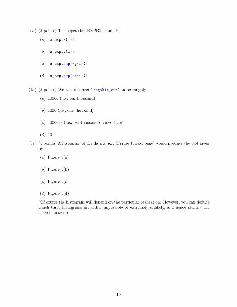
(ii) (5 points) The expression EXPR2 should be

(a) [x_exp,x(i)]

(b) [x_exp,y(i)]

(c) [x_exp,exp(-y(i))]

(d) [x_exp,exp(-x(i))]

(iii) (5 points) We would expect length(x_exp) to be roughly

(a) 10000 (i.e., ten thousand)

(b) 1000 (i.e., one thousand)

(c) 10000/e (i.e., ten thousand divided by e)

(d) 10

(iv) (5 points) A histogram of the data x_exp (Figure 1, next page) would produce the plot given by

(a) Figure 1(a)

(b) Figure 1(b)

(c) Figure 1(c)

(d) Figure 1(d)

(Of course the histogram will depend on the particular realization. However, you can deduce which three histograms are either impossible or extremely unlikely, and hence identify the correct answer.)

10

0 1 2 3 4 5 6 7 8 9 100

500

1000

1500

2000

2500

3000

3500

4000

4500

5000

frequency

0 1 2 3 4 5 6 7 8 9 100

500

1000

1500

2000

2500

frequency

(a) (b)

−30 −20 −10 0 10 20 300

1000

2000

3000

4000

5000

6000

7000

8000

frequency

0 1 2 3 4 5 6 7 8 9 100

200

400

600

800

1000

1200

1400

1600

1800

frequency

(c) (d)

Figure 1: Candidate histograms. Note “frequency” here refers to the number of variates that take on a value in a given bin (there are 50 bins, and hence for example in Figure 1(b) the first bin is defined as 0 ≤ x < 10/50(= .2)).

11

Answer Key

Q1 (i) (b) 0 (ii) (d) 0.8165 (iii) (d) 2/3 (iv) (b) 0.4714

Q2 (i) (c) 0.87 (ii) (c) 0.471 (iii) (c) 41%

Q3 (i) (b) 0.995 (ii) (c) [0.9919, 0.9981] (iii) (a) Yes

Q4 (i) (c) 1 ≤ x1(i) ≤ 2, 0 ≤ x2(i) ≤ 3 (ii) (c) 1.387

Q5 (i) (b) exp(-x(i)) (ii) (a) [x_exp,x(i)] (iii) (a) 10000 (iv) (d) Figure 1(d)

12

MIT OpenCourseWarehttp://ocw.mit.edu

2.086 Numerical Computation for Mechanical EngineersFall 2012

For information about citing these materials or our Terms of Use, visit: http://ocw.mit.edu/terms.