II Neutral Atomic Hydrogen (HI) Regions

II-1

II Neutral Atomic Hydrogen (HI) Regions

This chapter discusses the physics of regions dominated by neutral (or only weakly ionized) atomic species. Since neutral atomic hydrogen is the dominant species, we generically refer to such gas as “Neutral Hydrogen” or “HI” Regions, but bear in mind that the gas also contains metals in neutral and weakly ionized forms that play an important role.

II-1 Interstellar UV & Visible Absorption Lines The first observational evidence for an all-pervasive ISM came from observations of visible-wavelength absorption lines. These lines were the principal objects of general ISM studies before radio and space-borne observations became possible during the 1950s and later.

The strongest visible-wavelength absorption lines are:

NaI 3 2S3 2Po1/2,3/2 5890, 5896Å “D” lines of neutral sodium

CaII 4 2S4 2Po1/2,3/2 3933, 3968Å “H & K” lines of singly-ionized calcium

Both of these are resonance lines arising from the ground state in these ions. Other, weaker, visible lines of importance (all discovered in the 1930s and 40s) include TiII, CaI, KI, LiI, CH, NH, CN, CH+, and C2. Notice that there were about as many interstellar diatomic molecules known to early visible-wavelength studies as atomic species.

The first UV satellites (e.g., Copernicus) and later IUE and HST have observed strong UV absorption lines from the ISM. Because the typical excitation energies of ground-state resonance transitions are a few eV, most atomic species have resonance absorption lines (electric dipole transitions out of the ground state with S=0, L=±1) in the near UV (longward of 1000Å). These include:

MgII 2800Å (analog of CaII & NaI lines)

HI Lyman series (primarily Ly)

OI, OII, OIII, OIV, OVI, OVII H2 Lyman & Werner bands CI, CII, CIII, CIV

In addition, rare elements like Kr, Ga, Ge, As, Se, Sn, Te, Tl, Pb, Cu, Co, Mn, Zn, and Al are all seen in (weak) absorption lines. In general, the UV is the best place to study the gas-phase contents of the general ISM.

The Diffuse Interstellar Bands (DIBs) are the final and most mysterious of the UV/Visible absorption components of the ISM. Since their discovery by Merrill in 1938, about 200 DIBs have been identified in stellar spectra, with the strongest appearing at 4430Å. They have not been identified conclusively with any atomic or molecular species (neutral or ionized). They are characterized by being extremely broad (by the standards of interstellar absorption lines). Some ideas are exotic molecular bands, transition from stuff on dust grain surfaces, exotica like ionized Fullerenes (3-D aromatic C molecules shaped like geodesic spheres), but none have produced consistent predictions of wavelengths.

Observations of Interstellar Absorption Lines

At high spectral resolutions (R=/104) interstellar absorption lines resolve into narrow absorption lines that are Doppler shifted relative to each other.

Neutral Atomic Hydrogen (HI) Regions

II-2

For example, towards the star Orionis, the NaI D lines resolve into 5 distinct radial velocity components with velocities of [+3, +11.3, +17.6, +24.7, +27.7] km s1 relative to the Local Standard of Rest (LSR). This observation by Adams in the 1940s was the basis of the “cloud picture” of the ISM. Some features of the clouds of absorption lines are that the strongest lines are associated with Galactic rotation, and that there is no dependence of line strength on Galactic longitude.

The distribution of cloud velocities with respect to the LSR seems to be empirically well-described by a simple exponential velocity distribution:

/2)( vv e

where (v) is the number of clouds seen in the velocity range (v,v+dv), and is the rms dispersion among cloud velocities

2/12 v

The observed dispersion is ~8 km s1, which is small compared to most populations of stars except for O and B stars.

Interstellar absorption lines towards the halo star HD93521 observed by Spitzer & Fitzpatrick [1993, ApJ, 409, 299] with HST and the Goddard High-Resolution Spectrograph (GHRS). These spectra show multiple velocity components and effects of line saturation in different species.


II-3

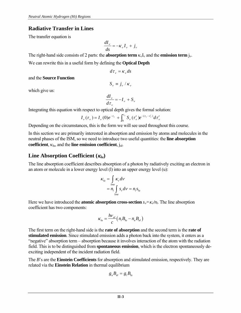
Radiative Transfer in Lines

The transfer equation is

jI

ds

dI

The right-hand side consists of 2 parts: the absorption term I and the emission term j.

We can rewrite this in a useful form by defining the Optical Depth

dsd

and the Source Function

/jS

which give us:

SI

d

dI

Integrating this equation with respect to optical depth gives the formal solution:

deSeII )(

0)()0()(

Depending on the circumstances, this is the form we will see used throughout this course.

In this section we are primarily interested in absorption and emission by atoms and molecules in the neutral phases of the ISM, so we need to introduce two useful quantities: the line absorption coefficient, lu, and the line emission coefficient, jul.

Line Absorption Coefficient (lu)

The line absorption coefficient describes absorption of a photon by radiatively exciting an electron in an atom or molecule in a lower energy level (l) into an upper energy level (u):

lu

line

l l lu

line

d

n s d n s

Here we have introduced the atomic absorption cross-section s=/nl. The line absorption coefficient has two components:

ullu l lu u ul

hn B n B

c

The first term on the right-hand side is the rate of absorption and the second term is the rate of stimulated emission. Since stimulated emission adds a photon back into the system, it enters as a “negative” absorption term – absorption because it involves interaction of the atom with the radiation field. This is to be distinguished from spontaneous emission, which is the electron spontaneously de-exciting independent of the incident radiation field.

The B’s are the Einstein Coefficients for absorption and stimulated emission, respectively. They are related via the Einstein Relation in thermal equilibrium

u ul l lug B g B


II-4

The Einstein B coefficients can in turn be written in terms of the Einstein A Coefficient for spontaneous emission (rate of radiative de-excitation) by

3

38ul ulul

cB A

hp n=

where 2 2 2

3

8ul ul

e

eA f

m c

p n=

here ful is the emission oscillator strength of the transition which is related to the absorption oscillator strength via the statistical weights of the levels:

u ul l lug f g f=

By convention there is no Alu term.

This gives us an equation for the atomic absorption cross-section:

1

ul ulu lu ul

l lline line

ul u llu

l u

h ns s d d B B

n c n

h n gB

c n g

nn

nkn n

n

æ ö÷ç ÷= = = -ç ÷ç ÷çè ø

æ ö÷ç ÷= -ç ÷ç ÷çè ø

ò ò

Recall from Chapter I that the departure coefficients relate the true level populations (n) to the LTE level populations (n*) via

*l l ln b n

and the LTE level populations are related via the Boltzmann Equation:

*/

*ulE kTu u

l l

n ge

n g

Putting all the pieces together gives:

/1 ulh kTulu abs

l

bs s e

bn-

æ ö÷ç ÷= -ç ÷ç ÷çè ø

Where we have defined the integrated atomic absorption cross-section, sabs, to be:

2ul

abs lu lue

h es B f

c m c

n pº =

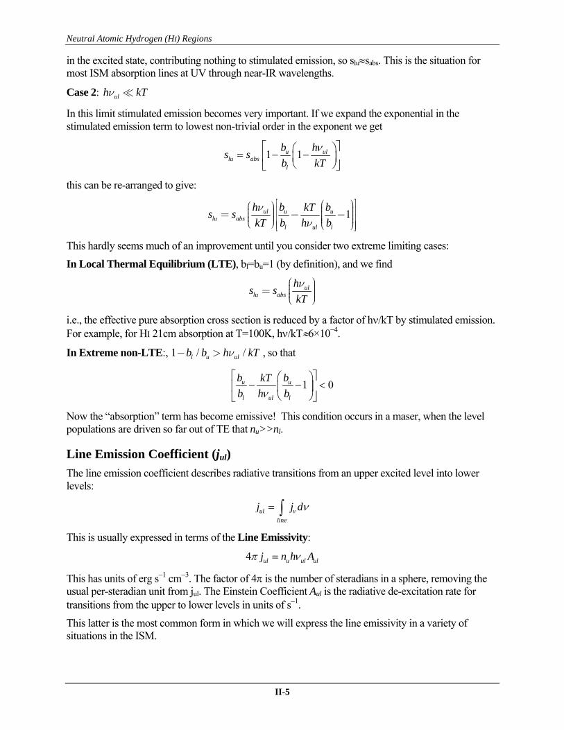
Written this way, slu is just the integrated atomic absorption cross-section modified by a stimulated emission correction expressed in terms of the departure coefficients and an exponential in hv/kT, where T is the kinetic temperature of the system. The limiting behaviors are instructive:

Case 1: ulh kTn

In this limit the stimulated emission term vanishes and the line formation is dominated by pure absorption. Since in the ISM we expect most species to be in the ground state, very few species will be


II-5

in the excited state, contributing nothing to stimulated emission, so slusabs. This is the situation for most ISM absorption lines at UV through near-IR wavelengths.

Case 2: ulh kTn

In this limit stimulated emission becomes very important. If we expand the exponential in the stimulated emission term to lowest non-trivial order in the exponent we get

1 1u ullu abs

l

b hs s

b kT

this can be re-arranged to give:

1ul u ulu abs

l ul l

h b bkTs s

kT b h b

nn

é ùæ öæ ö ÷ç÷ ê úç ÷= - -ç÷ç ÷÷ ê úçç ÷çè ø è øê úë û

This hardly seems much of an improvement until you consider two extreme limiting cases:

In Local Thermal Equilibrium (LTE), bl=bu=1 (by definition), and we find

ullu abs

hs s

kT

næ ö÷ç= ÷ç ÷çè ø

i.e., the effective pure absorption cross section is reduced by a factor of h/kT by stimulated emission. For example, for HI 21cm absorption at T=100K, h/kT6×10−4.

In Extreme non-LTE:, 1 / /l u ulb b h kTn- > , so that

1 0u u

l ul l

b bkT

b h b

Now the “absorption” term has become emissive! This condition occurs in a maser, when the level populations are driven so far out of TE that nu>>nl.

Line Emission Coefficient (jul)

The line emission coefficient describes radiative transitions from an upper excited level into lower levels:

ul

line

j j d

This is usually expressed in terms of the Line Emissivity:

4 ul u ul ulj n h A

This has units of erg s1 cm3. The factor of 4 is the number of steradians in a sphere, removing the usual per-steradian unit from jul. The Einstein Coefficient Aul is the radiative de-excitation rate for transitions from the upper to lower levels in units of s1.

This latter is the most common form in which we will express the line emissivity in a variety of situations in the ISM.


II-6

UV/Visible Absorption Line Formation

In Visible and UV interstellar absorption lines stimulated emission is unimportant because ulh kTn

for typical interstellar kinetic temperatures. These lines are therefore formed in the “pure absorption” limit, and the equation of radiative transfer has the simple solution:

,0I I e

Alternatively, we can express this in wavelength units; since UV and visible-light spectra are usually plotted in wavelengths (we’ll see frequency again in the radio regime):

,0I I e

Ideally, observation of an absorption-line profile can be turned into a measurement of the optical depth, , for the line species. In practice, however, effects of finite instrumental resolution compared to the actual line width, limits on signal-to-noise, and so forth are such that we need to express the line strength in terms of an integrated observable, the Equivalent Width, W, which is independent of spectral resolution:

,0

,0

I IW d

I

Equivalent widths have units of Å or mÅ in the UV and visible bands. In words:

The Equivalent Width of an absorption line is the width that a line would have if it had a rectangular profile with zero intensity at the line center.

The “area” of the line here is defined as the integrated area of the absorption profile measured from the local continuum level, I,0. Note the operative term here is “local”: equivalent widths are defined in terms of the unabsorbed continuum located immediately surrounding the absorption line of interest. In practice one does not normally measure the true “global” continuum shape of a spectrum, but instead estimates the local shape around the spectral features of interest. Note also that all information about the detailed line profile shape is lost in measuring an equivalent width (e.g., the line in the figure above is not symmetric).

In effect, this definition of the equivalent width “divides out” the spectrum of the background source. In practice, equivalent widths are measured by integrating the spectral line numerically after fitting a

I /I,

0

0

1

W


II-7

local “pseudo continuum” using adjacent unabsorbed regions of the spectrum. If the spectrum is very complex (may stellar and/or interstellar absorption lines close to one another), defining this local continuum can be problematical. In general, uncertainty in how to measure the local continuum is the principal source of systematic error in measuring equivalent widths.

The equivalent width is an extremely useful quantity because what matters is the fraction of the light absorbed, not the total count of the photons absorbed, by the intervening material. By dividing out the spectrum of the background source, we have normalized the absorption-line profile. The equivalent width, then, measures the effective area of this normalized absorption-line, integrating over the detailed line profile shape. As a result, two stars with very different apparent brightnesses and intrinsic spectra, viewed along the same line-of-sight and path length through and the same interstellar cloud, will yield the same equivalent widths. In many cases, we will find that relative quantities are more useful to us than absolute measurements.

The Equivalent Width Curve of Growth

A traditional method of analyzing absorption line data is via the Curve of Growth.

Consider an atom at rest. The absorption coefficient, , for a lower-to-upper transition will be:

4

2 2 208 ( )

o u uul

l u

gA

c g

The term in []’s is the Lorentzian or “Damping Profile” that characterizes the natural broadening of the line due to quantum mechanical uncertainty. The damping width is characterized by the radiation damping width, u, for the upper state is defined as the sum of all allowed downward radiative transitions out of that state:

20

4u uii u

Ac

The units of u are typically given in Angstroms or microns as appropriate to the transition being considered. Each upper level has a different damping width.

An interstellar cloud is an ensemble of atoms all moving about with some combination of thermal and non-thermal motions (e.g., turbulence, bulk flows, etc.). The natural absorption-line profile is therefore Doppler broadened by the combination of all of these motions along the line of sight to the observer. The distribution of line-of-sight velocities is (y), such that

1)( dyy

Here y is the dimensionless velocity parameter, y=v/b, the ratio of the line-of-sight velocity to the internal velocity dispersion, b. For a Maxwellian distribution of velocities in 3-space, the velocities project onto the line of sight with a Gaussian distribution:

21)( yey

For purely thermal motions with kinetic temperature T the Doppler Velocity Dispersion is:

2/12

m

kTb


II-8

Adding random turbulent velocities with a characteristic velocity dispersion of 2turb gives

2/122

turbm

kTb

[NOTE: be careful not to confuse the dimensionless “bj” departure coefficient with “b” the Doppler velocity dispersion. Sadly there are only 26 letters in the alphabet and so there has been considerable re-use – the key to survival in reading the ISM literature is to be careful of carrying forward definitions from one ISM phase to another and keeping aware of the context. The aggregation of a century of nomenclature doesn’t make it easy.]

The effect of the non-zero line-of-sight velocity of an individual atom is to Doppler shift the natural profile’s line center from 0 to (1+v/c)0. The resulting optical depth, , for the ensemble of atoms is the average of the individual ’s over (y), hence:

( ) ( )lN y y dy

Here Nl is the column density of atoms with electrons populating the lower state out of which we observe an absorption line:

( )L

l loN n s ds

This integral is taken along the line of sight (s) between the observer and the background source (e.g., a star) at distance L. Writing this out in full detail:

402 2 2

0

( )8 [ (1 / )]

u ul ul

l u

gN A y dy

c g cl

l gt y

p g l l

+¥

-¥

=+ - +ò v

This is rather complex, but we can simplify it by introducing four parameters:

0

0

/

( - )

/u

y bb

bc

ub

a b

v

These are the dimensionless velocity parameter, y, defined as before; the velocity dispersion, b, rewritten in units of wavelength, b; a dimensionless Doppler parameter, u, and the ratio of the natural (damping) width to the Doppler width, a. Substituting these definitions and assuming a Gaussian line-of-sight velocity distribution gives:

2403/2 2 28 ( )

yu ul

ll

g A a eN dy

c g b a u y

The first term in []’s above is the optical depth at line center, 0:

40

0 3/28u ul

ll

g AN

c g b

The second term in []s is the Hjerting Function, the convolution of the Lorentzian damping profile convolved with the Gaussian line-of-sight velocity distribution:


II-9

dy

yua

eauaH

y

22 )(),(

2

The Hjerting function has no analytic solutions, and it is usually evaluated by numerical integration. We can, however, gain some useful insights by making a power-series expansion of H(a,u) in a:

)()()(),( 10 uHauaHuHuaH nn

The first two terms are:

21

01

)(

)(2

uuH

euH u

H0(u) is a Gaussian profile describing the line core. H1(u) is the first “damping term” that describes the growth of the line wings (aka the “damping wings”) as the optical depth increases.

Recall that the equivalent width, W, of the line is defined as:

,0

,0

I IW d

I

For pure absorption ,0I I e

this becomes

deW 1

Substituting in the optical depth in terms of the Hjerting Function, we get the useful general form:

0 ( , )1 H a uW b e dutl l

-= -ò

where this integral is evaluated over the line-of-sight velocities rather than over wavelength.

What we measure is W, but what we want to derive is the optical depth with wavelength, , which in turn measures how much of the given species is producing the absorption we see along the line of sight. This conversion is described by the Equivalent Width Curve of Growth.

There are two limiting cases of interest that describe the properties of the Curve of Growth:

Case 1: The natural width u is much smaller than the Doppler width, b (a = u/b 103).

If the optical depth at line center, 0, is relatively small (<103), then only the first term in the Hjerting function is important:

2

),( ueuaH In this case the line profile is the Doppler (Gaussian) core with no significant contribution from the damping wings. There are two regimes of interest:

a) Optically Thin ( 0 1t ):

In this case, we can expand e to lowest non-trivial order in :

dueb

ddeW

u 2

0

1


II-10

Evaluating the integral, and dividing by the Doppler width, b, leads to:

0

b

W

In this case the equivalent width (in dimensionless units of the Doppler width) grows linearly with optical depth 0. We call this the Linear Part of the Curve of Growth.

b) Optically Thick, but 30 10t < :

The lines are optically thick, but not so optically thick (in the limit a<103) that the damping wings become important. In this case, we have:

dueb

W ue2

01

This equation is not analytically integrable, but the limiting behavior is

large for 0

)saturates"" core (line small for 11

2

0

u

ue

ue

The turnover point occurs when

00

200

0

ln0ln

:lyequivalentor ,120

uu

e u

Hence

00 ln22

ub

W

In this regime the equivalent width of the line grows very slowly even with large changes in the optical depth. We call this the Flat Part of the Curve of Growth.

Case 2: Large optical depth 0 and large column density Nl

In this case, we can no longer ignore contributions from the damping terms in H(a,u). For example, HI Lyman series lines, like Ly, have a103 but it is very abundant so that the column density is very high. In this case

200

2

),(u

aeuaH u

The damping wings become important when

2

2

ueu

a

For Ly, damping becomes important for u29.8 by this criterion.

Because the line core has become “saturated”, all subsequent “growth” of the line equivalent width will be due to the increasing contributions from the unsaturated line wings far from line center, hence:


II-11

20u

a

The equivalent width is then:

duedueb

W uau )1()1(2

0 /)(

Rewriting this by setting 20

2 / uax gives:

x

x dea

b

W1

2/1

0 )1(2

This is analytically integrable, hence

2/1

02

a

b

W

Here the equivalent width of the line grows like the square root of the optical depth and we say we are on the Square-Root part of the Curve of Growth.

These three regimes describe the behavior of the Equivalent Width Curve of Growth. At the transition regions, we of course need to evaluate the integrals numerically. A Curve of Growth computed numerically for interstellar HI Ly is shown in the figure below, illustrating the three regions (linear, flat, and square root) derived above. In addition, we show spectra of the interstellar NaI D lines that exhibit the range of behaviors.

The most useful measurements occur at the extremes of the curve in the linear and square root parts of the curve. In the flat part, between the onset of saturation of the line core and the onset of significant growth of the damping wings, large changes in optical depth lead to very small changes in the measured equivalent width. Thus nearly saturated but undamped lines provide little useful data on the line-of-sight column densities.

Equivalent Width Curve of Growth for HI Ly, showing the main regions derived in the text


II-12

Interstellar NaI-D absorption lines from Welty et al. [1994, ApJ, 436, 152]. These profiles show a mix of linear ( Cyg), flat ( Per & Ori), and square-root ( Oph) absorption lines.

Practical Considerations: In practice, curve of growth methods are quite powerful, as they can relate the product Nf to a direct observable, W, that is relatively insensitive to the choice of spectral resolution or fine details of the spectroscopic experiment. In principle, two different spectrometers working at very different resolutions and on different telescopes with different detectors should be able to measure the same equivalent widths to within the irreducible measurement uncertainties. However, because the equivalent width integrates over the detailed line profile shape, we do lose some information that might be useful.

Real interstellar absorption lines are often highly structured with a mixture of both saturated and unsaturated components because the line of sight to a particular star will often intersect a number of interstellar clouds with a wide range of column densities. While technically the equivalent width is insensitive to the spectral resolution (modulo effects of signal to noise which affects mainly the contrast of the line against the continuum), at lower spectral resolutions the saturated and unsaturated components will be blended, making interpretation of the composite line’s equivalent width in terms of a single column density problematic at best.


II-13

In the case where lines are heavily saturated or show measurable damping wings (e.g., damped HI Lyman absorption systems), the equivalent width curve of growth method is unreliable. One cannot tell where the continuum should be placed, which leads to large systematic errors in measuring W. In this case, various alternative methods have been used, for example the “Continuum Reconstruction Method” described by Bohlin et al. (1975, ApJ, 200, 402).

At very high spectral resolutions (R>104), an alternative is to use the observed line profile and fit models to account for instrumental effects and the contributions from multiple absorption components with different column densities. The problem here is a lack of a complete database of UV spectra with sufficient resolution to employ these methods. One usually has to fall back on making assumptions about the intrinsic line profile shape.

The intermediate case occurs when the lines are fully resolved (i.e., when the line width is larger than 23 instrumental widths), but not necessarily resolved into fine velocity structure, a particularly powerful class of techniques has emerged to deal with these data. These techniques use direct integration of the observed optical depth profiles. Such methods make no a priori assumptions about either the detailed line shapes or the velocity distribution of the gas (unlike the case with the curve of growth, continuum reconstruction, and line profile modeling approaches).

A particularly good example of this type of analysis is the “Apparent Optical Depth Method” described by Savage & Sembach (1991 ApJ, 379, 245). This method does an excellent job of allowing discrimination of saturated structures in velocity space. When many different species are present in a spectrum, it provides a complete N(v) profile by letting the different unsaturated parts fill in the gaps left by saturated species. This method provides a modern alternative to the traditional Curve of Growth analysis, and has been used in a number of recent absorption-line studies of the ISM.

Despite the practical caveats, the curve of growth still permits us to address a number of problems quantitatively in a way that illuminates what can be learned from IS absorption lines. The new methods lend us a greater degree of measurement precision, but no additional basic physical insight.

Applications of Interstellar Absorption Lines

1) Interstellar Ly

The HI Lyman series lines are UV resonance lines that arise in radiative excitations out of the n=1 ground state of HI. First seen in the ISM in the early 1970s with the launch of the first UV satellites, they are seen along every line of sight, from early-type stars to late-type stars with chromospheric activity (you need some UV flux to observe them).

The optical depth of the HI Lyman series is very high, and on the damping (square-root) part of the Curve of Growth for most interstellar clouds, hence:

22/1

0

a

b

W

The optical depth at line center, 0, is given by

40

0 3/28u ul

ll

g AN

c g b

From this result and the definition a=u/b, the Doppler width, b, cancels out, and we can write the equivalent width of the line as a function of the column density, Nl alone:


II-14

1/240

2u

l ul ul

gW N A

c gl

lg

p

æ ö÷ç ÷=ç ÷ç ÷çè ø

The u’s are computed by summing over all the A’s for the downward transitions out of the upper excited state of the particular absorption line of interest. For Ly, which is the 2p1s line, there is only 1 term in the computation of 2p (only one place for the electron to go, back to 1s). For Ly (3p1s) there are two terms (3p1s and 3p2s are possible radiative decay channels), and so forth.

Putting in numbers for Ly, we can solve for the column density along the line of sight as a function of the equivalent width:

)(cm 10867.1 -2218 WN Ly

for W in units of Angstroms. Observations of stars at d100pc give W(Ly)10Å, which implies a column density of Ly absorbers of NLy1.91020 cm2. A line of sight of 100pc31020 cm implies a mean hydrogen column density of nH0.6 cm3. For nearby stars, however, nH0.1 cm3 or less is typical, indicating that we reside in a “local bubble” characterized by a lower average density.

We can also estimate the mean abundance of Deuterium in the ISM by measuring the Lyman-series absorptions from DI. The DI Lyman lines are shifted blueward of their respective HI counterparts by a small isotopic shift due to the neutron in the nucleus (the Rydberg constant is proportional to the reduced mass of the nucleus). The table below gives the isotopic shifts for the first 3 Lyman series lines of HI and DI:

HI DI

Ly 1215.67Å 1215.34Å 0.33Å Ly 1025.72Å 1025.44Å 0.28Å Ly 972.54Å 972.27Å 0.27Å

Since HI Ly is so strongly saturated in the ISM, with very strong damping wings (W10Å), the DI line is lost in the saturated HI line core. You therefore need to measure the DI lines associated with higher-order HI Lyman lines, like Ly, Ly, etc., that have less strongly damped lines. For example, measurements of HI and DI absorption along the line of sight to Centauri (where there is no detected H2 absorption), one measures D/H(1.40.2)105, smaller than 2104 measured on Earth from the

Interstellar DI and HI Ly absorption lines towards the white dwarf star WD0621-376 observed with FUSE. From Lehner et al. (2002, ApJS, 140, 81).


II-15

3/2 1/2

3/2 5/2

2D

1334.5Å 1335.7Å

158m 2Po

solar wind or ocean water. You can also measure HD molecular absorption bands (the analog of the H2 Lyman bands), but it is hard to convert from HD/H2 to D/H.

The Copernicus satellite (mid 1970s) was the first UV satellite that was sensitive to the higher-order Lyman series lines in the Far-UV (most UV satellites, except EUVE, were not sensitive below about 1100Å). Subsequent Far-UV studies have relied on either sounding rockets or short-duration space missions (e.g., ORFEUS-SPAS I and II, or IMAPS on the Shuttle). Lyman/FUSE (launched June 1999) is the first long-duration satellite mission since the Copernicus satellite 1970s to work in this Far-UV region (and is ~105 times more sensitive). So far, it has provided a number of good measurements of D/H in the local ISM from HI and DI Lyman series lines out to distances of 100pc from the Sun (and a few sight lines out to ~1kpc with IMAPS). The data show a pretty constant D/H1.21.7×105, with the dispersion in values increasing with distance from the Sun.

2) ISM Gas-Phase Abundances

So many different species produce UV absorption lines in the ISM, from Hydrogen to rare metals, that we can get a pretty clear picture of the relative gas-phase abundances of the various elements from UV absorption-line studies. Among the scientific questions these permit us to address are chemical evolution of the ISM (in particular the mix of elements from different nuclear processes like -process, neutron capture and proton capture) and the depletion of refractory elements onto dust grains.

The current status of UV absorption-line abundances, especially as learned from the Hubble Space Telescope GHRS, has been reviewed by Savage & Sembach (1996, ARAA, 34, 279). A table of measured sight lines and the elements seen along them is reproduced on the following pages. The lines of sight to 2 stars, Ophiuchus and Persei, are particularly rich in interstellar absorption lines. These sight lines cross through regions of high column density, and many rare metal species (Cu, Zn, etc.) are very well studied there. Examples of spectra along the Oph sight line are reproduced on the next page. Other sight lines have at least 5 or more different atomic species available for study.

A particular achievement of GHRS, which flew from 19901996, was the detection of unsaturated CII absorption (e.g., CII]2325Å absorption). In previous studies, only one line of sight, towards Scorpii, had unsaturated CII lines, the rest were all on the flat part of the curve of growth and produced no useful information (limits only). As a result, GHRS has permitted the first definitive interstellar gas-phase carbon abundances.

A particularly important result of the HST/GHRS data has been to greatly refine measurements of the depletion of gas-phase elements onto dust grains for sight lines that pass through both warm and cold phases of the ISM in both the disk and the halo of the galaxy. We will treat this subject in more detail later in the course when we discuss the properties of dust grains.

3) Thermal Balance

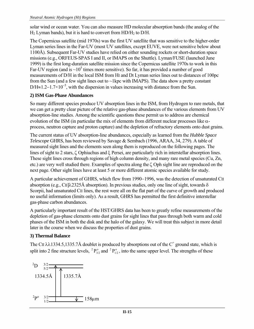
The CII 1334.5,1335.7Å doublet is produced by absorptions out of the C+ ground state, which is split into 2 fine structure levels, o

3/22 P and o

1/22 P , into the same upper level. The strengths of these


II-16

absorption lines give the relative populations in each of these levels. This is of particular interest as transitions within this fine structure ground state are responsible for producing the [CII]158m emission line. Morton’s 1975 observations of the CII 1334.5Å and 1335.7Å ratio showed a significant population of atoms in the o

3/22 P state (the upper most of the fine structure level). This

suggested that [CII]158m line could be a strong cooling line in HI regions. It was not until the 1980s that the Kuiper Airborne Observatory detected Far-IR [CII] emission from the ISM, as predicted by Morton.


II-17

The HI Hyperfine Structure Line Most of our knowledge of the distribution of neutral atomic hydrogen in the ISM of the Milky Way and other galaxies come from observations of the strong 21-cm line. This line arises from transitions between the hyperfine structure levels in the ground state of Hydrogen, and is seen in both emission and absorption. This section reviews the physics of the HI hyperfine transition and of HI 21-cm line formation in both absorption and emission.

Hyperfine Splitting of HI: A little light quantum mechanics.

The 1s2S1/2 ground state of HI is split by the interaction between the magnetic moments of the proton and electron spins.

The electron magnetic moment is:

Jg Bee

where:

B

electron Lande factor 2.00232

Bohr Magneton 2

electron quantum number

e

e

ge

m cJ L S

The proton magnetic moment is:

Ig NNp

where:

N

proton Lande factor 5.58 (experimentally)

Nuclear Magneton 2

proton quantum number, 1/ 2

N

p

ge

m cI I

A way to think of the Landé factors are that they express the difference between the classical and quantum descriptions of the magnetic moment of a sphere of uniform mass and charge density. The different Landé factors reflect the fact that the electron is a single particle with charge 1, but the proton is a combination of 3 quarks with fractional charges that add up to +1. The quantization of the coupling of the ’s results in the HI ground state being split into two states corresponding to parallel and anti-parallel spins of the electron and proton. The difference in energy, W, between the ground state and the hyperfine levels is given by:

e pW

Following Condon & Shortly, for the 2S1/2 terms, this is exactly

I

IW pe

1,1

3

8

For HI, with I=1/2, this becomes

3,13

8 peW


II-18

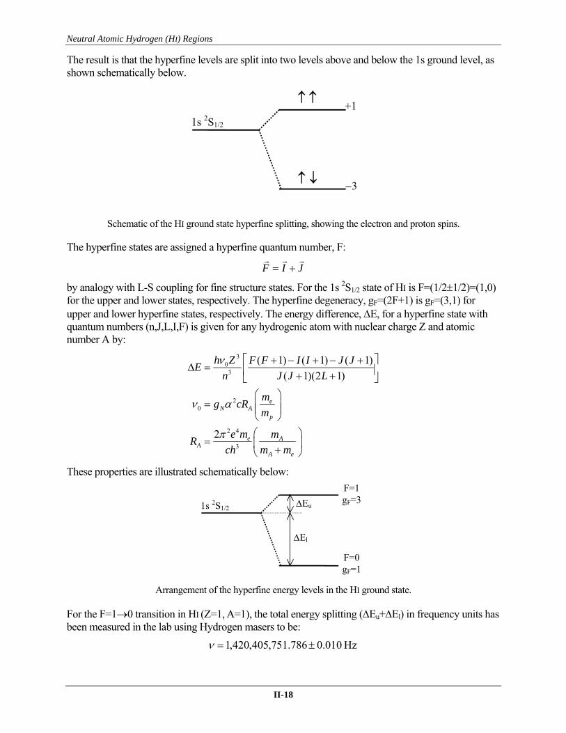
The result is that the hyperfine levels are split into two levels above and below the 1s ground level, as shown schematically below.

1s 2S1/2

+1

3

Schematic of the HI ground state hyperfine splitting, showing the electron and proton spins.

The hyperfine states are assigned a hyperfine quantum number, F:

JIF

by analogy with L-S coupling for fine structure states. For the 1s 2S1/2 state of HI is F=(1/21/2)=(1,0) for the upper and lower states, respectively. The hyperfine degeneracy, gF=(2F+1) is gF=(3,1) for upper and lower hyperfine states, respectively. The energy difference, E, for a hyperfine state with quantum numbers (n,J,L,I,F) is given for any hydrogenic atom with nuclear charge Z and atomic number A by:

30

3

20

2 4

3

( 1) ( 1) ( 1)

( 1)(2 1)

2

eN A

p

e AA

A e

h Z F F I I J JE

n J J L

mg cR

m

e m mR

ch m m

These properties are illustrated schematically below:

1s 2S1/2

F=1gF=3

F=0gF=1

Eu

El

Arrangement of the hyperfine energy levels in the HI ground state.

For the F=10 transition in HI (Z=1, A=1), the total energy splitting (Eu+El) in frequency units has been measured in the lab using Hydrogen masers to be:

Hz 010.0786.751,405,420,1


II-19

This is one of the few times you can quote a number in astrophysics to that kind of precision! In more convenient frequency and wavelength units, however:

cm 106.21

MHz 4.1420

The F=10 transition is a magnetic dipole transition, with transition probability

1-15

2

101

322

22

10

s 1085.2

12

11

3

4

M

Fcm

heA

e

This relatively low transition probability gives a mean lifetime of the state of 1.1107 years. The natural width of this transition is

Hz 105.42

161010

A

Compared to the thermal Doppler width expected from an ensemble of HI atoms with kinetic temperature of 100K:

Hz 47003

20 mc

kTth

For most astrophysical conditions, we expect the width of the HI 21cm line (either in emission or absorption) to be dominated by the Doppler width due to thermal and/or turbulent motions.

Level Populations

We expect the level populations in the HI hyperfine levels to be far from LTE in most cases. As a starting point, the LTE populations are given by:

kTheg

g

n

n /

0

1

*0

*1

where “1” and “0” refer to the hyperfine quantum number, F, of the states, T is the kinetic temperature of the HI cloud, and is the frequency of the hyperfine transition. The non-LTE level populations are expressed in terms of an excitation temperature, TS, which is traditionally called the “Spin Temperature” of the system:

SkTheg

g

n

n /

0

1

0

1

Putting in the values of the g’s, and using / 68 mKh kn = , the transition energy in units of Kelvin:

0.068/1

0

3 STne

n-=

For most astrophysically interesting conditions, TS68mK, and so we have to rely on subtle absorption effects in the line formation physics which, as we shall see, are very sensitive to small deviations in n1/n0.


II-20

Optical Depth

In general, as we saw previously, the optical depth in a transition is given by

dyA

g

g

cyN

20

210

1010

0

1

2

40

0)(8

)(

where

)/1(00 cv

Integrating over wavelength gives the integrated line optical depth commonly used in radio astronomy 40 1

0 1000 8

gd N A

c g

This equation relates total HI absorption to the column density of HI along the line of sight, N0.

Just to be sure of confusing everything, the traditional way of writing this in radio astronomy is to recast the distribution of velocities, (y), in frequency units:

dfdyy )()(

and so we can write the optical depth at a particular wavelength, , as

d

dfA

g

g

cN )(

8 100

140

0

since d/d=c/2 (eliminate the sign by integrating backwards) we can write:

)(8

310

20

0

fAN

or, finally purging the mixed wavelength/frequency units in favor of frequencies:

)(8

3102

2

0

fAc

N

where in all of the equations above, N0 is the column density of HI in the F=0 (unexcited) hyperfine state. The gF degeneracy values (3 and 1, respective for F=1,0) tell us that the mix of states in thermal equilibrium should be (modulo a TS correction <<1):

HI

HI

NN

NN

4

34

1

1

0

So that:

)(32

3102

2

fANc

HI

This is the form of the HI 21cm optical depth most often used by radio astronomers.


II-21

Stimulated Emission

The calculation of the optical depth in the previous section was assuming the pure absorption case. However, while stimulated emission is insignificant at UV, optical, and near-IR wavelengths, it is very important at radio, mm, and (sometimes) far-IR wavelengths.

The effect of stimulated emission is for the radiation field to induce downward transitions from the upper excited states at a rate proportional to the local density of photons. This adds photons in the direction of the radiation field, making these photons coherent.

F=1

F=0

Schematic of Stimulated Emission

The intensity of the stimulated emission component, ISE, is proportional to the intensity of the local radiation field:

IBnIBnI uluSE 101

The absorption component is also proportional to the local radiation field:

IBnIBn lul 010

The B’s are related via the statistical weights:

u ul l lug B g B

So that, the net upward transitions (pure absorption out of F=0 less stimulated emission out of F=1 to F=0) is thus:

1

0

0

1010

011

01010

1g

g

n

nIBn

IBg

gnBn

Recall that the relative non-LTE level populations, n1/n0, were written in terms of the spin temperature, TS, as a Boltzmann-like equation

SkTheg

g

n

n /

0

1

0

1

hence

SkThe /1

Recall now that h/k=68 mK << TS, so expanding the exponential to lowest non-trivial order gives:

SkT

h


II-22

To account for stimulated emission, we must multiply the optical depth derived in the pure-absorption case (above) by a correction factor h/kTS, hence:

los S

HI

S

HI

dsT

fn

fAkT

Nhc

)(1095.7

)(32

3

3

100

2

Here I’ve substituted the definition of the column density of HI, NHI, in terms of the integral of the HI density, nHI, along the line of sight

los

HIHI dsnN

and put in the values of the physical constants, nHI is in units of cm3, TS is in K, and ds is in parsecs. Note that in general the HI density, spin temperature, and distribution of cloud velocities f() are all functions of position, s, along the line of sight.

21-cm Line Formation

HI 21-cm Emission Lines

The equation of radiative transfer is

;dI j

Id

d ds

n nn

n n

n n

t kt k

=- +

=

which has the solution:

( )

0

0

;

( ) ( )

s

s

I j e ds

s s ds

In radio astronomy, it is conventional to express the observed intensities in units of a Brightness Temperature, ( )BT n , because at =21 cm, we are in the Rayleigh-Jeans limit:

2

2

2( )B

kI T

cnn

n=

The radiation is not really blackbody, but the R-J limit allows us to express any I in terms of an equivalent temperature for a blackbody that would give the same intensity. Brightness temperatures are actually what radio astronomers measure in their receivers at radio wavelengths, unlike the case in UV, visible, and IR wavelengths where (ideally) we count incident photons.

The emission coefficient expressed in temperature units (K/cm), J, is given by

j

k

cJ

2

2

2


II-23

Kirchoff’s Laws relate and J through the spin temperature, TS by:

STJ

Multiplying the transfer equation by a factor of c2/2k2, and re-arranging gives:

)(

BSB TT

d

dT

for the Rayleigh-Jeans limit. This equation has the solution:

( )

0

( ) sB S

S

T T e ds

T e d

where

0

( ) ( )s

s s ds

Thus is the optical depth to infinity along the line of sight, while is the optical depth to distance s along the line of sight.

Assuming that TS is constant along the line of sight (i.e., that we have an isolated isothermal cloud), the solution of the radiative transfer equation reduced to

eTT SB 1)(

In general, however, both TS and will be expected to vary with position, and solutions of the full transfer equation are required (they are not pretty).

Recall from our earlier discussion of UV and visible lines that in the limit h<<kT, we found

l lu l absexc

hn s n s

kT

where sabs is the integrated atomic absorption cross-section for the transition. In this limit, the absorption is nearly completely compensated for by stimulated emission out of the excited state, so that the effective absorption coefficient depends on small variations of n1/n0 with spin (excitation) temperature, TS. Numerically (from Kerr 1968 in Ch 10 of Middlehurst & Aller):

TS (K) n1/n0

10 2.9806 100 2.9981 1000 2.9998

These numbers show that as the spin temperature rises, the ratio of the hyperfine level populations approaches the ratio of the statistical weights (3.00). For the purposes of deriving column densities from HI line measurements, this means that assuming n1/n0=3 is a reasonable approximation.


II-24

Writing in terms of the transition probability A10:

)(8 0

1102

2

0

fkT

h

g

gA

cn

S

Since nHI=4n0, the optical depth is:

21

10200

( )4 8

sHI

S

N gc hds A f

g kT

NHI is the HI column density. Putting in the numbers for the HI 21-cm transition:

)(1059.2 15 fT

N

S

HI

Solving for NHI:

14 -23.88 10 ( ) cmHI SN T g d

(the function g() is the 1/f(), but both are arbitrary placeholders for “line profile” in different units, so the notation can be similarly arbitrary). Since emission lines are often observed in frequency bins or “channels”, radio astronomers will often derive the column density in a particular frequency bin:

-217 cm 1088.3)( KHzSHI TN

Alternatively, one often sees the column density measured in a particular radial velocity bin: -218 cm )(1082.1)( kmsSHI TN vvv

Here (v) is the optical depth in the radial velocity interval [v,v+dv].

To measure the column density of HI along the line of sight, we need to measure TS and , but the only observable is ( )BT n . To see how optical depths, and hence column densities, are measured in

practice, it is useful to examine two limiting cases:

Case 1: Optically Thin Limit, (v)<<1

In this case,

vv SB TT )(

so that bins km/sec 1in )(1082.1)( 18 vv BHI TN

or

line

BHI dTtotN vv)(1082.1)( 18

where the integral is often written as the “line intensity” expressed in units of “K km s1” (the somewhat odd unit you will find in many HI radio observation papers, especially older papers). Most extragalactic observations of the total HI content of galaxies determined from integrated 21-cm line measurements assume the optically thin case, and this is justified except for edge-on galaxies viewed in their mid-plane or large gas-rich merger remnants where lines of sight through the thickest parts of the galaxy are optically thick. It is also true of many, but not all, sightlines


II-25

through the disk of our own Galaxy – the exception being sight lines within a few degrees of the Galactic Center which are all optically thick.

Case 2: Optically Thick Limit, (v)>>1

In this case

SB TT

This happens because 21-cm photons emitted inside the cloud are absorbed within the cloud, and only those photons emitted from within 1 optical depth of the cloud surface escape. In this case the observed TB is independent of column density, and depends on TS. The column density must therefore becomes:

181.82 10 ( )HI SN T d

v v

where now we must integrate the optical depth over velocity instead of integrating over the observed emission-line profile in brightness temperature.

Line Broadening

Because the natural width, 10 is so small, Doppler broadening will dominate the line profile. This broadening takes two forms:

Thermal Broadening within a single cloud:

HD m

kT22

in which case the optical depth profile will be: 2

0 )/(0)( De

Bulk Motions of individual clouds:

i

iiDe

2,0 )/(

,0)(

Here the D,i are the thermal Doppler widths of the individual clouds.

In practice, we often add an arbitrary turbulent velocity term in quadrature with the thermal term to specify the line width, much like what is done at UV and visible wavelengths with interstellar absorption lines.

The narrowest HI 21cm absorption lines seen in the Galaxy are roughly Gaussian in shape, but most emission lines are decidedly non-Gaussian, appearing as a superposition of many blended Gaussian components.

HI 21-cm Absorption Lines

Consider a background radio continuum source (e.g., a quasar or radio galaxy) with a brightness temperature Tbg. The solution of the equation of radiative transfer in the R-J limit is thus:

0

( )B bg ST T e T e d

For a single, isothermal cloud, this reduces to

)()(

1)(

emissionabsorption

eTeTT SbgB


II-26

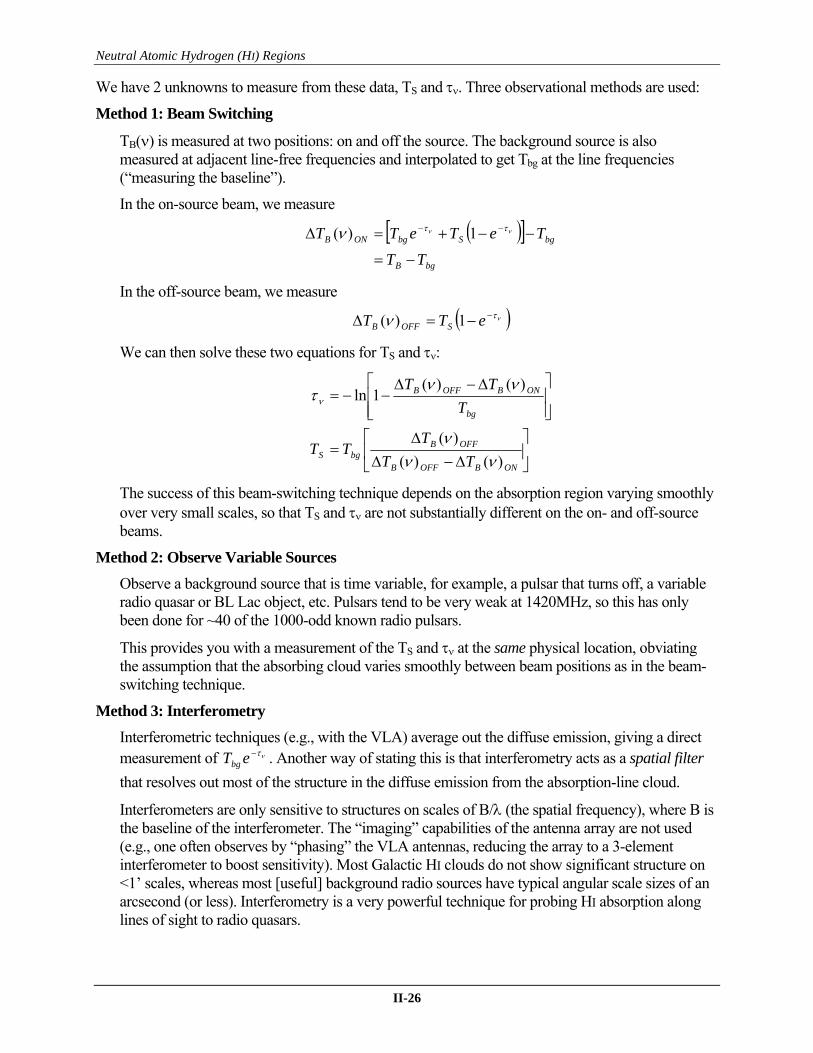
We have 2 unknowns to measure from these data, TS and . Three observational methods are used:

Method 1: Beam Switching

TB() is measured at two positions: on and off the source. The background source is also measured at adjacent line-free frequencies and interpolated to get Tbg at the line frequencies (“measuring the baseline”).

In the on-source beam, we measure

bgB

bgSbgONB

TT

TeTeTT

1)(

In the off-source beam, we measure

eTT SOFFB 1)(

We can then solve these two equations for TS and :

ONBOFFB

OFFBbgS

bg

ONBOFFB

TT

TTT

T

TT

)()(

)(

)()(1ln

The success of this beam-switching technique depends on the absorption region varying smoothly over very small scales, so that TS and are not substantially different on the on- and off-source beams.

Method 2: Observe Variable Sources

Observe a background source that is time variable, for example, a pulsar that turns off, a variable radio quasar or BL Lac object, etc. Pulsars tend to be very weak at 1420MHz, so this has only been done for ~40 of the 1000-odd known radio pulsars.

This provides you with a measurement of the TS and at the same physical location, obviating the assumption that the absorbing cloud varies smoothly between beam positions as in the beam-switching technique.

Method 3: Interferometry

Interferometric techniques (e.g., with the VLA) average out the diffuse emission, giving a direct measurement of eTbg . Another way of stating this is that interferometry acts as a spatial filter

that resolves out most of the structure in the diffuse emission from the absorption-line cloud.

Interferometers are only sensitive to structures on scales of B/ (the spatial frequency), where B is the baseline of the interferometer. The “imaging” capabilities of the antenna array are not used (e.g., one often observes by “phasing” the VLA antennas, reducing the array to a 3-element interferometer to boost sensitivity). Most Galactic HI clouds do not show significant structure on <1’ scales, whereas most [useful] background radio sources have typical angular scale sizes of an arcsecond (or less). Interferometry is a very powerful technique for probing HI absorption along lines of sight to radio quasars.


II-27

HI 21cm emission and absorption profiles towards 8 extragalactic radio sources from Radhakrishnan et al. (1972, ApJS, 24, 15). The dashed lines are fits to an optically thin emission-line component without a corresponding absorption component. The vertical lines delineate the velocity limits of the optically-thick absorption components. These are beam switching observations with the Parkes Telescope, so the vertical axis is TB(v). The narrow absorption lines correspond to discrete CNM clouds, and the broad optically-thin emission is diffuse WNM (intercloud) gas.

Excitation of 21-cm Emission

How do you excite HI into the excited hyperfine structure level?

The competing processes for determining the population of the upper excited hyperfine structure level are Collisional Excitation and Collisional De-excitation.

)1()0( FHXFHX

Because the lifetime of the excited state is so long (t01.1107 years), radiative de-excitations are relatively rare. Collisions with other HI atoms and electrons dominate.

The cross-sections for collisional excitation/de-excitation are:

01 0

10 1

( ) : excitation, with threshold / 0.068 K( ) : de-excitation (no threshold)

Q h kQ

vv

n =

Energy conservation demands

m

h

hmm

2 :holdwith thres

,2

1

2

1 21

20

0v

vv

Note also that electrons have a much larger speed than H atoms by a factor of (mp/me)1/2 45.


II-28

The Principle of Detailed Balance

In LTE, any microscopic process is precisely balanced by its inverse, thus collisional excitation with rate

*0 0 0 01 0 0( ) ( )xn n f Q dv v v v

is precisely balanced by collisional de-excitations with rate *1 1 1 10 1 1( ) ( )xn n f Q dv v v v

Energy conservation demands that

1100 vvvv dd

so that the collisional equilibrium condition (no radiative processes) becomes:

)()()()( 1101*10010

*0 vvvv QfnQfn

For a Maxwellian velocity distribution

kTmef 2/2 2

)( vvv

which means that the equilibrium condition becomes

)()( 1102/2

1*1001

2/20

*0

21

20 vvvv vv QenQen kTmkTm

In LTE, the Boltzmann equation tells us

kTheg

g

n

n /

0

1

*0

*1

but now

kTmkTmkTh eee

mmh

2/2//

21

20

21

20

2

1

2

1

vv

vv

Thus the exponentials cancel, leaving us with the Milne Relation:

)()( 110211001

200 vvvv QgQg

Since h/k=68mK is small for typical kinetic temperatures T, v0v1, and we have:

)(3

1)( 0110 vv QQ

Electron Collisions

Electron collisions dominate the excitation balance in HI if the electron density, ne>0.03nH. eFHeFH )1()0(

There are two modes:

1. Spin-Flip Collisions due to the magnetic field of the passing electron flipping the spin of the bound electron. This has a very small cross-section and is thus rare.


II-29

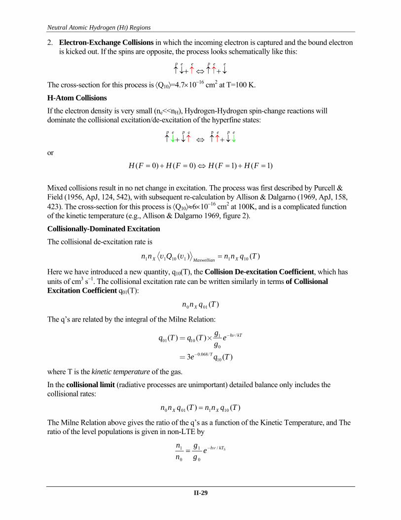
2. Electron-Exchange Collisions in which the incoming electron is captured and the bound electron is kicked out. If the spins are opposite, the process looks schematically like this:

p pe e e e

The cross-section for this process is Q10=4.71016 cm2 at T=100 K.

H-Atom Collisions

If the electron density is very small (ne<<nH), Hydrogen-Hydrogen spin-change reactions will dominate the collisional excitation/de-excitation of the hyperfine states:

pe

p p pe e e

or

)1()1()0()0( FHFHFHFH

Mixed collisions result in no net change in excitation. The process was first described by Purcell & Field (1956, ApJ, 124, 542), with subsequent re-calculation by Allison & Dalgarno (1969, ApJ, 158, 423). The cross-section for this process is Q1061016 cm2 at 100K, and is a complicated function of the kinetic temperature (e.g., Allison & Dalgarno 1969, figure 2).

Collisionally-Dominated Excitation

The collisional de-excitation rate is

)()( 10111011 TqnnQnn XMaxwellianX vv

Here we have introduced a new quantity, q10(T), the Collision De-excitation Coefficient, which has units of cm3 s1. The collisional excitation rate can be written similarly in terms of Collisional Excitation Coefficient q01(T):

)(010 Tqnn X

The q’s are related by the integral of the Milne Relation:

/101 10

0

0.068/10

( ) ( )

3 ( )

h kT

T

gq T q T e

g

e q T

n-

-

= ´

=

where T is the kinetic temperature of the gas.

In the collisional limit (radiative processes are unimportant) detailed balance only includes the collisional rates:

)()( 101010 TqnnTqnn XX

The Milne Relation above gives the ratio of the q’s as a function of the Kinetic Temperature, and The ratio of the level populations is given in non-LTE by

SkTheg

g

n

n /

0

1

0

1


II-30

where TS is the Spin Temperature1. Substituting both into the equation of detailed balance, we obtain the result

S kinT T

When collisions dominate the excitation, the Spin Temperature is driven to the Kinetic Temperature of the gas. In such circumstances we say that the level populations have “thermalized”.

Radiatively-Dominated Excitation

The opposite limit occurs at low densities when collisions are unimportant relative to radiative processes in the excitation equilibrium. In this case, the equation of detailed balance becomes

010101101 44 BnJBnJAn

where 4J is the radiation field density. With the HI 21-cm line we are in the Rayleigh-Jeans limit for most radiation fields, and so we can express the radiation-field density in terms of TR, the Color Temperature of the radiation field:

RkTc

hJ

3

2

From the Einstein Relations, the stimulated emission coefficient, B10 can be expressed in terms of the radiative transition probability, A10:

*

1010104T

TA

h

kTABJ RR

where

* / 68 mKT h k

Using the Einstein relation g0B01=g1B10 the equation of detailed balance in the radiation-dominated case becomes:

*100

10*101101 // TTA

g

gnTTAnAn RR

This can be solved for the ratio of the level populations:

*

*

0

1

/1

/3

TT

TT

n

n

R

R

Recalling that the non-LTE (“true”) level populations are given by:

*0.068/ /1

0

3 3S ST T Tne e

n

and given that we are in the limit that RT T* the relative populations reduce to

RT

T

n

n *

0

1 13

1 In keeping with the convention we established in Chapter I this should be called the "Excitation Temperature", but it is traditional to refer to it as "Spin Temperature" in radio astronomy. This is a recurrent theme we will encounter in ISM studies: each specialty has its own traditional nomenclature and notation that makes crossing between disciplines a challenge.


II-31

However, ST T* , so we also have from the Boltzmann equation

S

TT

T

Te

n

nS */

0

1 133 *

Thus RS TT , and in the radiation-dominated limit the spin temperature is driven to the color

temperature of the ambient radiation field by the effect of stimulated emission. Under typical astrophysical conditions, TR is the temperature of the cosmic microwave background (~2.725 K).

General Excitation

Reality lies between the two limits just discussed, and the excitation and de-excitation of the HI hyperfine levels are a mixture of collisional and radiative processes. If we assume for simplicity that only atomic collisions are important (ne0.03nH), the condition of detailed balance becomes:

)4()4( 010101010101 BJqnnBJAqnn HH

Following a procedure similar to the one used in the limiting cases discussed above, this equation can be solved for TS in the general case:

10

10 *

10

10 *

1 1

1

1

R

kin H R

S R

H

A TT n q T T

T A Tn q T

This form is somewhat more complicated than is usually found in most textbooks, but it has the virtue of emphasizing that the spin temperature is in effect a harmonic mean of the kinetic and radiation temperatures, with the radiation temperature weighted by a factor that includes the influence of stimulated emission and the relative importance of collisional vs. radiative de-excitation. The relative importance of collisional and radiative de-excitation can be parameterized in terms of a Critical Density, ncrit, at which the rates are roughly the same

10

10 ( )crit

An

q T .

When nH>ncrit, collisional de-excitation dominates and TSTkin, whereas in the low-density limit radiative processes dominate and TSTR as before. Because of the temperature dependence on q10, the critical density depends on temperature and does not have a simple analytic or even empirical power-law form (despite what you may find in some references). See for example the tabulation of Allison & Dalgarno. In general, the critical density is of order 10(45) cm3 for typical ISM conditions (T= few 100K).

The figure below shows a plot of TS/Tkin for Tkin=10 and 100K for the collisional rates tabulated by Allison & Dalgarno (1969). Note that TS does not exceed the background radiation temperature until well above the critical density. For most ISM conditions, this won’t be an issue as nH is nearly always much larger than ncrit, but this is not true at the very low densities of the intergalactic medium.


II-32

Plot of TS/Tkin for Tkin=10 and 100K.

Lyman- Pumping

In HI, absorption of Ly photons is almost immediately followed by re-emission (resonant scattering). This process, however, does not necessarily return the electron to the same hyperfine structure level as before absorption of the Ly photon.

Because most HI clouds are very optically thick to Ly photons, a single Ly photon is resonantly scattered many times before exiting the cloud. Field (1959, ApJ, 129, 551) showed that if the tiny energy difference of the hyperfine levels (6106eV compared to 10eV for Ly transition) is accounted for, a very slight slope in the center of the Ly line profile develops that will drive TSTkin.

Watson & Deguchi (1985, ApJL, 281, L5) have shown that in low-density extragalactic HI clouds this process can occur, and can lead to small changes in the observed TS that increases it compared to the expectations for the low-density limit.

In general, in the low-density limit (nHncrit) if no other radiation sources are present:

2.725 KS R CMBT T T

As other sources of TR come into play, nHncrit, both collisional processes and Ly pumping will start to drive TSTkin. In the Galaxy,

-3

-30.03 cm

0.1 1 cm100 K

e

H

kin

nn

T

»» -

»

Thus TSTkin is essentially always the case in HI regions in our Galaxy and other galaxies.


II-33

The CNM and WNM

HI 21cm studies of the Galaxy reveal that 21cm emission is virtually ubiquitous along every line of sight, but 21cm absorption is not. The typical N(HI)>51019 cm2, and the general run of emission lines are broader than the absorption lines (see the spectra from Radhakrishnan et al. above). This is taken as evidence for two physically distinct neutral thermal phases coexisting in the ISM:

Cold Neutral Medium (CNM), composed of cold (T<100K), dense (n=20–60cm3), clouds and filaments with a small filling factor (~1–4%).

Warm Neutral Medium (WNM), composed of diffuse, relatively low-density (~0.3cm3) gas with temperatures of ~5000K with a much larger filling factor (~30%).

Observations suggest that the CNM has a typical column density of 51019 cm2, with a median temperature of TS=58K, much colder than the canonical 100K. A column-density weighted average is ~70K, but some regions can be as cold as 15K and as warm as 250K. Detailed line profiles show that the CNM is highly turbulent and supersonic, with a typical Mach numbers of ~3 with considerable variation, and its morphology may thus be more sheet-like. The exponential scale height of the CNM is about 100pc. While the CNM occupies only a few percent of the volume of the ISM, it probably contains ~30% of the total mass of HI in the Galaxy.

The WNM fills about 30% of the ISM, with a higher typical column density of ~1020 cm2. Along sight lines with no detectable absorption, TS=5000K, but using local UV absorption lines to distinguish between thermal and turbulent line broadening suggests temperatures could be as high as 7000K. Two vertical scale-height components are seen, one is roughly Gaussian with a scale height of ~250pc, and the other is exponential with a scale height of ~500pc. A thermal stability analysis analogous to the FGH criteria discussed in Chapter I suggests that about 50% of the WMN is thermally unstable (T=500-5000K). Overall, the WMN contains about 40% of the total mass of HI in the Galaxy.

II Neutral Atomic Hydrogen (HI) Regions

Documents

Transcript of II Neutral Atomic Hydrogen (HI) Regions