!'II'

II

I :! j;

!f

DENSITY DEPENDENCE OF UNGULATES AND FUNCTIONAL RESPONSES OF WOLVES: EFFECTS ON PREDATOR-PREY RATIOS

David K. Person1•2

•3, R. Terry Bowyer\ and Victor Van Ballenberghe4

1lnstitute of Arctic Biology, and Department of Biology and Wildlife, University of Alaska Fairbanks, Fairbanks, AK 99775, USA; 2Aiaska Cooperative Fish and Wildlife Research Unit, University of Alaska Fairbanks, Fairbanks, AK 99775, USA; 4U. S. Forest Service, Pacific Northwest Research Station, 3301 C Street, Suite 200, Anchorage, AK 99503, USA

ABSTRACT: Predator-prey ratios have been used widely to interpret effects of wolf( Canis lupus) predation on their ungulate prey. Use of those simple indices may be misleading unless they are interpreted with regard to species composition of available prey, rate of growth of the prey population, proximity of the prey to carrying capacity (K}, and the functional response in the rate of predation by wolves to changing density of prey. We incorporate theoretical models for predator­prey dynamics with data from field studies on ungulates and wolves to test for differences between species of ungulates in their ability to support wolves per unit of biomass. We conduct sensitivity analyses of those models, which integrate density-dependent growth of ungulate populations and functional responses of wolves, to evaluate the relative importance of those factors to the relation between ungulate and wolf densities. Finally, we develop a stochastic model that predicts ungulate-wolf ratios at equilibrium, which indicates why interpreting those ratios in the wild, may be problematic. Our models and analysis indicate that some ungulates, such as white-tailed deer ( Odocoi/eus virginianus), likely will support a higher density of wolves than will other species with lower intrinsic rates of increase. Thus, we question the use of comparisons of total ungulate biomass and wolf density unless species composition of prey is considered. We hypothesize that growth rates of prey populations, their response to density dependence, and their proximity to K have important influences on the relation between ungulate and wolf density, whereas the functional response exhibited by wolves is relatively unimportant, especially at high density of prey.

ALCES VOL. 37 (2): 253-273 (2001)

Keywords: Canis lupus, carrying capacity, density dependence, functional response, predation, predator-prey equilibria, predator-prey ratios, ungulates, wolf predation

Numerous researchers have suggested that relative densities of predators and prey are critical factors influencing predator­prey systems (Arditi and Ginzburg 1989, Berryman 1992, Ginzburg and Ak~akaya 1992, Slobodkin 1992), and are especially important to the dynamics between wolves (Canis lupus) and their ungulate prey (Mech and Karns 1977, Keith 1983, Van Ballenberghe and Hanley 1984, Ballard et al. 1987, Fuller 1989, Messier 1994, Van

Ballenberghe and Ballard 1994, Messier 1995, Seip 1995, Ballard et al. 1997). Re­production (Boertje and Stephenson 1992), mortality (Fuller 1989), and dispersal (Ballard et al. 1987, Peterson and Page 1988) in wolf packs may be influenced by availability of prey in relation to wolf density. Moreover, stability of ungulate-wolf systems and the potential for wolves to limit prey populations may depend upon the ratio of prey biomass to wolves. That ratio may be particularly

3Present address: Alaska Department ofFish and Game, 2030 Sea Level Drive, Ketchikan, AK 9990 I, USA

253

UNGULATE-WOLF RATIOS- PERSON ET AL.

important in systems where multiple preda­tors of ungulates (including humans) exist, and where periodic severe weather may reduce ungulate populations to low levels (Gasaway et al. 1983, 1992; Van Ballenberghe and Ballard 1994; Dale et al. 1995). Hence, some measure of the ratio of the density of ungulate prey or their biomass to wolf density often is used to predict effects of wolf predation on ungulate populations (Gasaway et al. 1983, Keith 1983, Fuller 1989, Gasaway et al. 1992).

Simple linear regressions have been used to predict density of wolves from prey biomass (Keith 1983, Fuller 1989, Gasaway et al. 1992, Messier 1995); the presumption is that density of wolves predicted by prey biomass (total biomass summed for all spe­cies of prey available) represented an ap­proximate carrying capacity (K), or equilib­rium density for wolves (Gasaway et al. 1992). Alternatively, equilibrium for wolves may be expressed as the ratio of ungulates to wolves. If densities ofwolves are greater than predicted, or if ungulate-wolf ratios are less than predicted, then wolves may cause a decline in ungulate populations. Implicit in those models are the assumptions that they are derived with data from wolf and ungulate populations at or near equilib­rium, that the density of prey with respect to Khas no influence on the number of wolves that could be supported by a particular prey density or biomass, and that all prey biomass is equal in supporting wolves regardless of prey species consumed. Those predator­prey models also ignore effects of seasonal, social, and reproductive behaviors of ungu­lates that influence their availability to wolves and other predators irrespective of prey density (Bowyer 1984, 1987; Bleich et a1.1997;Bowyeretal. 1998a, 1998b, 1999a). Further, predictive values from those mod­els are compromised by the large confi­dence intervals associated with estimates of wolf and ungulate density used to com-

ALCES VOL. 37 (2), 2001

pute regression parameters (Ballard et al. 1995).

Use of simple ungulate biomass-wolf density relations or ungulate-wolf ratios, as indices of the potential effects of predation on prey populations, is controversial (Theberge and Gauthier 1985, Theberge 1990, Messier 1994, Eberhardt 1997). Theberge(l990)arguedthatchangesinthe functional response of wolves to changes in prey density, prey-switching behavior, and proximity of the prey population to K would complicate interpretation of ungulate-wolf ratios, or any measure of the relation of ungulate biomass to density of wolves. The first 2 factors are related because predation rate per wolf on a particular species of prey may depend upon density of that prey and the simultaneous availability of alternative prey (Dale et al. 1994). Density-dependent changes in the rate of killing by wolves could require a continuous reinterpretation of ungulate-wolf ratios as density of prey varied. Moreover, distinguishing between the types of functional-response curves may require sample sizes that are difficult to obtain in the field (Marshal and Boutin 1999).

Proximity of the ungulate population ( U) to K influences the growth rate of the population such that the per capita rate of increase in the absence of predation (r) theoretically approaches 0 as the population nears K (McCullough 1979). If mortality from predation is primarily additive, the fraction of the prey population ( U x r) that could be removed by predation without caus­ing a decline in ungulate numbers is reduced as the prey population approaches K. Thus, ungulate density alone, without knowledge of the proximity of the prey population to K, likely would be a poor predictor of the effect of wolf predation on numbers of prey. Further, per capita rate of increase of an ungulate population and shape of the growth curve with respect to K likely is

254

ALCES VOL. 37 (2), 2001

species specific (McCullough 1987, 1999). Therefore, equilibrium density of wolves supported per unit of ungulate biomass may differ between species of ungulates.

We examine the influence of growth rates of prey populations, density-depend­ent response of prey to K, and the functional response of wolves on the relation of ungu­late density or biomass to density of wolves. Our purpose is to employ numerical and statistical analyses to compare relative ef­fects of those factors on interpretation of predator-prey ratios. We set forth equa­tions that underpin our analytical frame­work for interpreting dynamics of wolves and their ungulate prey, so that the math­ematical development of ideas as well as constraints and assumptions of those theo­retical models can be examined implicitly. We purposely do not consider all conditions necessary for equilibrium. Rather we in­voke equilibrium as a benchmark to evalu­ate effects of density dependence and the functional response on the relative densities ofwolves and ungulates. We intentionally ignore the numerical response of wolves to their ungulate prey (Messier 1994, 1995; Seip 1995); this approach is simply a math­ematical artifice to allow a clear interpreta­tion of the variables of interest. Thus, our models avoid confounding factors related to time lags in numbers of predators and prey, which are common to dynamics of ungu­lates and large carnivores (Klein 1968, 1995; Peterson 1977; O'Donoghue et al. 1998; Keeling et al. 2000; Pierce et al. 2000).

We constrained our analyses to con­form to the best available data concerning the functional responses of wolves, preda­tion rates, and the growth patterns of ungu­late populations. Difference equations have been applied previously to the dynamics of wolf populations (Eberhardt 1998), but no studies have used this approach to evaluate contributions of the functional response of wolves to their ungulate prey, or effects of

PERSON ET AL.- UNGULATE-WOLF RATIOS

prey density relative to K on those models. Likewise, effects of different growth rates of large prey species on equilibria of wolf and ungulate dynamics have not been evalu­ated fully. In addition, we propose a stochastic model that incorporates some of those factors to empirically estimate ungu­late-wolf ratios that would result in a sta­tionary prey population and suggest con­straints for interpreting ungulate-wolf ra­tios.

An Analytical Framework We concentrate on number of wolves at

theoretical equilibrium with their ungulate prey to study relations between ungulate density or biomass and density of wolves. First, we construct a series of models that combine the factors of interest in a biologi­cally appropriate fashion. Consider the following simple model of ungulate popula­tion growth incorporating an ungulate prey population (U,) with a fixed per capita rate of increase (r), and a wolf population (P,) with a constant rate of predation (C):

U,+1 - U, = U,r- C~ (1)

Mortality from predation is entirely ad­ditive in this model and r represents the rate of increase in the absence of wolf preda­tion. The nontrivial solution for equilibrium (i.e., dU!dt = 0) in equation ( 1) is given by:

• U, U, C (1a) p =r- or, -=-• ' C ~· r

where, P,· = equilibrium value for the wolf population. Hence, if U and Care scaled to account for body-size differences between species of ungulates such that UIC is rela­tively constant, number of wolves supported at equilibrium would be greater for a prey species with a higher rate of population increase (r). Conversely, the ungulate-wolf ratio at equilibrium would be smaller for prey species with higher rates of increase. For example, appropriate average values of

255

UNGULATE-WOLF RATIOS- PERSON ET AL.

r for moose (A/ces alces) and white-tailed deer ( Odocoileus virginianus) with ad­equate food and no large predators are estimated to be 0.22 and 0.43, respectively (Keith 1983). Average rates of predation are estimated to be 8.5 moose/wolf/year and 16.6 deer/wolf/year (Keith 1983); there­fore, equation (1a) would predict that a population of 100 moose would support about 2.6 wolves at equilibrium and 200 deer (necessary so that UIC remains constant for both species) would support about 5.2 wolves. An adult moose represents about 6 times the biomass of an adult deer (Keith 1983, Fuller 1989); hence, 200 deer are equivalent to only 33% of the biomass rep­resented by 1 00 moose. When expressed in equivalent units of ungulate biomass ( 1 unit = 1 deer equivalent), ungulate biomass-wolf ratiosare231:1 formooseand38:1 fordeer. Certainly, relative densities of moose and deer populations and their respective age structures would affect the species-spe­cific biomass available to wolves; nonethe­less, equation (la) indicates that a given biomass of deer should support more wolves than an equivalent biomass of moose.

As most ungulate populations approach K, intraspecific competition for food in­creases mortality and reduces successful reproduction ( Caughley 1977, McCullough 1979). To incorporate density dependence into equation (1 ), we replace r with r ma.J 1 -( U/ K)9

] to produce the following model:

where, r max= maximum per capita rate of increase of prey, K =prey carrying capacity, e = parameter controlling the shape of the density-dependent growth curve (i.e., e = 1 indicates a linear response, e -:;:. 1 indicates

ALCES VOL. 37 (2), 2001

curvilinearity). This model (equation 2) is a modifica­

tion of the theta-logistic equation (Gilpin and Ayala 1973, Eberhardt 1998). To test the adequacy of this model as an analog for ungulate population growth, we fit it to the curve of population growth ofwhite-tailed deer predicted by the empirically based model described by McCullough ( 1979) for the George Reserve deer herd in Michigan, USA. Letting r max= 0.9 (Lancia et al. 1988) andS= 1.5, thetheta-logisticmodelmatched predictions of the George Reserve model almost exactly (X\2 = 2.07, P = 0.999).

The equilibrium solution for equation (2) is:

or,

u~ = c e (2a) ~ rmaxfl-{U/K)}

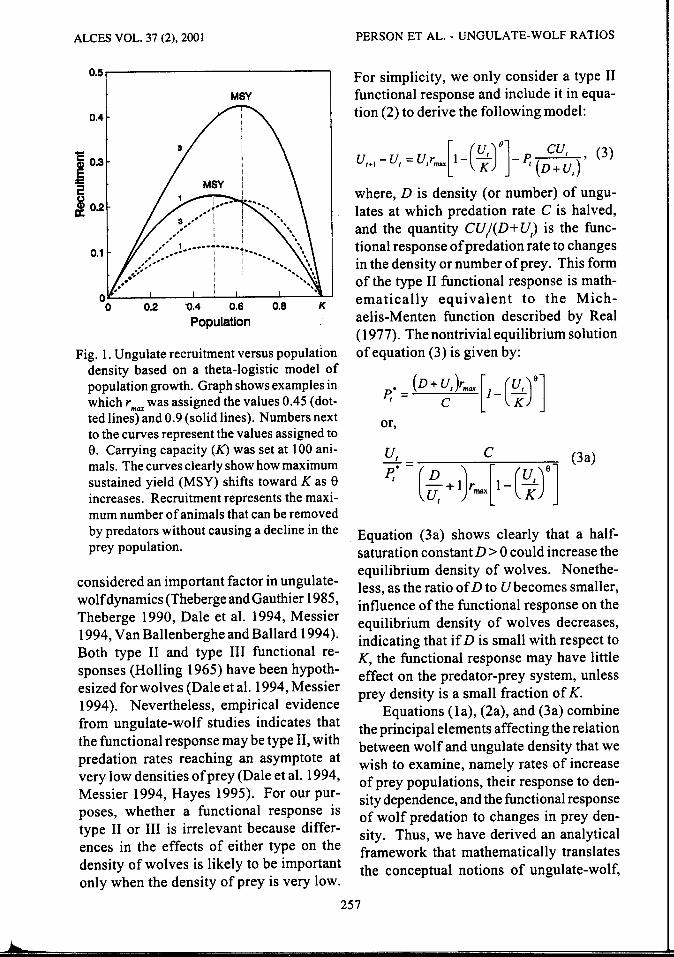
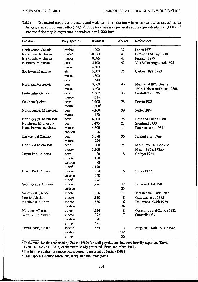
Number of predators supported by prey increases as the density of the prey popula­tion approaches maximum sustained yield (MSY), and declines after density exceeds MSY and approaches K (Fig. 1; Fowler 1987; McCullough 1987, 1999). Further, if 2 prey species have similar values of r max'

but one species exhibits density-dependent recruitment indicative of a higher value ofS, MSY will be shifted closer to K; this param­eter is given by the second derivative of the theta-logistic function:

[~]i 8+1

The species with the higher value of S will support a greater density of predators at equilibrium (Fig. 1 ).

The functional response in rates of pre­dation by wolves on ungulate prey has been

256

ALCES VOL. 37 (2), 2001

0.5..----------------,

0.4

'E J 0.3

2 ~ 0.2

0.1

...

MSY

)······.,.. .. .. ··:: .. !-·····r··-- ·----....

,' ,.•' .-::-" ..

0.2 '0.4 0.6 0.8

Population

Fig. 1. Ungulate recruitment versus population density based on a theta-logistic model of population growth. Graph shows examples in which rmax was assigned the values 0.45 (dot­ted lines) and 0.9 (solid lines). Numbers next to the curves represent the values assigned to e. Carrying capacity (K) was set at 100 ani­mals. The curves clearly show how maximum sustained yield (MSY) shifts toward K as 8 increases. Recruitment represents the maxi­mum number of animals that can be removed by predators without causing a decline in the prey population.

considered an important factor in ungulate­wolf dynamics (Theberge and Gauthier 1985, Theberge 1990, Dale et al. 1994, Messier 1994, Van Ballenberghe and Ballard 1994 ). Both type II and type III functional re­sponses (Holling 1965) have been hypoth­esized for wolves (Dale et al. 1994, Messier 1994). Nevertheless, empirical evidence from ungulate-wolf studies indicates that the functional response may be type II, with predation rates reaching an asymptote at very low densities of prey (Dale et al. 1994, Messier 1994, Hayes 1995). For our pur­poses, whether a functional response is type II or III is irrelevant because differ­ences in the effects of either type on the density of wolves is likely to be important only when the density of prey is very low.

PERSON ET AL.- UNGULATE-WOLF RATIOS

For simplicity, we only consider a type II functional response and include it in equa­tion (2) to derive the following model:

_ [ (u')o] cu, (3) Ut+l - U, - U,r max l - K - P, ( D + U,) '

where, D is density (or number) of ungu­lates at which predation rate C is halved, and the quantity CU/(D+ U,) is the func­tional response of predation rate to changes in the density or number of prey. This form of the type II functional response is math­ematically equivalent to the Mich­aelis-Menten function described by Real ( 1977). The nontrivial equilibrium solution of equation (3) is given by:

P,. = (n+~,)rmax [1-(ir] or,

u, c

P,' ~ (~ +1}~[~-(i)'] (3a)

Equation (3a) shows clearly that a half­saturation constant D > 0 could increase the equilibrium density of wolves. Nonethe­less, as the ratio of D to Ubecomes smaller, influence of the functional response on the equilibrium density of wolves decreases, indicating that if D is small with respect to K, the functional response may have little effect on the predator-prey system, unless prey density is a small fraction of K.

Equations (la), (2a), and (3a) combine the principal elements affecting the relation between wolf and ungulate density that we wish to examine, namely rates of increase of prey populations, their response to den­sity dependence, and the functional response of wolf predation to changes in prey den­sity. Thus, we have derived an analytical framework that mathematically translates the conceptual notions of ungulate-wolf,

257

UNGULATE-WOLF RATIOS- PERSON ET AL.

predator-prey dynamics (which likely are relevant for most predator-prey systems involving large terrestrial mammals), ena­bling us to address the following questions: I. With respect to predictions made by

equation (I a), data from studies in which biomass available to wolves is estimated for individual species of prey and com­pared with estimates of wolf density, should show species-specific differences in the density of wolves supported by a given unit of biomass. Those trends should be consistent with our hypothesis that ungulate species with higher rates of population increase such as deer would support more wolves per unit ofbiomass than populations with lower rates of in­crease such as moose and caribou (Rangifer tarandus).

2. How sensitive is the number ofwolves at equilibrium to effects of density depend­ence on growth rates of prey populations and their proximity to K? Would this sensitivity seriously confound the inter­pretation ofungulate-wolfratios or other indices of ungulate density (or biomass) versus wolf density used to assess ef­fects of predation on prey populations?

3. How sensitive is the number of wolves supported at equilibrium to the functional response, and would this sensitivity con­fuse interpretation of ungulate-wolf ra­tios or other indices of ungulate density (or biomass) versus wolf density?

A Stochastic Model of Ungulate-wolf Equilibrium

Superficial interpretation of relative wolf and ungulate densities to determine popula­tion trajectories of wolves and their prey potentially is misleading unless factors that we have discussed previously are consid­ered. Herein we describe a stochastic model that predicts the number of wolves that could be supported by a particular density of prey without causing a decline in

ALCES VOL. 37 (2), 2001

prey numbers. As shown in equation (Ia), theoretical

equilibrium is reached when wolf predation removes a number of ungulates equal to the annual recruitment (Ux r), provided preda­tion is primarily a source of additive mortal­ity (Mech and Karns 1977, Keith 1983, Hayes 1995). Ungulates are pulse breed­ers, so population growth may be expressed in the discrete form:

Ur+I = U, +U,r• where, t represents 1 year and U, is the preparturient ungulate population in the ab­sence of predation. The finite rate of in­crease, 'A, is given by:

Described in this manner, A encom­passes reproduction, emigration, immigra­tion, and all forms of compensatory mortal­ity. Substituting A for r in equation (1a) yields:

• U, ( ) or U, C (4) P, = C 'A -1 P,. = (A. -1) .

The theoretical number of ungulates per wolf required for equilibrium in our model can be computed by equation (4). If other additive sources of mortality exist, such as other predators or human hunters, the fraction of the ungulate population that can be removed by wolves that will result in a stationary ungulate population is reduced, and the model can be modified in the follow­ing way:

P,• = ~('A -1){1- H)

or,

u, c P,• = ('A- 1)( 1- H),

(5)

258

ALCES VOL. 37 (2), 2001

where, H is the fraction of annual recruit­ment removed by other predators or hunting by humans. This is the model, or equilibrium function, proposed by Keith (1983) to esti­mate ungulate-wolf ratios necessary to maintain a stationary population of prey.

Behavior of the equilibrium function (Keith 1983) can be understood by letting UjP* =Nand taking first-order partial de­rivatives with respect to input variables:

8N 1 BC = (A.-1)(1-H), for A. > 1 and H < 1 (Sa)

aN - C forA.> 1 andH< 1(5b) - ' a1.. - (A. -1) 2(1- H)

aN C for A. > 1 andH < 1(5c) aH = (A. -1)(1- H) 2

'

Predation rate C is a constant; there­fore, change in N for a particular predation rate is solely a function of A. and H (equation [5a]). Although predation rates may vary with changes in prey density, we will show in our analysis of equation (3a) that under most circumstances, the functional response of predation by wolves can be ignored. Equations ( 5b) and ( 5c) indicate that changes inN with respect to A. or Hare nonlinear, dependent on the instantaneous values of A. and H, and likely dominate behavior of the model. Clearly, as A. and H ~ 1, N ~oo in a rapidly increasing fashion.

Predicted ratios of ungulates to wolves at equilibrium (N) that are lower than ratios observed in the wild imply that prey populations will increase regardless of pre­dation by wolves. In contrast, if predicted ratios at equilibrium are greater than ob­served ratios of ungulates to wolves, prey populations likely will decline as a result of predation. Ungulate-wolf ratios observed in the wild that are equal to equilibrium ratios predicted by the model would indicate

PERSON ET AL.- UNGULATE-WOLF RATIOS

potential for stability in the predator-prey system. Nevertheless, time lags in the numerical response of wolves to changes in prey density and stochastic events such as severe winters must be considered before stability can be assumed.

Our model is useful for understanding multiple-prey systems because prey selec­tion by wolves would be reflected in the predation rate observed for each species involved. This procedure is an advantage over simple comparisons of total biomass of prey to wolf density, which do not compen­sate for prey selectivity by wolves. Our model, however, does not deal with numeri­cal responses of wolves to changing density of prey. For instance, Seip (1992) hypoth­esized that wolves did not decline with a decreasing population of caribou because a larger population of moose sustained those canids. That outcome may reflect wolves sometimes selecting caribou as prey in pref­erence to moose (Dale et al. 1994). Barten et al. (200 1) reported substantial effects of large mammalian carnivores on the ecology and behavior of a small population of cari­bou in a system where moose density also was low. Further, Gasaway et al. (1992) noted that moose were held at low density while caribou populations varied. The for­going examples, however, are unlikely to alter the general conclusions of our model­those results are for extremely low-density populations of ungulates where prey switch­ing by wolves, and potential changes in the type of their functional response, are rela­tively unimportant.

Unfortunately, the equilibrium function is deterministic, and input variables are as­sumed to be measured without error. This assumption poses no real problem when the function is used as a theoretical device, but is a serious limitation if the equation is applied empirically. Estimates of A. and H must be precise; error in estimation of A., particularly when the ungulate population

259

UNGULATE-WOLF RATIOS- PERSON ET AL.

nears K, may result in equilibrium ratios very different from ratios that would be predicted if the true value of A. were known. Effects on sensitivity of the model to values of A. and H near 1, combined with sampling errors associated with input variables, may result in predicted ratios of equilibrium that are possibly misleading or even meaning­less.

The equilibrium function would be more useful for interpreting data from the field if outcomes were probabilistic, reflecting er­ror in the variable inputs and accommodat­ing the potential sensitivity of the model to levels of input variables. That result can be achieved by incorporating input variables that are random samples rather than dis­crete values. In most instances where predation rate (C), A., and mortality caused by other predators (H) are estimated em­pirically, those estimates will be sample means and their standard deviations. As­suming the sample was extracted from a population exhibiting a specific statistical distribution, a random sample from the prob­ability density functions (pdf) of each vari­able can be substituted for the discrete values used as input in the equilibrium func­tion. The model retains the same general form as equation (5):

C' N' = (a,b) ' (6) (A' (a,b) -1}(1- H'(a,b)}

where, N' = [N,, N2, Nr··Nn], vector of solu­tiotn'~ for equilibrium ratios, C' = [CI' C2, C3, ••• , Cn], a random sam­pl~·~rom the pdfofCwithparameters a and b representing upper and lower limits of a range as in a uniform distribution, or a mean and SD as in a normal distribution, A.' = [A.I' A.2, A.3, ... , A.n], a random sample fr8'J{ the pdf of A. with parameters a and b as defined for C', and

H' = [H1, H2, H3, ... , Hn], a random sam­(a,bJ

ALCES VOL. 37 (2), 2001

pie from the pdf of H with parameters a and b as defined for C'.

Equation (6) is a natural extension of the original model described by Keith ( 1983 ), and is appropriate for any potential sam­pling distribution. Assuming that each pa­rameter is an independent random variable, the variance of N' can be approximated by:

[BNJ2

[BNJ2

[BNJ2

Var(N~ = Var(C') BC + Var(A.') Bl.. + Var(H~ BH

(Seber 1982). Substituting equations ( 5a-c) into the equation for Var(N') yields:

Var{N') = Var(C'{(A. -I): I- H) J + Var(A.'{(A. _ 1)z~ _H) r + Var(H~[ (A._!)~_ H) 2 r. (?)

We conduct a series of simulations of equation (6) to describe the behavior of the model and to illustrate its limitations and application to data from the field.

METHODS We analyzed data relating ungulate

biomass to density ofwolves (Fuller 1989) to test for species-specific differences in number of wolves supported by a particular biomass of ungulate prey. Following the method of Fuller ( 1989), prey biomass was converted to equivalent units such that one unit of biomass equaled 1 deer (Table 1 ). Biomass units representing individual spe­cies were as follows: 1 bison (Bison bison) = 8 units, 1 moose = 6 units, 1 elk ( Cervus elaphus) = 3 units, 1 caribou= 2 units, and 1 mountain sheep (Ovis sp.), 1 mountain goat (Oreamnos americanus), or 1 deer (Odocoileus sp.) = 1 unit. We regressed biomass units by species against wolf den­sity and used F tests of the differences between the error sum of squares for full and reduced models to test for differences between regression coefficients (Neter et al. 1985).

260

ALCES VOL. 37 (2), 2001 PERSON ET AL.- UNGULATE-WOLF RATIOS

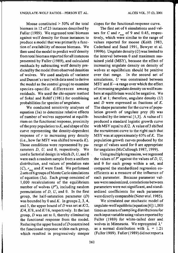
Table I. Estimated ungulate biomass and wolf densities during winter in various areas of North America, adapted from Fuller ( 1989)1• Prey biomass is expressed as deer equivalents per 1,000 km2

and wolf density is expressed as wolves per 1,000 km2•

Location Prey species Biomass Wolves References

North-central Canada caribou 11,000 37 Parkerl973 Isle Royale, Michigan moose 10,570 40 Peterson and Page 1988 Isle Royale, Michigan moose 9,696 43 Peterson 1977 Northeast Minnesota deer 5,100 42 VanBallenbergheetal.l975

moose 4,200 Southwest Manitoba elk 3,600 26 Carbyn 1982, 1983

moose 4,800 deer 340

Northeast Minnesota deer 3,500 40 Mech eta! 1971, Peek et al. moose 3,600 1976, Nelson and Mech l986b

East-central Ontario deer 5,769 38 Pimlott et al. 1969 moose 1,014

Southern Quebec deer 3,000 28 Potvin 1988 moose 3,6002

North-central Minnesota deer 6,160 39 Fuller 1989 moose 120

North-central Minnesota deer 6,000 28 Berg and Kuehn 1980 Northeast Minnesota deer 3,475 23 Stenlund 1955 Kenai Peninsula, Alaska moose 4,800 14 Peterson et al. 1984

caribou 26 East-central Ontario deer 3,098 36 Pimlott et al. 1969

moose 924 Northeast Minnesota deer 600 25 Mech 1986, Nelson and

moose 3,300 Mech l986a, 1986b Jasper Park, Alberta deer 80 8 Carbyn 1974

moose 480 caribou 80 other-3 2,170

Denali Park, Alaska moose 984 6 Haberl977 caribou 540 other-3 478

South-central Ontario moose 1,776 12 Bergerud et al. 1983 caribou 26

Southwest Quebec moose 1,800 11 Messier and Crete 1985 Interior Alaska moose 1,110 8 Gasaway et al. 1983 Northeast Alberta moose 1,350 6 Fuller and Keith 1980

caribou 34 N orthem Alberta other-3 1,224 8 Oosenbrug and Carbyn 1982 West-central Yukon moose 372 7 Sumanik 1987

caribou 20 other-3 681

Denali Park, Alaska moose 564 3 SingerandDalle-Molle 1985 caribou 212 other-3 86

1 Table excludes data reported by Fuller ( 1989) for wolf populations that were heavily exploited (Davis 1978, Ballard et al. 1987) or that were newly protected (Fritts and Mech 1981 ).

2 The biomass value for moose was incorrectly reported by Fuller ( 1989). 3 Other species include bison, elk, sheep, and mountain goats.

261

UNGULATE-WOLF RATIOS - PERSON ET AL.

Moose constituted > 50% of the total biomass in 12 of 23 instances described by Fuller ( 1989). We regressed total biomass against wolf density for those instances to produce a model that was primarily a func­tion of availability of moose biomass. We then used the model to predict wolf density from total biomass reported for all instances presented by Fuller ( 1989), and calculated residuals by subtracting wolf density pre­dicted by the model from observed densities of wolves. We used analysis of variance and Dunnet's t test (with data used to derive the model as the control group) to examine species-specific differences among residuals. We used the chi-square method of Sokal and Rohlf ( 1981) for combining probabilities for species of ungulates.

We conducted sensitivity analyses of equation (3a) to determine relative effects of number of wolves supported at equilib­rium on the functional response, proximity of the prey population to K, and shape of the curve representing the density-dependent response of r to increasing prey density (i.e., how far MSY was shifted towards K). Those conditions were represented by pa­rameters D, U, and e, respectively. We used a factorial design in which D, U, and e were each a random sample from a uniform distribution, and values of predation rate (C), r max and K were fixed. We performed 2 sets of6 groups ofMonte Carlo simulations of equation (3a). Each group consisted of 1,000 recalculations of the equilibrium number of wolves (F*), including random permutations of D, U, and e. In the first group, the half-saturation parameter (D) was bounded by 0 and K. In groups 2, 3, 4, and 5, the upper bound of D was set at K/2, K/4, K/8, and K/16, respectively. In the last group, D was set to 0, thereby eliminating the functional response from the model. Reducing the upper bound of D constrained the functional response within each group, which resulted in progressively steeper

ALCES VOL. 37 (2), 2001

slopes for the functional-response curve. The first set of 6 simulations used val­

ues for C and r of 9 and 0.45, respec-max

tively, which were similar to the range of values reported for moose (Keith 1983, Cederlund and Sand 1991, Bowyer et al. 1999b ). Ungulate density ( U) was limited to the interval between 0 and maximum sus­tained yield (MSY), because the effect of increasing ungulate density on density of wolves at equilibrium should be positive over that range. In the second set of simulations, U was constrained between MSY and K -a range over which the effect of increasing ungulate density on wolf num­bers at equilibrium would be negative. We set K at 1; therefore, ungulate density ( U) and D were expressed as fractions of K. The shape parameter for the curve of popu­lation growth of ungulate prey (8) was bounded by the interval [1,3]. A value of 1 produced a standard logistic growth curve with MSY equal to K/2. A value of3 shifted the recruitment curve to the right such that MSY was at approximately 63% of K. The population growth curves produced by the range of values used for e are appropriate for ungulates (McCullough 1987, 1999).

Using multiple regression, we regressed the values of p* against the values of D, U, and e for each group within a set, and

.·compared the standardized regression co­efficients as a measure of the influence of each parameter. Because parameter val­ues were randomized, correlations between parameters were not significant, and stand­ardized coefficients for each parameter were directly comparable (Neteret al. 1985).

We simulated our stochastic model of ungulate-wolf equilibria (equation [ 6]) 1,000 times as means of sampling distributions for each input variable using values reported by Fuller ( 1989) for white-tailed deer and wolves in Minnesota. We repre~nted A' as a normal distribution with A = 1.21 (Fuller 1989). Fuller ( 1989) did not report a

262

ALCES VOL. 37 (2), 2001

variance about that value of A.; therefore, we arbitrarily assigned a SD = 0.03. Con­sequently, 95% of the values in a random sample from the distribution of A' were between 1.15 and 1.27 (± 5% of the mean, or 2 SD). In addition, we represented C' as a normal distribution with C = 19 and SD = 0.5, resulting in 95% of the values in a random sample from C' occurring within 5% of the mean. Similar to Fuller ( 1989), we let H = 0. Without changing the distri­butions of C' and H', we repeated simulations of the model with A' repre­sented by a normal distribution with I = 1.1 and SD = 0.03. We generated a sampling distribution for each variable in the model by multiplying random normal deviates by the SD of each input variable.

RESULTS Factors Affecting the Relation Between Wolf and Ungulate Density

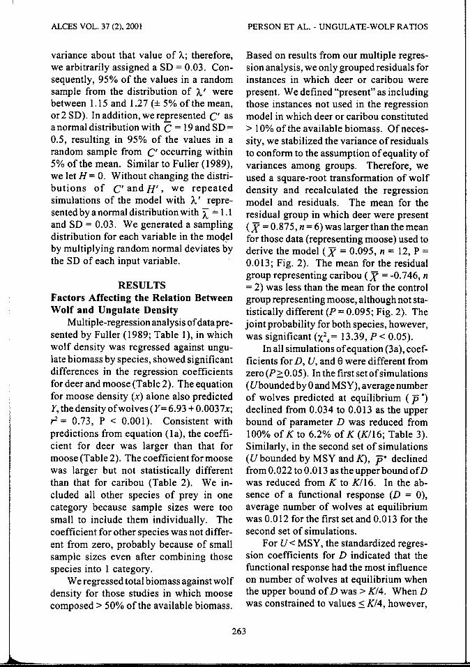
Multiple-regression analysis of data pre­sented by Fuller (1989; Table 1 ), in which wolf density was regressed against ungu­late biomass by species, showed significant differences in the regression coefficients for deer and moose (Table 2). The equation for moose density (x) alone also predicted Y, thedensityofwolves (Y= 6.93 +0.0037x; r = 0.73, P < 0.001). Consistent with predictions from equation ( 1 a), the coeffi­cient for deer was larger than that for moose (Table 2). The coefficient for moose was larger but not statistically different than that for caribou (Table 2). We in­cluded all other species of prey in one category because sample sizes were too small to include them individually. The coefficient for other species was not differ­ent from zero, probably because of small sample sizes even after combining those species into 1 category.

We regressed total biomass against wolf density for those studies in which moose composed> 50% of the available biomass.

PERSON ET AL.- UNGULATE-WOLF RATIOS

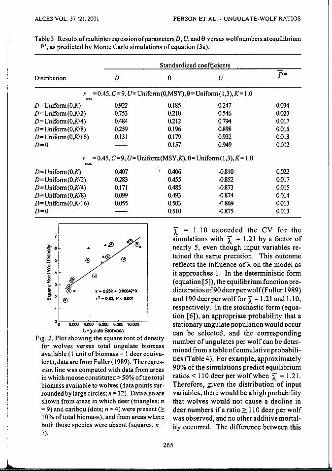
Based on results from our multiple regres­sion analysis, we only grouped residuals for instances in which deer or caribou were present. We defined "present" as including those instances not used in the regression model in which deer or caribou constituted > 1 0% of the available biomass. Of neces­sity, we stabilized the variance of residuals to conform to the assumption of equality of variances among groups. Therefore, we used a square-root transformation of wolf density and recalculated the regression model and residuals. The mean for the residual group in which deer were present (X= 0.875, n = 6) was larger than the mean for those data (representing moose) used to derive the model (X = 0.095, n = 12, P = 0.013; Fig. 2). The mean for the residual group representing caribou (X= -0.746, n = 2) was less than the mean for the control group representing moose, although not sta­tistically different (P = 0.095; Fig. 2). The joint probability for both species, however, was significant (X2

4 = 13.39, P < 0.05).

In all simulations of equation (3a), coef­ficients forD, U, and e were different from zero (P 2:. 0.05). In the first set of simulations ( Ubounded by 0 and MSY), average number of wolves predicted at equilibrium ( p •) declined from 0.034 to 0.013 as the upper bound of parameter D was reduced from 100% of K to 6.2% of K (K/16; Table 3). Similarly, in the second set of simulations ( U bounded by MSY and K), p• declined from 0.022 to 0.013 as the upper bound of D was reduced from K to K/16. In the ab­sence of a functional response (D = 0), average number of wolves at equilibrium was 0.012 for the first set and 0.013 for the second set of simulations.

For U < MSY, the standardized regres­sion coefficients for D indicated that the functional response had the most influence on number of wolves at equilibrium when the upper bound of D was > K/4. When D was constrained to values :S K/4, however,

263

UNGULATE-WOLF RATIOS- PERSON ET AL. ALCES VOL. 37 (2), 2001

Table 2. Results from multiple regression of ungulate biomass 1 versus wolf density with tests of coefficients. Data are from Fuller ( 1989)2•

Species Coefficient(~) SE p

Constant 3.93 2.07 1.90 0.074 Deer 0.0051 0.001 9.71 0.000 Moose 0.0036 0.000 8.74 0.000 Caribou 0.0030 0.001 5.81 0.000 Otheil 0.0010 0.001 0.76 0.459

Model: #Wolves/1000km2 =3.93+0.0051(Biomass )+0.0036(Biomass )+

deer moose

0.003(Biomass )+0.001(Biomass }+E caribou other

F= 37.4, P<0.0001, AdjustedR2 = 0.87, n = 23

Tests of Coefficients:

H: ~ =~ H:~ =~ 0 deer moose 0 moose caribou

H: ~ *~ H:~ *~ a deer moose a moose caribou

F =7.10, P=0.02 F = 1.01, P=0.35 1,18 1,18

1 Ungulate biomass is represented as deer equivalents per 1,000 km2 such that 1 moose= 6 deer, 1 elk = 3 deer, 1 caribou= 2 deer, 1 bison= 8 deer, and 1 sheep or goat= 1 deer (Fuller 1989).

2 Data presented in Fuller ( 1989) for a heavily exploited wolf population (Davis 1978, Ballard et al. 1987) and for a newly protected wolf population (Fritts and Mech 1981) were excluded.

3 Includes bison, mountain sheep, and mountain goats.

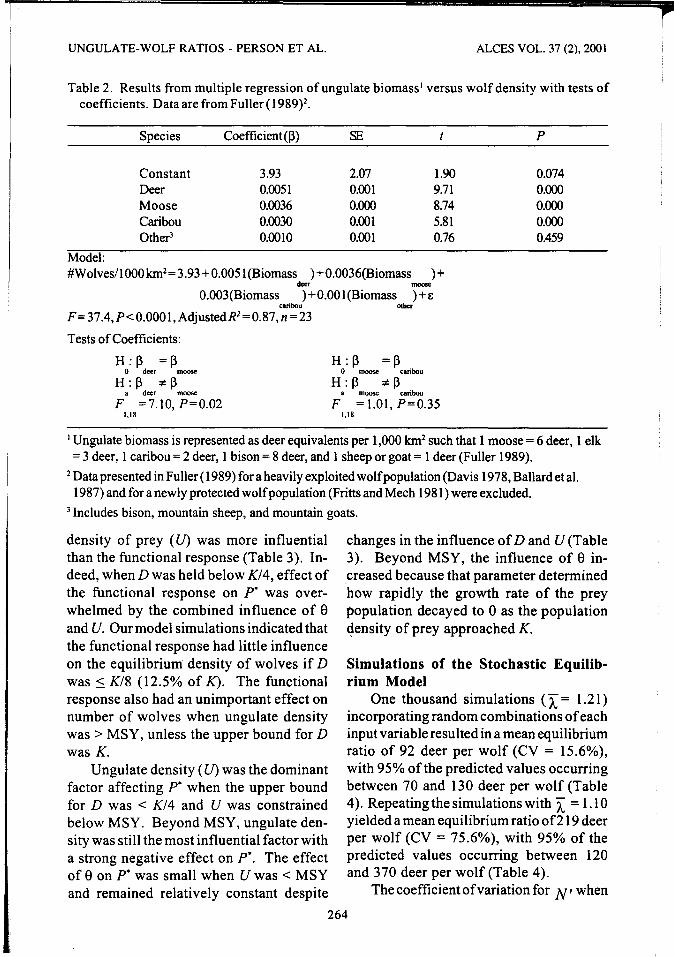
density of prey ( U) was more influential than the functional response {Table 3). In­deed, when D was held below K/4, effect of the functional response on p* was over­whelmed by the combined influence of e and U. Our model simulations indicated that the functional response had little influence on the equilibrium density of wolves if D was :5 K/8 (12.5% of K). The functional response also had an unimportant effect on number of wolves when ungulate density was> MSY, unless the upper bound forD was K.

Ungulate density ( U) was the dominant factor affecting p* when the upper bound forD was < K/4 and U was constrained below MSY. Beyond MSY, ungulate den­sity was still the most influential factor with a strong negative effect on?*. The effect of e on p* was small when U was < MSY

changes in the influence of D and U (Table 3). Beyond MSY, the influence of 8 in­creased because that parameter determined how rapidly the growth rate of the prey population decayed to 0 as the population density of prey approached K.

Simulations of the Stochastic Equilib­rium Model

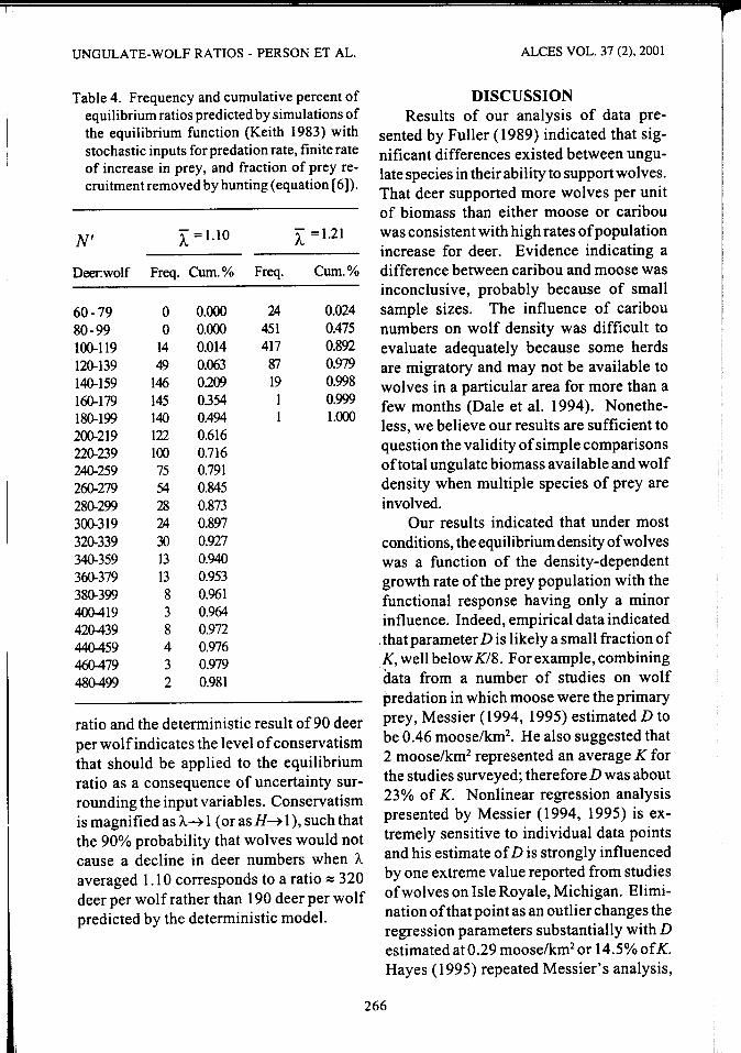
One thousand simulations (I"= 1.21) incorporating random combinations of each input variable resulted in a mean equilibrium ratio of 92 deer per wolf (CV = 15.6%), with 95% of the predicted values occurring between 70 and 130 deer per wolf (Table 4 ). Repeating the simulations with ~ = 1.10 yielded a mean equilibrium ratio of219 deer per wolf (CV = 75.6%), with 95% of the predicted values occurring between 120 and 370 deer per wolf (Table 4).

and remained relatively constant despite 264

The coefficient of variation for N' when

....

ALCES VOL. 37 (2), 2001 PERSON ET AL.- UNGULATE-WOLF RATIOS

Table 3. Results of multiple regression of parameters D, U, and 8 versus wolf numbers at equilibrium P-, as predicted by Monte Carlo simulations of equation (3a).

Standardized coefficients

Distribution D e u P*

r =0.45,C=9, U=Uniform(O,MSY),9=Uniform(l,3),K= 1.0 max

D=Uniform(O.K) 0.922 0.185 0247 0.034 D=Uniform(O,K/2) 0.753 0210 0.546 0.023 D=Uniform(O,K/4) 0.484 0212 0.794 0.017 D= Uniform(O,K/8) 0259 0.196 0.898 O.ol5 D=Uniform(O,K/16) 0.131 0.179 0.932 0.013 D=O - 0.157 0.949 0.012

r =0.45, C=9, U=Unifornt(MSY .K),9=Uniform(1,3),K= 1.0 max

D=Uniform(O.K) 0.407 D= Uniform(O,K/2) 0283 D=Uniform(O,K/4) 0.171 D= Uniform(O,K/8) 0.099 D= Uniform(O,K/16) 0.055 D=O -

7

f ·[ • •llJ ;?®. c! 5 ® .!P' @ = ~ 4

~ r @ /@ ~ 3 ~ Y • 2.282 + 0.(1()()42-X

/jf 2 (!) r 2 • 0.82, P < 0.001

0 0 2,000 4,000 6,000 8,000 10,000

Ungulate Biomass

Fig. 2. Plot showing the square root of density for wolves versus total ungulate biomass available (l unit of biomass= 1 deer equiva­lent); data are from Fuller ( 1989). The regres­sion line was computed with data from areas in which moose constituted> 50% of the total biomass available to wolves (data points sur­rounded by large circles; n = 12). Data also are shown from areas in which deer (triangles; n = 9) and caribou (dots; n = 4) were present (2: 10% oftotal biomass), and from areas where both those species were absent (squares; n = 7).

0.406 -0.810 0.022 0.455 -0.852 0.017 0.485 -0.873 0,015 0.493 -0.874 0.014 0.503 -0.869 0.013 0.510 -0.875 0.013

I = 1.10 exceeded the CV for the simulations with I = 1.21 by a factor of nearly 5, even though input variables re­tained the same precision. This outcome reflects the influence of A. on the model as it approaches 1. In the deterministic form (equation [ 5]), the equilibrium function pre­dicts ratios of90 deerperwolf(Fuller 1989) and 190 deerperwolffor I= 1.21 and 1.1 0, respectively. In the stochastic form (equa­tion [6]), an appropriate probability that a stationary ungulate population would occur can be selected, and the corresponding number of ungulates per wolf can be deter­mined from a table of cumulative probabili­ties {Table 4 ). For example, approximately 90% of the simulations predict equilibrium ratios < 110 deer per wolf when I = 1.21. Therefore, given the distribution of input variables, there would be a high probability that wolves would not cause a decline in deer numbers if a ratio 2: 110 deer per wolf was observed, and no other additive mortal­ity occurred. The difference between this

265

UNGULATE-WOLF RATIOS- PERSON ET AL.

Table 4. Frequency and cumulative percent of equilibrium ratios predicted by simulations of the equilibrium function (Keith 1983) with stochastic inputs for predation rate, finite rate of increase in prey, and fraction of prey re-cruitment removed by hunting (equation [ 6]).

N' ~ = 1.10 ~ =1.21

Deer:wolf Freq. Cum.% Freq. Cum.%

60-79 0 0.000 24 0.024 80-99 0 0.000 451 0.475 100-119 14 0.014 417 0.892 120-139 49 0.063 87 0.979 140-159 146 0209 19 0.998 160-179 145 0.354 I 0.999 180-199 140 0.494 I 1.000 200-219 122 0.616 220-239 100 0.716 240-259 75 0.791 260-279 54 0.845 280-299 28 0.873 300-319 24 0.897 320-339 30 0.927 340-359 13 0.940 360-379 13 0.953 380-399 8 0.961 400-419 3 0.964 420-439 8 0.972 440-459 4 0.976 460-479 3 0.979 480-499 2 0.981

ratio and the deterministic result of90 deer per wolf indicates the level of conservatism that should be applied to the equilibrium ratio as a consequence of uncertainty sur­rounding the input variables. Conservatism is magnified as A.~ 1 (or asH~ 1 ), such that the 90% probability that wolves would not cause a decline in deer numbers when A. averaged 1.1 0 corresponds to a ratio ~ 320 deer per wolf rather than 190 deer per wolf predicted by the deterministic model.

ALCES VOL. 37 (2), 2001

DISCUSSION Results of our analysis of data pre­

sented by Fuller (1989) indicated that sig­nificant differences existed between ungu­late species in their ability to support wolves. That deer supported more wolves per unit of biomass than either moose or caribou was consistent with high rates of population increase for deer. Evidence indicating a difference between caribou and moose was inconclusive, probably because of small sample sizes. The influence of caribou numbers on wolf density was difficult to evaluate adequately because some herds are migratory and may not be available to wolves in a particular area for more than a few months (Dale et al. 1994). Nonethe­less, we believe our results are sufficient to question the validity of simple comparisons oftotal ungulate biomass available and wolf density when multiple species of prey are involved.

Our results indicated that under most conditions, the equilibrium density of wolves was a function of the density-dependent growth rate of the prey population with the functional response having only a minor influence. Indeed, empirical data indicated . that parameter Dis likely a small fraction of K, well below K/8. For example, combining data from a number of studies on wolf predation in which moose were the primary prey, Messier (1994, 1995) estimated D to be 0.46 moose/km2• He also suggested that 2 moose/km2 represented an average K for the studies surveyed; therefore D was about 23% of K. Nonlinear regression analysis presented by Messier (1994, 1995) is ex­tremely sensitive to individual data points and his estimate of Dis strongly influenced by one extreme value reported from studies of wolves on Isle Royale, Michigan. Elimi­nation of that point as an outlier changes the regression parameters substantially with D estimated at 0.29 moose/km2 or 14.5% of K. Hayes (1995) repeated Messier's analysis,

266

' II,

ALCES VOL. 37 (2), 2001

but included data from his own study on rates of predation on moose in the Yukon, Canada, and estimatedD at only 0.07 moose/ km2 or 3.5% of K. Dale et al. (1994) described a functional response for wolves preying on caribou that indicated a half­saturation constant equal to about 0.026 caribou/km2 or about 1.1% of the maximum density of caribou observed in their study. Viewed in conjunction with our model simulations, those data indicate that the functional response may be relatively unim­portant to the dynamics between wolves and their ungulate prey except when prey populations are at low densities.

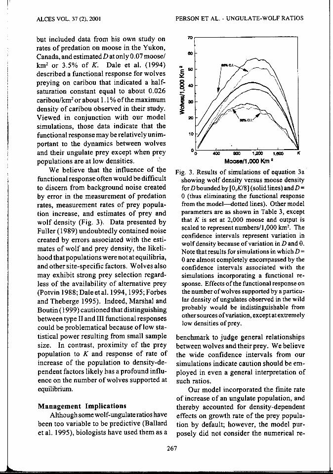
We believe that the influence of the functional response often would be difficult to discern from background noise created by error in the measurement of predation rates, measurement rates of prey popula­tion increase, and estimates of prey and wolf density (Fig. 3). Data presented by Fuller ( 1989) undoubtedly contained noise created by errors associated with the esti­mates of wolf and prey density, the likeli­hood that populations were not at equilibria, and other site-specific factors. Wolves also may exhibit strong prey selection regard­less of the availability of alternative prey (Potvin 1988; Dale et al. 1994, 1995; Forbes and Theberge 1995). Indeed, Marshal and Boutin ( 1999) cautioned that distinguishing between type II and III functional responses could be problematical because oflow sta­tistical power resulting from small sample size. In contrast, proximity of the prey population to K and response of rate of increase of the population to density-de­pendent factors likely has a profound influ­ence on the number of wolves supported at equilibrium.

Management Implications Although some wolf-ungulate ratios have

been too variable to be predictive (Ballard et al. 1995), biologists have used them as a

PERSON ET AL.- UNGULATE-WOLF RATIOS

~~---------------------------.

eo

N

~60

~40 }ao ~

20

10

400 800 1 ,200 1,800

Moose/1 ,000 Km 2

Fig. 3. Results of simulations of equation 3a showing wolf density versus moose density for Dbounded by [O,K/8] (solid lines) andD= 0 (thus eliminating the functional response from the model-dotted lines). Other model parameters are as shown in Table 3, except that K is set at 2,000 moose and output is scaled to represent numbers/1,000 km2

• The confidence intervals represent variation in wolf density because of variation in D and e. Note that results for simulations in which D = 0 are almost completely encompassed by the confidence intervals associated with the simulations incorporating a functional re­sponse. Effects of the functional response on the number of wolves supported by a particu­lar density of ungulates observed in the wild probably would be indistinguishable from other sources of variation, except at extremely low densities of prey.

benchmark to judge general relationships between wolves and their prey. We believe the wide confidence intervals from our simulations indicate caution should be em­ployed in even a general interpretation of such ratios.

Our model incorporated the finite rate of increase of an ungulate population, and thereby accounted for density-dependent effects on growth rate of the prey popula­tion by default; however, the model pur­posely did not consider the numerical re-

267

UNGULATE-WOLF RATIOS- PERSON ET AL.

sponse of wolves to their ungulate prey. Likewise, densities of ungulates and wolves measured in the field often are point esti­mates in time, and the population trajectory of wolves before or after the measurement period usually is not considered when deter­mining whether predation may cause a de­cline in ungulate numbers. Clearly, the numerical response of wolves is important to the stability of the predator-prey system, and likely would produce additional variabil­ity in predator-prey ratios. This likely out­come requires further conservatism in ap­plying wolf-ungulate ratios to manage large carnivores and their ungulate prey.

We also caution that equilibrium ratios will increase rapidly as the prey population exceeds the point at which MSY is achieved. Consequently, confidence intervals sur­rounding predicted equilibrium ratios would become very large even if').., was estimated with high precision. Mortality from preda­tion likely would become increasingly com­pensatory as prey populations exceeded MSY and approachedK (McCullough 1979); thus, the assumption that mortality from predation was additive would be violated. At what point the transition of predation from additive to compensatory mortality would seriously affect the interpretation of ungulate-wolf ratios is unknown and war­rants further study.

Some biologists may object to our reli­ance on the measure of K as a guide for interpreting effects of functional responses and density-dependent growth rates of prey populations on ungulate-wolf ratios. Carry­ing capacity often is viewed as a Chimera; an abstraction rather than a practical con­cept. Nevertheless, estimates of the poten­tial density of ungulates that an area can support have been used by biologists seek­ing to assess the effects of predation by wolves on ungulate populations (Gasaway et al. 1992). We suggest that these esti­mates be used as approximate measures of

ALCES VOL. 37 (2), 2001

K. We also advocate incorporating meas­ures of animal and range condition to help calibrate the position of the population with respect to K. Without some index to K, comparisons of rates of increase between populations are not valid (Bowyer et al. 1999b).

The functional response in rates of pre­dation by wolves to changes in ungulate density has been the focus of numerous studies (Theberge 1990, Dale et al. 1994, Messier 1994, Van Ballenberghe and Ballard 1994, Hayes 1995, Messier 1995, Seip 1995; Marshal and Boutin 1999). Our analyses indicate that rate of increase of ungulate populations is much more important than the functional response as a determinant of wolf density. We suggest that the limited resources available for conducting research on ungulate-wolf systems be concentrated on understanding the growth of prey populations with respect to habitat quality in relation to the predation behavior of wolves.

ACKNOWLEDGEMENTS Funding for this work was provided by

the Alaska Department of Fish and Game, the Alaska Cooperative Fish and Wildlife Research Unit, and the Institute of Arctic .J3iology at the University of Alaska Fairbanks. We are indebted to D. R. Klein for inspiring us to study wolf-ungulate dy­namics. We thank M. Castellini, D. R. Klein, A. D. McGuire, E. A. Rexstad, J. S. Sedinger, J. Schoen, and R. Sweitzer for helpful comments on this paper, and M. Kirchhoff for useful discussions of wolf­deer relations. We also thank M. Ingle for her editorial help.

REFERENCES ARDITI, R., and L. R. GINZBURG. 1989.

Coupling in predator-prey dynamics: ratio-dependence. Journal ofTheoreti­cal Biology 139:311-326.

BALLARD, w. B., L. A. AYRES, P. R.

268

ALCES VOL. 37 (2), 2001

KRAUSMAN, D.J. REED, andS. G. FANCY. 1997. Ecology ofwolves in relation to a migratory caribou herd in northwest Alaska. Wildlife Monographs 135.

___ , M. E. MCNAY, C. L. GARDNER, and D. J. REED. 1995. Use ofline-intercept track sampling for estimating wolf den­sities. Pages 469-480 in L. N. Carbyn, S. H. Fritts, and D. R. Seip, editors. Ecology and conservation of wolves in a changing world. Canadian Circumpolar Institute, Occasional Pub­lication Series, Number 35. Canadian Circumpolar Institute, Edmonton, Al-berta, Canada. '

___ , J. S. WHITMAN, and C. L. GARDNB~. 1987. Ecology of an exploited wolf population in south-central Alaska. Wildlife Monographs 98.

BARTEN, N. L., R .T. BowYER, and K. J. JENKINS. 200 1. Habitat use by female caribou: tradeoffs associated with par­turition. Journal of Wildlife Manage­ment 65:77-92.

BERG, W. E., and D. W. KuEHN. 1980. A study of the timber wolf population on the Chippewa National Forest. Minne­sota Natural Resources Quarterly 40:1-16.

BERGERUD, A. T., W. WYETT, and B. SNIDER. 1983. The role of wolf predation in limiting a moose population. Journal of Wildlife Management 4 7:977-988.

BERRYMAN, A. A. 1992. The origin and evolution of predator-prey theory. Ecol­ogy 73:1530-1535.

BLEICH, V. C., R. T. BowYER, and J. D. WEHAUSEN. 1997. Sexual segregation in mountain sheep: resources or preda­tion? Wildlife Monographs 134.

BoERTJE, R. D., and R. 0. StEPHENSON. 1992. Effects of ungulate availability on wolf reproductive potential in Alaska. Canadian Journal of Zoology 70:2441-2443.

BowYER, R. T. 1984. Sexual segregation in

PERSON ET AL.- UNGULATE-WOLF RATIOS

southern mule deer. Journal of Mammalogy 65:410-417.

---· 1987. Coyote group size relative to predation on mule deer. Mammalia 51:515-526.

___ , J. G. KIE, and V. VAN BALLENBERGHE. 1998a. Habitat selec­tion in neonatal black-tailed deer: cli­mate, forage, or risk of predation? Jour­nal ofMammalogy 79:415-425.

___ , M. c. NICHOLSON, E. M. MOLVAR, and J. B. FARO. 1999b. Moose on Kalgin Island: are density-dependent processes related to harvest? Alces 35:73-89.

___ , V. VAN BALLENBERGHE, and J. G. KIE. 1998b. Timing and synchrony of parturition in Alaskan moose: long-term versus proximal effects of climate. Journal ofMammalogy 79:1332-1344.

___ , and J. A. K. MAIER. 1999a. Birth-site selection by Alaskan moose: maternal strategies for coping with a risky environment. Jour­nal ofMammalogy 80:1070-1083.

CARBYN, L. N. 1974. Wolfpredation and behavioral interactions with elk and other ungulates in an area of high prey diver­sity. Canadian Wildlife Service Report, Edmonton, Alberta, Canada.

---· 1982. Incidence of disease and its potential role in the population dynam­ics of wolves in Riding Mountain Na­tional Park, Manitoba. Pages 106-116 in F. H. Harrington and P. C. Paquet, editors. Wolves of the world: perspec­tives on their behavior, ecology, and conservation. Noyes Publications, Park Ridge, New Jersey, USA.

---· 1983. Wolfpredation on elk in Riding Mountain National Park, Mani­toba. Journal ofWildlife Management 47:963-976.

CAUGHLEY,G. 1977. Analysisofvertebrate populations. John Wiley and Sons, New York, New York, USA.

269

UNGULATE-WOLF RATIOS- PERSON ET AL.

CEDERLUND, G. N., and H. K. G. SAND. 1991. Population dynamics and yield of a moose population without predators. Alces 27:31-40.

DALE, B. W., L. G. ADAMS, and R. T. BowYER. 1994. Functional response of wolves preying on barren-ground cari­bou in a multiple-prey ecosystem. Jour­nal of Animal Ecology 63:644-652.

______ ,and . 1995. Win-

ter wolf predation in a multiple ungulate prey system, Gates of the Arctic Na­tional Park, Alaska. Pages 223-230 in L. N. Carbyn, S. H. Fritts, and D. R. Seip, editors. Ecology and conservation of wolves in a changing world. Cana­dian Circumpolar Institute, Occasional Publication Series, Number 35. Cana­dian Circumpolar Institute, Edmonton, Alberta, Canada.

DAVIS, J. L. 1978. History and current status of Alaska caribou herds. Pages 1-8 in D. R. Klein and R. G. White, editors. Parameters of caribou popula­tion ecology in Alaska. Biological Pa­pers of the University of Alaska, Spe­cial Report, Number 4. University of Alaska, Fairbanks, Alaska, USA.

EBERHARDT, L. L. 1997. Is wolfpredation ratio-dependent? Canadian Journal of Zoology 75:1940-1944.

---· 1998. Applying difference equa­tions to wolf predation. Canadian Jour­nal of Zoology 76:380-386.

FoRBES, G. J., and J. B. THEBERGE. 1995. Influences of a migratory deer herd on wolf movements and mortality in and near Algonquin Park, Ontario. Pages 303-314 in L. N. Carbyn, S. H. Fritts, and D. R. Seip, editors. Ecology and conservation of wolves in a changing world. Canadian Circumpolar Institute, Occasional Publication Series, Number 35. Canadian Circumpolar Institute, Edmonton, Alberta, Canada.

FowLER, C. W. 1987. A review of density

ALCES VOL. 37 (2), 2001

dependence in populations oflarge mam­mals. Pages 410-441 in H. H. Genoways, editor. Current Mammalogy 1. Plenum Press, New York, New York, USA.

FRITTS, S. H., and L. D. MEcH. 1981. Dynamics, movements, and feeding ecology of a newly-protected wolf popu­lation in northwestern Minnesota. Wild­life Monographs 80.

FuLLER, T. K. 1989. Population dynamics of wolves in north-central Minnesota. Wildlife Monographs 105.

__ , and L. B. KEITH. 1980. Wolf population dynamics and prey relation­ships in northeastern Alberta. Journal ofWildlife Management 44:583-602.

GASAWAY, w. c., R. D. BOERTJE, D. v. GRANGAARD, D. G. KELLEYHOUSE, R. 0. STEPHENSON, and D. G. LARSEN. 1992. The role of predation in limiting moose at low densities in Alaska and Yukon and implications for conservation. Wild­life Monographs 120.

__ , R. 0. STEPHENSON, J. c. DAVIS, P. E. K. SHEPPERD, and 0. E. BURRIS. 1983. Interrelationships of wolves, prey, and man in interior Alaska. Wildlife Mono­graphs 84.

GILPIN,M.E.,andF.J.AYALA. 1973. Global ' models of growth and competition. Pro­

ceedings of the National Academy of Science 70:3590-3593.

GINZBURG, L. R., and H. R. AK<;:AKA Y A. 1992. Consequences of ratio-depend­ent predation for steady-state proper­ties of ecosystems. Ecology 73:1536-1543.

HABER, G. C. 1977. Socio-ecological dy­namics ofwolves and prey in a subarctic ecosystem. Ph.D. Thesis, University ofBritish Columbia, Vancouver, British Columbia, Canada.

HAYES, R. D. 1995. Numerical and func­tional response of wolves, and regula­tion of moose in the Yukon. M.Sc.

270

II

ALCES VOL. 37 (2), 2001

Thesis, Simon Fraser University, Burnaby, British Columbia, Canada.

HoLLING, C. S. 1965. The functional re­sponse of predators to prey density and its role in mimicry and population regu­lation. Memoirs of the Entomological Society of Canada 45:1-60.

KEELING, M. J., H. B. WILSON, and S. W. PACALA. 2000. Reinterpreting space, time lags, and functional responses in ecological models. Science 290:1758-1761.

KEITH, L. B. 1983. Population dynamics of wolves. Pages 66-77 in L. N. Carbyn, editor. Wolves in Canada and Alaska: their status, biology, and managemen.t. Canadian Wildlife Service Report Se­ries, Number 45. Canadian Wildlife Service, Ottawa, Ontario, Canada.

KLEIN, D. R. 1968. The introduction, in­crease, and crash of reindeer on St. Matthew Island. Journal of Wildlife Management 32:350-367.

---· 1995. The introduction, increase, and demise of wolves on Coronation Island, Alaska. Pages 275-280 in L. N. Carbyn, S. H. Fritts, and D. R. Seip, editors. Ecology and conservation of wolves in a changing world. Canadian Circumpolar Institute, Occasional Pub­lication Series, Number 35. Canadian Circumpolar Institute, Edmonton, Al­berta, Canada.

LANCIA, R. A., K. H. POLLOCK, J. w. BISHIR, and M. C. CoNNER. 1988. A white-tailed deer harvesting strategy. Journal of Wildlife Management 52:589-595.

MARSHAL,J.P.,andS.BOUTIN. 1999. Power analysis of wolf-moose functional re­sponse. Journal of Wildlife Manage­ment 63:396-402.

McCuLLOUGH, D. R. 1979. The George Reserve deer herd: population ecology of a K-selected species. University of Michigan Press, Ann Arbor, Michigan, USA.

PERSON ET AL.- UNGULATE-WOLF RATIOS

---· 1987. The theory and manage­ment of Odocoileus populations. Pages 535-549 in C. M. Wemmer, editor. Biology and management of the Cervidae. Smithsonian Institution Press, Washington, D.C., USA.

---· 1999. Life-history strategies of ungulates. Journal of Mammalogy 79: 1130-1146.

MEcH, L. D. 1986. Wolfpopulation in the central Superior National Forest, 1967-1985. U.S. Forest Service Research Paper NC-270. U.S. Department of Agriculture, Forest Service, North Cen­tral Forest Experiment Station, St. Paul, Minnesota, USA.

___ , L. D. FRENZEL, R. R. REAM, and J. W. WINSHIP. 1971. Movements, behavior, and ecology of timber wolves in northeastern Minnesota. Pages 1-34 in L. D. Mech and L. D. Frenzel, edi­tors. Ecological studies of the timber wolf in northeastern Minnesota. U.S. Forest Service Research Paper NC-52. U.S. Department of Agriculture, Forest Service, North Central Forest Experi­ment Station, St. Paul, Minnesota, USA.

___ ,and P. D. KARNS. 1977. Role of the wolf in a deer decline in Superior National Forest. U.S. Forest Service Research Paper NC-148. U.S. De­partment of Agriculture, Forest Serv­ice, North Central Forest Experiment Station, St. Paul, Minnesota, USA.

MESSIER, F. 1994. Ungulate population models with predation: a case study with the North American moose. Ecol­ogy75:478-488.

1995. On the functional and numerical responses of wolves to chang­ing prey density. Pages 187-198 in L. N. Carbyn, S. H. Fritts, and D. R. Seip, editors. Ecology and conservation of wolves in a changing world. Canadian Circumpolar Institute, Occasional Pub­lication Series, Number 35. Canadian

271

UNGULATE-WOLF RATIOS- PERSON ET AL.

Circumpolar Institute, Edmonton, Al­berta, Canada.

___ , and M. CRETE. 1985. Moose-wolf dynamics and the natural regulation of moose populations. Oecologia 65:503-512.

NELSON, M. E., and L. D. MECH. 1986a. Relationship between snow depth and gray wolf predation on white-tailed deer. Journal ofWildlife Management 50:4 71-474.

___ , and . 1986b. Deer popu-lation in the central Superior National Forest, 1967-1985. U.S.ForestService Research Paper NC-271. U.S. De­partment of Agriculture, Forest Serv­ice, North Central Forest Experiment Station, St. Paul, Minnesota, USA.

NETER, J., W. WASSERMAN, and M. H. KuTNER. 1985. Applied linear statisti­cal models. Irwin, Homewood, Illinois, USA.

O'DoNOGHUE, M., S. BouTIN, C. J. KREBS, G. ZuLET A, D. L. MuRRAY, and E. J. HoFER. 1998. Functional responses of coyotes and lynx to the snowshoe hare cycle. Ecology 79:1193-1208.

00SENBRUG, S.M., and L. N. CARBYN. 1982. Winter predation on bison and activity patterns of a wolf pack in Wood Buffalo National Park. Pages 43-53 in F. H. Harrington and P. C. Paquet, editors. Wolves of the world: perspectives on their behavior, ecology, and conserva­tion. Noyes Publications, Park Ridge, New Jersey, USA.

PARKER, G. R. 1973. Distribution and densities of wolves within barren-ground caribou range in northern mainland Canada. Journal ofMammalogy 54:341-348.

PEEK, J. M., D. L. ULRICH, and R. J. MACKIE. 1976. Moose habitat selection andre­lationships to forest management in northeastern Minnesota. Wildlife Mono­graphs 48.

ALCES VOL. 37 (2), 2001

PETERSON, R. 0. 1977. Wolf ecology and prey relationships on Isle Royale. U.S. National Park Service, Scientific Mono­graph Series, Number 11. U.S. Gov­ernment Printing Office, Washington, D.C., USA.

___ , and R. E. PAGE. 1988. The rise and fall of Isle Royale wolves, 1975-1986. JournalofMammalogy69:89-99.

___ ,J.D. WoouNGTON, and T. N. BAI­LEY. 1984. WolvesoftheKenaiPenin­sula, Alaska. Wildlife Monographs 88.

PIERCE, B. M., V. C. BLEICH, and R. T. BowYER. 2000. Social organization of mountain lions: does a land-tenure sys­tem regulate population size? Ecology 81:1533-1543.

PIMLOTT, D. H., J. A. SHANNON, and G. B. KOLENOSKY. 1969. Ecology ofthetim­ber wolf in Algonquin Provincial Park. Ontario Department of Lands and For­ests, Research Branch, Research Re­port Number 87. Toronto, Ontario, Canada.

PoTVIN, F. 1988. Wolf movements and population dynamics in Papineau­Labelle reserve, Quebec. Canadian Journal ofZoology 66:1266-1273.

REAL, L. A. 1977. The kinetics of fun c­. tional response. American Naturalist

111:289-300. SEBER, G. F. A. 1982. The estimation of

animal abundance and related param­eters. Second edition. Griffin, London, U.K.

SEIP, D. R. 1992. Factors limiting woodland caribou populations and their interrela­tionships with wolves and moose in southeastern British Columbia. Cana­dian Journal of Zoology 70:1494-1503.

---· 1995. Introduction to wolf-prey interactions. Pages 179-186 in L. N. Carbyn, S. H. Fritts, and D. R. Seip, editors. Ecology and conservation of wolves in a changing world. Canadian Circumpolar Institute, Occasional Pub-

272

ALCES VOL. 37 (2}, 2001

lication Series, Number 35. Canadian Circumpolar Institute, Edmonton, Al­berta, Canada.

SINGER, F. C., and J. DALLE-MOLLE. 1985. The Denali ungulate-predator system. Alces 21:339-358.

SLOBODKIN, L. B. 1992. Ratio-dependent predator-prey theory: a summary of the special feature and comments on its theoretical context and importance. Ecology 73: 1564-1566.

SoKAL, R. R., and J. F. RoHLF. 1981. Biometry. Second edition. W. H. Free­man, New York, New York, USA.

STENLUND, M. H. 1955. A field study of the timberwolf(Canis lupus) on the Sup~­rior National Forest, Minnesota. Min­nesota Department of Conservation, Technical Bulletin Number 4.

SuMANIK, R. S. 1987. Wolf ecology in the Kluaneregion, Yukon Territory. M.Sc. Thesis, Michigan Technological Uni­versity, Houghton, Michigan, USA.

THEBERGE, J. B. 1990. Potentials for misin­terpreting impacts of wolf predation through prey: predator ratios. Wildlife Society Bulletin 18:188-192.

___ ,and D. A. GAUTHIER. 1985. Mod­els of ungulate-wolf relationships: when is wolf control justified? Wildlife Soci­etyBulletin 13:449-458.

VAN BALLENBERGHE, V ., and W. B. BALLARD. 1994. Limitation and regulation of moose populations: the role of preda­tion. Canadian Journal of Zoology 72:2071-2077.

___ ,A. W. ERICKSON, and D. BYMAN. 1975. Ecology of the timber wolf in northeastern Minnesota. Wildlife Mono­graphs 43.

___ ,and T. A. HANLEY. 1984. Preda­tion on deer in relation to old-growth forest management in southeastern Alaska. Pages 291-296 in W. R. Meehan, T. R. Merrell, and T. A. Hanley, editors. Fish and wildlife rela-

273

PERSON ET AL.- UNGULATE-WOLF RATIOS

tionships in old-growth forests: proceed­ings of a symposium. American Insti­tute of Fishery Research Biologists, Morehead City, North Carolina, USA.