Electric fields and quantum wormholes

Dalit Engelhardt,1, 2, ∗ Ben Freivogel,2, 3, † and Nabil Iqbal2, ‡

1Department of Physics and Astronomy, University of California, Los Angeles, CA 90095, USA2Institute for Theoretical Physics, University of Amsterdam,

Science Park 904, Postbus 94485, 1090 GL Amsterdam, The Netherlands3GRAPPA, University of Amsterdam, Science Park 904,Postbus 94485, 1090 GL Amsterdam, The Netherlands

Electric fields can thread a classical Einstein-Rosen bridge. Maldacena and Susskind have recentlysuggested that in a theory of dynamical gravity the entanglement of ordinary perturbative quantashould be viewed as creating a quantum version of an Einstein-Rosen bridge between the particles,or a “quantum wormhole.” We demonstrate within low-energy effective field theory that there isa precise sense in which electric fields can also thread such quantum wormholes. We define a non-perturbative “wormhole susceptibility” that measures the ease of passing an electric field throughany sort of wormhole. The susceptibility of a quantum wormhole is suppressed by powers of theU(1) gauge coupling relative to that for a classical wormhole but can be made numerically equalwith a sufficiently large amount of entangled matter.

I. INTRODUCTION

The past decade has seen accumulating evidence ofa deep connection between classical spacetime geome-try and the entanglement of quantum fields. In theAdS/CFT context, there appears to be a precise holo-graphic sense in which a classical geometry is “emergent”from quantum entanglement in a dual field theory (seee.g. [1–10]).

Recently, Maldacena and Susskind have made astronger statement: that the link between entangle-ment and geometry exists even without any holographicchanges of duality frame [11]. They propose that any en-tangled perturbative quantum matter in the bulk of a dy-namical theory of gravity, such as an entangled Einstein-Podolsky-Rosen (EPR) [12] pair of electrons, is connectedby a “quantum wormhole,” or some sort of Planckian,highly fluctuating, version of the classical Einstein-Rosen(ER) [13] bridge that connects the two sides of an eternalblack hole. Notably, while it clearly resonates well withholographic ideas [14–29], this “ER = EPR” proposalis more general in that it makes no reference to gauge-gravity duality. The entangled quantum fields here existalready in a theory of dynamical gravity rather than ina holographically dual field theory.

It is not at all obvious that quantum wormholes so de-fined – i.e. just ordinary entangled perturbative matter– exhibit properties similar to those of classical worm-holes. For example, if we have dynamical electromag-netism, then the existence of a smooth geometry in thethroat of an Einstein-Rosen bridge means that there existstates with a continuously tunable1 electric flux thread-ing the wormhole, as shown in Figure 1. Wheeler has

∗ engelhardt@physics.ucla.edu† benfreivogel@gmail.com‡ n.iqbal@uva.nl1 Note that here and throughout the rest of the paper, the word

“tunable” means only that there exists a family of states with a

described such states as “charge without charge” [31].On the other hand, the two ends of a quantum worm-

hole may be entangled but are not connected by a smoothgeometry. One might naively expect that Gauss’s lawwould then preclude the existence of states with a contin-uously tunable electric flux through the wormhole. Themain point of this paper is to demonstrate that this intu-ition is misleading: we will show that a quantum worm-hole, made up of only entangled (and charged) perturba-tive matter, also permits electric fields to thread it in amanner that to distant observers with access to informa-tion about both sides, appears qualitatively the same asthat for a classical ER bridge.

!"+"

FIG. 1. Left: a classical Einstein-Rosen bridge with an ap-plied potential difference has a tunable electric field threadingit. Right: A “quantum wormhole”, – i.e. charged perturba-tive matter prepared in an entangled state, with no explicitgeometric connection between the two sides also has a quali-tatively similar electric field threading it.

To quantify this, for any state |ψ〉 of either systemwe define a dimensionless quantity called the wormholesusceptibility χ∆,

χ∆ ≡ 〈ψ|Φ2∆|ψ〉 (1.1)

continuously variable flux. The flux cannot actually be tuned byany local observer, as the two sides of the wormhole are causallydisconnected. There does exist a quantum tunneling process inwhich such flux-threaded black holes can be created from thevacuum in the presence of a strong electric field [30].

arX

iv:1

504.

0633

6v2

[he

p-th

] 2

4 M

ay 2

015

2

with Φ∆ the electric flux through the wormhole. Thisquantity clearly measures fluctuations of the flux, andwe show below that through linear response it also de-termines the flux obtained when a potential differenceis applied across the wormhole. This susceptibility is aparticular measure of electric field correlations across thetwo sides that can be interpreted as measuring how eas-ily an electric field can penetrate the wormhole. We notethat it is a global quantity: since such an electric fieldcan never be set up by a conventional observer on oneside of the black hole, and, as we show explicitly below,measuring the wormhole susceptibility requires access toinformation about the flux on both sides, there is no in-formation being transmitted across the wormhole withthis electric field.

In Section II we compute this susceptibility for a classi-cal ER bridge and in Section III for EPR entangled mat-ter and compare the results. In Section IV we discusshow one might pass a Wilson line through a quantumwormhole. In Section V we discuss what conditions thequantum wormhole should satisfy for its throat to satisfyGauss’s law for electric fields and conclude with someimplications and generalizations of these findings.

Our results do not depend on a holographic descriptionand rely purely on considerations from field theory andsemiclassical relativity.

II. CLASSICAL EINSTEIN-ROSEN BRIDGE

We first seek a precise understanding of what it meansto have a continuously tunable electric flux through aclassical wormhole. We begin with the action

S =

∫d4x√−g(

1

16πGNR− 1

4g2F

F 2

). (2.1)

where gF denotes the U(1) gauge coupling. On generalgrounds we expect that in any theory of quantum grav-ity all low-energy gauge symmetries, including the U(1)above, should be compact [32, 33]. This implies that thespecification of the theory requires another parameter:the minimum quantum of electric charge, q. Throughoutthis paper we will actually work on a fixed background,not allowing matter to back-react: thus we are workingin the limit2 GN → 0.

A. Wormhole susceptibility

This action admits the eternal Schwarzschild black holeas a classical solution. It has two horizons which we

2 If we studied finite GN , allowing for the back-reaction of theelectric field on the geometry, then at the non-linear level in µ wewould find instead the two-sided Reissner-Nordstrom black hole.For the purposes of linear response about µ = 0 this reduces tothe Schwarzschild solution studied here.

henceforth distinguish by calling one of them “left” andthe other “right”. They are connected in the interior byan Einstein-Rosen bridge [13]. On each side the metricis

ds2 = −(

1− rhr

)dt2 +

dr2(1− rh

r

) + r2dΩ2 r > rh,

(2.2)and at t = 0 the two sides join at the bifurcation sphereat r = rh. The inverse temperature of the black hole isgiven by β = 4πrh.

We now surround each horizon with a spherical shellof (coordinate) radius a > rh. Consider the net electricfield flux through each of these spheres:

ΦL,R ≡1

g2F

∫S2

d ~A · ~EL,R, (2.3)

where the orientation for the electric field on the left andright sides is shown in Figure 2.

L R

FIG. 2. Electric fluxes for Einstein-Rosen bridge. Blackarrows indicate sign convention chosen for fluxes. Elec-tric field lines thread the wormhole, changing the value ofΦ∆ ≡ (ΦR − ΦL)/2, when a potential difference is appliedacross the two sides.

There is an important distinction between the totalflux and the difference in fluxes, defined as

ΦΣ ≡ ΦR + ΦL Φ∆ ≡1

2(ΦR − ΦL) . (2.4)

Via Gauss’s law, the total flux ΦΣ simply counts the to-tal number of charged particles inside the Einstein-Rosenbridge. It is “difficult” to change, in that changing itactually requires the addition of charged matter to theaction (2.1). Furthermore it will always be quantized inunits of the fundamental electric charge q.

On the other hand, Φ∆ measures instead the electricfield through the wormhole. It appears that it can becontinuously tuned.

We present a short semiclassical computation todemonstrate what we mean by this. We set up a poten-tial difference V = 2µ between the left and right spheresby imposing the boundary conditions At(rR = a) = µ,At(rL = a) = −µ. This is a capacitor with the two platesconnected by an Einstein-Rosen bridge. The resultingelectric field in this configuration can be computed by

3

solving Maxwell’s equations, which are very simple interms of the conserved flux

Φ =1

g2F

∫d2Ω2 r

2Frt ∂rΦ = 0 . (2.5)

As there is no charged matter all the different fluxes areequivalent: ΦR = −ΦL = Φ∆. By symmetry we haveAt(rh) = 0, and so we have

µ = At(rR = a) =

∫ a

rh

drFrt = Φg2F

4π

(1

a− 1

rh

). (2.6)

We now take a→∞ for simplicity to find:

Φ∆ =

(4πrhg2F

)µ (2.7)

As we tune the parameter µ, Φ∆ changes continuouslyas we pump more electric flux through the wormhole.There is thus a clear qualitative difference between Φ∆

and the quantized total flux ΦΣ. In this system the differ-ence arose entirely from the fact that there is a geometricconnection between the two sides.

We now seek a quantitative measure of the strength ofthis connection. The prefactor relating the flux to µ in(2.7) is a good candidate. To understand this better, weturn now to the full quantum theory of U(1) electromag-netism on the black hole background. The prefactor isactually measuring the fluctuations of the flux Φ∆ aroundthe ground state of the system and is equivalent to thewormhole susceptibility defined in (1.1):

χ∆ ≡ 〈ψ|Φ2∆|ψ〉 . (2.8)

To see this, recall that we are studying the Hartle-Hawking state for the Maxwell field. When decomposedinto two halves (with µ = 0) this state takes the ther-mofield double form [1, 34]:

|ψ〉 ≡ 1√Z

∑n

|n∗〉L|n〉R exp

(−β

2En

). (2.9)

Here L and R denote the division of the Cauchy sliceat t = 0 into the left and right sides of the bridge, nlabels the exact energy eigenstates of the Maxwell field,En denotes the energy with respect to Schwarzschild timet, and |n∗〉 is the CPT conjugate of |n〉 3.

The two-sided black hole has a non-trivial bifurcationsphere S2. The electric flux through this S2 is a quantumdegree of freedom that can fluctuate. In the decomposi-tion above we have two separate operators ΦL,R, both ofwhich are conserved charges with discrete spectra, quan-tized in units of q: Φ = qZ. Each energy eigenstate can

3 The pairing of a state |n〉 with its CPT conjugate |n?〉 can beunderstood as following from path-integral constructions of thethermofield state by evolution in Euclidean time.

be picked to have a definite flux Φn: |n,Φn〉. Impor-tantly, CPT preserves the energy but flips the sign of theflux. Schematically, we have:

CPT|n,Φn〉 = |n,−Φn〉 . (2.10)

This means that each L state in the sum (2.9) is pairedwith an R state of opposite flux, and so the state is an-nihilated by ΦL + ΦR:

(ΦL + ΦR)|ψ〉 = 0 (2.11)

This relation is Gauss’s law: every field line entering theleft must emerge from the right.

-40 -20 0 20 40FD

0.2

0.4

0.6

0.8

1.0

1.2

ΨHFDL

-30 -20 -10 0 10 20 30FS

0.2

0.4

0.6

0.8

1.0ΨHFSL

FIG. 3. Wavefunction of Maxwell state as a function of dis-crete fluxes Φ∆ and ΦΣ. The spread in Φ∆ is measured by thewormhole susceptibility χ∆. The wavefunction has no spreadin ΦΣ.

On the other hand, Φ∆ does not have a definite valueon this state: as Φ∆ does not annihilate |ψ〉, the wave-function has a spread centered about zero, as shown inFigure 3. The spread of this wavefunction is measuredby the wormhole susceptibility (2.8). The intuitive differ-ence between ΦΣ and Φ∆ discussed above can be tracedback to the fact that the wavefunction is localized in theformer case and extended in the latter.

The location of this maximum is not quantized andcan be continuously tuned. For example, let us deform(2.9) with a chemical potential µ:

|ψ(µ)〉 ≡ 1√Z

∑n

|n∗〉L|n〉R exp

(−β

2(En − µΦn)

).

(2.12)Similarly deformed thermofield states and the existenceof flux through the Einstein-Rosen bridge have been re-cently studied in [35–37]. Expanding this expression tolinear order in µ we conclude that

〈ψ(µ)|Φ∆|ψ(µ)〉 = βµχ∆ + · · · (2.13)

with χ∆ the wormhole susceptibility (2.8) evaluated onthe undeformed state (2.9). This expectation value is theprecise statement of what was computed semiclassicallyin (2.7)4: comparing these two relations we see that thewormhole susceptibility for the black hole is

χER∆ =

1

g2F

. (2.14)

4 More precisely: the classical relation (2.7) amounts to a saddle-point evaluation of a particular functional integral which evalu-ates expectation values of (2.9).

4

B. Quantization of flux sector on black holebackground

It is instructive to provide a more explicit derivation of(2.14) by computing the full wavefunction as a functionof Φ∆. This requires the determination of the energylevels En in (2.12). As we are interested in the totalflux, we need only determine an effective Hamiltoniandescribing the quantum mechanics of the flux sector. Weignore fluctuations in Aθ,φ and any angular dependenceof the fields, integrating over the S2 in (2.1) to obtainthe reduced action:

S = −2π

g2F

∫drdt√−ggrrgtt(Frt)2 . (2.15)

To compute the En we pass to a Hamiltonian formalismwith respect to Schwarzschild time t. We first considerthe Hilbert space of the right side of the thermofield dou-ble state (2.9). The canonical momentum conjugate toAr is the electric flux:

Φ ≡ δLδ∂tAr

=4π

g2F

√−gF rt . (2.16)

At does not have a conjugate momentum. The Hamilto-nian is constructed in the usual way as H ≡ Φ∂tAr − Land is

H =

∫ ∞rh

dr

(− g2

F

8π√−ggrrgtt

Φ2 − (∂rΦ)At

)+ Φ(At(rh)−At(∞)) (2.17)

where we have integrated by parts. The equation of mo-tion for At is Gauss’s law, setting the flux to a constant:∂rΦ = 0.

There are two boundary terms of different character.The value of At(∞) ≡ µ at infinity is set by boundaryconditions. If µ is nonzero, then the Hamiltonian is de-formed to have a chemical potential for the flux as in(2.12). Recall, however, that the susceptibility is definedin the undeformed state, as in (1.1). For the remainder ofthis section we therefore set µ to zero. On the other hand,At(rh) is a dynamical degree of freedom. We should thuscombine this Hamiltonian with the corresponding one forthe left side of the thermofield state; demanding that thevariation of the horizon boundary term with respect toAt(rh) vanishes then requires that ΦL = −ΦR, as ex-pected from (2.11).

As the flux is constant we may now perform the inte-gral over r to obtain the very simple Hamiltonian

H = GΦ2 G ≡ −∫ ∞rh

drg2F

8π√−ggrrgtt

=g2F

8πrh(2.18)

This Hamiltonian describes the energy cost of fluctua-tions of the electric field through the horizon of the blackhole.

The flux operator in the reduced Hilbert space5 of theflux sector acts as

Φ|m〉 = qm|m〉 m ∈ Z (2.19)

where m ∈ Z denotes the number of units of flux carriedby each state |m〉. The Hamiltonian (2.18) is diagonal inthis flux basis, with the energy of a state with m unitsof flux given by

Em =g2F

8πrh(qm)2 m ∈ Z (2.20)

Though we do not actually need it, for completeness wenote that the operator that changes the value of the fluxthrough the S2 is a spacelike Wilson line that pierces itcarrying charge q:

W = exp

(iq

∫drAr

). (2.21)

Indeed from the fundamental commutation relation[Ar(r),Φ(r′)] = iδ(r − r′) we find the commutator

[W,Φ] = −qW, (2.22)

meaning that a Wilson line that pierces the S2 once in-creases the flux by q. In our case any Wilson line thatpierces the left sphere must continue to pierce the right:thus if it increases the left flux it will decrease the rightflux, and we are restricted to the gauge-invariant sub-space that is annihilated by ΦL + ΦR.

Thus we see that the thermofield state (2.9) in the fluxsector takes the simple form:

|ψ〉 =1√Z

∑m∈Z| −m〉|m〉 exp

(−g

2F

4(qm)2

), (2.23)

where we have used β = 4πrh. Since Φ∆ = ΦR on thisstate, the probability of finding any flux Φ∆ through theblack hole is simply

P (Φ∆) =1

Zexp

(−g

2F

2Φ2

∆

). (2.24)

This is the (square of the) wavefunction shown in Figure3: even though Φ∆ has a discrete spectrum, the wave-function is extended in Φ∆. In the semiclassical limit(gF q) → 0 the discreteness of Φ∆ can be ignored andthe spread χ∆ = 〈Φ2

∆〉 is again χER∆ = g−2

F , in agreementwith the result found from the classical analysis (2.14).

The probability distribution exhibited in (2.24) maybe surprising: we are asserting that an observer hover-ing outside an uncharged eternal black hole neverthelessfinds a nonzero probability of measuring an electric flux

5 Where, as above, we neglect fluctuations along the angular di-rections.

5

through the horizon. However, due to (2.11) the fluxmeasured by the right observer will always be preciselyanti-correlated with that measured by the left observer.These observers are measuring fluctuations of the fieldthrough the wormhole, not fluctuations of the number ofcharges inside. Through (2.13) we see that it is actuallythe presence of these fluctuations that makes it possi-ble to tune the electric field through the wormhole. Inthe above analysis, we have computed the fluctuations inthe Hartle-Hawking state; more generally, any nonsingu-lar state of the gauge fields in the ER background willhave correlated fluctuations in the flux, arising from thecorrelated electric fields near the horizon.

III. QUANTUM WORMHOLE

We now consider the case of charged matter in an en-tangled state but with no geometrical, and hence no grav-itational, connection. We will show below that when weapply a potential difference, an appropriate pattern ofentanglement between the boxes is sufficient to generatea non-vanishing electric field even though the two boxesare completely noninteracting.

The configuration that we study here is that of acomplex scalar field φ charged under a U(1) symmetry(with elementary charge q), confined to two disconnectedspherical boxes of radius a, as shown in Figure 4. Theconfinement to r < a is implemented by imposing Dirich-let boundary conditions for the fields. These boundaryconditions still allow the radial electric field to be nonzeroat the boundary, so our main observable, the electric flux,is not constrained by the boundary conditions.

!!+ !++

L R

FIG. 4. Setup for quantum wormhole. The two boxes aregeometrically disconnected but contain a scalar field in anentangled state. Correlated charge fluctuations effectively al-low electric field lines to travel from one box to the other whena potential difference is applied.

The action in each box is

S =

∫d4x√−g(−|Dφ|2 −m2φ†φ− 1

4g2F

F 2

). (3.1)

where Dµφ = ∂µφ − iqAµφ. This is now an interactingtheory where the perturbative expansion is controlled by(gF q)

2.

Gauss’s law relates the electric flux to the total globalcharge Q. Thus we have the following operator equationon physical states:

Φ =1

g2F

∫d3x (∇ · E) = Q. (3.2)

At first glance this situation is rather different from theclassical black hole case. ΦL and ΦR simply measurethe number of particles in the left and right boxes re-spectively. There appears to be no difference betweenΦΣ and Φ∆ and thus no way to thread an electric fieldthrough the boxes. This intuition is true in the vacuumof the field theory, which is annihilated by both ΦL andΦR. As it turns out, it is wrong in an entangled state.

Let us now perform the same experiment as for theblack hole: we will set up a potential difference of 2µbetween the two spheres by studying the analog of thedeformed thermofield state (2.12). We will work at weakcoupling: the only effect of the nonzero coupling is to re-late the flux to the global charge as in (3.2). We are thusactually studying charge fluctuations of the scalar field.These charge fluctuations source electric fields which costenergy, but this energetic penalty can be neglected atlowest order in the coupling6.

The full state for the combined Maxwell-scalar systemis formally the same as (2.12). We schematically labelthe scalar field states by their energy and global chargeas |n,Qn〉. Due to the constraint (3.2), the scalar fieldsector of the thermofield state can be written:

|ψ(µ)〉 ≡ 1√Z

∑n

|n,−Qn〉L|n,Qn〉R exp

(−β

2(En − µQn)

)(3.3)

This state corresponds to having a constant value of At =µ in the right sphere and At = −µ in the left sphere. Notethat we have

(ΦL + ΦR)|ψ(µ)〉 = (QL +QR)|ψ(µ)〉 = 0 . (3.4)

We now seek to compute 〈Φ∆〉µ = 〈Q∆〉µ = 〈QR〉µ wherethe second equality follows from (3.4). However to com-pute QR(µ) we can trace out the left side. Tracing outone side of the thermofield state results in a thermal den-sity matrix for the remaining side: thus we are simplyperforming a normal statistical mechanical computationof the charge at finite temperature and chemical poten-tial. Details of this standard computation are in Ap-pendix A, and the result is:

〈Φ∆〉µ = q2∑n

(1

1− cosh(βωn)

)(βµ) +O(µ2), (3.5)

where the ωn are the single-particle energy levels. Thesum can be done numerically.

6 It is interesting to note that in the black hole case the key dif-ference is that the energy cost associated to the gauge fields –which we neglect in this case – is the leading effect.

6

We conclude that the wormhole susceptibility for thisstate is:

χEPR∆ = q2f (mβ,ma) (3.6)

with f a calculable dimensionless function that is O(1)in the couplings and is displayed for illustrative purposesin Figure 5. Crudely speaking it measures the numberof accessible charged states. If we decrease the entan-glement by lowering the temperature, the susceptibilityvanishes exponentially as f ∼ exp(−ω0β), with ω0 thelowest single-particle energy level. Its precise form – be-yond the fact that it is nonzero in the entangled state –is not important for our purposes.

1 2 3 4 5mΒ

-15

-10

-5

5

10

15

Log fHmΒ, maL

FIG. 5. Numerical evaluation of logarithm of dimension-less function f(mβ,ma) appearing in wormhole susceptibil-ity for complex scalar field. From bottom moving upwards,three curves correspond to ma = 1, 1.5, 2. Dashed line showsasymptotic behavior for ma = 1 of exp (−ω0β).

We see then that as a result of the potential differencethat we have set up between the two entangled spheres,we are able to measure flux fluctuations across the worm-hole that are both continuously tunable and fully corre-lated with each other: this is observationally indistinctfrom measuring an electric field through the wormhole.This field exists not because of geometry, but rather be-cause the electric field entering one sphere attempts tocreate a negative charge. Due to the entanglement thisresults in the creation of a positive charge in the othersphere, so that the resulting field on that side is the sameelectric field as the one entering the first sphere. This ap-pears rather different from the mechanism at play for ageometric wormhole, but the key fact is that the wave-function in the flux basis takes qualitatively the sameform (i.e. that shown in Figure 3) for both classicaland quantum wormholes, meaning that the universal re-sponse to electric fields is the same for both systems.

Quantitatively, however, there is an important differ-ence. If the function f that measures the number ofcharged states is of O(1), then the wormhole susceptibil-ity for the quantum wormhole (3.6) is smaller than thatfor the classical wormhole (2.14) by a factor of (gF q)

2.It is much harder – i.e. suppressed by factors of ~ –to push an electric field through a quantum wormhole.Alternatively, we can view (2.14) as defining the value

of the U(1) gauge coupling in the wormhole region. Inthe quantum wormhole we have succeeded in creatinga putative region through which a U(1) gauge field canpropagate, but its coupling there (as measured by (3.6))is large, and becomes larger as the entanglement is de-creased. Notwithstanding these large “quantum fluctua-tions”, the quantum wormhole does nevertheless satisfytopological constraints such as Gauss’s law.

Despite this suppression, there is no obstruction inprinciple to making f sufficiently large so that the sus-ceptibilities can be made the same. Increasing the tem-perature or the size of the box will increase the numberof charged states and thus increase f , as can be seen ex-plicitly in Figure 5. Thus even the numerical value ofthe EPR wormhole susceptibility can be made equal oreven greater than that of the ER bridge, although we willrequire a large number of charged particles to do it in aweakly coupled regime.

IV. WILSON LINES THROUGH THE HORIZON

It was argued above that electric flux measurementsbehave qualitatively the same for a classical and for aquantum wormhole. It is interesting to consider otherprobes involving the gauge field. For example, the clas-sical eternal black hole also allows a Wilson line to bethreaded through it. Such Wilson lines have recentlybeen studied in a toy model of holography in [37]. Forthe black hole, consider extending a Wilson line from thenorth pole of the left sphere at r = a through the horizonto the north pole of the right sphere:

WER =

⟨exp

(iq

∫ R

L

A

)⟩≈ 1 (4.1)

Since we assume that the gauge field is weakly coupledthroughout the geometry, to leading order we can simplyset it to 0, leading to the approximate equality above.

On the other hand, in the entangled spheres case wherethere is no geometric connection it is not clear how a Wil-son line may extend from one box to the other. However,an analogous object with the same quantum numbers as(4.1) is

WEPR =

⟨exp

(iq

∫ 0

L

AL

)φL(0)φ†R(0) exp

(iq

∫ R

0

AR

)⟩,

(4.2)where each Wilson line extends now from the skin of thesphere to the center of the sphere at r = 0, where it endson a charged scalar field insertion.

While the gauge field may be set to zero as in theblack hole case above, we must furthermore account forthe mixed correlator of the scalar field, which is nonzeroonly due to entanglement. Details of the computationand a plot of the results can be found in Appendix A.

7

The leading large β behavior is

WEPR ∼ exp

(−ω0β

2

). (4.3)

As the temperature is decreased the expectation valueof the Wilson line vanishes, consistent with the idea putforth above that the gauge field living in the wormholeis subject to strong quantum fluctuations which becomestronger, washing out the Wilson line, as the entangle-ment is decreased.

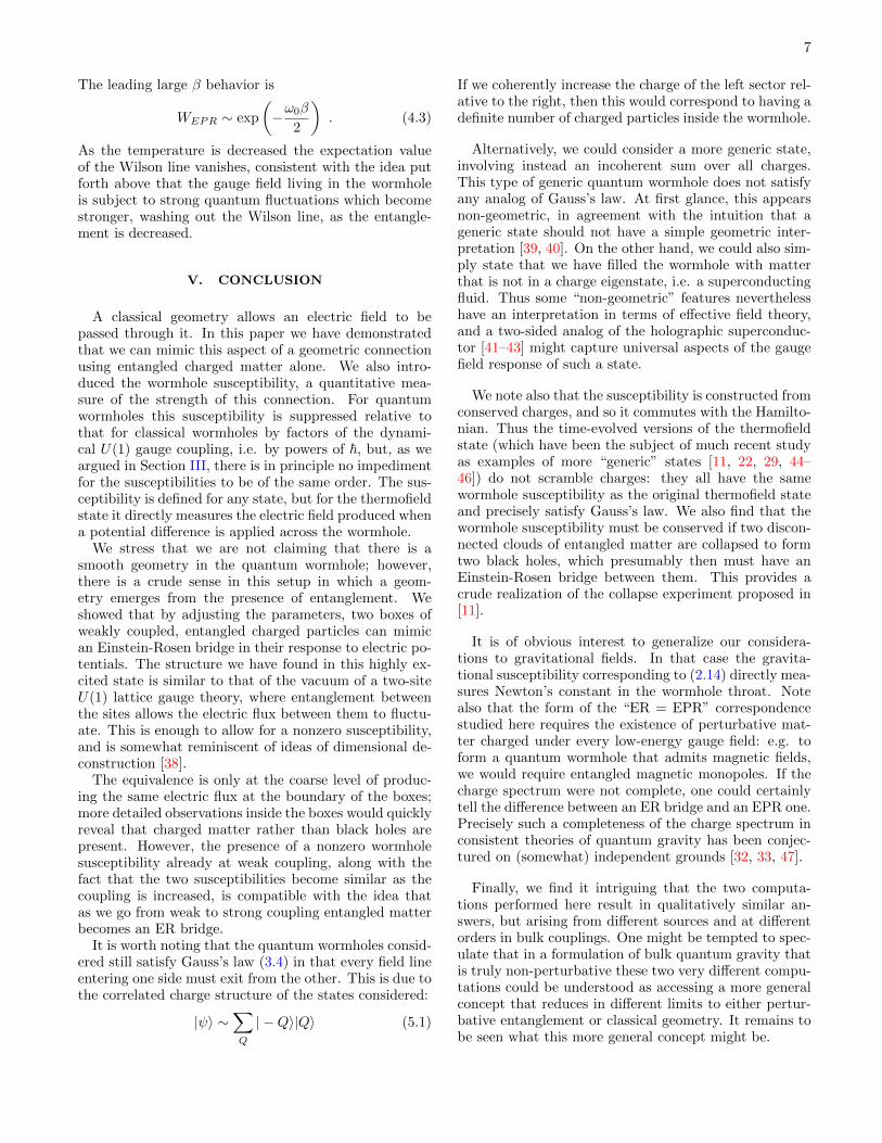
V. CONCLUSION

A classical geometry allows an electric field to bepassed through it. In this paper we have demonstratedthat we can mimic this aspect of a geometric connectionusing entangled charged matter alone. We also intro-duced the wormhole susceptibility, a quantitative mea-sure of the strength of this connection. For quantumwormholes this susceptibility is suppressed relative tothat for classical wormholes by factors of the dynami-cal U(1) gauge coupling, i.e. by powers of ~, but, as weargued in Section III, there is in principle no impedimentfor the susceptibilities to be of the same order. The sus-ceptibility is defined for any state, but for the thermofieldstate it directly measures the electric field produced whena potential difference is applied across the wormhole.

We stress that we are not claiming that there is asmooth geometry in the quantum wormhole; however,there is a crude sense in this setup in which a geom-etry emerges from the presence of entanglement. Weshowed that by adjusting the parameters, two boxes ofweakly coupled, entangled charged particles can mimican Einstein-Rosen bridge in their response to electric po-tentials. The structure we have found in this highly ex-cited state is similar to that of the vacuum of a two-siteU(1) lattice gauge theory, where entanglement betweenthe sites allows the electric flux between them to fluctu-ate. This is enough to allow for a nonzero susceptibility,and is somewhat reminiscent of ideas of dimensional de-construction [38].

The equivalence is only at the coarse level of produc-ing the same electric flux at the boundary of the boxes;more detailed observations inside the boxes would quicklyreveal that charged matter rather than black holes arepresent. However, the presence of a nonzero wormholesusceptibility already at weak coupling, along with thefact that the two susceptibilities become similar as thecoupling is increased, is compatible with the idea thatas we go from weak to strong coupling entangled matterbecomes an ER bridge.

It is worth noting that the quantum wormholes consid-ered still satisfy Gauss’s law (3.4) in that every field lineentering one side must exit from the other. This is due tothe correlated charge structure of the states considered:

|ψ〉 ∼∑Q

| −Q〉|Q〉 (5.1)

If we coherently increase the charge of the left sector rel-ative to the right, then this would correspond to having adefinite number of charged particles inside the wormhole.

Alternatively, we could consider a more generic state,involving instead an incoherent sum over all charges.This type of generic quantum wormhole does not satisfyany analog of Gauss’s law. At first glance, this appearsnon-geometric, in agreement with the intuition that ageneric state should not have a simple geometric inter-pretation [39, 40]. On the other hand, we could also sim-ply state that we have filled the wormhole with matterthat is not in a charge eigenstate, i.e. a superconductingfluid. Thus some “non-geometric” features neverthelesshave an interpretation in terms of effective field theory,and a two-sided analog of the holographic superconduc-tor [41–43] might capture universal aspects of the gaugefield response of such a state.

We note also that the susceptibility is constructed fromconserved charges, and so it commutes with the Hamilto-nian. Thus the time-evolved versions of the thermofieldstate (which have been the subject of much recent studyas examples of more “generic” states [11, 22, 29, 44–46]) do not scramble charges: they all have the samewormhole susceptibility as the original thermofield stateand precisely satisfy Gauss’s law. We also find that thewormhole susceptibility must be conserved if two discon-nected clouds of entangled matter are collapsed to formtwo black holes, which presumably then must have anEinstein-Rosen bridge between them. This provides acrude realization of the collapse experiment proposed in[11].

It is of obvious interest to generalize our considera-tions to gravitational fields. In that case the gravita-tional susceptibility corresponding to (2.14) directly mea-sures Newton’s constant in the wormhole throat. Notealso that the form of the “ER = EPR” correspondencestudied here requires the existence of perturbative mat-ter charged under every low-energy gauge field: e.g. toform a quantum wormhole that admits magnetic fields,we would require entangled magnetic monopoles. If thecharge spectrum were not complete, one could certainlytell the difference between an ER bridge and an EPR one.Precisely such a completeness of the charge spectrum inconsistent theories of quantum gravity has been conjec-tured on (somewhat) independent grounds [32, 33, 47].

Finally, we find it intriguing that the two computa-tions performed here result in qualitatively similar an-swers, but arising from different sources and at differentorders in bulk couplings. One might be tempted to spec-ulate that in a formulation of bulk quantum gravity thatis truly non-perturbative these two very different compu-tations could be understood as accessing a more generalconcept that reduces in different limits to either pertur-bative entanglement or classical geometry. It remains tobe seen what this more general concept might be.

8

ACKNOWLEDGMENTS

It is our pleasure to acknowledge helpful discussionswith J. Camps, N. Engelhardt, D. Harlow, D. Hofman,P. Kraus, P. de Lange, L. Kabir, M. Lippert, A. Puhm, J.Santos, G. Sarosi, J. Sully, L. Susskind, D. Tong, L. Thor-lacius, and B. Way. This work was supported by the NSFgrant DGE-0707424, the University of Amsterdam, theNetherlands Organisation for Scientific Research (NWO),and the D-ITP consortium, a program of the NWO thatis funded by the Dutch Ministry of Education, Cultureand Science (OCW). N.I. would like to acknowledge thehospitality of DAMTP at the University of Cambridgewhile this work was in progress.

Appendix A: Charged scalar field computations

0.5 1.0 1.5 2.0 2.5mΒ

-6

-4

-2

2

log YΦL HΦR L† ]

FIG. 6. Numerical evaluation of logarithm of 〈φL(0)φ†R(0)〉,which contributes the interesting dependence of the Wilsonline (4.2). From bottom moving upwards, curves correspondto ma = 1, 1.5, 2. Dashed line corresponds to asymptotic

behavior for ma = 1 of exp(−ω0

2β

)with ω0 the lowest single-

particle energy level.

Here we present some details of the charged scalar fieldcomputations presented in the main text. Similar resultswould be obtained for essentially any system in any ge-ometry, but for concreteness we present the precise for-mulas for the charged scalar field in a spherical box. Therelevant part of the action is

Sφ = −∫d4x

(|Dφ|2 +m2|φ|2

)(A1)

The scalar field is confined to a spherical box of radiusa with Dirichlet boundary conditions φ(r = a) = 0. Wefirst compute the single-particle energy levels.

Expanding the field in spherical harmonics as φ =∑lmp φlp(r)e

−iωt Ylm(θ, φ) we find the mode equation

for φlp(r) to be

1

r2∂r(r2∂rφlp(r)

)− l(l + 1)

r2φlp(r) = (m2 − ω2)φlp(r),

(A2)Here p is a radial quantum number and l is angular mo-mentum as usual. The normalizable solutions to the ra-dial wave equation are spherical Bessel functions of order

l:

φlp(r) = clpjs(l, λlpr) clp =2√a3π

(Jl+ 3

2(λlpa)

)−1

(A3)The normalization clp has been picked such that∑

p

φlp(r)φlp(r′) =

δ(r − r′)r2

(A4)

In clp, Jν(x) is an ordinary Bessel function of the firstkind. Imposing the Dirichlet boundary condition fixesλp =

xlp

a , where xlp is the p-th zero of the l-th sphericalBessel function. This determines the energy levels to be

ωlp =

√m2 +

(xlpa

)2

, (A5)

We are now interested in computing the charge suscepti-bility at finite temperature T and chemical potential µ.From elementary statistical mechanics we have the usualexpression for the charge

〈Q〉 = q∑lp

(2l + 1)

(1

1− eβ(ωlp+qµ)− 1

1− eβ(ωlp−qµ)

),

(A6)where we have included the degeneracy factor (2l + 1).Linearizing this in µ we obtain (3.5), where it is under-stood that the sum over single-particle states there in-cludes a sum over angular momentum eigenstates:

∑n →∑

lp(2l + 1).Next we compute the correlation function

〈φ†L(0)φR(0)〉 across the two sides of the thermofieldstate (3.3) (with µ → 0). The fastest way to computethis is to note that the two sides of the thermofield statecan be understood as being connected by Euclidean timeevolution through β

2 . Thus the mixed correlator can becalculated by computing the usual Euclidean correlatorbetween two points separated by β

2 in Euclidean time(see e.g. [1]). If the single-particle energy levels aregiven by ωpl, then the Euclidean correlator between twogeneral points is

G(τ, r, θ, φ; τ ′, r′, θ′, φ′) =∑lmp

1

2ωlp

cosh(ωlp

(τ − τ ′ − β

2

))sinh

(βωlp

2

) ×

φpl(r)φpl(r′)Ylm(θ, φ)Y ∗lm(θ′, φ′), (A7)

where in this expression the normalization of the modefunctions (A4) is important.

For our application to the Wilson line in (4.2) we care

about the specific case τ − τ ′ = β2 and r = r′ = 0. The

spherical Bessel functions with nonzero angular momen-tum l 6= 0 all vanish at the origin r = 0. Thus the sum isonly over the l = 0 modes. The result of performing thissum numerically is shown in Figure 6, but it is easy to seethat at small temperatures the answer will be dominatedby the lowest energy level and is:

〈φL(0)†φR(0)〉 ∼ exp

(−ω0β

2

). (A8)

9

[1] J. M. Maldacena, “Eternal black holes in anti-deSitter,” JHEP 0304 (2003) 021, arXiv:hep-th/0106112[hep-th].

[2] S. Ryu and T. Takayanagi, “Aspects of HolographicEntanglement Entropy,” JHEP 0608 (2006) 045,arXiv:hep-th/0605073 [hep-th].

[3] S. Ryu and T. Takayanagi, “Holographic derivation ofentanglement entropy from AdS/CFT,” Phys.Rev.Lett.96 (2006) 181602, arXiv:hep-th/0603001 [hep-th].

[4] V. E. Hubeny, M. Rangamani, and T. Takayanagi, “ACovariant holographic entanglement entropy proposal,”JHEP 0707 (2007) 062, arXiv:0705.0016 [hep-th].

[5] B. Swingle, “Entanglement renormalization andholography,” Phys. Rev. D 86 (Sep, 2012) 065007,arXiv:0905.1317 [cond-mat].

[6] T. Faulkner, M. Guica, T. Hartman, R. C. Myers, andM. Van Raamsdonk, “Gravitation from Entanglementin Holographic CFTs,” JHEP 1403 (2014) 051,arXiv:1312.7856 [hep-th].

[7] N. Lashkari, M. B. McDermott, andM. Van Raamsdonk, “Gravitational dynamics fromentanglement ’thermodynamics’,” JHEP 1404 (2014)195, arXiv:1308.3716 [hep-th].

[8] M. Van Raamsdonk, “Comments on quantum gravityand entanglement,” arXiv:0907.2939 [hep-th].

[9] M. Van Raamsdonk, “Building up spacetime withquantum entanglement,” Gen.Rel.Grav. 42 (2010)2323–2329, arXiv:1005.3035 [hep-th].

[10] B. Swingle and M. Van Raamsdonk, “Universality ofGravity from Entanglement,” arXiv:1405.2933

[hep-th].[11] J. Maldacena and L. Susskind, “Cool horizons for

entangled black holes,” Fortsch.Phys. 61 (2013)781–811, arXiv:1306.0533 [hep-th].

[12] A. Einstein, B. Podolsky, and N. Rosen, “Can quantummechanical description of physical reality be consideredcomplete?,” Phys.Rev. 47 (1935) 777–780.

[13] A. Einstein and N. Rosen, “The Particle Problem in theGeneral Theory of Relativity,” Phys.Rev. 48 (1935)73–77.

[14] L. Susskind, “New Concepts for Old Black Holes,”arXiv:1311.3335 [hep-th].

[15] M. Chernicoff, A. Gijosa, and J. F. Pedraza,“Holographic EPR Pairs, Wormholes and Radiation,”JHEP 1310 (2013) 211, arXiv:1308.3695 [hep-th].

[16] L. Susskind, “Butterflies on the Stretched Horizon,”arXiv:1311.7379 [hep-th].

[17] L. Susskind, “Computational Complexity and BlackHole Horizons,” arXiv:1402.5674 [hep-th].

[18] L. Susskind, “Addendum to Computational Complexityand Black Hole Horizons,” arXiv:1403.5695 [hep-th].

[19] D. Stanford and L. Susskind, “Complexity and ShockWave Geometries,” Phys.Rev. D90 no. 12, (2014)126007, arXiv:1406.2678 [hep-th].

[20] L. Susskind and Y. Zhao, “Switchbacks and the Bridgeto Nowhere,” arXiv:1408.2823 [hep-th].

[21] L. Susskind, “ER=EPR, GHZ, and the Consistency ofQuantum Measurements,” arXiv:1412.8483 [hep-th].

[22] D. A. Roberts, D. Stanford, and L. Susskind, “Localizedshocks,” JHEP 1503 (2015) 051, arXiv:1409.8180[hep-th].

[23] L. Susskind, “Entanglement is not Enough,”arXiv:1411.0690 [hep-th].

[24] K. Jensen and A. Karch, “Holographic Dual of anEinstein-Podolsky-Rosen Pair has a Wormhole,”Phys.Rev.Lett. 111 no. 21, (2013) 211602,arXiv:1307.1132 [hep-th].

[25] J. Sonner, “Holographic Schwinger Effect and theGeometry of Entanglement,” Phys.Rev.Lett. 111 no. 21,(2013) 211603, arXiv:1307.6850 [hep-th].

[26] K. Jensen and J. Sonner, “Wormholes andentanglement in holography,” Int.J.Mod.Phys. D23no. 12, (2014) 1442003, arXiv:1405.4817 [hep-th].

[27] K. Jensen, A. Karch, and B. Robinson, “Holographicdual of a Hawking pair has a wormhole,” Phys.Rev.D90 no. 6, (2014) 064019, arXiv:1405.2065 [hep-th].

[28] H. Gharibyan and R. F. Penna, “Are entangled particlesconnected by wormholes? Evidence for the ER=EPRconjecture from entropy inequalities,” Phys.Rev. D89no. 6, (2014) 066001, arXiv:1308.0289 [hep-th].

[29] K. Papadodimas and S. Raju, “Comments on theNecessity and Implications of State-Dependence in theBlack Hole Interior,” arXiv:1503.08825 [hep-th].

[30] D. Garfinkle and A. Strominger, “Semiclassical Wheelerwormhole production,” Phys.Lett. B256 (1991)146–149.

[31] C. W. Misner and J. A. Wheeler, “Classical physics asgeometry: Gravitation, electromagnetism, unquantizedcharge, and mass as properties of curved empty space,”Annals Phys. 2 (1957) 525–603.

[32] N. Arkani-Hamed, L. Motl, A. Nicolis, and C. Vafa,“The String landscape, black holes and gravity as theweakest force,” JHEP 0706 (2007) 060,arXiv:hep-th/0601001 [hep-th].

[33] T. Banks and N. Seiberg, “Symmetries and Strings inField Theory and Gravity,” Phys.Rev. D83 (2011)084019, arXiv:1011.5120 [hep-th].

[34] W. Israel, “Thermo field dynamics of black holes,”Phys.Lett. A57 (1976) 107–110.

[35] T. Andrade, S. Fischetti, D. Marolf, S. F. Ross, andM. Rozali, “Entanglement and correlations nearextremality: CFTs dual to Reissner-Nordstrm AdS5,”JHEP 1404 (2014) 023, arXiv:1312.2839 [hep-th].

[36] S. Leichenauer, “Disrupting Entanglement of BlackHoles,” Phys.Rev. D90 no. 4, (2014) 046009,arXiv:1405.7365 [hep-th].

[37] D. Harlow, “Aspects of the Papadodimas-Raju Proposalfor the Black Hole Interior,” JHEP 1411 (2014) 055,arXiv:1405.1995 [hep-th].

[38] N. Arkani-Hamed, A. G. Cohen, and H. Georgi,“(De)constructing dimensions,” Phys.Rev.Lett. 86(2001) 4757–4761, arXiv:hep-th/0104005 [hep-th].

[39] D. Marolf and J. Polchinski, “Gauge/Gravity Dualityand the Black Hole Interior,” Phys.Rev.Lett. 111 (2013)171301, arXiv:1307.4706 [hep-th].

[40] V. Balasubramanian, M. Berkooz, S. F. Ross, and

10

J. Simon, “Black Holes, Entanglement and RandomMatrices,” Class.Quant.Grav. 31 (2014) 185009,arXiv:1404.6198 [hep-th].

[41] S. S. Gubser, “Breaking an Abelian gauge symmetrynear a black hole horizon,” Phys.Rev. D78 (2008)065034, arXiv:0801.2977 [hep-th].

[42] S. A. Hartnoll, C. P. Herzog, and G. T. Horowitz,“Building a Holographic Superconductor,”Phys.Rev.Lett. 101 (2008) 031601, arXiv:0803.3295[hep-th].

[43] S. A. Hartnoll, C. P. Herzog, and G. T. Horowitz,“Holographic Superconductors,” JHEP 0812 (2008)

015, arXiv:0810.1563 [hep-th].[44] T. Hartman and J. Maldacena, “Time Evolution of

Entanglement Entropy from Black Hole Interiors,”JHEP 1305 (2013) 014, arXiv:1303.1080 [hep-th].

[45] K. Papadodimas and S. Raju, “Local Operators in theEternal Black Hole,” arXiv:1502.06692 [hep-th].

[46] S. H. Shenker and D. Stanford, “Black holes and thebutterfly effect,” JHEP 1403 (2014) 067,arXiv:1306.0622 [hep-th].

[47] J. Polchinski, “Monopoles, duality, and string theory,”Int.J.Mod.Phys. A19S1 (2004) 145–156,arXiv:hep-th/0304042 [hep-th].