IHCP TECHNIQUE BASED ON GREEN’S FUNCTIONS AND …

Proceedings of ENCIT 2010 13th Brazilian Congress of Thermal Sciences and Engineering

Copyright © 2010 by ABCM December 05-10, 2010, Uberlandia, MG, Brazil

IHCP TECHNIQUE BASED ON GREEN’S FUNCTIONS AND DYNAMIC

OBSERVERS APLIED TO ORTHOGONAL CUTTING

Tostes, A. A. M., [email protected]

Sousa, P. F. B., [email protected]

Guimarães, G., [email protected] School of Mechanical Engineering, Federal University of Uberlândia, Av. João Naves de Ávila, 2131, CEP 38400-902, Uberlândia, M.G., Brazil. Telephone: +55 34 3239-4147

Abstract. The temperature fields generated in the cutting processes is subject of much research. The studies of these

thermal fields in machining are very important for the development of new technologies aimed to increase tool live and

to reduce production costs. Cutting temperatures have strongly influenced both the tool life and the metallurgical state

of machined surfaces. Since the direct temperature measurements at the tool-piece interface are very complex this

work proposes the estimation of the temperature and the heat flux at the tool-piece interface using the inverse heat

conduction problem technique. The aim of the present paper is to develop a three-dimensional inverse algorithm in

transient conditions for heat flux and machining temperature estimation. The thermal model is obtained by the

numerical solution of the transient 3D heat diffusion equation that considers both the tool and tool holder assembly.

The thermal model is developed by using the finite elements method in ANSYS®

code with a mesh of 149.150 elements

and SOLID70 element as shown . The inverse solution is performed by using the technique based on Green’s functions

and dynamic observers. Simulated cases were investigated and presented excellent results.

Keywords: Heat Flux, Machining processes, FEM, IHCP, Dynamic Observer, Green's Function

1. INTRODUCTION

Temperature knowledge at the cutting interface during a machining process is very important. Cutting temperatures have strongly influenced both the tool life and the metallurgical state of machined surfaces. Several studies can be largely found at the literature regarding this subject.

Numerical simulation methods applied to machining process have been increasing during the last decade. Nowadays numerical simulation techniques are widely required to predict and optimize machining processes, combining cutting parameters in order to obtain better machined surfaces, or even to reduce temperature during a machining process. Several authors have proposed numerical and experimental techniques trying to predict temperature field at the tool and piece during machining process. Since the direct temperature measurements at the tool-piece interface are very complex the inverse solution represents a good approach.

Using numerical analysis Jen & Gutierrez (2000) investigated the tool temperature distribution considering different thermal properties. For this purpose the authors developed a three-dimensional transient thermal model with a FEM (Finite Element Method) formulation. For the solution the authors considered a known heat flux at the cutting interface and neglected convection effects and contact resistance. In this study the tool geometry influence under the temperature was evaluated. J. Yvonnet et al (2006) proposed an inverse technique to indentify the generated heat flux at the cutting interface and the heat transfer coefficient between tool and the environment during a typical orthogonal cutting process.

Carvalho (2006) developed a three-dimensional numerical model of a tool-holder set using Finite Difference Method. The heat flux at the cutting interface was estimated by using golden section that is an optimization technique with polynomial approach. The author used this procedure to estimated heat flux generated during a turning process. It was possible to analyze the high temperature gradients and its bad effects on tool life. The technique is suitable to solve the inverse problem but presents some restriction with the time step.

Sousa(2006) proposed an inverse technique based on Dynamic observer and Green's function to estimate heat flux generated at the cutting interface during a drilling process. The direct model consists on a three-dimensional piece been drilled, the model was developed using Finite Volume Method. In this case the author was focused on the resulting thermal field at the piece. The inverse technique was applied with success to solve inverse drilling problem. The study showed that the temperature and heat flux at the tool-piece interface during a drilling process can be estimated if a suitable experimental apparatus was designed avoiding problems of sensitivity. Sousa has shown that the inverse technique is very simple to be implemented and has a great flexibility since it is possible to build the direct problem using any method or computational language.

This work proposes a thermal analysis of a turning process. The tool-holder set thermal field is here identified by using FEM (Finite Elements Method) and the inverse technique is based on Dynamic Observers and Green's function. The main goal is to obtain the tool-holder set temperature distribution by estimating the heat flux at interface work-piece. Simulated cases were investigated and the inverse technique is ready to be applied in a real cutting situation.



2. FUNDAMENTALS

Direct model that was solved using FEM is represented by a tool-holder set as shows Fig. 1.

2.1. Thermal model: direct problem

The direct problem is represented by a tool -holder set as shown in Fig. 1. It is considered here a cemented carbide

tool and a titanium holder. Thermal properties for the holder and tool are shown in Table 1. The thermal model geometry was built using Auto-Cad® in order to obtain the mesh to be used in the FEM

(ANSYS®). Heat flux, q''(t), that appears during a machining process is generated in the contact area, S1 as represented

in Fig. 1. Thermal model also consider convection effects around the tool-holder set.

Figure 1. Three-dimensional thermal machining problem The thermal model is obtained by the numerical solution of the transient and three-dimensional heat diffusion

equation, that can be described by

( ) ( ) ( )t

tzyxT

z

tzyxT

y

tzyxT

x

tzyxT

∂∂

=∂

∂+

∂∂

+∂

∂ ),,,(1),,,(),,,(),,,(2

2

22

2

α

(1)

In the region R (0 < x < a, 0 < y < b, 0 < z < c) and t> 0, subjected to the boundary conditions in the cutting

interface:

( )),(),0,,(

,0,,111 yyyxxxSontyxq

z

tyxTk oo ≤≤≤≤=

∂∂

− (2)

[ ] ),(),0,,(),0,,(

112 byyaxxSonTtyxThz

tyxk ≤≤≤≤−=

∂∂

− ∞ (3)

[ ] ),(),0,,(),0,,(

3 byydxaSonTtyxThz

tyxk o ≤≤≤≤−=

∂∂

− ∞ (4)

[ ] ),(),0,,(),0,,(

4 byydaxxSonTtyxThz

tyxk oo ≤≤+≤≤−=

∂∂

− ∞ (5)

( )[ ] c)zza,x(xSonTtz,x,0,Th

y

t)z,(x,0,k oo5 ≤≤≤≤−=

∂∂

∞ (6)

( )[ ] c)zzd,x(aSonTtz,x,0,Th

y

t)z,(x,0,k 16 ≤≤≤≤−=

∂∂

∞

(7)

( )[ ] ),(,,,),,,(

7 czzaxxSonTtzbxThy

tzbxk oo ≤≤≤≤−=

∂∂

− ∞ (8)

.S1

q”(t)



( )[ ] ),(,,,),,,(

18 czzdxaSonTtzbxThy

tzbxk ≤≤≤≤−=

∂∂

− ∞

(9)

( )[ ] ),(9,,,0),,,0(

czozbyoySonTtzyThx

tzyk ≤≤≤≤∞−=

∂∂ (10)

( )[ ] ),(10,,,),,,(

czozdbxoySonTtzyaThx

tzyak ≤≤+≤≤∞−=

∂

∂− (11)

( )[ ] ),(11,,,),,,(

czo

zbyo

ySonTtzydaThx

tzydak ≤≤≤≤∞−+=

∂

+∂− (12)

T(x,y,z,0)=T0 for t>0 in the region R.

In the Equation 1 where Si represents the different surfaces to be considered in thermal model and can be better

identified in section 3 (Fig. 5). If the value of the heat flux, q”(x, y,0, t), is known, the Eq. (1) represent the direct problem related to the inverse problem studied.

The thermal model has considered that the thermal properties of both tool and holder materials are constant. The

respective values are shown in Tab. 1.

Table 1. Thermal Properties of workpiece (cemented carbide) and tool holder (titanium).

Materials k[W/mK] ρ[kg/m^3] cp[J/kgK] ε[J/Km2s1/2]

titanium 21 4650 645 7936,26

cemented carbide 43,1 14600 200 11218,4

2.2. Inverse Technique

The inverse problem solution technique based on Green’s functions and dynamic observers with global transfer Function, Sousa (2009) can be divided in two distinct steps: i) obtaining of the transfer function model GH; ii) obtaining of the heat transfer functions GQ and GN and the building algorithm identification. The transfer function model, GH, is obtained from the equivalent dynamic systems theory and using Green’s functions. The GQ and GN are obtained by following the procedure presented by Blum and Marquardt (1997).

Transfer Function Model identification (GH). The solution of Eq. (13) can be given in terms of Green’s function

as by Beck et al. (1992)

( ) ( ) ( )[ ]dτt

0τ1

qt/τz,y,x,H

Gtz,y,x,T ∫=

= τ (13)

where

∫ ∫=

+=−h

x

0

hz

0

dz'dx'

Hyy'

τ),z',y',t/x'z,y,(x,H

Gk

ατ)tz,y,(x,

HG (14)

and ),,,( τ−tzyxG represents the Green’s function of the thermal problem given by Eq.(14).

The Green’s function is available for the homogeneous version associated with the problem defined by Eq. (1). Although the analytical Green’s function is available and exists, Beck et al. (1992), it will not be used in this work. By the contrary, the solution of the problem defined by Eq. (1) will be performed numerically using finite element methods.

Equation (14) reveals that an equivalent thermal model can be associated with a dynamic model. It means, a response of the input/output system can be associated to Eq. (15) in the Laplace domain as the convolution product (Özisik, 1993)



( ) )(1qτ)tz,y,(x,HGtz,y,x,T τ∗−= (15)

This dynamic system can be represented as shown in Fig. (2). Equation (15) can also be evaluated in the Laplace domain as a single product

( ) (s)

1qs)z,y,(x,

HGsz,y,x,T = (16)

X(t) = q(t)

Y i(t) = T (xi,yi,zi,t)

),,,( τ−tzyxGH

Figure 2. Dynamic thermal model system

The complete GH identification is obtained using an auxiliary problem. The heat transfer function ),,,( szyxGH

can, then, be obtained through the auxiliary problem which is a homogenous version of the problem defined by Eq. (13) for the same region with a zero initial temperature and unit impulsive source located at the region of the original heating. It means, the auxiliary thermal problem can be described as.

Similarly, the auxiliary thermal problem solution can be derived using Green function and the convolution properties as

( ) 1)τt,z,y,(xHGt,z,y,xT ∗+−++++=+++++ (17)

The Laplace transform of 1 is

[ ]s

L1

1 = , then (18)

( )s

1s),z,y,(xHGs,z,y,xT +++=++++ (19)

If the dynamic system is linear, invariant, and physically invariable, the response function ),,,( szyxGH is the

same, independently of the pairs input/output and can be obtained by

( )sz,y,x,Tss)z,y,(x,GH+= (20)

In order to complete the ),,,( szyxGH identification, the ),,,( szyxT + must be obtained at a specific position ri =

(xi, yi, zi).

A simple and efficient procedure is proposed here to obtain ),( srT i+ : if Eq. (20) represents a cross correlation

function of the two functions of stationary random process s and ( )szyT ,,,x+ , then ),,,( szyxGH will be

independent of the absolute time t and will depend only on the time separation ta.

In this case, provided that the function ),( srT i+ can be fitted by a polynomials function in the sampled interval [0,

ta] as

( ) Λ+++=+ 3t3a

2t2at1at,irT (21)

where ai are the polynomial coefficients. Then, taking the Laplace transform of Eq. (21) gives



( ) n1)s(n

na

46s

4a

32s

3a

2s

2a

s

1as,irT

−+++++=+ Λ (22)

Thus, from Eq. (20) GH can be written as

( )

+++=+=

ns

na

2s

2a

s

1ass,irTss),i(rHG Λ (23)

or +++++= Λ3

4

2

321iH

6s

a

2s

a

s

aas),(rG (24)

It can be observed that from the theory of partial fractions, if ),( srG iH is expressible in partial fractions as in Eq.

(24) its inversion is readily obtained by using the Laplace transform table. An advantage of this procedure is that the same procedure can be used indistinctly by one, two or three-dimensional models, provided the only active boundary condition is the unknown heat source.

The Global Transfer function is obtained using more than one thermocouple information. Figure 3 presents a single-input/two-output system. It means this figure shows an equivalent dynamic system to a thermal problem given by Fig. 1 considering two thermocouples for different positions (1, 2). It is assumed here that noise terms n1(t) and n2(t) are uncorrelated with each other and with the input signal q(t).

GH1(f)

GH2(f)

q(t)

θ1(t)

Y

∑

∑

n1(t)

n2(t)

θ2(t)

θM1(t)

θM2(t)

Figure 3. Single-input/two-output system.

In this case Eq.(13) gives

( ) ∫=

−=t

jHj dqtyGty

0ii )(),,x(,,x

τ

τττθ (25)

or in Laplace domain

( ) )(),,x(,,x 1111 sqsyGsy H=θ (26)

( ) )(),,x(,,x 2222 sqsyGsy H=θ (27)

Adding Eq.(26) to Eq.(27)

[ ] )()()( 2121 sqsGsG HH +=+θθ (28)

As Equation (28) has a similar representation of Eq. (16) the same estimators can be used to represent the single-

input/two-output system. The only change that must be made is to consider the sum of temperature and the sum of heat transfer function in the system. As mentioned, the use of more than two thermocouples is immediate.

At this point, the GQ and GN functions need to be obtained in order to complete the inverse algorithm.

Obtaining of estimators Transfer Functions GQ and GN. The thermal model can be represented by a dynamic system given by a block diagram shown in Fig. 4 (Blum and Marquardt, 1997):



GH N

Gc

ĜH

+

+ +

q̂

q̂

Mθ̂

θM

θM

-

?=q θ

Figure 4. Frequency-domain block diagram.

It can be observed from the block diagram that: i) the unknown heat flux q(s) is applied to the conductor (reference model), GH, and results in a measurement signal θM

corrupted by noise N,

NqGN HM +=+= θθ (29)

ii) The estimate value q̂ is computed from the output data Mθ . Thus, the estimator can be represented in a closed-loop

transfer function of the feedback loop (Fig. 4) as

M

HC

C θGG1

Gq

+=ˆ (30)

that characterizes the behavior of the solution algorithm. Substituting Eq. (29) in Eq. (30) we obtain:

NGG1

Gq

GG1

GGq

Hc

C

Hc

HC

++

+=ˆ (31)

or

NGqGq NQ +=ˆ (32)

where

Hc

HCQ

GG

GGG

+=

1and

Hc

C

H

QN

GG1

G

G

GG

+== (33)

The transfer function GQ is chosen to have the behavior of type I chebychev filter and GN is identified by Eq. (33) provided that GH is obtained. Thus, from Eq. (30) the resulting algorithm can then be given by

( ) ( ) ( )ssGsq MN θ×=ˆ (34)

It can be observed in Eq. (33) that if the algorithm estimates the heat flux correctly, GQ is equal to unity, GQ = 1, and the frequency w is within the pass band. In this case, the noise transfer function GN is equal to the inverse transfer function of the heat conductor (GH

-1). According to Blum and Marquardt the observer is essentially an on-line scheme. In this case, estimation of the heat flux at the current time step is based on current and past temperature measurements only. In this case, any on-line estimator involves a phase shift or lag. To remove this lag Blum and Marquardt proposed a filtering procedure that can be resumed in the use of two discrete-time difference equations

)()()(10

ikqaikYbkqnn n

i

iM

n

i

i −−−= ∑∑==

(35)

and



)(ˆ)()(ˆ10

ikqaikqbkqnn n

i

i

n

i

i −−−= ∑∑==

(36)

The coefficients ai and bi that appear in Eqs. (35) and (36) are obtained using Eq. (33). In this case, the inverse

procedure is concluded with the ),,( syxGH identification.

3. RESULTS AND DISCUSSION

The inverse technique based on Green's functions and dynamic observers with global transfer function is applied to solve a simulated case. Simulated tests are important to evaluate the inverse technique algorithm and to investigate possible problem of sensitivity. The great advantage of this procedure, for example, is to avoid additional complications, such as biases in the direct problem and to use the results to design the best experimental apparatus defining important variable as sensor locations or time during of the experiment. Simulated data can also be used to establish the sensitivity of the problem and to anticipate possible inverse estimation problems.

This section presents a simulated test case considering a tool-holder set with a cemented carbide tool and titanium holder which thermal properties are presented in Tab. 1.

Simulated temperature data distributions for the direct problem are generated using the solution of Eq. (1). considering a known heat flux evolution q’’(t). Random errors are then added to these temperatures. The temperatures with error are then used in the inverse algorithm to reconstruct the imposed heat flux. The experimental simulated temperatures are calculated from the following equation:

jtLTtLY ε+= ),(),( (37)

where jε is a random number. The parameter jε assumes values of 0, and within ± 1°C .

3.1. Simulated test

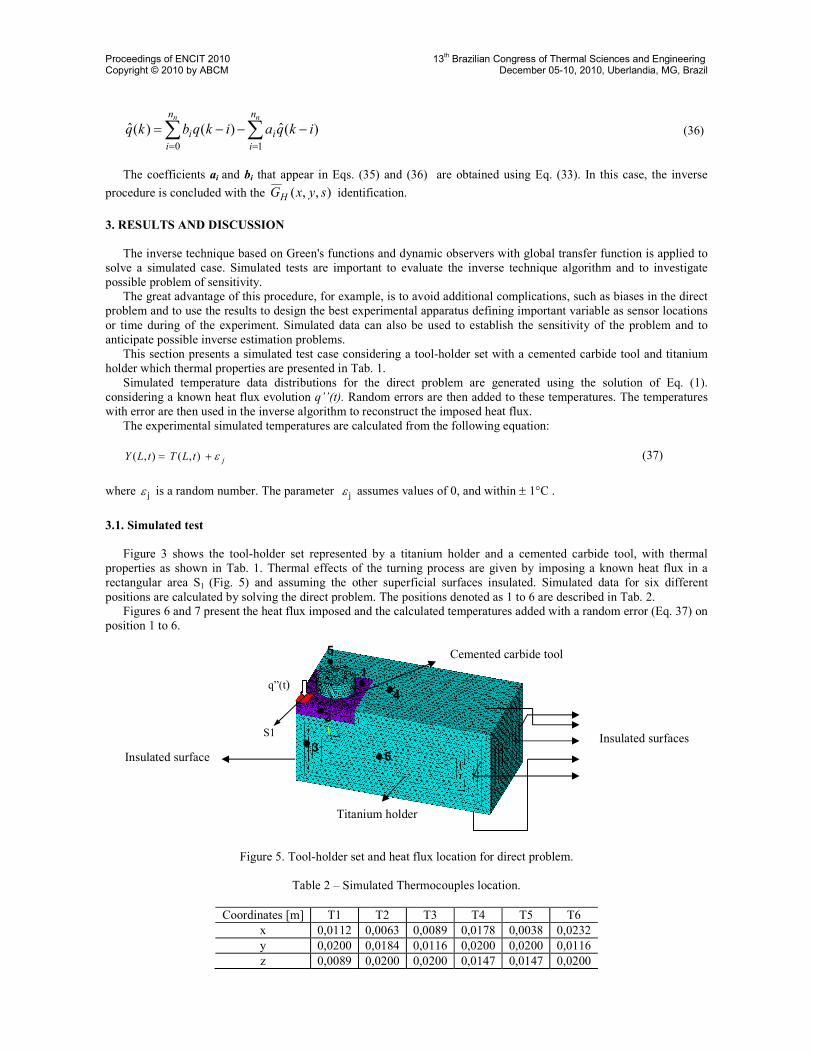
Figure 3 shows the tool-holder set represented by a titanium holder and a cemented carbide tool, with thermal properties as shown in Tab. 1. Thermal effects of the turning process are given by imposing a known heat flux in a rectangular area S1 (Fig. 5) and assuming the other superficial surfaces insulated. Simulated data for six different positions are calculated by solving the direct problem. The positions denoted as 1 to 6 are described in Tab. 2.

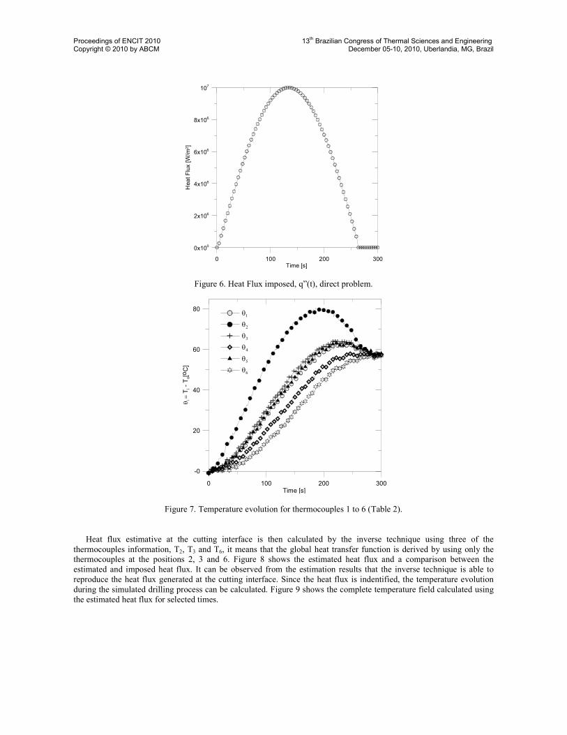
Figures 6 and 7 present the heat flux imposed and the calculated temperatures added with a random error (Eq. 37) on position 1 to 6.

Figure 5. Tool-holder set and heat flux location for direct problem.

Table 2 – Simulated Thermocouples location.

Coordinates [m] T1 T2 T3 T4 T5 T6 x 0,0112 0,0063 0,0089 0,0178 0,0038 0,0232 y 0,0200 0,0184 0,0116 0,0200 0,0200 0,0116 z 0,0089 0,0200 0,0200 0,0147 0,0147 0,0200

S1

q”(t)

.

Titanium holder

Cemented carbide tool

Insulated surfaces

1

4

5

6 3

2

Insulated surface



0 100 200 300Time [s]

0x100

2x106

4x106

6x106

8x106

107

Heat Flux [W/m

2]

Figure 6. Heat Flux imposed, q”(t), direct problem.

0 100 200 300Time [s]

-0

20

40

60

80

θ i =

Ti - T

o[oC]

θ1

θ2

θ3

θ4

θ5

θ6

Figure 7. Temperature evolution for thermocouples 1 to 6 (Table 2).

Heat flux estimative at the cutting interface is then calculated by the inverse technique using three of the

thermocouples information, T2, T3 and T6, it means that the global heat transfer function is derived by using only the thermocouples at the positions 2, 3 and 6. Figure 8 shows the estimated heat flux and a comparison between the estimated and imposed heat flux. It can be observed from the estimation results that the inverse technique is able to reproduce the heat flux generated at the cutting interface. Since the heat flux is indentified, the temperature evolution during the simulated drilling process can be calculated. Figure 9 shows the complete temperature field calculated using the estimated heat flux for selected times.



0 100 200 300Time [s]

-0x100

2x106

4x106

6x106

8x106

107

Heat Flux [W/m2]

Estimated Heat Flux

Imposed Heat Flux

Figure 8. Estimated heat flux versus imposed heat flux

Figure 9. Resulting temperature field during a machining process at different elapsed machining times.

Temperature control is important to prevent piece and tool damage due to the excessive temperature. Since heat flux at the cutting interface has been reconstructed it is possible to estimate the maximum temperature at the piece solving the direct problem.

Figure 10 shows a comparison between the calculated and the measured temperatures for thermocouples 1 and 4. It is observed a good accordance between the experimental and calculated temperatures with a maximum deviation of 2,5 oC during the heating time as shows Fig. 11 that presents absolute deviation.

0 100 200 300Time [s]

0

20

40

60

Temperature [oC]

Estimated θ1

Estimated θ4

θ1

θ4

Figure 10. Calculated and the measured temperatures for thermocouples 1 and 4

1

X

Y

Z

65.167

99.636

134.105

168.574

203.042

237.511

271.98

306.449

340.918



0 100 200 300Time [s]

0

0.5

1

1.5

2

2.5

Temperture [oC]

Figure 11. Absolute deviation between temperatures 3. CONCLUSIONS

The technique based on Green's function and dynamic observers is applied here to solve with success a turning inverse problem. This study shows that the inverse technique represents a very good way to be applied in cutting thermal problems. The great advantage of this technique is to avoid iteration numerical procedures. As the geometry of cutting process (tool and tool holder) are very complicated the thermal problem must be solved using a suitable numerical methods, that in this case was the finite element methods. In this sense the technique based on Green's function and dynamic observers can be used without difficulty since the sensitivity problem can be solved just once. As simulated tests can anticipate experimental difficulties, the results have show that the inverse procedure proposed here is ready to be applied in a real cutting problem.

4. ACKNOWLEDGMENTS

The authors thank to CAPES, Fapemig and CNPq.

5. REFERENCES Beck J. V. et al. Heat Conduction Using Green´s Function. Washington, DC: Hemisphere publishing, 1992.523p. Blum J. e Marquardt W., An Optimal Solution to Inverse Heat Conduction Problems Based on Frequency-Domain

Interpretation e Observers, Numerical Heat Transfer, parte B, v. 32, p. 453-478, 1997. Borges V.L., Desenvolvimento do Método de Aquecimento Plano Parcial Para a Determinação Simultânea de

Propriedades Térmicas Sem o Uso de Transdutores de Fluxo de Calor. 108f. Doctorate Thesis, Federal University of Uberlândia, MG. Brazil. 2008.

Carvalho, S. R., Determinação do Campo de Temperatura em Ferramentas de Corte durante um Processo de Usinagem por Torneamento, 151 p., Doctorate Thesis, Federal University of Uberlândia, MG. Brazil, 2005.

Jen, T.C. & Gutierrez, G., Numerical Heat Transfer Analysis in Transient Cutting Tool Temperatures. Proceedings of

34th National Heat Transfer Conference. Pittsburgh, Pennsylvania, August, 2000. pp.20-22. Özisik M. N., Heat Conduction, John Wiley & Sons, New York. 1993. Patankar S.V., Numerical Heat Transfer e Fluid Flow. New York: Hemisphere Publishing Corporation, 1980. 197p Sousa P. F. B., Thermal Studies of Cutting Process. Inverse Problem Application in Drilling, 172p, Doctorate Thesis,

Federal University of Uberlândia, MG. Brazil,. 2009 Yvonnet, J., Umbrello, D, Chinesta, F., Micari, F., A simple inverse procedure to determine heat flux on the tool in

orthogonal cutting, International Journal of Machine Tools & Manufacture, 2006. Vol. 46, pp. 820–827.

6. RESPONSIBILITY NOTICE

The authors are the only responsible for the printed material included in this paper.

IHCP TECHNIQUE BASED ON GREEN’S FUNCTIONS AND …

Documents

Transcript of IHCP TECHNIQUE BASED ON GREEN’S FUNCTIONS AND …