IFS125-HR interferometer alignment David Griffith, Voltaire Velazco, Graham Kettlewell, University of Wollongong

with many thanks to Frank Hase (KIT) and John Robinson (NIWA)

Oct 2013 revised July 2015

The correct alignment of the IFS125 interferometer is critical for obtaining good instrument lineshape (ILS), which is in turn critical for accurate retrievals of XCO2 from TCCON NIR spectra. The alignment procedure, combined with spectra of a low pressure gas in a cell (normally HCl at ~5 hPa in a 10 cm cell) and Frank Hase’s Linefit program allow the ILS to be assessed and adjusted to be sufficiently close to perfect to avoid significant bias in retrieved column amounts of trace gases.

The TCCON Wiki currently describes two different approaches to alignment of the Bruker IFS 125 interferometer, we’ll call them the Blavier-Washenfelder-Wunch method (BWW) and the Hase-Blumenstock method (FHTB). Here is a comparative summary (for the interferometer only, not entrance-exit-detector optics):

BWW method: This method requires no additional equipment. It is described in the wiki pages (Caltech-built containers>Hardware>Aligning the Bruker. (We do not address corner cube shear misalignment here – Debra does on the Wiki.

1. Align the internal laser (the interferometry laser in FH’s terminology) for maximum fringe amplitude at all OPDs. The laser is then assumed to follow the true interferometer axis (as defined by the BS and the corner cubes).

2. Drop the detector OAP mirrors to allow the internal laser to pass through to the entrance-exit aperture stops. Align the entrance and exit mirrors of the interferometer so that the laser passes through the smallest stop (0.5 mm) at both entrance and exit. The stops are then within 0.25 mm of the true optical axis as defined by the laser as adjusted for maximum fringe amplitude.

3. Run cell spectra while systematically fine adjusting the entrance and exit folding mirrors until the best lineshape is obtained. This is laborious because many positions must be trialled to find the optimum in a 2D space. In this method, the ILS is the final criterion for best alignment.

FHTB method: This method requires additional equipment: a telescope to view the entrance and exit field stops (entrance and exit apertures in Bruker terminology) from the scanner arm, and a viewer to see the Haidinger fringes in the exit beam (see also F. Hase's document on ALIGN: align.doc and John Robinson’s notes, also on the wiki).

1. View the Haidinger fringes at the exit stop and align the entrance collimator of the interferometer to centre the entrance stop on the fringes. The entrance stop is then positioned on the interferometer axis, as defined by the centre of the fringes.

2. Observe the fringes as a function of OPD through the ZPD region. Adjust the fixed corner cube shear position until the fringes remain centred on the entrance stop as the moving mirror passes through ZPD. There is now no shear misalignment.

3. Using the telescope in the scanner arm, observe the entrance and exit aperture stops and ensure they are in focus. The collimator and exit telescope are then focussed.

4. Adjust the exit aperture position via the exit flat mirror so that the exit stop is centred on the entrance stop as viewed through the telescope. The exit stop is then co-aligned with the entrance stop on the interferometer axis.

5. Centre the internal laser on the aperture stops and check that this alignment also gives maximum modulation at all OPDs. The internal laser is then correctly aligned to the interferometer axis.

Note the different philosophies:

- in the BWW method the laser is used to locate the interferometer axis by maximizing its modulation; the entrance-exit optics are first aligned roughly to the laser, and finely by optimising ILS.

- In the FHTB method the entrance and exit optics are aligned to the true interferometer axis via the Haidinger fringes, and the laser is then aligned to this axis.

Wollongong IFS 125HR Alignment Procedure The following set up and procedures are heavily based on the alignment documents and inputs prepared by John Robinson of NIWA and Frank Hase's Align.doc. The set-up shown in the following should aid you to be able to do the FHTB method of alignment outlined above. We thank John and Frank for many helpful discussions.

This procedure describes only the alignment of the interferometer – all optical elements between the entrance and exit aperture wheels. Adjustments of the entrance optics illuminating the entrance stop and the exit optics illuminating the detectors should not affect the ILS and are not covered here.

(Briefly, on the entrance side the IR beam should be adjusted to be centred on each mirror in turn and centred on the entrance aperture. On the exit side the beam should be centred on each mirror in turn, and in the final step the final detector OAP mirrors are adjusted to maximise the signal.)

John Robinson’s notes cover a more extensive case – reassembly and mechanical alignment of the disassembled instrument – we do not cover this here.)

There are 4 main steps to aligning the interferometer; in the order that they are performed:

1. Align the input stop to the interferometer axis 2. Check shear misalignment between the corner cubes and adjust if required. 3. Align the exit stop to the interferometer axis 4. Align the internal laser to the interferometer axis.

Three items of additional equipment are required for this procedure:

A. A HeNe laser with beam expander, located in the source compartment to illuminate the entrance stop. We use a standard 1 mW laser from Melles Griot, with beam expander to provide a parallel 4-6 mm diameter beam through the interferometer to view the Haidinger fringes (Figure 2 below).

B. A fringe viewer to divert the exit beam into a CCD detector before the exit stop. This consists of a mirror mounted in a frame placed in front of the last flat folding exit mirror which diverts the beam vertically upwards into a telescope eyepiece holder and either an eyepiece, DSLR camera or USB microscope/CCD array mounted in the holder to view the image. The image of the entrance stop and fringes are focussed onto the eyepiece, camera or CCD array for easy viewing and recording (Figure 3 below).

C. A telescope to view the input and exit stops from the scanner arm of the interferometer. This telescope should preferably accept the whole 75 mm parallel beam and have a focal length around 500-600 mm. A smaller aperture is acceptable, but it should be centred on the interferometer beam axis (Figure 6 below).

Figure 1 gives an overview of the interferometer compartment and its components for reference.

Figure 1. The IFS125 interferometer compartment. The red arrow indicates the alignment laser beam (the first mirror is not present in TCCON systems and the entrance stop/aperture wheel is in a direct line to the collimating OAP). The red

circle indicates the position for the folding mirror and fringe viewer.

1. Align the input stop to the interferometer axis Principle: The divergent beam from the entrance stop is collimated by an Off Axis Paraboloid (OAP) mirror. The collimated beam is directed through the interferometer, split and recombined by the beamsplitter. The recombined beam forms a concentric pattern of circular interference fringes (the Haidinger fringes) at the exit stop after focussing by the exit OAP. The fringes are centred on the interferometer axis and viewed through the fringe viewer. The input stop lateral position is adjusted to be centred on the fringes.

Procedure:

a) Install the CaF2 or other visible-transparent beamsplitter to see the red laser fringes. b) Block the internal (metrology) laser at the small window in the floor of the interferometer

compartment. c) Set up the external laser in the source compartment so that the parallel expanded beam

passes through a 4 or 5 mm stop (aperture) and approximately to the centre of the collimator Off Axis Paraboloid (OAP) mirror, M1. (Set the aperture with the direct command APT=xxxx (xxxx=aperture diameter in microns, eg APT=4000 for 4 mm aperture) in OPUS or from the Direct Command Entry web page of the IFS125). Put a piece of semi-transparent tracing paper or vellum across the aperture to diffuse the beam. See Figure 2.

a.

Figure 2. External laser mounted in source compartment.

d) Set up the fringe viewer, eyepiece holder and CCD (USB microscope or camera) and focus to observe a sharp image of the entrance aperture. You will probably need to illuminate the back of the aperture wheel to see the image on the CCD. See Figure 3.

a.

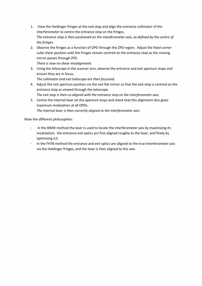
Figure 3. Fringe viewer mounted in interferometer compartment. The upward folding mirror on the baseplate deflects the beam vertically so that the exit stop image appears at the eyepiece - only the eyepiece holder is shown.

e) Move the scanner mirror to a position 200-300 mm from Zero Path Difference (ZPD). f) The fringes should be immediately obvious if the scanner is not moving. Their centre defines

the interferometer axis. You might have to wait for everything to become stable, avoid air movements and/or immobilise the scanner so that it doesn't vibrate to see them. The aim is to centre the entrance stop on the fringe pattern. Adjust M2 with small movements as required to centre the stop on the fringes. Warning! As with any 3-point mirror adjustment system, do not adjust the central adjusting screw of the mirror, as this will change the collimator focus (OAP-entrance stop distance). Adjust only the diagonally-opposite X and Y screws.

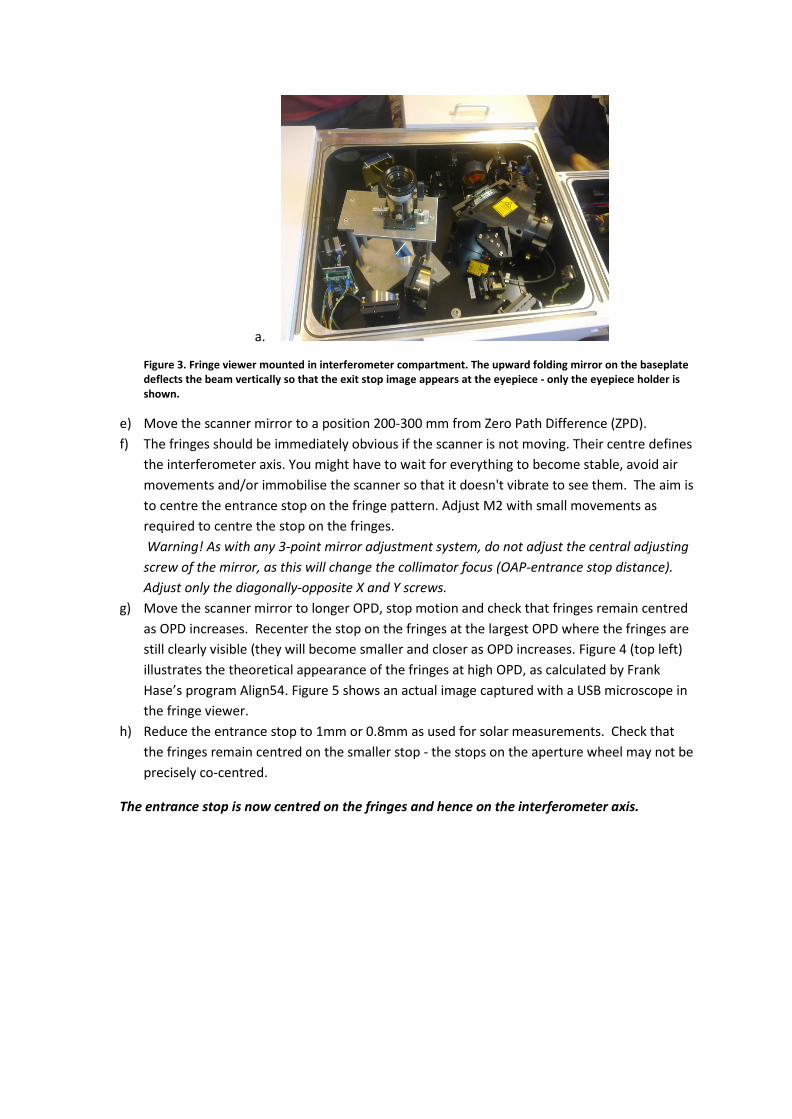
g) Move the scanner mirror to longer OPD, stop motion and check that fringes remain centred as OPD increases. Recenter the stop on the fringes at the largest OPD where the fringes are still clearly visible (they will become smaller and closer as OPD increases. Figure 4 (top left) illustrates the theoretical appearance of the fringes at high OPD, as calculated by Frank Hase’s program Align54. Figure 5 shows an actual image captured with a USB microscope in the fringe viewer.

h) Reduce the entrance stop to 1mm or 0.8mm as used for solar measurements. Check that the fringes remain centred on the smaller stop - the stops on the aperture wheel may not be precisely co-centred.

The entrance stop is now centred on the fringes and hence on the interferometer axis.

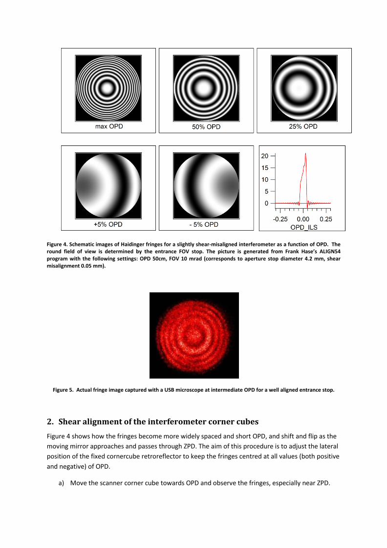
Figure 4. Schematic images of Haidinger fringes for a slightly shear-misaligned interferometer as a function of OPD. The round field of view is determined by the entrance FOV stop. The picture is generated from Frank Hase’s ALIGN54 program with the following settings: OPD 50cm, FOV 10 mrad (corresponds to aperture stop diameter 4.2 mm, shear misalignment 0.05 mm).

Figure 5. Actual fringe image captured with a USB microscope at intermediate OPD for a well aligned entrance stop.

2. Shear alignment of the interferometer corner cubes Figure 4 shows how the fringes become more widely spaced and short OPD, and shift and flip as the moving mirror approaches and passes through ZPD. The aim of this procedure is to adjust the lateral position of the fixed cornercube retroreflector to keep the fringes centred at all values (both positive and negative) of OPD.

a) Move the scanner corner cube towards OPD and observe the fringes, especially near ZPD.

b) If the fringes move off centre and flip on either side of ZPD (for example as in the +5% and -5% OPD images in Figure 4 and the actual images in the Appendix), loosen the locking screws on the fixed cornercube mount (8mm Allen key). The mirror holder can then be moved laterally against springs and adjusted by the two perpendicular adjusting screws.

c) By trial and error (small adjustments!!) adjust the X and Y position of the retroreflector and observe the fringes on either side of ZPD until the fringes are centred and there is no observable flip.

d) Lock the retroreflector screws and recheck.

If your interferometer is badly aligned at the start, you may need to iterate the entrance stop and shear alignments 1 and 2 to get a consistent result.

The retroreflector shear alignment is now correctly adjusted.

3. Align the exit stop to the interferometer axis

Figure 6. Telescope mounted in the scanner compartment. Inset: image of the entrance stop through the telescope with internal laser centred on the stop (step 4).

a) Remove the fringe viewer and block the external laser. b) Prefocus the telescope to infinity by focussing on a distant object and lock the focus.

c) Mount the telescope in the scanner arm in front of the moving cornercube. The telescope should be centred on the IR beam, aligned parallel to the axis and viewing towards the beamsplitter. See Figure 6.

d) Block the exit path and/or illuminate the back side of the entrance stop (LED flashlight, mobile phone light, LED-fibre illuminator are all suitable) and view the stop in the entrance aperture wheel through the telescope. (Remember this stop is already aligned on the interferometer axis in step 1.) Check the focus – this is only a coarse check because the refracting telescope is focussed at infinity for visible wavelengths and may not be precisiely focussed at infinity at the IR wavelengths. We assume here that the focus of the collimator has been correctly set at the factory.

e) Unblock the exit path, illuminate the front of the exit stop aperture wheel and view both entrance and exit apertures at the same time.

f) Adjust the last exit branch flat mirror (M7) to centre the image of the exit stop on the entrance stop. Note that Bruker by default set the exit stop one size larger than the entrance, so the entrance is the limiting stop for field of view.

The exit stop is now aligned to the interferometer axis.

The interferometer is now aligned for IR radiation entering and exiting through the entrance and exit stops. Do not further adjust any optical element M1-M7 between the two stops!

4. Align the internal laser to the interferometer axis. The internal metrology laser should also be aligned parallel to the interferometer axis, and should show the minimum loss of modulation efficiency as OPD increases. The laser does not reflect from any of the IR mirrors (except the interferometer corner cubes M3 and M4), so its alignment is independent of the IR alignment. To adjust the laser optically using the telescope:

a) The laser enters the interferometer compartment vertically from below through a small window and is turned horizontally by a small prism (M8). Check that the laser passes near the centre of the window and the folding prism. Check that the laser hits near the edge of the corner cube of the scanner arm and returns from the opposite edge. The laser should then hit both the small laser mirrors (M9, M10) in each branch; these parabolic mirrors direct the laser onto the two laser detectors.

b) Lower the laser detector mirrors (push down while releasing the pin on the side) so the laser passes above the mirrors to the entrance and exit stops. With the minimum stop size of 0.5 mm, the laser should pass through both stops – if not, adjust using the input folding prism (fine adjustment). The laser should now be withing one stop radius of the correct axis.

c) With vellum or other semitransparent material behind the stops, observe the stops through the telescope – the laser spot should be tightly focussed and centred on the stop (see insert of Figure 6.)

d) Remove the telescope and check the laser modulation as a function of OPD. It is best to use an oscilloscope to view the laser A and B signals - see the Bruker IFS125 manual for details, the signals are available on the PCB near the beamsplitter (Figure 1) and on terminal pins on the external electronics module. The laser signals are the interferogram of the laser - cosine

waves as a function of OPD, and should not lose more than a few percent amplitude between ZPD and OPD. If an oscilloscope is not available, the scanner diagnostic can tell you the laser signal amplitude near ZPD and max OPD. - View the laser A and B amplitudes in the Diagnostics/Scanner page from either OPUS or the webpages. Check the Auto Reload button to get continuous updates of the laser voltages. - Alternately put the scanner in short front adjust and short back adjust modes and observe the laser amplitudes at short and long OPD.

e) You may need to iterate b) – d) to get optimum alignment. f) Frank Hase makes the following additional comment to this step: I prefer to align the laser by

checking explicietly the interference fringes in the laser beam (put a paper just in front of lasa diode) when the scanner is at OPDmax. The condition of passing through the smallest aperture is just a final consistency check - it should be fulfilled automatically if all went right. The observation of the laser spot at OPDmax is also useful for optimal adjustment of the laser beam divergence (I slightly misalign the laser to see two separated spots, then I adjust the beam expander to reach the same diameter in both spots, then I realign for nice circular fringes on the paper.)

The internal laser is now aligned the interferometer axis.

5. Run a cell spectrum and characterise the ILS The interferometer is now in principle aligned. Run a low pressure cell spectrum using the standard TCCON HCl cell and analyse the spectrum with Linefit to characterise the ILS. Figure 7 shows an example from Darwin after following the described alignment procedure.

Note: In using the HCl cell spectra and Linefit to retrieve the ILS, it is important to know the true linewidths of the HCl lines in the spectrum. An error in assumed linewidth aliases into an error in retrieved modulation efficiency (ME), since both affect the final apparent linewidths in the spectrum. For example, assuming a wider true linewidth in Linefit will result in a narrower retrieved ILS (higher ME). The true linewidths are adjusted in Linefit by adjusting the total and partial pressures specified for the HCl. In 2013 Frank Hase determined the effective pressures for each TCCON HCl cell required in Linefit to define the true linewidths see Hase et al., 2013). It is important to use this effective pressure Peff for the total (Ptot) and partial (Ppart+) pressures of HCl in the Linefit retrieval. Note that this effective pressure is in general not the same as the nominal fill pressure of the cell, and may not be self-consistent with the retrieved column amount of HCl (because the pressure measurement at fill-time may have been inaccurate, and because the Hitran linewidths may not be accurate).

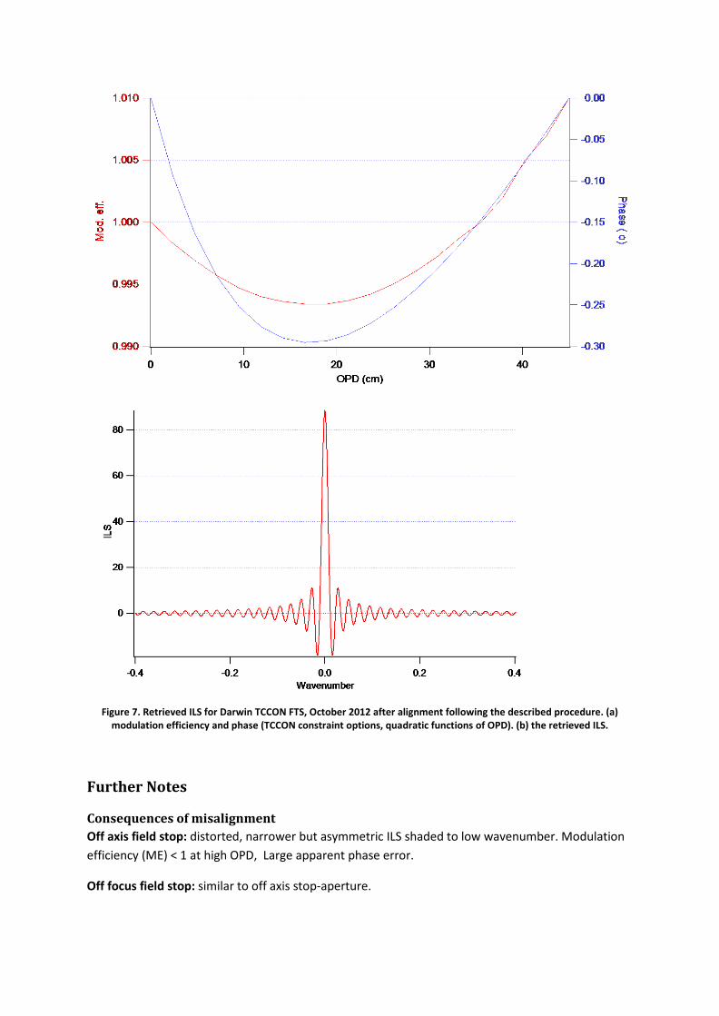
Figure 7. Retrieved ILS for Darwin TCCON FTS, October 2012 after alignment following the described procedure. (a) modulation efficiency and phase (TCCON constraint options, quadratic functions of OPD). (b) the retrieved ILS.

Further Notes

Consequences of misalignment Off axis field stop: distorted, narrower but asymmetric ILS shaded to low wavenumber. Modulation efficiency (ME) < 1 at high OPD, Large apparent phase error.

Off focus field stop: similar to off axis stop-aperture.

Shear misalignment: loss of modulation near ZPD (see Figure 4) gives apparent overmodulation at high OPD (greater than the modulation at ZPD). Leads to narrower ILS than theoretical and ME > 1 in linefit.

Laser off axis alignment: does not affect ILS, but compresses wavenumber scale to lower frequencies. Note: Bruker may artificially adjust the effective laser wavenumber upwards to compensate during final testing. This is false, cancelling one error with another. We recommend the laser wavenumber be set to its correct value, LWN=15798.013 cm-1 (Direct command entry: LWN=15798.013). The observed wavenumber shifts of lines relative to Hitran or other standards are then a useful diagnostic for laser alignment.

Source, sample and detector compartment alignment. The ILS is not dependent on the optics outside the interferometer, assuming the beam is uniform, not masked or wildly off axis, and the detector is uniformly illuminated. To align the source, sample compartment and detector optics, use a visible beam and transparent beamsplitter (eg. CaF2 or quartz) to trace the beam through the system. Start at the source, and centre the beam by eye on each optical element in the path in turn, finishing at the detector. Align the final detector OAP to maximise the signal on the detector (avoiding saturation!)

More on telescope, camera, USB microscope etc.

Viewing the fringes.

The fringes are viewed at the plane of the exit stop by folding the beam upwards into a viewer. The simplest viewer is a telescope eyepiece, and use your eyes. Be careful of laser light. With this solution you can see but not record the fringes.

A DSLR camera connected through a telescope adapter T-ring adapter can be used, see http://en.wikipedia.org/wiki/T-mount for more info. The camera (without lens) replaces the eyepiece with the camera sensor at the focus. The image of the stop and fringes is not magnified, but the camera CCD array has sufficient resolution. Live screen view allows both viewing an expanded image, and recording an image or movie.

Alternatively, a USB microscope (Figure 8) can be used in place of the DSLR camera to view and record images of the fringes. We found this to be a lot simpler and cheaper than the DSLR camera option. USB microscopes are readily available from consumer electronics stores such as Jaycar, see also for example http://www.veho-uk.com/main/shop.aspx?category=usbmicroscope or Amazon.com; cost <$100. The USB microscope results in a large image of the fringes displayed on the computer screen, such as that in Figure 5. See Appendix A for examples of the fringes at different mirror positions as seen via the microscope. The USB microscope may need an adapter ring or tube to attach to the telescope eyepiece holders in the fringe viewer and the telescope (see below).

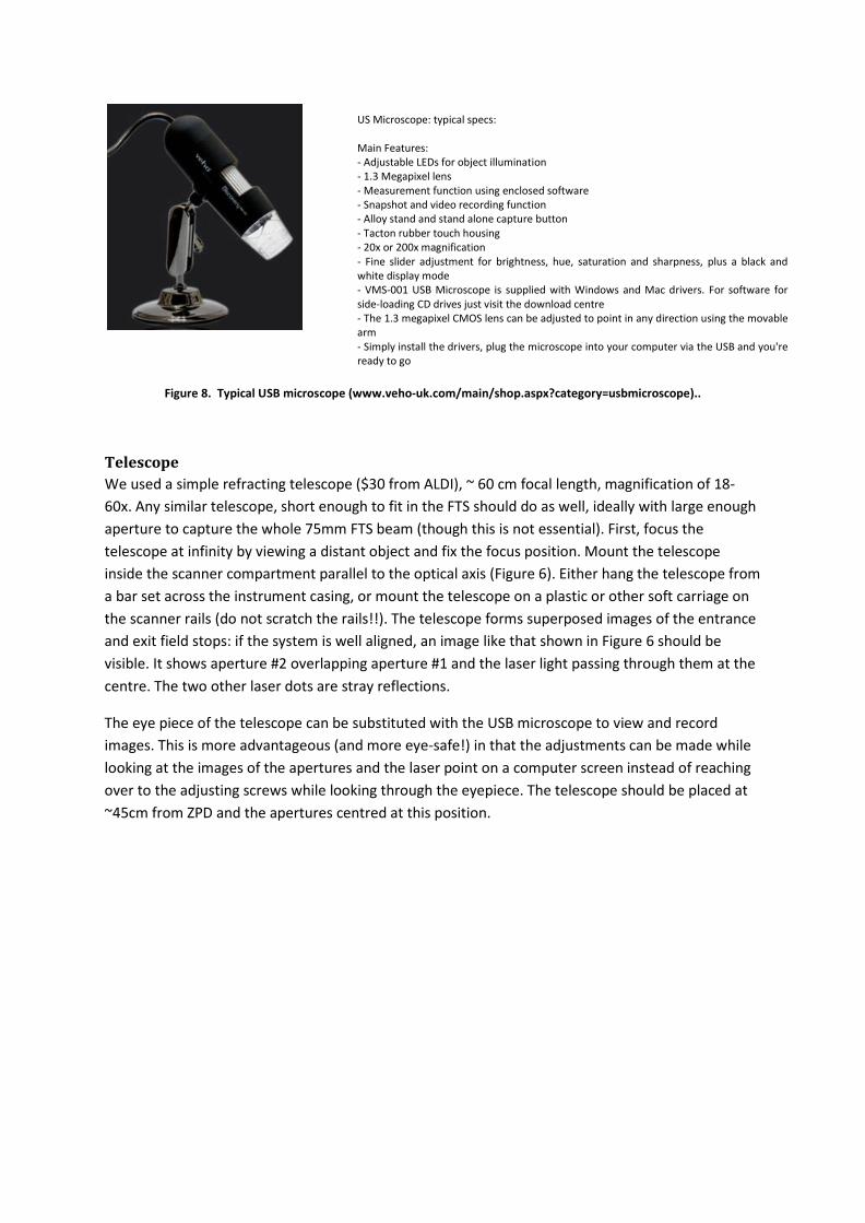
Figure 8. Typical USB microscope (www.veho-uk.com/main/shop.aspx?category=usbmicroscope)..

Telescope We used a simple refracting telescope ($30 from ALDI), ~ 60 cm focal length, magnification of 18-60x. Any similar telescope, short enough to fit in the FTS should do as well, ideally with large enough aperture to capture the whole 75mm FTS beam (though this is not essential). First, focus the telescope at infinity by viewing a distant object and fix the focus position. Mount the telescope inside the scanner compartment parallel to the optical axis (Figure 6). Either hang the telescope from a bar set across the instrument casing, or mount the telescope on a plastic or other soft carriage on the scanner rails (do not scratch the rails!!). The telescope forms superposed images of the entrance and exit field stops: if the system is well aligned, an image like that shown in Figure 6 should be visible. It shows aperture #2 overlapping aperture #1 and the laser light passing through them at the centre. The two other laser dots are stray reflections.

The eye piece of the telescope can be substituted with the USB microscope to view and record images. This is more advantageous (and more eye-safe!) in that the adjustments can be made while looking at the images of the apertures and the laser point on a computer screen instead of reaching over to the adjusting screws while looking through the eyepiece. The telescope should be placed at ~45cm from ZPD and the apertures centred at this position.

US Microscope: typical specs: Main Features: - Adjustable LEDs for object illumination - 1.3 Megapixel lens - Measurement function using enclosed software - Snapshot and video recording function - Alloy stand and stand alone capture button - Tacton rubber touch housing - 20x or 200x magnification - Fine slider adjustment for brightness, hue, saturation and sharpness, plus a black and white display mode - VMS-001 USB Microscope is supplied with Windows and Mac drivers. For software for side-loading CD drives just visit the download centre - The 1.3 megapixel CMOS lens can be adjusted to point in any direction using the movable arm - Simply install the drivers, plug the microscope into your computer via the USB and you're ready to go

Figure 9. Additional equipment

Results

Laser Voltages The table below outlines the laser voltages before and after the alignment of the Wollongong IFS 125 spectrometer. Note that the voltages did not change much, this is because the FTS was already well aligned to begin with. The differences before and after the alignment become obvious once a LINEFIT analysis is performed (next chapter, Fig. 5).

Before alignment

(27 Sep '12)

After alignment

(2 Oct '12)

Volts (pk-

ZPD MaxOPD ZPD MaxOPD ZPD MaxOPD

A. Telescope and improvised holder B. Rail to hold the telescope above the scanner arm of the IFS-125 C. USB microscope D. Periscope eyepiece E. Periscope mount and flat reflecting mirror F. HeNe laser with beam expander and mount G. HeNe Laser power supply H. Vellum and paper for blocking laser beams

pk) KBr

Laser A

15 13.8 15.2 12.8 10.2 8.4

Laser B

10 9 10 8.4 5.4 4.4

Linefit Analysis Analysis using LINEFIT Ver. 12 (Hase et al., 1999) show a near perfect (100.7%, and most recently at 100.%) modulation efficiency after the alignment procedures described above, see Fig. 5 below.

Figure 9. Modulation efficiency is at 100.% after alignment using the periscope (fringes) and the telescope methods as discussed above. The figure also shows measurements from different cells.

Appendix: Images of the Fringes Taken Via USB Microscope

Indicators of shear misalignment: the fringes shift as you move closer to and past the ZPD (below).

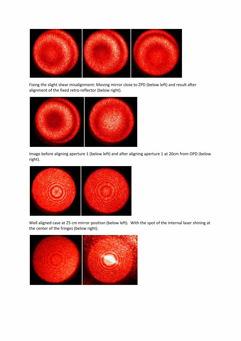
Fixing the slight shear misalignment: Moving mirror close to ZPD (below left) and result after alignment of the fixed retro-reflector (below right).

Image before aligning aperture 1 (below left) and after aligning aperture 1 at 20cm from OPD (below right).

Well aligned case at 25 cm mirror position (below left). With the spot of the internal laser shining at the center of the fringes (below right).

6. References: F. Hase, T.Blumenstock and C. Paton-Walsh, Analysis of instrumental line shape of high-resolution FTIR-spectrometers using gas cell measurements and a new retrieval software, Applied Optics, 38, 3417 - 3422 (1999).

F. Hase et al., Calibration of sealed HCl cells used for TCCON instrumental lineshape monitoring, Atmos. Meas. Techn. (Discussions), 6, 7185-7215 (2013).

Kauppinen, J. and P. Saarinen (1992). "Line shape distortions in misaligned cube corner interferometers." Applied Optics 31(1): 69-74.

Saarinen, P. and J. Kaupinnen (1992). "Spectral line-shape distortions in Michelson interferometers due to off-focus radiation sources." Applied Optics 31(13): 2353-2359.

M. V. R. K. MURTY, "Some More Aspects of the Michelson Interferometer with Cube Corners," J. Opt. Soc. Am. 50, 7-9 (1960) http://www.opticsinfobase.org/abstract.cfm?URI=josa-50-1-7

EDSON R. PECK, "Theory of the Corner-Cube Interferometer," J. Opt. Soc. Am. 38, 1015-1015 (1948) http://www.opticsinfobase.org/josa/abstract.cfm?URI=josa-38-12-1015

EDSON R. PECK, "A New Principle in Interferometer Design," J. Opt. Soc. Am. 38, 66-66 (1948) http://www.opticsinfobase.org/josa/abstract.cfm?URI=josa-38-1-66

F. Hase, T.Blumenstock, Alignment procedure for Bruker IFS 120 spectrometers, Internal Document, 01 Sep 2000.

J. Robinson, Bruker_125_align.pdf and various other alignment notes on the wiki.