IFE Paper - Princeton University

International Friends and Enemies∗

Benny Kleinman†Princeton University

Ernest Liu‡Princeton University

Stephen J. Redding§Princeton University, NBER and CEPR

September 15, 2021

Abstract

To what extent do nations’ economic interests in�uence their political behavior? We pro-vide new evidence on this question using bilateral network measures of exposure to foreigneconomic growth and a range of measures of bilateral political behavior, including UnitedNations voting, strategic rivalries and formal alliances. Using exogenous variation from thenatural experiments of China’s emergence into the global economy and reductions in the costof air travel over time, we show that as a country becomes more economically dependent ona trade partner, it realigns politically towards that trade partner.

Keywords: international relations, trade, productivity growth, welfareJEL Classi�cation: F14, F15, F50

∗We are grateful to Princeton University for research support. We would like to thank Keith Head, Xavier Jaravel,Nathan Lane, Thierry Mayer, Tommaso Porzio, Nancy Qian, Kadee Russ, Johannes Stroebel and conference andseminar participants at China Economics Summer Institute, Federal Reserve Bank of Atlanta/Emory University,Geneva Online Trade and Development Workshop, Harvard-MIT, Hong Kong University of Science and Technology,Nottingham University, National Bureau of Economic Research (NBER), National University of Singapore, PekingUniversity, Penn State University, Princeton University, Queen Mary University of London, the RIDGE Conferencein Trade and Development, the STEG Annual Conference 2021, and the World Bank for helpful comments andsuggestions. We are grateful to Xavier Jaravel for sharing the strategic rivalry data. We also would like to thankGordon Ji, Ian Sapollnik and Maximilian Schwarz for excellent research assistance. The usual disclaimer applies.

†Dept. Economics, JRR Building, Princeton, NJ 08544. Email: [email protected].‡Dept. Economics, JRR Building, Princeton, NJ 08544. Email: [email protected].§Dept. Economics and SPIA, JRR Building, Princeton, NJ 08544. Email: [email protected].

1 Introduction

“Throughout history, anxiety about decline and shifting balances of power has beenaccompanied by tension and miscalculation ... Traditionally the test of a great powerwas its strength in war. Today, however, the de�nition of power is losing its emphasison military force ... The factors of technology ... and economic growth are becomingmore signi�cant in international power.” (Nye 1990, pp. 153-4)

To what extent do nations’ economic interests in�uence their political behavior? We provide newevidence on this question using network measures of the sensitivity of welfare in one countryto productivity growth in another country. We propose a bilateral friends-and-enemies matrixrepresentation of the �rst-order general equilibrium e�ect of productivity growth in one countryon welfare in another: One country is a friend [enemy] for income or welfare in another countryif its productivity growth raises [reduces] the income or welfare of the other country. UsingChina’s emergence into the global economy as a natural experiment, we show that as countriesbecome more economically dependent on China relative to the United States over time, theyrealign politically away from the United States and towards China, with this pattern particularlystrong for South-East Asian and resource-rich African countries. More broadly, using exogenousvariation in bilateral trade costs within exporter-importer pairs over time from the declining costof air travel, we show that as a country’s welfare becomes more exposed to productivity growthin another nation, it realigns politically towards that nation, along a range of measures includingUnited Nations voting, strategic rivalries and formal alliances.1

Analyzing the relationship between political behavior and economic interests raises severalchallenges. First, there is the problem of measuring the sensitivity of one country’s welfare toproductivity growth in another country. Some studies use bilateral trade. However, one coun-try’s economic exposure to another does not only depend on bilateral trade frictions, but alsoon trade frictions with other nations. Even taking this multilateral resistance into account yieldsan incomplete picture, because productivity growth in trade partners typically has other generalequilibrium e�ects through the terms of trade. Another approach is to undertake counterfactu-als for productivity shocks within a non-linear general equilibrium trade model. However, thisapproach also faces challenges, because it requires a measure of productivity growth to evalu-ate these counterfactuals. Although actual productivity growth can be measured using observeddata, political behavior does not only depend on the actual shocks that occurred, but also on thecounterfactual shocks that could have occurred. For example, a country’s political behavior can

1Recent work emphasizing links between economics and politics includes research on trade and war (Martin et al.2008), institutions and development (Acemoglu et al. 2001), foreign aid and development (Kuziemko andWerker 2006;Nunn and Qian 2014); and economic networks and con�ict (König et al. 2017).

1

depend on expected events or policies in its trade partners, but such counterfactual shocks cantake many possible values and are typically unobserved.

Our network measures address these challenges. First, they correspond to the elasticities ofcountry welfare with respect to foreign productivity growth in the class of international trademodels with a constant trade elasticity. Hence, they correspond exactly to the theoretically-consistent measure of the sensitivity of country welfare with respect to productivity growth inthis in�uential class of models. Second, they can be computed directly from observed trade dataalone, which avoids the requirement of having to measure counterfactual shocks that in�uencedcountry behavior but which did not in fact occur. Third, since our measures are derived fromthe general equilibrium conditions of this class of models, they capture not only multilateralresistance but all �rst-order general equilibrium e�ects. Finally, we show that our sensitivitymeasures are not only exact for small shocks but provide a good approximation to the full non-linear model solution for empirically-realistic shocks, such as cumulative changes in productivityover our sample period of more than forty years.

We obtain our friends-and-enemies measures of bilateral exposure from a matrix represen-tation of the �rst-order comparative statics in constant elasticity trade models. An advantage ofthis matrix representation of the entire bilateral network of country income and welfare exposureis that we are able to use techniques from the networks literature to characterize the role of coun-tries’ positions within the network in in�uencing the e�ects of productivity shocks. We evaluatethe extent to which each country’s productivity growth a�ects others (its “authority score” fromgraph theory) and the extent to which each country is a�ected by others’ productivity growth (its“hub score” from graph theory). We thus provide new data on countries’ roles in the global econ-omy, both in terms of our measures of income and welfare exposure, and the network statisticsderived from them. Our use of the terms “friends” and “enemies” echoes its use in neoclassicaltrade theory for the general equilibrium relationships between factor and goods prices, or goodsoutputs and factor endowments.

We combine our economic exposure measures with a range of di�erent measures of countries’political alignment. First, we use three di�erent measures of the bilateral similarity of countries’voting patterns in the United Nations General Assembly (UNGA). Second, we use measures ofcountries’ “ideal points” or preferences relative to the US-led liberal order, based on the UNGAvoting data. Third, we use measures of strategic rivalries, based on the perceptions of contempo-rary political decisions, as to whether countries regard one another as actual or latent threats. Wefurther disaggregate these strategic rivalries into those that are positional, spatial and ideological.Finally, we use measures of formal alliances between countries, including mutual defense pacts,neutrality and non-aggression treaties and ententes.

Another challenge in examining the relationship between political behavior and economic

2

interests is that causality can run in both directions, or both variables can be in�uenced by omit-ted third factors. We address this challenge in two ways. First, we use the natural experimentof China’s liberalization in 1978. Following China’s market-orientated reforms, we show thatother countries realign politically towards China and away from the United States. We showthat this realignment is stronger for Africa and Asia/Oceania, and weaker for Europe and Northand South America. Over the same period, we observe an increase in other countries’ welfareexposure to China relative to the United States. We �nd that this change in relative welfare ex-posure is stronger for Africa and Asia/Oceania, and weaker for Europe and North and SouthAmerica. Therefore, there is a close relationship between the observed political realignment andthe change in relative welfare exposure following China’s emergence into the global economy,consistent with economic interests shaping political behavior. As further evidence in support ofthis relationship, we �nd that countries with initially higher levels of exposure to productivitygrowth in any nation, according to their initial network hub score, experience larger changes inpolitical realignment towards China and away from the United States.

Second, we make use of the large-scale reduction in the cost of air travel that occurred overour sample period following Feyrer (2019). The key idea is that the position of landmasses aroundthe globe generates large di�erences between bilateral distances by sea and air, such that somebilateral pairs bene�t more from the reduction in the cost of air travel than others. By exploitingvariation in trade costs over time within exporter-importer pairs, we control for a host of time-invariant factors that are speci�c to individual pairs of countries (e.g. geographical location, in-stitutions, legal origin, common language etc.). We also include exporter-year and importer-year�xed e�ects, which control for the sign and absolute magnitude of actual or expected exporterproductivity growth, as well as policy changes that are common to all trade partners and macroshocks. Using these di�erential changes in relative trade costs from reductions in the cost of airtravel within exporter-importer pairs, we �nd that increases in bilateral welfare exposure raisebilateral political alignment. We show that these results are robust across a range of econometricspeci�cations (including panel and long-di�erences regressions) and measures of bilateral polit-ical alignment (including UN voting, strategic rivalries and formal alliances). Therefore, these�ndings provide further support for the view that as a country becomes more economically de-pendent on its trade partner, it realigns politically towards that trade partner.

We �rst introduce our friend-enemy exposure measures for the in�uential class of single-sector models with a constant trade elasticity. We next show that this same representation holdsacross a wide range of speci�cations, including a state of the art quantitative trade model withmultiple sectors and input-output linkages. We use this quantitative speci�cation for our mainempirical results and report a number of further validation exercises. First, we show that ourexposure measures are not well proxied by simpler measures of economic relationships between

3

countries, such as bilateral trade �ows. Second, we provide evidence that our model-based expo-sure measures have predictive power for separate data not used in their estimation. We show thatour exposure measures both predict country selection into preferential trade agreements (PTAs)and detect increases in economic interdependence following the formation of these PTAs.

Our research contributes to several strands of existing work. First, our paper is related toresearch on international political economy. One strand of this research has measured countries’bilateral political alignment using data on the similarity of their voting patterns in the UnitedNations General Assembly (UNGA), including Scott (1955), Cohen (1960), Signorino and Ritter(1999), Häge (2011) and Dicaprio and Sokolova (2018). Much of this literature focuses on thebilateral similarity of these voting patterns. In contrast, Bailey et al. (2017) uses information on theissues voted on to estimate countries’ “ideal points,” which correspond to their positions vis-a-visthe US-led liberal order.2 Another line of this research has measured countries’ bilateral politicalalignment using data on strategic rivalries, based on the perceptions of contemporary politicaldecision markers, including Thompson (2001), Colaresi et al. (2010) and Aghion et al. (2018).Another branch of work has used data on formal alliances between countries, including Eisenseeand Strömberg (2007), Gartzke (2007) and de Mesquita and Siverson (1995). A further vein of thisresearch measures bilateral political attitudes using survey data and other information, includingAlesina and Spolaore (2003), Guiso et al. (2009), Head et al. (2010), Head and Mayer (2013) andBao et al. (2019). Our key contribution relative to this literature is to examine the relationshipbetween these measures of bilateral political alignment and our new measures of the extent towhich countries are economic friends and enemies.3

Second, our research connects with the empirical literature on war and trade. One strandof this work looks at the causal impact of war on trade, including Blomberg and Hess (2006)and Glick and Taylor (2010). Another line of this work looks at the opposite causal relationshipof trade on the probability of con�ict, including Polachek (1980), Mans�eld (1995) and Barbieri(2002). Combining these two strands, Martin et al. (2008) provide theory and evidence that glob-alization decreases the likelihood of global con�ict, but increases the chance of bilateral con�ict,because globalization increases countries’ multilateral dependence on one another as a whole,but decreases a country’s bilateral dependence on any one trade partner. Although the use ofmilitary force is the ultimate expression of political power, it is relatively rare. Furthermore, the

2Using UN and US data, Kuziemko and Werker (2006) shows that aid to a country increases when it rotates ontothe Security Council. Using US aid data, Nunn and Qian (2014) shows that an increase in food aid increases theincidence and duration of civil con�icts. Using trade data, Meyersson et al. (2008) examines the impact of China’sdemand for natural resources on human rights in Sub-Saharan Africa.

3Several authors have drawn parallels between the current China-US tensions and earlier episodes of changingrelative economic size, such as Japan and the United States in the 1980s, Britain and Germany at the turn of the 20thcentury, or Athens and Sparta in Ancient Greece. See Brunnermeier et al. (2018) and “China-US rivalry and threatsto globalization recall ominous past, ” Martin Wolf, Financial Times, 26th May, 2020.

4

international relations literature emphasizes softer forms of political power, including interna-tional agreements, supra-national institutions, and back-room diplomacy (see for example Nye1990). We provide new theory and evidence on the extent to which these softer forms of politicalpower are in�uenced by economic interests.

Third, we build on the empirical literature that has developed instrumental variables for bi-lateral international trade, including Frankel and Romer (1999), Rodriguez and Rodrik (2001) andFeyrer (2019). Fourth, we also build on research on quantitative models and su�cient statisticsin trade, including Armington (1969), Jones and Scheinkman (1977), Wilson (1980), Eaton andKortum (2002), Anderson and van Wincoop (2003), Arkolakis et al. (2012), Costinot et al. (2012),Caliendo and Parro (2015), Adão et al. (2019), Baqaee and Farhi (2019), Huo et al. (2019), Caliendoet al. (2019) and Allen et al. (2020).4 Our key departure from this literature is in the manipulationof the system of linearized market clearing conditions into two matrices of bilateral income andwelfare exposure. This procedure generates two sets of bilateral statistics on the global trade net-work that can be taken as inputs for further empirical analysis. These matrices capture the fullnetwork of bilateral income and welfare elasticities, which allows us to make use of tools fromthe network analysis literature, and these measures can be integrated into other dyadic datasets.We show that our representation holds across a wide range of trade models, including speci�ca-tions with multiple sectors and input-output linkages. We use this representation to provide ananalytical characterization of the quality of the �rst-order approximation to the full non-linearmodel solution in terms of these observed matrices. In our empirical application, we use ournetwork measures to provide new evidence on the substantive question of the extent to whichcountries’ economic interests shape their political behavior.

The remainder of the paper is structured as follows. Section 2 derives our economic friendsand enemies measures. Section 3 introduces our data. Section 4 reports our main empirical re-sults on political and economic friends. Section 5 reports further speci�cation checks. Section 6concludes. A separate online appendix contains the derivations of the results in the paper and anumber of further extensions.

2 Economic Friends and Enemies

In this section, we propose a bilateral friends-and-enemies matrix representation of the �rst-order comparative statics of productivity growth in one country on the income and welfare inanother country in constant elasticity trade models. We �rst develop our exposure measuresfor an in�uential class of single-sector models. We next derive our measures for a state of the

4The earlier theoretical literature on foreign productivity growth and domestic welfare includes the classic con-tributions of Hicks (1953), Johnson (1955) and Bhagwati (1958).

5

art quantitative trade model with multiple sectors and input-output linkages. For simplicity, wefocus on Armington trade models, in which goods are di�erentiated by origin. In Section C ofthe online appendix, we demonstrate isomorphisms with the entire class of trade models with aconstant trade elasticity.

2.1 Model

Consider a world of many countries indexed by n, i 2 {1, . . . , N}. Each country has an ex-ogenous supply of `n workers, who are each endowed with one unit of labor that is suppliedinelastically. Goods are di�erentiated by country of origin and the representative consumer incountry n is assumed to have constant elasticity of substitution (CES) preferences, such that theindirect utility function (un) takes the following form:

un =wn

hPN

i=1 p�✓

ni

i� 1✓

, ✓ = � � 1, � > 1, (1)

where wn is the wage; pni is the price in country n of the good produced in country i; � > 1 isthe elasticity of substitution and ✓ = � � 1 is the trade elasticity. Using Roy’s Identity, countryn’s share of expenditure on the good produced by country i (sni) is:

sni =p�✓

niPN

m=1 p�✓nm

. (2)

Each country’s good is produced with labor according to a constant returns to scale productiontechnology, with productivity zi in country i. Markets are perfectly competitive. Goods can betraded between countries subject to iceberg trade costs, such that ⌧ni � 1 units of a good mustbe shipped from country i in order for one unit to arrive in country n (where ⌧ni > 1 for n 6= i

and ⌧nn = 1). The cost in country n of consuming one unit of the good produced by country i is:

pni =⌧niwi

zi. (3)

Goods market clearing requires that income in country i equals the expenditure on goods pro-duced by that country:

wi`i =NX

n=1

sniwn`n, (4)

where we begin by assuming for simplicity that is balanced, before later generalizing our ap-proach to allow for trade imbalances. Finally, we choose world GDP as the numeraire:

NX

n=1

wn`n = 1. (5)

Using these components of the model, we are now in a position to de�ne general equilibrium.

6

Equilibrium Given fundamentals, i.e., the set of country-level productivities {zi} and bilateraltrade costs {⌧ni}, the general equilibrium of themodel is the collection of factor prices {wi}, goodsprices {pni}, and expenditure shares {sni}, and welfare {un} that satisfy equations (1)-(5).

Substituting the expenditure share (2) and pricing rule (3) into the market clearing condition(4), we can reduce the general equilibrium of the model to a single system of N equations thatuniquely determines the N wages in each country.

2.2 First-Order Comparative Statics

We next derive familiar �rst-order comparative statics in this class of constant elasticity trademodels,5 before introducing our new friend-enemy representation in the next section. Totallydi�erentiating the expenditure share (2), the pricing rule (3) and the market clearing condition(4), the change in country income per capita satis�es:

d lnwi =NX

n=1

tin

d lnwn + ✓

NX

h=1

snh [ d ln ⌧nh + d lnwh � d ln zh]� [ d ln ⌧ni + d lnwi � d ln zi]

!!, (6)

where we have held country labor endowments constant ( d ln `i = 0) and the share of valueadded that country i derives from each market n is de�ned as:

tin ⌘ sniwn`nwi`i

.

Totally di�erentiating the indirect utility function (1), the change in country welfare equals thechange in income per capita minus the expenditure share weighted average of price changes:

d ln un = d lnwn �NX

i=1

sni [ d ln ⌧ni + d lnwi � d ln zi] . (7)

2.3 Friends-and-Enemies Representation

The friend-enemy representation of bilateral economic exposure stacks the �rst-order compara-tive statics into a matrix that captures the e�ect on each country (rows) of shocks in any othercountry (columns), where one country is a friend [enemy] for income or welfare in another coun-try if its productivity growth raises [reduces] the income or welfare of the other country. Thefriend-enemymatrix therefore represents the entire bilateral network of country income andwel-fare exposure to foreign shocks and enables us to use techniques from the networks literature tocharacterize the role of countries’ positions within the global economic network.

5See, for example, Jones and Scheinkman (1977), Wilson (1980), Arkolakis et al. (2012), Adão et al. (2019), Baqaeeand Farhi (2019), and Huo et al. (2019).

7

We use boldface, lowercase letters for vectors, and boldface, uppercase letters for matrices.We use the corresponding non-bold, lowercase letters for elements of vectors and matrices. Weuse I to denote the N ⇥N identity matrix.

Expenditure Share and Income Share Matrices Let S ⌘ [sni] be the N ⇥ N matrix withthe ni-th element equal to importer n’s expenditure share on exporter i. Let T ⌘ [tin] be theN ⇥N matrix with the in-th element equal to the fraction of income that exporter i derives fromselling to importer n. We refer to S as the expenditure share matrix and to T as the income sharematrix. Intuitively, sni captures the importance of i as a supplier to country n, and tin capturesthe importance of n as a buyer for country i. Note the order of subscripts: in matrix S, rowsare buyers and columns are suppliers, whereas in matrix T, rows are suppliers and columns arebuyers. Both matrices have rows that sum to one.6

Let q ⌘ [wi`n] be theN ⇥ 1 vector with the i-th element equal to country i’s income relativeto world GDP. We refer to q simply as the income vector.

The q vector and the S andTmatrices are all equilibrium objects that can be obtained directlyfrom observed trade data. Under trade balance, q0 is the dominant left-eigenvector of both S andT , with corresponding eigenvalue of one.

Friends-and-Enemies for Income Using the matrix notation, we can stack the comparativestatics for income in equation (6) as:

d lnw| {z }income e�ect

= T d lnw| {z }market-size e�ect

+ ✓ ·M⇥ ( d lnw � d ln z)| {z }cross-substitution e�ect

, (8)

where we denote M ⌘ TS � I . The income comparative statics in equation (8) have an in-tuitive interpretation. The �rst term on the right-hand side captures a market-size e�ect. If theproductivity shocks raise income in another country n, this raises income in country i throughincreased expenditure on its goods. The magnitude of this e�ect depends on the share of incomethat country i derives from country n (as captured by the matrix T ).

The second term on the right-hand side captures a cross-substitution e�ect, where the in-thelement of the cross-substitution matrix (M ⌘ TS � I) is given by min ⌘

PN

h=1 tihshn � 1n=i.For i 6= n, the sum

PN

h=1 tihshn captures the overall competitive exposure of country i to countryn, through each of their common markets h, weighted by the importance of market h for country

6For theoretical completeness, we maintain two assumptions on S, which are satis�ed empirically in all years ofour data: for any i, n, there exists k 2 Z+ such that

⇥Sk⇤in

> 0; (ii) for all i, sii > 0. The �rst assumption states thatall countries are connected through trade, directly or indirectly. Theoretically, this assumption is important becauseshocks propagate in general equilibrium through changes in relative prices, which are only well-de�ned if countriesare connected (potentially indirectly) to each other through trade. The second assumption states that every countryconsumes a positive amount of domestic goods.

8

i’s income (tih). As the competitiveness of country n increases, as measured by a decline in itswage relative to its productivity ( d lnwn� d ln zn), consumers in all markets h substitute towardscountry n and away from other countries i 6= n, thereby reducing income in country i and raisingit in country n. With a constant elasticity import demand system, the magnitude of this cross-substitution e�ect in market h depends on the trade elasticity (✓) and the share of expenditure inmarket h on the goods produced by country n (shn): consumers in market h increase expenditureon countryn by (shn � 1) and lower expenditure on country i by shn. Summing across all marketsh, we obtain the overall impact on country i’s income.

Using our matrix representation of the income comparative statics in equation (8), we canimmediately recover the elasticity of each country’s income with respect to a productivity shockin any country from a simple matrix inversion problem.

De�nition 1. The “friends-and-enemies” income exposure matrix is

W ⌘ � ✓

✓ + 1(I�V)�1 M, V ⌘ T+ ✓TS

✓ + 1�Q,

where Q is an N ⇥N matrix with the income row vector q0 stacked N times.

The elements of the matrix W capture countries’ bilateral income exposure to productivityshocks, as shown in Section B of the online appendix:

d lnw = W d ln z, (9)

In particular, the in-th element of this matrix is the elasticity of income in country i (row) withrespect to a small productivity shock in country n (column). We refer to country n as being a“friend” of country i for income when this elasticity is positive and an “enemy” of country i forincome when this elasticity is negative. In general,W is not necessarily symmetric: i could viewn as a friend, while n views i as an enemy.

Our choice of world GDP as the numeraire implies thatP

N

i=1 qi d lnwi = 0 or Q d lnw = 0,where Q is an N ⇥ N matrix with the income row vector q0 stacked N times. The presence ofthe term Q in the de�nition of the matrix V in De�nition 1 re�ects this choice of numeraire.7 Allof our predictions for relative country incomes are invariant to the choice of numeraire.

7Without this term, the matrix⇣I� T+✓TS

✓+1

⌘is not invertible, because the income shares and expenditure shares

sum to one (P

N

n=1 tin = 1 andP

N

n=1 sni = 1), which implies that the rows of T+✓TS✓+1 sum to one and the columns

of⇣I� T+✓TS

✓+1

⌘are not linearly independent. This non-invertibility re�ects the fact that the trade share matrices

T , S and M are homogeneous of degree zero, which implies that income can only be recovered from these tradeshares up to a normalization or choice of units.

9

Since the spectral radius (largest absolute eigenvalue) of the matrix V is less than one, thematrix inversion in De�nition 1 has a power-series or Neumann-series representation:

W = � ✓

✓ + 1(I�V)�1 M = � ✓

✓ + 1

1X

k=0

VkM = � ✓

✓ + 1M

| {z }partial equilibrium

� ✓

✓ + 1

�V +V2 + . . .

�M

| {z }general equilibrium

.

(10)In this representation, the overall �rst-order impact is expressed in terms of a partial equilibriume�ect, which captures the direct impact of the productivity shocks at initial prices, and generalequilibrium e�ects, which capture the endogenous adjustment of prices.

Friends-and-Enemies forWelfare We next stack the comparative statics for welfare in equa-tion (7) in matrix form:

d lnu| {z }welfare e�ect

= d lnw| {z }income e�ect

� S ( d lnw � d ln z)| {z }cost-of-living e�ect

. (11)

Again the welfare comparative statics in equation (11) have an intuitive interpretation. Thechange in welfare depends on the change in income and a cost of living e�ect, which re�ectsthe impact of the productivity shocks on the price index in each country. This cost of livinge�ect depends on the share of expenditure (sni) that each country n allocates to all countries i,as captured in the S matrix.

De�nition 2. The “friends-and-enemies” welfare exposure matrix is

U ⌘ (I� S)W + S.

The elements of the matrix U capture countries’ bilateral welfare exposure to productivityshocks, as follows from equation (11):

d lnu = U d ln z. (12)

In particular, the ni-th element of this matrix is the elasticity of welfare in country n (row) withrespect to a small productivity shock in country i (column). We refer to country i as being a“friend” of country n for welfare when this elasticity is positive and an “enemy” of country n

for welfare when this elasticity is negative. As for income exposure, welfare exposure U is notnecessarily symmetric: i could view n as a friend, while n views i as an enemy. Unlike the incomeexposure, which captures nominal e�ects of productivity shocks and thus depends on the choiceof numeraire, the welfare exposure in De�nition 2 captures real e�ects of productivity shocksand is thus invariant to our choice of numeraire.

10

ExposureNetwork Our friends-and-enemiesmatrix representations of bilateral exposure lendthemselves to the use of techniques from the networks literature to characterize the role of coun-tries’ positions within the network in in�uencing the e�ects of productivity shocks. In particular,we use the authority and hub scores from Kleinberg (1999), which are generalizations of the cen-trality measures used for symmetric networks. These generalizations take into account that thenetwork is asymmetric and hence the direction of relationships matters. The authority scorecaptures the extent to which a country a�ects others, while the hub score captures the extent towhich a country is in�uenced by others.

More formally, the hub and authority scores for welfare exposure can be retrieved as thedominant eigenvector of UU 0 and U 0U , respectively, such that a / U 0Ua and h / UU 0h.Therefore, we can write these hub and authority scores, {hi, ai}Ni=1, as follows:

ai = �NX

n=1

Unihn, hn = µNX

i=1

Uniai, (13)

where � and µ are scaling constants that are equal to the inverse norms of the vectors a ⌘ [ai]

and h ⌘ [hn], respectively. Intuitively, countries with higher authority scores are those whoseproductivity growth has a larger impact on other countries. In contrast, countries with higherhub scores are those more highly exposed to productivity growth in other countries. From thebilateral country-partner network of exposure, we can thus obtain measures for each country ofthe extent to which it in�uences others and the extent to which it is in�uenced by others, forboth income and welfare exposure.

Non-linearities Our exposure measures in equations (9) and (12) are derived from a lineariza-tion that is exact for small shocks. In Section 5 below and in SectionH.2 of the online appendix, weshow that these exposure measures provide a good approximation to the full non-linear modelsolution more generally. First, we derive analytical bounds on the absolute magnitude of thenon-linearities not captured by our exposure measures in terms of the observed trade shares andthe trade elasticity (✓). We implement these analytical bounds empirically and con�rm that thenon-linearities are indeed small compared with the �rst-order e�ect captured by our measures.Second, we directly show that our linearization closely approximates the predictions of the fullnon-linear model solution for the empirical distribution of cumulative productivity growth overour sample period of more than forty years from 1970-2012.

Multiple Sectors and Input-Output Linkages To illustrate our approach as clearly as possi-ble, we have so far focused exposition on the in�uential class of single-sector trade models witha constant trade elasticity. An advantage of our friends-and-enemies representation is that it also

11

holds for constant trade elasticity models with multiple industries, such as Costinot et al. (2012),and state-of-the-art models with cross-sector input-output linkages, such as Caliendo and Parro(2015). In both of these extensions, the income andwelfare exposuresmatricesW andU continueto followDe�nitions 1 and 2, and the economic forces shaping these cross-country exposures havethe exact same interpretation of market size, cross-substitution, and cost-of-living e�ects, respec-tively captured by the income share (T ), cross-substitution (M ), and expenditure share (S) ma-trices. These extensions require richer data on industry-level trade and input-output �ows. Thisadditional information not only modi�es the market size, cross-substitution and cost of livinge�ects, and hence changes income and welfare exposure, but also generates extra, industry-levelpredictions for the impact of foreign shocks.

As shown in detail in Sections D.3-D.6 of the online appendix, the di�erences between theexposure measures in these richer models and the single-sector Armington model lie in the con-struction of these S, T , and M matrices. For the multi-sector model without input-output link-ages, the S and T matrices continue to represent country-to-country expenditure shares andincome shares, and the only adjustment to be made relative to the single-sector model is to thecross-substitution M matrix. In the single sector model, recall that the in-th element of the Mmatrix for i 6= n is given by

PN

h=1 tihshn, which captures the overall competitive exposure ofcountry i to country n, through each of their common markets—countries indexed by h—wherein each market h the exposure is the product between the importance of that market for countryi’s income (tih) and the expenditure share of h’s consumers on the goods produced by countryn (shn). In the multi-sector model, the cross-substitution M matrix accounts for the fact that amarket is no longer a third country but is instead a country-industry. The competitive exposureof country i to country n in a country-industry market hk—for instance, countries i and n maycompete for the textiles (k) in Singapore (h)—is the product between the income that country i

derives from exporting textiles to Singapore and Singapore’s within-sector expenditure share ontextile produced by country n.

For the multi-sector input-output model (Caliendo and Parro 2015), the elements of all threematrices must be adjusted to take into account the network structure of production, using theobserved industry-to-industry �ows in the input-output matrix. For the S and T matrices, thisis largely a matter of accounting. We take into account that the gross value of trade includesnot only the direct value-added created in this exporter and industry but also indirect value-added created in previous stages of production, and we unwind production chains so that Sand T capture expenditure and income shares in terms of value-added. For the M matrix, thisadjustment also takes into account that the e�ect of a foreign productivity shock now di�ersdepending on whether it reduces intermediate input costs or competitors’ output prices, as wellas the fact that now competitive pressure is present at every stage of a production chain. For this

12

multi-sector input-output model, the elements of the S, T and M matrices are now given by:

Sni ⌘NX

h=1

KX

k=1

↵k

nsknh⇤k

hi, Tin ⌘

NX

h=1

KX

k=1

⇧k

ih#k

hn, Min ⌘

NX

h=1

KX

k=1

NX

o=1

⇧k

io

#k

oh+

NX

j=1

⇥kj

oh

!⌥k

hon,

where ⇤k

hicaptures the share of production cost in industry k in country h that is spent on value-

added in country i; ⇧k

ihis the network-adjusted income share that country i derives from selling

to industry k in country h; #k

hnis the share of revenue that industry k in country h derives from

selling to country n;⇥kj

ohcaptures the fraction of revenue in industry k in country o derived from

selling to producers in industry j in country h; ⌥k

nohcaptures the responsiveness of country h’s

expenditure on industry k in country o with respect to a shock to costs in country n; and the fullderivation is reported in Section D.6 of the online appendix.

Relation toExistingResults in theQuantitativeTrade Literature Our friends-and-enemiesexposure matrices build upon the recent literature on su�cient statistics in trade, including inparticular Allen et al. (2020) and Baqaee and Farhi (2019). Similar to this literature, our mea-sures are derived from observed expenditure shares and a small number of model parameters.Our key departure from this literature is in the manipulation of the system of linearized marketclearing conditions into two matrices of bilateral income and welfare exposure (W and U ). Thisprocedure generates two sets of bilateral statistics on the global trade network that can be takenas inputs for further empirical analysis, as in our analysis of the substantive question of howeconomic exposure shapes international political relations below. These matrices capture thefull network of bilateral income and welfare elasticities, and can be integrated into other dyadicdatasets. The network nature of these exposure measures also allows us to utilize tools fromthe network analysis literature—the hub and authority scores in particular—to provide additionalunilateral summary statistics of country exposure and in�uence in the network.

Our representation in terms of the expenditure share (S), income share (T ) and cross-substitutionmatrices (M ) to capture cost-of-living, market-size, and cross-substitution e�ects, respectively,has two additional advantages. First, the same representation holds across a wide range of trademodels, including speci�cations with multiple sectors and input-output linkages, after makingappropriate changes to the elements of the S, T , and M matrices, as discussed above, and de-veloped in further detail in Sections C-D of the online appendix. Second, we show that our rep-resentation can be used to provide an analytical characterization of the quality of the �rst-orderapproximation to the full non-linear model solution in terms of these same matrices, as discussedabove, and shown in Propositions A.2-A.6 of Section H.2 of the online appendix.

13

Extensions In the online appendix, we report a number of further extensions and generaliza-tions of our approach. In Section D.1, we derive analogous income andwelfare exposuremeasuresfor reductions in bilateral trade costs. In Section D.2, we show that our approach naturally accom-modates trade imbalances, following the standard approach in the quantitative trade literatureof treating these trade imbalances as exogenous. In Section D.3, we consider the multi-sectormodel without an input-output structure. In Section D.4, we show that our analysis can be fur-ther generalized to allow for heterogeneous trade elasticities (✓k) across sectors k. In SectionE, we consider a neoclassical trade model with a variable trade elasticity, and derive sensitivitybounds for our exposure measures with respect to departures from a constant trade elasticity.

3 Data

In this section, we discuss our economic and political data, while further information on the datasources and de�nitions is provided in Section I of the online appendix.

3.1 Economic Data

Our data on international trade are from the NBERWorld Trade Database, which reports values ofbilateral trade between countries for around 1,500 4-digit Standard International Trade Classi�ca-tion (SITC) codes. The ultimate source for these data is the United Nations COMTRADE databaseand we use an updated version of the original dataset from Feenstra et al. (2005) for the time pe-riod 1970-2012.8 We augment these trade data with information on countries’ gross domesticproduct (GDP), population and geographical characteristics from the GEODIST and GRAVITYdatasets from CEPII.9 We measure bilateral air distance as the population-weighted average ofthe bilateral distances between countries’ largest cities. We measure bilateral sea distance as theleast-cost path by sea between countries’ largest ports, for all bilateral pairs of countries that areconnected by sea, as in Feyrer (2019).

We construct expenditure on domestic goods (Xnnt) using information on gross output, ex-ports and imports, as discussed further in Section I of the online appendix. In our multi-sectormodels, we distinguish 20 tradeable and 20 non-tradeable sectors according to the InternationalStandard Industrial Classi�cation (ISIC). In our input-output speci�cation, we use a commoninput-output matrix for all countries, based on the median input-output coe�cients across thecountry sample in Caliendo and Parro (2015).10 We use these datasets to construct the S, T and

8See https://cid.econ.ucdavis.edu/wix.html.9See http://www.cepii.fr/cepii/en/bdd_modele/bdd.asp.10In Section I of the online appendix, we report a robustness test, in which we construct domestic expendi-

ture shares and country-speci�c input-output tables using the EORA Global Supply Chain Database (https://www.worldmrio.com/), for the shorter time period (1990-2015) andmore aggregated industry classi�cation for which these

14

M matrices for both the single-sector model and the multi-sector model with input-output link-ages. Our baseline sample consists of a balanced panel of 143 countries over the 43 years from1970-2012.

We combine these international trade data with the World Bank’s “Content Of Deep TradeAgreements” database (Hofmann et al. 2017).11 This database covers 279 agreements signed by189 countries between 1958 and 2015, which re�ects the entire set of preferential trade agreements(PTAs) in force and noti�ed to the World Trade Organization as of 2015. Our main PTA measureis an indicator variable that equals one if a pair of countries participates in a PTA in a given yearand zero otherwise.

3.2 Political Data

We use a number of di�erent measures of countries’ bilateral political alignment from the politi-cal science and international relations literature. First, we use data on observed voting behaviorin the United Nations General Assembly (UNGA) to reveal countries’ bilateral political align-ment. Second, we use measures of strategic rivalries, as classi�ed by political scientists, basedon contemporary perceptions of political decision makers. Third, we use information on formalalliances, including mutual defense pacts, neutrality and non-aggression treaties and ententes.A key advantage of each of these measures relative to data on military con�ict is that much in-ternational political in�uence does not involve open hostilities, including international treaties,other supra-national agreements, international institutions, and back-room diplomacy.

United Nations Voting Country votes in the UNGA are recorded as “no” (coded 1), “abstain”(coded 2) or “yes” (coded 3). Our �rst measure of the similarity of countries’ bilateral politicalattitudes is the S-score of Signorino and Ritter (1999), which equals one minus the sum of thesquared actual deviation between a pair of countries’ votes scaled by the sum of the squared max-imum possible deviations between their votes. By construction, this S-score measure is boundedbetween minus one (maximum disagreement) and one (maximum agreement).

A limitation of this S-score measure is that is does not control for properties of the empiricaldistribution function of country votes. In particular, country votes may align by chance, suchthat the frequency with which any two countries agree on a “yes” depends on the frequencywith which each country individually votes “yes.” Therefore, we also consider two alternativemeasures of bilateral voting similarity that control in di�erent ways for properties of the empir-ical distribution of votes. First, the ⇡-score of Scott (1955) adjusts the observed variability of the

data are available. We �nd a strong correlation between our baselinemeasures using the NBERWorld Trade Databasedata and those using the EORA database where both data are available, for our input-output measures of income(W IO) and welfare (U IO) exposure, and expenditure (SIO) and income shares (T IO).

11See https://datacatalog.worldbank.org/dataset/content-deep-trade-agreements.

15

countries’ voting similarity using the variability of each country’s own votes around the averagevote for the two countries taken together. Second, the -score of Cohen (1960) adjusts this ob-served variability of the countries’ voting similarity with the variability of each country’s ownvotes around its own average vote.

Finally, a potential limitation of these three measures of the bilateral similarity of voting pat-terns is that they do not control for heterogeneity in the resolutions being voted on. To addressthis concern, Bailey et al. (2017) use the observed UN votes to estimate a time-varying measureof each country’s political preferences or “ideal points.” They show that these ideal points con-sistently capture the position of states vis-à-vis the US-led liberal order. We use this approach toderive a measure of bilateral distance between countries’ political attitudes by taking the absolutedi�erence between the ideal points of countries i and j in each year t.

Strategic Rivalries Our second set of measures of countries’ bilateral political alignment areindicator variables that pick up whether country i is a strategic rival of j in year t, as classi-�ed by Thompson (2001) and Colaresi et al. (2010). These rivalry measures capture the risk ofcon�ict with a country of signi�cant relative size and military strength, based on contemporaryperceptions by political decision makers, gathered from historical sources on foreign policy anddiplomacy. Speci�cally, rivalries are identi�ed by whether two countries regard each other ascompetitors, a source of actual or latent threats that pose some possibility of becoming milita-rized, or enemies. These rivalries are also further disaggregated into the following di�erent types:(i) positional, where rivals contest relative shares of in�uence over activities and prestige withina system or subsystem; (ii) spatial, where rivals contest the exclusive control of a territory; and(iii) ideological, where rivals contest the relative virtues of di�erent belief systems relating topolitical, economic or religious activities.

Strategic rivalry is much more prevalent than military con�ict, as shown in Aghion et al.(2018). In our sample from 1970-2012, we �nd that a total of 42 countries have had at least onestrategic rival; 74 country-pairs have been strategic rivals at some point; and the total numberof country-pair-years that exhibit strategic rivalry is 2,452. For example, China is classi�ed as astrategic rival of the U.S. (1970–1972 and 1996–present), India (the entire sample period), Japan(1996–present), the former Soviet Union (1970–1989), and Vietnam (1973–1991). By comparison,the United States is coded as a strategic rival of China (1970-72 and 1996-2012), Cuba (1970-2012),and the former Soviet Union (1970-89 and 2007-2012).

Formal Alliances Our third set of political alignment measures are indicator variables forwhether country i is in a formal alliance with country j in year t from the Correlates of War For-mal Alliances v4.1 (Gibler 2008). This dataset records all formal alliances among states between

16

1816 and 2012, including mutual defense pacts, neutrality and non-aggression treaties, and en-tentes. A defense pact is the highest level of military commitment, requiring alliance membersto come to each other’s aid militarily if attacked by a third party. Neutrality and non-aggressionpacts pledge signatories to either remain neutral in case of con�ict or not use force against theother alliance members. Ententes obligate members to consult in times of crisis or armed attack.Over our entire sample period from 1970-2012, 1,946 country-pairs are in a formal alliance, and117 countries have at least one formal ally. In the year 2010, China had four allies: Iran, NorthKorea, Russia, and Pakistan. In contrast, the United States was in alliance with 49 nations in thesame year, a signi�cantly greater number than the median country, which has 10 allies.

4 Economic and Political Friends and Enemies

In this section, we present our main empirical results using our quantitative speci�cation withmultiple sectors and input-output linkages from Section 2.3. In Section 4.1, we provide evidenceon global patterns of income and welfare exposure. In Section 4.2, we use China’s emergenceinto the global economy as a natural experiment to provide evidence on the relationship betweenpolitical behavior and economic interests. In Section 4.3, we use quasi-experimental variationfrom the secular reduction in the cost of air travel over our sample period to provide furtherevidence on the role of economic interests in shaping political behavior.

4.1 Economic Friends and Enemies

We �rst provide some descriptive evidence on the evolution of our economic exposure measuresover our sample period.

Global Welfare Exposure In Figure 1, we show the mean and standard deviation of welfareexposure to foreign productivity shocks (excluding own productivity shocks). Four main featuresare apparent. First, we �nd that on average foreign productivity shocks raise domestic welfare,because the net e�ect of the market-size, cross-substitution and cost of living e�ects is typicallypositive.12 Second, we �nd that the mean elasticity is small, because foreign trade is a smallshare of income for most countries, most individual trade partners are a small share of foreigntrade, and many individual trade relationships have zero �ows.13 Third, we observe substantial

12Around 30 percent of bilateral pairs are enemies, although these negative values for welfare exposure are typ-ically small in absolute magnitude. Enemies are frequently raw materials exporters that compete for markets, suchas Chile and South Africa, and Saudi-Arabia and Niger. The absence of direct trade increases the probability thatbilateral pairs are enemies, consistent with the cross-substitution e�ect being particularly strong in this case.

13To obtain the percentage change in welfare in response to productivity shocks, one needs to multiply the elas-ticities in Figures 1 by the size of the productivity shock. When we do so, we obtain predictions for the impact ofproductivity shocks of similar size to the existing quantitative trade literature, as shown in Section 5.2 below.

17

heterogeneity in welfare exposure across individual pairs of trading partners, with the standarddeviation larger than the mean. Fourth, we observe an increase in both the mean and standarddeviation of welfare exposure over time, consistent with increased globalization over our sampleperiod enhancing countries’ interdependence.

Figure 1: Mean and Standard Deviation of Welfare Exposure to Productivity Shocks in OtherCountries over Time

��

��

��

��

��

��

0HDQ�:HOIDUH�([SRVXUH

�� <HDU

0HDQ ��SHUFHQW�FRQILGHQFH�LQWHUYDO

��

��

��

��

��

6WDQGDUG�'HYLDWLRQ�:HOIDUH�([SRVXUH

�� <HDU

Note: Left panel shows mean welfare exposure (black line) and the 95 percent con�dence interval (gray shading);right panel shows the standard deviation of welfare exposure (black line); both panels exclude own productivityshocks; NBER World Trade Database and authors’ calculations using our input-output speci�cation.

In Section F of the online appendix, we compare our input-output welfare exposure (U IO)and income exposure (W IO) measures to a number of simpler measures of trading relationshipsbetween countries: (i) log value of bilateral trade; (ii) aggregate import shares (the expenditureshare matrix from our single-sector model (SSSM )); (iii) the expenditure share matrix from ourinput-output model (SIO); (iv) the income share matrix from our input-output model (T IO); and(v) the cross-substitution matrix from our input-output model (M IO). While our economic expo-sure measures have statistically signi�cant correlations with all of these variables, we show thatthey are all imperfect proxies for our theoretically-consistent exposure measures.

Hub andAuthority Scores As our approach recovers the bilateral network of country incomeand welfare exposure from a single matrix inversion, we can use techniques from the networksliterature to characterize the role of countries’ positions within the network in shaping the im-pact of productivity growth. In particular, we use the authority and hub scores from Kleinberg(1999), which capture the extent to which a country a�ects others (authority score) and the ex-tent to which a country is in�uenced by others (hub score), as discussed in Section 2.3 above. Wecompute these hub and authority scores for welfare exposure (U ) for each year of our sample

18

period. We set the diagonal entries ofU to zero, in order to focus on welfare exposure to foreignproductivity growth. We report 5-year moving averages to abstract from short-run �uctuationsin international trade �ows.

In Table 1, we list the �ve countries with the highest authority and hub scores for the years1980 and 2010.14 Countries with higher authority scores—the productivity growth of which gen-erates the greatest welfare impact to others—tend to be larger, although country-level GDP is onlymoderately correlated with authority scores, with a correlation coe�cient of 0.66. The authorityscores spotlight the decline of Japan, the growth of which had more global impact than that ofthe United States in 1980, and the rise of China, which was outside of top-5 in 1980, but had thegreatest authority score in 2010. Table 1 also lists the countries that are most exposed to foreignproductivity changes. The hub score weakly and negatively correlates (coe�cient -0.10) with acountry’s GDP.

Table 1: Countries with the Highest Welfare Authority and Hub Scores, 1980 and 2010

Countries with the highest authority scores

1980 2010

1. Japan 1. China2. United States 2. United States

3. France 3. France4. Saudi Arabia 4. Germany5. Singapore 5. Japan

Countries with the highest hub scores

1980 2010

1. Vietnam 1. Syria2. Cambodia 2. Singapore3. Singapore 3. Djibouti4. Belize 4. Vietnam

5. Lebanon 5. Malaysia

Countries with the highest authority scores Countries with the highest hub scores

1980 2010 1980 2010

1. Japan 1. China 1. Vietnam 1. Syria2. United States 2. United States 2. Cambodia 2. Singapore

3. France 3. France 3. Singapore 3. Djibouti4. Saudi Arabia 4. Germany 4. Belize 4. Vietnam5. Singapore 5. Japan 5. Lebanon 5. Malaysia

Countries with the highest authority scores Countries with the highest hub scores

1980 2012 1980 2012

1. Japan 1. China 1. Vietnam 1. Syria2. United States 2. United States 2. Cambodia 2. Djibouti

3. France 3. France 3. Singapore 3. Vietnam4. Saudi Arabia 4. Germany 4. Belize 4. Mauritania5. Singapore 5. Japan 5. Lebanon 5. Gambia

1

Note: Authority and hub scores for welfare exposure computed using equation (13) above in our input-output spec-i�cation.

Even though correlated with GDP, the authority score has substantial independent variation.We �nd that countries more integrated into global value chains (including the South-East Asiancountries of Singapore, Thailand, Malaysia, Taiwan towards the end of our sample period) tend tohave greater authority scores relative to GDP. In contrast, commodity exporters (such as Brazil,Mexico, Chile, and Colombia) tend to have lower authority scores relative to GDP.

14In Section F of the online appendix, we provide further evidence on the evolution of the network of globalbilateral welfare exposure over our sample period using network graphs.

19

Figure 2: Welfare Authority scores and GDP relative to the U.S. for China, Japan, and Germany

0.5

11.

52

1970 1980 1990 2000 2010Year

Authority score relative to the U.S. (5-year moving average)

0.2

.4.6

.81

1970 1980 1990 2000 2010Year

GDP relative to the U.S.

China Japan Germany

0.5

11.

52

1970 1980 1990 2000 2010Year

Authority score relative to the U.S. (5-year moving average)

0.2

.4.6

.81

1970 1980 1990 2000 2010Year

GDP relative to the U.S.

China Japan Germany

Source: NBER World Trade Database and authors’ calculations using our input-output speci�cation.

In the left panel of Figure 2, we show the authority score of China, Japan, andGermany relativeto that of the U.S. over our sample period. In the right panel, we show the GDP of the same groupof countries relative to that of the U.S.. A striking feature is that while the GDPs of Japan andChina never exceed 70 percent of the U.S. level between 1970 and 2012, the authority scores ofJapan and China far exceed those of the U.S. in the 1980s and 2010s, respectively. Therefore,these authority scores sharply illustrate the growing dependence of other countries on Chineseproductivity growth over the course of our sample period.

Sector Income Exposure We now provide further evidence on the mechanisms underlyingthese aggregate changes in economic exposure. In our multi-sector framework with input-outputlinkages, even foreign productivity growth that is common across industries can have heteroge-neous e�ects on industry income across countries. These heterogeneous e�ects depend on theextent to which countries share similar patterns of industry comparative advantage in outputmarkets or source intermediate inputs from one another. We use our linearization to constructanalogous measures of industry income exposure, which capture these heterogeneous e�ectsacross industries, as shown in Section D.6.10 of the online appendix.

In Figure 3, we show the e�ects of Chinese productivity growth on industry income relative tothe income-weighted average of OECD countries for South-East Asian and resource-rich emerg-ing economies. For both the South-East Asian countries and resource-rich emerging economies,we �nd some of the most negative e�ects for the Textiles sector. In contrast, we �nd strikingdi�erences between the two groups of countries in the sectors with the most positive incomee�ects. For the South-East Asian countries, the sectors that bene�t most from Chinese produc-tivity growth include the Electrical, Medical and O�ce Equipment sectors, which is consistentwith input-output linkages between related sectors through global value chains in Factory Asia.

20

Figure 3: Industry Income Exposure in South-East Asia and Resource-Rich Emerging Economiesto Chinese Productivity Growth (Relative to the Income-Weighted Average of OECD Countries)

&RPPXQLFDWLRQ7H[WLOH

2IILFH

(OHFWULFDO0HGLFDO

3HWUROHXP

��

��

��,QFRPH�(IIHFW

��

.RUHD

7H[WLOH

&RPPXQLFDWLRQ0HWDO�SURGXFWV

(OHFWULFDO

3HWUROHXP

0LQLQJ

��

��


��

6LQJDSRUH

2IILFH&RPPXQLFDWLRQ%DVLF�PHWDOV

(OHFWULFDO

0HGLFDO

3HWUROHXP

��

��


��

7DLZDQ

2IILFH

&RPPXQLFDWLRQ(OHFWULFDO

0LQLQJ

3HWUROHXP$JULFXOWXUH

��

��

��

,QFRPH�(IIHFW

��

%UD]LO

&RPPXQLFDWLRQ7H[WLOH

2IILFH

%DVLF�PHWDOV

0LQLQJ

3DSHU��

��

��


��

&KLOH

7H[WLOH

2IILFH&RPPXQLFDWLRQ

%DVLF�PHWDOV

0LQLQJ

)RRG

��

��

��

,QFRPH�(IIHFW

��

6RXWK�$IULFD

Source: NBER World Trade Database and authors’ calculations using our input-output speci�cation.

However, for the resource-rich emerging economies, the sectors that bene�t most include theMining, Agricultural and Basic Metals sectors, which is in line with a form of “Dutch Disease,”where the growth of resource-intensive sectors propelled by Chinese demand competes away fac-tors of production from less resource-intensive sectors. Therefore, we �nd an intuitive pattern ofchanges in sectoral income exposure across both groups of economies.

4.2 China’s Emergence into the Global Economy

We next use China’s emergence into the global economy as a natural experiment to shed light onthe relationship between political behavior and economic interests. Following Autor et al. (2013),a large empirical literature argues that China’s rapid economic growth was driven by a domesticsupply-side shock from its market-orientated reforms in 1978. Therefore, we use this domesticshock as an exogenous source of variation in other countries’ welfare exposure.

Geography of Welfare Exposure and Political Alignment In the top panel of Figure 4, weshow maps of country welfare exposure to Chinese productivity growth in 1980 (shortly afterits market-orientated reforms) and 2010 (close to the end of our sample period). We divide thewelfare exposure distribution into �ve discrete cells, with darker red shading denoting morepositive welfare e�ects. We hold the boundaries between these �ve discrete cells constant overtime, so that the intensity of shading is comparable over time. We �nd positive welfare e�ectsof Chinese productivity growth on most countries.15 In 1980, these e�ects are relatively modest,

15In contrast, we �nd negative income e�ects for a number of countries, highlighting the importance of distin-guishing welfare from income exposure, because of the strength of the cost of living e�ect in the model.

21

with the most positive welfare e�ects concentrated in South-East Asia, Oceania and a numberof African countries. By 2010, we �nd a substantial increase in the absolute magnitude of thesewelfare e�ects, which are again geographically concentrated in South-Asia, Oceania and muchof North and Sub-Saharan Africa, but now extend to a number of Latin American countries.

In the bottom panel of Figure 4, we show maps of the similarity of countries’ voting patternsto China in the UNGA in both 1980 and 2010. We use our baseline -score measure of votingsimilarity, which controls for the empirical distribution of yes, no or abstain votes. We again di-vide the voting similarity measure into �ve discrete cells, holding the boundaries between thesecells constant, and using darker red shading to denote greater voting similarity. Alongside thedramatic increase in welfare exposure in the top panel, we �nd a large-scale increase in votingsimilarity in the bottom panel, consistent with a growing economic dependence on China induc-ing a political realignment towards it. We �nd a striking resemblance in both levels and changesbetween the geographic patterns of voting similarity and welfare exposure. The countries withthe highest degrees of voting similarity to China are clustered in South-East Asia and a numberof North and sub-Saharan African countries, again supporting the idea that increased economicdependence on China has induced a political realignment towards it.

Changes in Welfare Exposure and Political Alignment We now provide further evidenceon the relationship between changes over time in political alignment and voting similarity, bothacross regions of the world, and across individual countries.

We begin by constructing a measure of relative political alignment towards China and theUnited States, which di�erences out any common changes in political alignment to these twocountries over time.16 In our baseline speci�cation, we again use our -score measure of thebilateral similarity of countries’ voting patterns in the UNGA, which controls for the empiricaldistribution of yes, no or abstain votes, but we �nd a similar pattern of results with our other mea-sures. First, for all other countries n and years t, we compute the di�erence between each coun-try’s political alignment to China and its alignment to the United States (A

n,China,t�A

n,USA,t),

and subtract the initial value of this variable in 1980 shortly after China’s liberalization in 1978.Second, for each year t, we take the average of this relative political alignment across countrieswithin each of the following geographical areas of Africa, Asia/Oceania, Europe and North andSouth America. In Figure 5a, we display the evolution of this mean relative political alignmentover time. Following China’s opening up, we observe that other countries realign politically to-wards China relative to the United States. We �nd that this realignment is stronger for Africaand Asia/Oceania, and weaker for Europe and North and South America.

16While we report results for relative political alignment and relative welfare exposure to di�erence out anycommon time e�ects, we �nd a similar relationship without di�erencing relative to the United States.

22

Figu

re4:Co

untryWelfare

Expo

sure

andVo

tingSimilarityto

China,1980

and2010

Note:To

ppanelsho

wsc

ountry

welfare

expo

sure

toCh

inain

1980

and2010

usingou

rinp

ut-outpu

tspeci�cation;

botto

mpanelsho

wsthe

similarityof

coun

tries’votesintheUNGAto

Chinain

1980

and2010,u

sing

ourb

aseline-score

measure

ofvotin

gsimilarity;

darker

shades

ofreddeno

temorepo

sitiv

evalues;the

boun

darie

sbetweenthe�v

ediscrete

cells

areheld

constant

over

time,such

that

theintensity

ofredshadingiscomparableover

time.Source:N

BER

World

TradeDatabaseandauthors’calculations.

23

We next construct an analogous measure of relative welfare exposure towards China and theUnited States, which again di�erences out any common changes in welfare exposure to thesetwo countries over time. First, for all other countries n and years t, we compute the di�erencebetween each country’s welfare exposure to China and its welfare exposure to the United States(U IO

n,China,t�U IO

n,USA,t), and subtract the initial value of this variable in 1980 shortly after China’s

market-orientated reforms. Second, for each year t, we take the average of this relative welfareexposure across countries within each of the same geographical areas. In Figure 5b, we displaythe evolution of this mean relative welfare exposure over time. Following China’s opening up, weobserve an increase in other countries’ welfare exposure to China relative to the United States.Furthermore, we �nd that this change in the pattern of relative welfare exposure is stronger forAfrica and Asia/Oceania, and weaker for Europe and North and South America. Therefore, weagain �nd a close relationship between changes in political alignment and changes in welfare ex-posure following China’s emergence into the global economy, consistent with economic interestsshaping political behavior.

Figure 5: Relative Political Alignment and Welfare Exposure by Continent Over Time (AverageTowards China Minus Average Towards the United States)

(a) Political Similarity (n,China,t � n,USA,t)

��

��

��0HDQ�'LIIHUHQFH��&

KLQD�86��

�� <HDU

$IULFD $VLD��2FHDQLD (XURSH

1RUWK�$PHULFD 6RXWK�$PHULFD

(b) Welfare Exposure (U IO

n,China,t�U IO

n,USA,t)

��

��

��

��

0HDQ�'LIIHUHQFH��&

KLQD�86��

�� <HDU

$IULFD $VLD��2FHDQLD (XURSH

1RUWK�$PHULFD 6RXWK�$PHULFD

Notes: In the left panel, we �rst measure the bilateral political alignment of each country n to each country i ineach year t using the -score measure (nit) of the similarity of country votes in the United Nations GeneralAssembly (UNGA); we next compute each country’s political alignment to China minus its political alignment tothe United States in each year (A

n,China,t�A

n,USA,t), normalizing the di�erence in 1980 to 0 by subtracting its

level from all subsequent years; �nally, we take averages of this relative political alignment in each year across allcountries within each region (excluding China and the United States); in the right panel, we �rst measure thewelfare exposure of each country n to each country i in each year t (U IO

nit) in our input-output speci�cation from

Section 2.3; we next compute each country’s welfare exposure to China minus its welfare exposure to the UnitedStates in each year (U IO

n,China,t�U IO

n,USA,t), again normalizing the di�erence in 1980 to 0 in a similar manner;

�nally, we take averages of this relative welfare exposure in each year across all countries within each region(excluding China and the United States).

While Figure 5 shows the average relationship for each continent, Figure 6a displays thisrelationship across individual countries. In particular, we display ventiles from a binscatter of

24

the change in relative political alignment (A

n,China,t� A

n,USA,t) against the change in relative

welfare exposure (U IO

n,China,t�U IO

n,USA,t), after conditioning on country and year �xed e�ects and

each importer’s aggregate self-expenditure share in each year. The inclusion of these �xed e�ectsimplies that this relationship is identi�ed from di�erential changes in relative political alignmentand welfare exposure within countries over time. We also display the corresponding linear �tbetween the two variables. As shown in the �gure, we �nd a positive and statistically signi�cantrelationship, with an estimated coe�cient of 18.833 (standard error 2.998). Therefore, individualcountries with larger increases in welfare exposure towards China relative to the United Statesexhibit greater political realignment towards China and away from the United States.

Figure 6: Binscatters of Relative Political Alignment and Relative Welfare Exposure(a) Changes in Relative Political Alignmentand Changes in Relative Welfare Exposure

��

��

��

5HODWLYH�3R

OLWLFDO�$WWLWXGHV

�� 5HODWLYH�:HOIDUH�([SRVXUH

(b) Changes in Relative Political Alignmentand Initial Hub Score

��

��&KDQJH�LQ�5HODWLYH�$WWLWXGH

�� /RJ��+XE�VFRUH�LQ��

Notes: Left panel shows a binscatter of country relative political alignment against country relative welfareexposure, after conditioning on country and year �xed e�ects and each importer’s aggregate self-expenditureshare; relative political alignment equals each other country’s -score for China minus its -score for the UnitedStates in each year (A

n,China,t�A

n,USA,t); relative welfare exposure equals each other country’s welfare

exposure to China minus its welfare exposure to the United States in each year (U IO

n,China,t�U IO

n,USA,t); the

inclusion of country and year �xed e�ects implies that the �gure shows the relationship between changes inrelative political alignment and changes in relative welfare exposure; the red line shows the linear �t withcoe�cient 18.833 (standard error 2.998); each blue dot corresponds to a ventile (twenty quantile) of thecountry-year distribution; Right panel shows a binscatter of changes in countries’ relative political alignment(A

n,China,t�A

n,USA,t) from 1980-2012 against countries’ initial hub score in 1980 as computed from equation

(13) in our input-output speci�cation.

In Figure 6b, we provide a further piece of evidence in support of the view that changes inwelfare exposure are driving changes in political alignment. We display ventiles from a binscatterof the change in countries’ relative political alignment (A

n,China,t� A

n,USA,t) from 1980-2012

against their initial hub scores in 1980 shortly after China’s market-orientated reforms. We �ndthat countries that initially have the highest levels of exposure to productivity growth in anynation experience the largest changes in political realignment towards China and away fromthe United States. We also display the corresponding linear �t, with a positive and statisticallysigni�cant coe�cient of 0.135 (standard error 0.033). This pattern of results is consistent with theidea that these countries with high initial hub scores were the most vulnerable to the change inrelative welfare exposure following China’s emergence into the global economy.

25

Taking the results of this section as a whole, we �nd strong evidence that following the nat-ural experiment of China’s emergence into the global economy, the countries’ that are moreeconomically dependent on China have exhibited greater political realignment towards China.

4.3 Reductions in the Cost of Air Travel

We next provide further evidence on the relationship between political behavior and economicinterests, using the large-scale reduction in the cost of air travel that occurred over our sampleperiod as an alternative source of quasi-experimental variation.

Time-varying Geographic Instrument The key empirical challenge is that bilateral welfareexposure depends on bilateral trade �ows, which in general are endogenous to bilateral politicalalignment. Therefore, there could be reverse causality from bilateral political alignment to bilat-eral welfare exposure, or omitted third variables (such as geographical proximity) could a�ect allthree variables of bilateral trade, welfare exposure and political alignment. As a �rst approach toaddressing this challenge, we used the natural experiment of China’s emergence into the globaleconomy in the previous section. We now develop a second approach that can be implementedacross all bilateral pairs of countries using secular reductions in the cost of air travel.

This empirical challenge is similar to that faced by the literature concerned with the relation-ship between trade and growth, in which both trade and growth are endogenous. Early attemptsto estimate this relationship using exogenous sources of variation in trade exploited instrumentsbased on geography, including Frankel and Romer (1999). However, while geographical variablessuch as bilateral distance are free of reverse causality, they can still violate exclusion restrictions,because they can be correlated with omitted third factors that a�ect both trade and income. Forexample, countries close to the equator generally have longer bilateral trade routes and can havelow income for other reasons, such as unfavorable disease environments or unproductive colonialinstitutions, as argued in for example Acemoglu et al. (2001) and Rodriguez and Rodrik (2001).

The problem with these geographical instruments is that they are typically limited to thecross-section, which makes it di�cult to control for time-invariant unobserved heterogeneitythat can be correlated with the proposed instruments. To overcome this challenge, we followthe recent empirical literature in international trade that has developed time-varying geographicinstruments. In particular, we follow Feyrer (2019), in using the large-scale reductions in thecost of air travel that occurred over our sample period as an exogenous source of variation inbilateral trade costs.17 The key idea underlying this approach is that the position of land masses

17Between 1955 and 2004, the cost of moving goods by air fell by a factor of ten (Hummels 2007). Before 1960, theair transport share of trade for the United States was negligible. By 2004, air transport accounted for over half of USexports by value, excluding Canada and Mexico (Feyrer 2019).

26

around the globe generates large di�erences between bilateral distances by sea and the greatcircle distances that are more typical of air travel. As a result, countries with long sea routesrelative to air routes bene�t disproportionately from reductions in the relative cost of air travel,giving rise to uneven changes in bilateral trade costs over time. By using these uneven changes inbilateral trade costs within individual country-partner pairs, we di�erence out any time-invariantunobserved heterogeneity, such as physical geography and institutions.

Instrumental Variables Speci�cation We now introduce our baseline regression speci�ca-tion connecting political and economic interests. In general, a country’s political alignment to-wards a trade partner could depend on both the sensitivity (elasticity) of its welfare to produc-tivity growth in that partner and the sign and magnitude of the productivity growth. We use ourtheoretically-consistent measures of the sensitivity of importer welfare to productivity growth ineach exporter (U IO

nit) from Section 2.3 above. We control separately for the sign and magnitude of

exporter productivity growth using exporter-year �xed e�ects, exploiting the property that pro-ductivity growth is common across trade partners. We also control separately for importer-year�xed e�ects, which capture importer expenditure and price indexes, and other macro shocks thatare common across trade partners. In particular, we consider the following second-stage regres-sion speci�cation relating bilateral political alignment (Anit) to bilateral welfare exposure (U IO

nit)

for importer n and exporter i at time t:

Anit = �U IO

nit+ #A

ni+ ⌘A

nt+ µA

it+ ✏A

nit, (14)

where #A

niis an importer-exporter �xed e�ect that captures time-invariant unobserved hetero-

geneity; ⌘Ant

and µA

itare importer-year and exporter-year �xed e�ects; and ✏A

nitis a stochastic

error. We expect countries that bene�t more from a partner’s productivity growth (more positiveor less negative welfare exposure U IO

nit) to be more politically aligned with that partner (higher

Anit). We report standard errors clustered by country-partner pair to allow for serial correlationin the error term over time.

In Column (1) of Table 2, we report the results of estimating this relationship using OLS forour baseline -score measure of bilateral political alignment. We �nd a positive and statisticallysigni�cant coe�cient on welfare exposure (�). Therefore, countries whose welfare is more sensi-tive to productivity growth in a trade partner are more politically aligned with that trade partner,after controlling for the sign and size of the productivity growth using our exporter-year �xed ef-fects. But the interpretation of this relationship is subject to the concerns discussed above. First,unobserved positive shocks to bilateral political alignment in the error term (✏A

nit) could raise

bilateral trade and hence raise welfare exposure (U IO

nit), thereby introducing a positive correla-

tion between welfare exposure and the error term, and inducing an upward bias in the estimated

27

coe�cient (�). Second, political alignment is likely to be determined by secular forces that arerelatively slow moving compared to bilateral trade �ows, which are subject to higher-frequencyidiosyncratic shocks. These idiosyncratic shocks imply that observed bilateral trade �ows neednot perfectly capture long-run trade relationships. Therefore, even if these idiosyncratic shocksare independently distributed, they could act like classical measurement error in attenuating theestimated coe�cient (�) towards zero.

As a�rst step to addressing these challenges, we construct an instrument forwelfare exposure,which uses its strong correlation with the expenditure share in our input-output model (SIO

nit),

and the strong relationship between this expenditure share (SIO

nit) and geography. In particular,

we consider the following gravity equation speci�cation:

lnSIO

nit= �a [ln (airdistni)⇥ trendt] + �s [ln (seadistni)⇥ trendt] (15)

+ #S

ni+ ⌘S

nt+ µS

it+ ✏S

nit,

where airdistni is the population-weighted average of the great circle distances between thelargest cities within countries; seadistni is the least-cost path by sea between the leading portsof each country, for all bilateral pairs of countries that are connected by sea; the main e�ectsof both distance measures and any time-invariant unobserved heterogeneity are captured by thecountry-partner �xed e�ect (#S

ni); the interactions of these log distancemeasures with time trends

(trendt) capture secular changes over time in the relative importance of air and sea distance indetermining trade �ows with improvements in the technology of air travel; the importer-year(⌘S

nt) and exporter-year (µS

it) �xed e�ects control for changes over time in country income and

price indexes and macro shocks; and ✏Snit

is a stochastic error.Our �rst instrument uses the �tted values (SIO

nit) from the gravity equation (15) to instrument

welfare exposure, in order to abstract from the impact of idiosyncratic shocks to bilateral trade(✏S

nit). We begin by replicating Feyrer (2019) and estimating the log linear gravity equation (15)

for the aggregate value of bilateral trade (Xnit) using OLS. We �nd a positive and statisticallysigni�cant coe�cient on the interaction between log sea distance and the time trend (sea distancebecomes less important in determining bilateral trade over time), and a negative and statisticallycoe�cient on the interaction between log air distance and the time trend (air distance becomesmore important in determining bilateral trade over time).18

We next estimate the gravity equation (15) for the input-output expenditure share (SIO

nit) using

the Poisson Pseudo-Maximum Likelihood (PPML) estimator of Santos Silva and Tenreyro (2006),which allows for zero bilateral trade �ows. Using the estimated parameters, we generate �ttedvalues for the expenditure share ( bSIO

nit), and use these �tted values as our instrument for welfare

18We �nd estimated coe�cients (standard errors) of 0.0051 (0.0026) for the interaction between log sea distanceand the time trend and �0.0165 (0.0027) for the interaction between log air distance and the time trend.

28

exposure (U IO

nit) in the second-stage regression (14). As reported in Column (2) of Table 2, we

continue to �nd a positive and statistically signi�cant coe�cient on welfare exposure (�), whichincreases in magnitude relative to Column (1).

Table 2: Political and Economic Friends

(1) (2) (3) (4) (5)A

nitA

nitA

nitA

nitA

nit

U IO

nit24.20⇤⇤⇤ 585.0⇤⇤⇤ 546.5⇤⇤⇤ 661.8⇤⇤⇤ 640.5⇤⇤⇤(3.824) (69.33) (60.78) (61.00) (57.38)

Estimation OLS IV IV IV IVObservations 653,214 480,452 480,452 653,214 653,214R-squared 0.646 � � � �First-stage F-statistic � 18.36 65.62 166.16 86.75

Note: Panel of exporter-importer-year observations from 1970-2012; all speci�cations include exporter-importer,exporter-year and importer-year �xed e�ects; A

nitis the -score measure of the bilateral similarity of countries’

votes in the UNGA; U IO

nitis welfare exposure from our input-output speci�cation; Column (2) instruments welfare

exposure with the �tted values from the gravity equation (15); Column (3) directly instruments welfare exposurewith interactions between (i) a linear time trend and log sea distance and (ii) a linear time trend and log air distanceusing equation (16); Column (4) directly instruments welfare exposure with the interaction between a linear timetrend and log air distance; Column (5) directly instruments welfare exposure with interactions between linear andquadratic time trends and log air distance; the number of observations in Columns (2)-(3) is smaller than in the othercolumns, because sea distance is missing for country-partner pairs that do not have a sea connection; �rst-stageF-statistic is a test of the statistical signi�cance of the excluded exogenous variables in the �rst-stage regression; thesecond-stage R-squared is not reported for the IV speci�cations, because it does not have ameaningful interpretation;standard errors in parentheses are clustered by exporter-importer pair; *** denotes signi�cance at the 1 percent level;** denotes signi�cance at the 5 percent level; * denotes signi�cance at the 10 percent level.

This increase in the estimated coe�cient from Columns (1) to (2) is consistent with the atten-uation bias from idiosyncratic shocks to bilateral trade dominating the upward simultaneity biasfrom a positive correlation between shocks to bilateral political alignment and trade in Column(1). Once we eliminate the impact of these idiosyncratic shocks by instrumenting welfare expo-sure with the �tted values from the gravity equation (15), the estimated coe�cient on welfareexposure increases. These estimates in Column (2) imply that a one standard deviation increasein welfare exposure predicted by our instruments leads to a 0.77 standard deviation increase in bi-lateral political alignment. Therefore, the relationship between bilateral political alignment andwelfare exposure is not only statistically but also economically signi�cant. As reported at thebottom of Column (2), we �nd that the �tted expenditure shares ( bSIO

nit) are a powerful instrument

for welfare exposure, with a �rst-stage F-statistic above the conventional threshold of 10.Although our �rst instrument addresses this concern about idiosyncratic shocks to bilateral

trade, other challenges remain. First, the �tted values for the expenditure share ( bSIO

nit) from the

gravity equation (15) include the time-varying exporter-year and importer-year �xed e�ects. Inprinciple, shocks to political alignment could a�ect these exporter-year and importer-year �xed

29

e�ects, which capture endogenous variables such as expenditure and price indexes. Althoughour second-stage equation for bilateral political alignment (14) also includes exporter-year andimporter-year �xed e�ects, these do not perfectly control for these variables from the gravityequation (15), because the second-stage equation (14) is linear, whereas the gravity equation (15)is log linear. Second, the conventional two-stage least squares standard errors in Column (2) donot take into account that our instrument for welfare exposure ( bSIO

nit) is itself generated in a prior

regression (Pagan 1984).To address both of these issues, we consider the following �rst-stage regression speci�cation,

in whichwe directly instrument welfare exposure using our interactions between the log distancemeasures and time trends:

U IO

nit= �a [ln (airdistni)⇥ trendt] + �s [ln (seadistni)⇥ trendt] (16)

+ #U

ni+ ⌘U

nt+ µU

it+ ✏U

nit,

where all variables are de�ned in the same way as above.Both the �rst and second-stage regressions (equations (16) and (14), respectively) include

country-partner, exporter-year and importer-year �xed e�ects. Therefore, this speci�cation con-trols for time-invariant unobserved heterogeneity, and time-varying shocks that are commonacross trade partners for each exporter and importer. The coe�cient of interest (�) is identi�edsolely from di�erential changes in bilateral trade costs over time for country-partner pairs withdi�erent values for air and sea distance. As reported in Column (3) of Table 2, we continue to�nd a positive and statistically signi�cant coe�cient on welfare exposure (�), which is of aroundthe same magnitude as in Column (2). We �nd that the interactions between air and sea distanceand the time trends are powerful instruments for welfare exposure, with a �rst-stage F-Statisticabove the conventional threshold of 10, as reported at the bottom of the column.

Finally, we report a number of further speci�cation checks. First, sea distance is missing forcountry-partner pairs without a sea connection. Therefore, we consider a speci�cation in whichwe drop the sea distance interaction, which substantially increases the number of observations.In this speci�cation, the interaction between air distance and the time trend is our sole instru-ment, and captures the net impact of changes in the technology for air travel on bilateral tradecosts at long versus short distances between countries. As reported in Column (4) of Table 2, wecontinue to �nd a positive and statistically signi�cant coe�cient on welfare exposure (�), whichincreases somewhat relative to Columns (2)-(3). We �nd a larger �rst-stage F-statistic in this moreparsimonious speci�cation with a single instrument, as shown at the bottom of the column.

Second, we explored allowing for richer functional forms for the change in bilateral tradecosts at long versus short distances between countries. We augmented our interaction between alinear trend and log air distance in the �rst-stage regression from Column (4) with an interaction

30

between a quadratic trend and log air distance. As reported in Column (5) of Table 2, we �nd asimilar estimated coe�cient on welfare exposure (�), which suggests that there is little additionalinformation in this higher-order term, consistent with our estimates capturing a secular improve-ment in transportation technology over time. The �rst-stage F-statistic falls somewhat when weadd this higher-order interaction, but remains above the conventional threshold of 10. As a fur-ther robustness check, we replaced our interaction between a linear trend and log air distancein Column (4) with (i) interactions between year dummies and log air distance; (ii) interactionsbetween �ve-year period dummies and log air distance; (iii) interactions between ten-year perioddummies and log air distance. Across all of these speci�cations, we �nd a similar positive and sta-tistically signi�cant coe�cient on welfare exposure (�).19 We use the linear trend interacted withlog air distance as our baseline speci�cation, in order to focus on di�erences in secular trends inbilateral trade costs between long and short bilateral distances.

Taken together, the results of this section provide evidence that secular increases in bilateralwelfare exposure predicted by our instrument induce increased bilateral political alignment be-tween countries as captured by the -score measure of voting similarity in the UNGA. In theremainder of this section, we show that the same pattern holds across a wide range of measuresof political similarity, including measures of the bilateral distance in foreign policy ideal points,strategic rivalries, and formal alliances. For each of thesemeasures of bilateral political alignment,we demonstrate the robustness of our results across a wide range of di�erent speci�cations.

Alternative Measures of Voting Similarity in the UNGA In our empirical results above,we focused on the -score as our baseline measure of the bilateral similarity of countries’ UNGAvoting, because it controls for the empirical frequency with which each country votes yes, noor abstain. Nevertheless, we now show in Table 3 that we �nd the same pattern of results usingother measures of bilateral political alignment based on the UNGA voting data.

In the top panel, we report the results of estimating equation (14) using OLS. In the bottompanel, we report the results of estimating the same speci�cation using two-stage least squares,instrumenting welfare exposure with our interaction between a linear trend and log air distance.In Column (1) of the top and bottom panels, we reproduce our baseline results using the -score(from Columns (1) and (4) of Table 2). In Columns (2) and (3) of Table 3, we estimate the samespeci�cation using the S-score and ⇡-score measures of bilateral political alignment, respectively.Again we �nd that increases in bilateral welfare exposure raise bilateral political alignment be-tween countries. In Column (4), we estimate the same speci�cation using our measure of thedi�erence in countries’ ideal points based on the UNGA voting data. Consistent with the pre-

19For example, using interactions between �ve-year period dummies and log air distance, we �nd an estimatedcoe�cient (standard error) on welfare exposure of 594.56 (49.24).

31

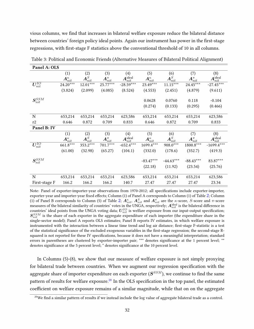
vious columns, we �nd that increases in bilateral welfare exposure reduce the bilateral distancebetween countries’ foreign policy ideal points. Again our instrument has power in the �rst-stageregressions, with �rst-stage F statistics above the conventional threshold of 10 in all columns.

Table 3: Political and Economic Friends (Alternative Measures of Bilateral Political Alignment)Panel A: OLS

(1) (2) (3) (4) (5) (6) (7) (8)A

nitAS

nitA⇡

nitAideal

nitA

nitAS

nitA⇡

nitAideal

nit

U IO

nit24.20⇤⇤⇤ 12.01⇤⇤⇤ 25.77⇤⇤⇤ -28.59⇤⇤⇤ 23.49⇤⇤⇤ 11.15⇤⇤⇤ 24.45⇤⇤⇤ -27.45⇤⇤⇤(3.824) (2.099) (4.085) (8.524) (4.553) (2.451) (4.879) (9.611)

SSSM

nit0.0628 0.0760 0.118 -0.104(0.274) (0.133) (0.295) (0.466)

N 653,214 653,214 653,214 623,586 653,214 653,214 653,214 623,586r2 0.646 0.872 0.709 0.833 0.646 0.872 0.709 0.833Panel B: IV

(1) (2) (3) (4) (5) (6) (7) (8)A

nitAS

nitA⇡

nitAideal

nitA

nitAS

nitA⇡

nitAideal

nit

U IOnit

661.8⇤⇤⇤ 353.2⇤⇤⇤ 701.7⇤⇤⇤ -652.4⇤⇤⇤ 1699.4⇤⇤⇤ 908.0⇤⇤⇤ 1800.8⇤⇤⇤ -1699.4⇤⇤⇤(61.00) (32.98) (65.27) (104.1) (332.0) (178.6) (352.7) (419.3)

SSSM

nit-83.47⇤⇤⇤ -44.63⇤⇤⇤ -88.43⇤⇤⇤ 83.87⇤⇤⇤(22.18) (11.92) (23.54) (25.76)

N 653,214 653,214 653,214 623,586 653,214 653,214 653,214 623,586First-stage F 166.2 166.2 166.2 140.7 27.47 27.47 27.47 23.34

Note: Panel of exporter-importer-year observations from 1970-2012; all speci�cations include exporter-importer,exporter-year and importer-year �xed e�ects; Column (1) of Panel A corresponds to Column (1) of Table 2; Column(1) of Panel B corresponds to Column (5) of Table 2; A

nit, AS

nitand A⇡

nitare the -score, S-score and ⇡-score

measures of the bilateral similarity of countries’ votes in the UNGA, respectively;Aidealnit

is the bilateral di�erence incountries’ ideal points from the UNGA voting data; U IO

nitis welfare exposure from our input-output speci�cation;

SSSM

nitis the share of each exporter in the aggregate expenditure of each importer (the expenditure share in the

single-sector model); Panel A reports OLS estimates; Panel B reports IV estimates, in which welfare exposure isinstrumented with the interaction between a linear time trend and log air distance; �rst-stage F-statistic is a testof the statistical signi�cance of the excluded exogenous variables in the �rst-stage regression; the second-stage R-squared is not reported for these IV speci�cations, because it does not have a meaningful interpretation; standarderrors in parentheses are clustered by exporter-importer pair; *** denotes signi�cance at the 1 percent level; **denotes signi�cance at the 5 percent level; * denotes signi�cance at the 10 percent level.

In Columns (5)-(8), we show that our measure of welfare exposure is not simply proxyingfor bilateral trade between countries. When we augment our regression speci�cation with theaggregate share of importer expenditure on each exporter (SSSM ), we continue to �nd the samepattern of results for welfare exposure.20 In the OLS speci�cation in the top panel, the estimatedcoe�cient on welfare exposure remains of a similar magnitude, while that on on the aggregate

20We �nd a similar pattern of results if we instead include the log value of aggregate bilateral trade as a control.

32

import share is statistically insigni�cant. In the IV speci�cation in the bottom panel, the estimatedcoe�cient on welfare exposure remains of the same sign and increases in absolute magnitude.In contrast, the estimated coe�cient on the aggregate import share has the opposite sign andis statistically signi�cant, which likely re�ects the fact that the aggregate import share itself isendogenous. We nevertheless report this speci�cation to show that our estimates for welfareexposure are not simply capturing bilateral trade between countries, which is consistent withthe discussion in Section 4.1, where we noted that our exposure measures are not completelycaptured by simpler measures of trading relationships between countries.

Alternative Measures of Bilateral Political Alignment While we have so far consideredmeasures of bilateral political alignment based on UNGA voting data, we now demonstrate therobustness of our results to the use of alternative measures of bilateral political alignment.

In Table 4, we estimate the same regression speci�cation (14) using our measures of strategicrivalry, which capture the contemporary perceptions of policy-makers as to whether two coun-tries regard each other as competitors, sources of threats or enemies. Columns (1)-(4) present theOLS estimates, while Columns (5)-(8) contain the IV estimates. Whether we consider all strategicrivalries (Columns (1) and (5)), positional strategic rivalries (Columns (2) and (6)), spatial strategicrivalries (Columns (3) and (7)) or ideological strategic rivalries (Columns (4) and (8)), we �nd thesame pattern of results. In all cases, we �nd a negative and statistically signi�cant relationshipbetween the propensity with which countries are strategic rivals and bilateral welfare exposure.Consistent with the UNGA voting results, when we instrument bilateral welfare exposure withour interaction between a linear trend and bilateral distance, we �nd an even stronger relation-ship, with an increase in the absolute magnitude of the estimated coe�cient. Again we �nd thatour instrument has power in the �rst-stage regression, as indicated by the �rst-stage F-statistic.

33

Table 4: Political and Economic Friends (Strategic Rivalries Speci�cation)(1) (2) (3) (4) (5) (6) (7) (8)

AAnynit

APosnit

ASpanit

AIdnit

AAnynit

APosnit

ASpanit

AIdnit

U IO

nit-3.234⇤⇤⇤ -0.851⇤⇤⇤ -1.191⇤⇤⇤ -1.912⇤⇤ -104.5⇤⇤⇤ -50.50⇤⇤⇤ -71.91⇤⇤⇤ -52.30⇤⇤⇤(1.100) (0.325) (0.446) (0.975) (22.72) (14.31) (18.17) (14.63)

Estimation OLS OLS OLS OLS IV IV IV IVN 788,396 788,396 788,396 788,396 779,664 779,664 779,664 779,664R-squared 0.791 0.837 0.807 0.729 � � � �First-stage F � � � � 164.2 164.2 164.2 164.2

Note: Panel of exporter-importer-year observations from 1970-2012; all speci�cations include exporter-importer,exporter-year and importer-year �xed e�ects; AAny

nit, APos

nitand ASpa

nitand AId

nitare indicator variables for any, po-

sitional, spatial and ideological strategic rivalries, respectively; U IO

nitis welfare exposure from our input-output

speci�cation; Columns (1)-(4) report OLS estimates; Columns (5)-(8) report IV estimates, in which welfare expo-sure is instrumented with the interaction between a linear time trend and log air distance; �rst-stage F-statistic is atest of the statistical signi�cance of the excluded exogenous variables in the �rst-stage regression; the second-stageR-squared is not reported for the IV speci�cations, because it does not have a meaningful interpretation; standard er-rors in parentheses are clustered by exporter-importer pair; *** denotes signi�cance at the 1 percent level; ** denotessigni�cance at the 5 percent level; * denotes signi�cance at the 10 percent level.

In Table 5, we re-estimate this regression speci�cation (14) using our measures of formalalliances between countries. The top panel reports the OLS estimates, while the bottom panelgives the IV estimates. We �nd the same pattern of results for any alliances (Column (1)), mutualdefense pacts (Column (2)), non-aggression treaties (Column (4)) and ententes (Column (5)). Con-sistent with the UNGA voting results, we �nd a positive and statistically signi�cant relationshipbetween the frequency with which countries form alliances and bilateral welfare exposure. Whenwe instrument bilateral welfare exposure with our interaction between a linear trend and bilat-eral distance, we again �nd that this relationship strengthens, with an increase in the absolutemagnitude of the estimated coe�cient. The only exception is for neutrality pacts, where the es-timated coe�cient is statistically insigni�cant in the OLS speci�cation, but becomes positive andstatistically signi�cant in the IV speci�cation. This pattern of results could re�ect the fact thatneutrality decisions are more tied to multilateral considerations (with all of a country’s neigh-bors) rather than bilateral considerations (with one of a country’s neighbors). Again we �nd thatour instrument has power in the �rst-stage regression, as shown by the �rst-stage F-statistic.

34

Table 5: Political and Economic Friends (Formal Alliances Speci�cation)

Panel A: OLS(1) (2) (3) (4) (5)

AAllAnynit

AAllDefnit

AAllNeunit

AAllNonnit

AAllEntnit

U IO

nit4.518⇤⇤⇤ 2.994⇤⇤ 0.986 3.734⇤⇤⇤ 3.949⇤⇤⇤(1.200) (1.257) (0.969) (1.448) (1.147)

N 788,396 788,396 788,396 788,396 788,396R-squared 0.899 0.902 0.564 0.897 0.908Panel B: IV

(1) (2) (3) (4) (5)AAllAny

nitAAllDef

nitAAllNeu

nitAAllNon

nitAAllEnt

nit

U IO

nit803.0⇤⇤⇤ 798.0⇤⇤⇤ 35.98⇤⇤⇤ 603.3⇤⇤⇤ 550.7⇤⇤⇤(74.43) (73.30) (12.38) (60.20) (54.30)

N 779,664 779,664 779,664 779,664 779,664First-stage F 164.2 164.2 164.2 164.2 164.2

Note: Panel of exporter-importer-year observations from 1970-2012; all speci�cations include exporter-importer,exporter-year and importer-year �xed e�ects; AAllAny

nit, AAllDef

nit, AAllNeu

nit, AAllNon

nit, and AAllEnt

nitare indicator variables

for any, defense, neutrality, non-aggression and entente formal alliances, respectively; U IO

nitis welfare exposure

from our input-output speci�cation; Panel A reports OLS estimates; Panel B reports IV estimates, in which welfareexposure is instrumentedwith the interaction between a linear time trend and log air distance; �rst-stage F-statistic isa test of the statistical signi�cance of the excluded exogenous variables in the �rst-stage regression; the second-stageR-squared is not reported for the IV speci�cations, because it does not have a meaningful interpretation; standarderrors in parentheses are clustered by exporter-importer pair; *** denotes signi�cance at the 1 percent level; **denotes signi�cance at the 5 percent level; * denotes signi�cance at the 10 percent level.

Long-Di�erences Speci�cation In our empirical results so far, we have used an exporter-importer-year panel, which allows us to include exporter-importer �xed e�ects to control fortime-invariant unobserved heterogeneity, and exporter-year and importer-year �xed e�ects tocontrol for the sign and magnitude of productivity growth and time-varying factors that arecommon across trade partners for each exporter and importer. Although this panel data speci�-cation focuses on changes in bilateral political alignment and welfare exposure within country-partner pairs, it uses deviations each year from the country-partner time mean, and one concerncould be that bilateral political alignment changes over longer-time horizons. Our IV speci�-cation addresses this concern, by using an interaction between a linear trend and distance asour instrument, which implies that we exploit variation from di�erences in linear trends withincountry-partner pairs between long versus short bilateral distances. As a further robustness checkto address this concern, Section G of the online appendix reports a long-di�erences speci�cationusing �ve-year di�erences. In this speci�cation, we di�erence out the exporter-importer �xede�ects, and again include exporter-year and importer-year �xed e�ects to control for the signand magnitude of productivity growth and time-varying factors that are common across trade

35

partners for each exporter and importer. Again in both our OLS and IV estimates, we �nd thatincreases in bilateral welfare exposure raise bilateral political alignment, con�rming the resultsof our baseline panel data speci�cation here.

Summary As a country becomes more economically exposed to productivity growth in a tradepartner, we �nd that it becomes more politically aligned with that trade partner. We �nd thispattern of results using quite di�erent approaches to measuring political alignment: (i) UnitedNations voting data; (ii) the perceptions of contemporary policy-makers about strategic rival-ries; and (iii) formal alliances between nations. We �nd this relationship after controlling forunobserved time-invariant heterogeneity that is speci�c to each country-partner pair (e.g. geo-graphical location and institutions) and time-varying factors that are speci�c to each exporter andimporter and common across trade partners. Our estimates therefore focus on changes in bilateralpolitical alignment and bilateral welfare exposure within individual country-partner pairs. Wedemonstrate that this relationship holds whether we use all of the observed variation in bilateralwelfare exposure (in our OLS speci�cation) or the di�erential changes in welfare exposure be-tween long and short bilateral distances because of improvements in the technology of air travel(in our IV speci�cation). Therefore, whether we consider China’s emergence into the global econ-omy as a natural experiment (previous section) or exogenous variation from the improvement inthe technology of air travel (this section), we �nd that increases in economic friendship lead toincreases in political friendship between countries.

5 Speci�cation Checks

In this section, we report additional speci�cation checks on our economic exposure measures.In Subsection 5.1, we report an overidenti�cation check on these measures, in which we showthat they are systematically related to separate data on preferential trade agreements (PTAs) thatwere not used in their estimation. In Subsection 5.2, we report a speci�cation check, in whichwe examine the potential role for non-linearities, by comparing the predictions of our lineariza-tion to the full non-linear model solution. We show that our exposure measures provide a goodapproximation to the full non-linear model solution for empirically-realistic shocks, includingcumulative changes in productivity over our sample period of more than forty years.

5.1 Preferential Trade Agreements (PTAs)

We use separate data on PTAs to provide an overidenti�cation check on our economic exposuremeasures. We �rst examine the determinants of PTAs: If our exposure measures correctly capturegains from economic integration, we would expect them to predict self-selection into PTAs. We

36

next examine the e�ects of PTAs: If our exposure measures correctly capture economic interde-pendence between countries, we would expect to observe systematic changes in these measuresfollowing the formation of PTAs.

In Section H.1.1 of the online appendix, we estimate a selection model for the decision to forma PTA. We show that initial income and welfare exposure to reductions in bilateral trade costsin 1970 are predictive of the subsequent formation of PTAs from 1971-2012. We show that thisresult is robust to controlling for simpler measures of trading relationships between countries,such as initial bilateral trade or aggregate expenditure shares in 1970, or geographical distance.In Section H.1.2 of the online appendix, we use an event-study speci�cation to provide evidenceon the e�ects of PTAs. We show that our exposure measures successfully detect increases ineconomic interdependence between member countries following the formation of PTAs. We �ndthis pattern of results whether we use exposure to productivity growth or bilateral trade costreductions, and after controlling for simpler measures of trading relationships between countries.We demonstrate that these results hold across a range of di�erent event-study speci�cations,including those that allow for variable timing of the treatment and treatment heterogeneity.

Therefore, we �nd that our exposure measures have predictive power for separate data onPTAs not used in their estimation, both in terms of predicting selection into future PTAs, andin terms of detecting the impact of these future PTAs in increasing economic interdependencebetween countries.

5.2 Non-linearities

In Section 2, we derived our measures of the sensitivity of country income and welfare to for-eign productivity growth from a linearization of the class of international trade models with aconstant trade elasticity. We now report a speci�cation check in which we examine the poten-tial role for non-linearities by comparing the predictions of our linearization to those of the fullnon-linear model solution. To build intuition, we �rst compare the two approaches in our base-line single-sector model, before implementing this comparison for our quantitative speci�cationwith multiple sectors and input-output linkages. We focus largely on the quality of our approx-imation to the full non-linear model solution for productivity shocks that are the subject of ourempirical application. For completeness, we also report some results comparing the quality ofour approximation for trade cost shocks.

5.2.1 Single-Sector Model

As discussed above, a �rst key advantage of our representation of the �rst-order general equilib-rium e�ect of productivity shocks in terms of the expenditure share (S), income share (T ) andcross-substitution (M ) matrices is that it can be used to provide an analytical characterization

37

of the quality of the �rst-order approximation to the full non-linear model solution in terms ofthese observed matrices.

In Section H.2.1 of the online appendix, we show that the di�erence between the predictionsof our linearization and the full non-linear model solution for the impact of productivity shockscorresponds to the di�erence between the log of a weighted mean and a weighted mean of logs.This di�erence corresponds to the second and higher-order terms in a Taylor-series expansionaround the initial equilibrium. We show that this di�erence is necessarily equal to zero in thetwo limiting cases of autarky (tnn ! 1 and snn ! 1 for all n) and free trade (tin ! ti andsni ! si for all n, i). More generally, in Propositions A.2-A.6 in Section H.2.2 of the onlineappendix, we use this Taylor-series expansion to derive analytical global bounds of the absolutemagnitude of the second and higher-order terms in terms of the observed expenditure share (S),income share (T ) and cross-substitution (M ) matrices. Given these observed trade matrices anda central value for the trade elasticity of ✓ = 5, we show that the global approximation errorsfor the absolute magnitude of the second and higher-order terms are less than 0.62 percent of thevariance of productivity shocks for income exposure, and less than 0.33 percent of the varianceof productivity shocks for welfare exposure.

At �rst glance, these results appear to contrast with the �ndings in Baqaee and Farhi (2019)that second-order terms can be large in response to economic shocks. However, our results arederived for the in�uential class of trade models with a single constant trade elasticity, whereasthe Baqaee and Farhi (2019) results are derived for a general network economy and illustratedusing the example of a nested constant elasticity of substitution (CES) economy. It is preciselythe presence of the multiple CES nests with di�erent elasticities of substitution in this examplethat generates the large second-order terms, whereas in speci�cations with a single elasticity ofsubstitution, these second-order terms remain small.

5.2.2 Multiple Sectors and Input-Output Linkages

A second key advantage of our our representation of the �rst-order general equilibrium ef-fect of productivity shocks in terms of the expenditure share (S), income share (T ) and cross-substitution (M ) matrices is that this same representation holds across a wide range of trademodels, after making appropriate changes to the elements of these matrices. We now implementthis comparison of our linearization and the full non-linear model solution for our state of the artquantitative speci�cation with multiple sectors and input-output linkages.

Empirical Distributions of Productivity and Trade Cost Shocks We begin by recoveringempirical distributions of productivity and trade cost shocks that we use to compare the predic-tions of the two approaches. Since we undertake counterfactuals for productivity and trade cost

38

shocks that are common across sectors, we recover these empirical distributions of shocks fromour single-sector model, as discussed in Section H.2.4 of the online appendix. In Figure 7, we dis-play histograms of the resulting log changes in relative productivity (left panel) and trade costs(right panel) for our sample period as a whole, based on our central value of the trade elasticity of✓ = 5. We normalize both variables to have a mean of zero in logs. The distribution of productiv-ity shocks is across countries, while the distribution of trade cost shocks is across country-partnerpairs. Over this period of more than forty years, which includes double-digit annual growth forsome countries such as China, we �nd large changes in both relative productivity and trade costs.Relative changes in productivity span close to 20 log points (from -9 to 10 log points), while rel-ative changes in trade costs span 10 log points (from -5 to 5 log points). Therefore, although wecould undertake counterfactuals in the non-linear model using any distributions of productiv-ity and trade cost shocks, these empirical distributions provide ample variation to examine theimportance of non-linearities.

Figure 7: Empirical Distributions of Productivity and Trade Cost Shocks from 1970-2012

-10 0 10Productivity shocks (log points)

0

0.1

0.2

0.3

0.4

Den

sity

-5 0 5Trade cost shocks (log points)

0

0.05

0.1

Den

sity

Note: Empirical distributions (histograms) of log productivity shocks (left panel) and log trade cost shocks (rightpanel) from 1970-2012; productivity and trade cost shocks recovered from inverting the single-sector model, asshown in Section H.2.4 of the online appendix. Both log productivity and trade costs shocks are normalized to havea mean of zero, so that the �gure shows shocks to relative productivity and relative trade costs.

Productivity and Trade Cost Shocks We use these empirical distributions of productivityand trade cost shock to undertake counterfactuals in the non-linear model with multiple sectorsand input-output linkages. In particular, we compare the predictions of conventional exact-hatalgebra counterfactuals in the non-linear model to the predictions of our linearization, which canbe recovered by multiplying our exposure measures by the size of the productivity or trade costshock. We begin by undertaking this comparison for our central value of the trade elasticity of✓ = 5. We vary the magnitude of the productivity shocks by taking weighted averages of thevector of empirical shocks from 1970-2012 in Figure 7 and a vector of ones that corresponds to

39

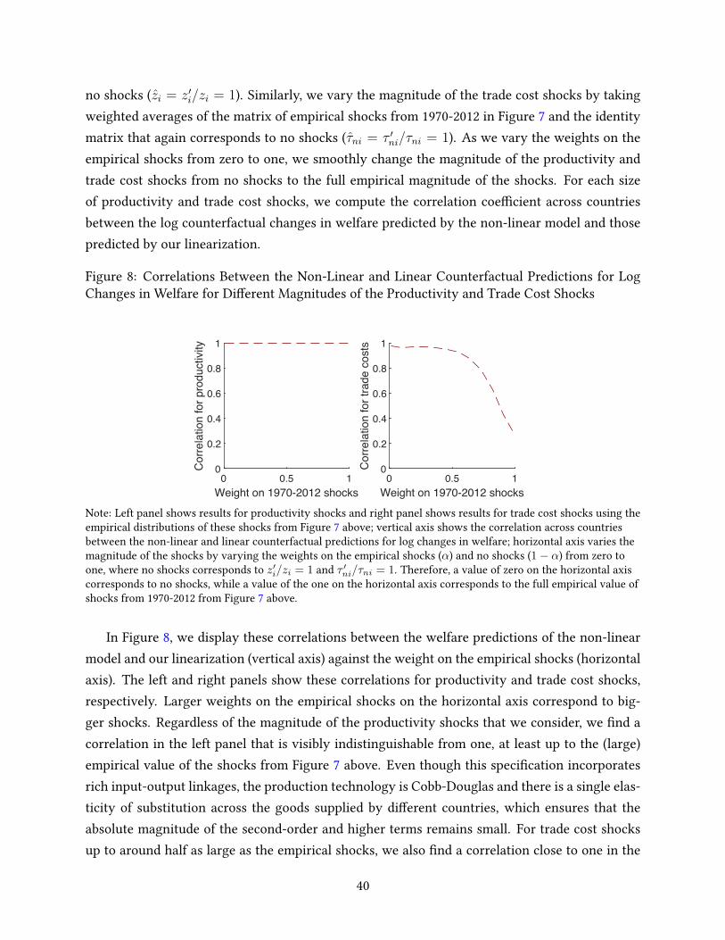
no shocks (zi = z0i/zi = 1). Similarly, we vary the magnitude of the trade cost shocks by taking

weighted averages of the matrix of empirical shocks from 1970-2012 in Figure 7 and the identitymatrix that again corresponds to no shocks (⌧ni = ⌧ 0

ni/⌧ni = 1). As we vary the weights on the

empirical shocks from zero to one, we smoothly change the magnitude of the productivity andtrade cost shocks from no shocks to the full empirical magnitude of the shocks. For each sizeof productivity and trade cost shocks, we compute the correlation coe�cient across countriesbetween the log counterfactual changes in welfare predicted by the non-linear model and thosepredicted by our linearization.

Figure 8: Correlations Between the Non-Linear and Linear Counterfactual Predictions for LogChanges in Welfare for Di�erent Magnitudes of the Productivity and Trade Cost Shocks

0 0.5 1Weight on 1970-2012 shocks

0

0.2

0.4

0.6

0.8

1

Cor

rela

tion

for t

rade

cos

ts

0 0.5 1Weight on 1970-2012 shocks

0

0.2

0.4

0.6

0.8

1

Cor

rela

tion

for p

rodu

ctiv

ity

Note: Left panel shows results for productivity shocks and right panel shows results for trade cost shocks using theempirical distributions of these shocks from Figure 7 above; vertical axis shows the correlation across countriesbetween the non-linear and linear counterfactual predictions for log changes in welfare; horizontal axis varies themagnitude of the shocks by varying the weights on the empirical shocks (↵) and no shocks (1� ↵) from zero toone, where no shocks corresponds to z0

i/zi = 1 and ⌧ 0

ni/⌧ni = 1. Therefore, a value of zero on the horizontal axis

corresponds to no shocks, while a value of the one on the horizontal axis corresponds to the full empirical value ofshocks from 1970-2012 from Figure 7 above.

In Figure 8, we display these correlations between the welfare predictions of the non-linearmodel and our linearization (vertical axis) against the weight on the empirical shocks (horizontalaxis). The left and right panels show these correlations for productivity and trade cost shocks,respectively. Larger weights on the empirical shocks on the horizontal axis correspond to big-ger shocks. Regardless of the magnitude of the productivity shocks that we consider, we �nd acorrelation in the left panel that is visibly indistinguishable from one, at least up to the (large)empirical value of the shocks from Figure 7 above. Even though this speci�cation incorporatesrich input-output linkages, the production technology is Cobb-Douglas and there is a single elas-ticity of substitution across the goods supplied by di�erent countries, which ensures that theabsolute magnitude of the second-order and higher terms remains small. For trade cost shocksup to around half as large as the empirical shocks, we also �nd a correlation close to one in the

40

right panel. As we increase the magnitude of the trade cost shocks towards the (large) empiricalvalue of the shocks, we �nd that the correlation begins to fall, but it remains above 0.5 for most ofthe interval, and is always positive and statistically signi�cant at conventional levels.21 Even forlarge trade cost shocks for which the correlation falls, we �nd that this decline is driven by a fewcountries, and that for most countries the linear and non-linear predictions for the log changesin welfare are close, as shown in Section H.2.6 of the online appendix.

Robustness to Alternative Trade Elasticities (✓ 2 [2, 20]) So far, we have established astrong correlation between the linear and non-linear predictions for the productivity shocks thatare the subject of our empirical application using a central trade elasticity of ✓ = 5. We nowdemonstrate the robustness this result to the assumption of alternative values for the trade elas-ticity from 2 to 20, which spans the empirically-relevant range.22 We use the full empirical mag-nitude of productivity shocks at the right-most point on the horizontal axis in Figure 8 witha weight of one. We hold the empirical distribution of productivity shocks constant and com-pute the correlation between the linear and non-linear predictions for log changes in welfare inresponse to these productivity shocks for alternative values of the trade elasticity. Across theentire of this empirically-relevant range of trade elasticities, we �nd a correlation close to one.As we increase the trade elasticity, the correlation between the linear and non-linear predictionsincreases, because for larger trade elasticities smaller changes in the endogenous variables arerequired to restore equilibrium in the model in response to the productivity shocks.

Therefore, for the sensitivity of country welfare to productivity shocks that is the subject ofour empirical application, our exposure measures closely approximate the full non-linear modelsolution for empirically-realistic shocks across the entire range of empirically-relevant values forthe trade elasticity from 2 to 20, even when we consider cumulative changes in productivity overour sample period of more than forty years. An advantage of our linearization relative to the fullnon-linear model solution is that our exposure measures can be computed from observed tradedata alone, thereby avoiding the challenge of measuring counterfactual shocks that in�uencedcountry behavior but did not occur.

21Whereas productivity shocks are common across all trade partners, trade shocks are bilateral, which resultsin a three-tensor rather than a matrix representation (see Section D.1 of the online appendix). Our friend-enemyrepresentation reduces this three-tensor down to a matrix using the observed trade shares, which contributes to thelower correlation between the non-linear and linear predictions for large changes in trade costs.

22Eaton and Kortum (2002) reports estimates of the trade elasticity ranging from 2 to 12; Costinot and Rodríguez-Clare (2014) assumes a central value of 5; and Simonovska and Waugh (2014) estimates a value of 4.

41

Figure 9: Correlations Between the Non-Linear and Linear Counterfactual Predictions for LogChanges in Welfare in Response to Productivity Shocks for Trade Elasticities from 2 to 20

0 5 10 15 20Trade Elasticity

0.99994

0.99996

0.99998

1

Cor

rela

tion

for p

rodu

ctiv

ity

Note: Vertical axis shows the correlation across countries between the linear and non-linear counterfactualpredictions for log changes in welfare in response to the full empirical magnitude of productivity shocks from1970-2012 from Figure 7 above; horizontal axis shows the trade elasticity (✓).

6 Conclusions

To what extent do nations’ economic interests in�uence their political behavior? We provide newevidence on this question using network measures of the sensitivity of welfare in one countryto productivity growth in another country. We propose a bilateral friends-and-enemies matrixrepresentation of the �rst-order general equilibrium e�ect of productivity growth in one countryon welfare in another: One country is a friend [enemy] for income or welfare in another countryif its productivity growth raises [reduces] the income or welfare of the other country.

Our exposure measures have a number of advantages for studying the relationship betweenpolitical behavior and economic interests. First, they correspond exactly to the sensitivity of coun-try welfare with respect to foreign productivity growth in the class of constant elasticity trademodels. Second, they use only data on observed trade �ows, which avoids the challenge of mea-suring counterfactual shocks that in�uenced country behavior but did not in fact occur. Third,we recover the entire bilateral network of country income and welfare exposure to productivitygrowth, which allows us to use techniques from the networks literature to characterize the roleof countries’ positions in the network in in�uencing the e�ects of productivity growth. Fourth,we show that the same representation of our exposure measures in terms expenditure share, in-come share and cross-substitution matrices holds across a wide range of trade models, includingspeci�cations with multiple sectors and input-output linkages, with appropriate changes to theelements of these matrices. Finally, we show that our representation can be used to provide ananalytical characterization of the quality of the �rst-order approximation to the full non-linearmodel solution in terms of these observed matrices.

42

We combine our economic exposure measures with data on bilateral political alignment thatcapture softer forms of political power beyondmilitary con�ict. We use two sources of exogenousvariation to provide evidence on the relationship between countries’ political behavior and theireconomic interests. First, following China’s market-orientated reforms in 1978, we show thatother countries realign politically towards China and away from the United States. We showthat this political realignment is greater in countries that experience larger increases in welfareexposure to China relative to the United States, consistent with the idea that economic interestsshape political behavior. To further strengthen the evidence in support of this relationship, we useour network measure of countries’ initial hub scores in 1980 shortly after China’s liberalization.We show that the countries with the highest initial levels of exposure to productivity growthin any nation experience the largest political realignment towards China relative to the UnitedStates, consistent with these countries being the most vulnerable to the change in relative welfareexposure following China’s emergence into the global economy.

Second, we make use of the large-scale reduction in the cost of air travel that occurred overour sample period, which reduced bilateral trade costs for some exporter-importer pairs by morethan for others. By exploiting this variation in trade costs over time within exporter-importerpairs, we control for a host of time-invariant factors that are speci�c to individual pairs of coun-tries (e.g. geographical location, institutions, legal origin, common language etc.). We also includeexporter-year and importer-year �xed e�ects, which control for the sign and absolute magnitudeof actual or expected exporter productivity growth, as well as policy changes that are common toall trade partners andmacro shocks. Using these di�erential changes in relative trade costs withinexporter-importer pairs, we again �nd that increases in bilateral welfare exposure raise bilateralpolitical alignment. We show that these results are robust across a range of econometric spec-i�cations (including panel and long-di�erences regressions) and measures of bilateral politicalalignment (including UN voting, strategic rivalries and formal alliances).

Therefore, using these two quite di�erent sources of quasi-experimental variation, we �nd thesame pattern of results, where as a country becomes more economically dependent on a tradepartner, it realigns politically towards that trade partner.

ReferencesA��, D., S. J��, �� J. R�� (2001): “The Colonial Origins of Comparative De-

velopment: An Empirical Investigation,” American Economic Review, 91, 1369–1401.A��, R., C. A��, �� F. E�� (2019): “Spatial Linkages, Global Shocks, and Local

Labor Markets: Theory and Evidence,” NBER Working Paper, 25544.A��, P., X. J��, T. P��, �� D. R�� (2018): “Education and Military Rivalry,”

Journal of the European Economic Association, 17, 376–412.A��, A. �� E. S�� (2003): The Size of Nations, Cambridge MA: MIT Press.

43

A��, T., C. A��, �� Y. T�� (2020): “Universal Gravity,” Journal of Political Econ-omy, 128, 393–433.

A��, J. E. �� E. �� W�� (2003): “Gravity with Gravitas: A Solution to the BorderPuzzle,” American Economic Review, 93, 170–192.

A��, C., A. C��, �� A. R��C�� (2012): “New Trade Models, Same OldGains,” American Economic Review, 102, 94–130.

A��, P. S. (1969): “A Theory of Demand for Products Distinguished by Place of Produc-tion,” IMF Sta� Papers, 16, 159–178.

A��, D., D. D��, �� G. H. H�� (2013): “The China Syndrome: Local Labor MarketE�ects of Import Competition in the United States,” American Economic Review, 103, 2121–68.

B��, M. A., A. S��, �� E. V�� (2017): “Estimating Dynamic State Preferencesfrom United Nations Voting Data,” Journal of Con�ict Resolution, 61, 430–456.

B��, X., Q. L��, L. D. Q��, �� D. Z�� (2019): “The E�ects of Bilateral Attitudes on Imports,”Shanghai University of Finance and Economics.

B��, D. R. �� E. F�� (2019): “Networks, Barriers, and Trade,” Harvard University.B��, K. (2002): The Liberal Illusion, Does Trade Promote Peace, Ann Arbor: University of

Michigan Press.B��, J. (1958): “Immiserizing Growth: A Geometrical Note,” Review of Economic Studies, 25,

201–205.B��, S. �� G. H�� (2006): “How Much Does Violence Tax Trade,” Review of Economics

and Statistics, 88, 599–612.B��, M., R. D��, �� H. J�� (2018): “Beijing’s Bismarckian Ghosts: How Great

Powers Compete Economically,” The Washington Quarterly, 41, 161–176.C��, L., M. D��, �� F. P�� (2019): “Trade and Labor Market Dynamics: General

Equilibrium Analysis of the China Trade Shock,” Econometrica, 87, 741–835.C��, L. �� F. P�� (2015): “Estimates of the Trade andWelfare E�ects of NAFTA,” Review

of Economic Studies, 82, 1–44.C��, J. (1960): “A Coe�cient of Agreement for Nominal Scales,” Educational and Psychological

Measurement, 20, 37–46.C��, M. P., K. R��, �� W. R. T�� (2010): Strategic Rivalries in World Politics:

Position, Space and Con�ict Escalation, Cambridge University Press.C��, A., D. D��, �� I. K�� (2012): “What Goods Do Countries Trade? A

Quantitative Exploration of Ricardo’s Ideas,” Review of Economic Studies, 79, 581–608.C��, A. �� A. R��C�� (2014): “Trade Theory with Numbers: Quantifying the

Consequences of Globalization,” in Handbook of International Economics, ed. by G. Gopinath,E. Helpman, and K. Rogo�, Amsterdam: Elsevier North-Holland, vol. 4, chap. 4, 197–261.

�� M��, B. B. �� R. M. S�� (1995): “War and the Survival of Political Leaders: AComparative Study of Regime Types and Political Accountability,” American Political ScienceReview, 89, 841–855.

D��, A. ��M. V. S�� (2018): “Agree to Disagree: The Spillover of Trade Policy intoUnited Nations Assembly Voting,” UNCTAD Research Paper, 28.

E��, J. �� S. K�� (2002): “Technology, Geography, and Trade,” Econometrica, 70, 1741–1779.

E��, T. �� D. S�� (2007): “News Droughts, News Floods, and US Disaster Relief,”Quarterly Journal of Economics, 122, 693–728.

F��, R. C., R. E. L��, H. D��, A. C. M�, �� H. M� (2005): “World Trade Flows: 1962-2000,” NBER Working Paper, 11040.

F��, J. (2019): “Trade and Income� Exploiting Time Series in Geography,” American EconomicJournal: Applied Economics, 11, 1–35.

F��, J. A. ��D. H. R�� (1999): “Does Trade Cause Growth?” American Economic Review,

44

89, 379–399.G��, E. (2007): “The Capitalist Peace,” American Journal of Political Science, 51, 166–191.G��, D. M. (2008): International Military Alliances, 1648-2008, CQ Press.G��, R. �� A. M. T�� (2010): “Collateral Damage: Trade Disruption and the Economic

Impact of War,” Review of Economics and Statistics, 92, 102–127.G��, L., P. S��, �� L. Z�� (2009): “Cultural Biases in Economic Exchange,” Quar-

terly Journal of Economics, 124, 1095–1131.H��, F. M. (2011): “Choice or Circumstance? Adjusting Measures of Foreign Policy Similarity

for Chance Agreement,” Political Analysis, 19, 287–305.H��, K. �� T. M�� (2013): “What Separates Us? Sources of Resistance to Globalization,”

Canadian Journal of Economics, 46, 1196–1231.H��, K., T. M��, �� J. R�� (2010): “The Erosion of Colonial Trade Linkages after Indepen-

dence,” Journal of International Economics, 81, 1–14.H��, J. (1953): “An Inaugural Lecture,” Oxford Economic Papers, 5, 117–135.H��, C., A. O��, �� M. R�� (2017): “Horizontal Depth: A New Database on the

Content of Preferential Trade Agreements,”World Bank Policy Research Working Paper, 7981.H��, D. (2007): “Transportation Costs and International Trade in the Second Era of Global-

ization,” Journal of Economic Perspectives, 21, 131–54.H��, Z., A. A. L��, �� N. P��N�� (2019): “International Comovement in the

Global Production Network,” NBER Working Paper, 25978.J��, H. (1955): “Economic Expansion and International Trade,” The Manchester School, 23,

95–112.J��, R. W. �� J. S�� (1977): “The Relevance of the Two-Sector Production Model in

Trade Theory,” Journal of Political Economy, 85, 909–935.K��, J. (1999): “Authoritative sources in a hyperlinked environment,” Journal of the ACM.K��, M. D., D. R��, M. T��, �� F. Z�� (2017): “Networks in Con�ict: Theory

and Evidence from the Great War of Africa,” Econometrica, 85, 1093–1132.K��, I. �� E.W�� (2006): “HowMuch is a Seat on the Security CouncilWorth? Foreign

Aid and Bribery at the United Nations,” Journal of Political Economy, 114, 905–930.M��, E. (1995): Power, Trade and War, Princeton: Princeton University Press.M��, P., T. M��, �� M. T�� (2008): “Make Trade Not War?” Review of Economic

Studies, 75, 865–900.M��, E., G. P�� M��, �� N. Q�� (2008): “The Rise of China and the Natural

Resource Curse in Africa,” Northwestern University, mimeograph.N��, N. �� N. Q�� (2014): “US Food Aid and Civil Con�ict,” American Economic Review, 104,

1630–1666.N��, J. S. (1990): “Soft Power,” Foreign Policy, 80, 153–171.P��, A. (1984): “Econometric Issues in the Analysis of Regressions with Generated Regressors,”

International Economic Review, 25, 221–247.P��, S. (1980): “Con�ict and Trade,” Journal of Con�ict Resolution, 24, 57–78.R��, F. �� D. R�� (2001): “Trade Policy and Economic Growth: A Skeptic’s Guide to

the Cross-National Evidence,” NBER Macroeconomics Annual, 15, 261–338.S�� S��, J. M. C. �� S. T�� (2006): “The Log of Gravity,” Review of Economics and

Statistics, 88, 641–658.S��, W. A. (1955): “Reliability of Content Analysis: The Case of Nominal Scale Coding,” The

Public Opinion Quarterly, 19, 321–5.S��, C. S. �� J. M. R�� (1999): “Tau-b or not tau-b: Measuring the Similarity of Foreign

Policy Positions,” International Studies Quarterly, 43, 115–44.S��, I. �� M. E. W�� (2014): “The Elasticity of Trade: Estimates and Evidence,”

45

Journal of International Economics, 92, 34–50.T��, W. R. (2001): “Identifying Rivals and Rivalries in World Politics,” International Studies

Quarterly, 45, 557–586.W��, C. A. (1980): “On the General Structure of RicardianModels with a Continuum of Goods:

Applications to Growth, Tari� Theory, and Technical Change,” Econometrica, 48, 1675–1702.

46

IFE Paper - Princeton University

Documents

Transcript of IFE Paper - Princeton University