IEEETRANSACTIONS ON INTELLIGENT TRANSPORTATION SYSTEMS 1

This article has been accepted for inclusion in a future issue of this journal. Content is final as presented, with the exception of pagination.

IEEE TRANSACTIONS ON INTELLIGENT TRANSPORTATION SYSTEMS 1

Learning the Dynamics of Arterial Traffic FromProbe Data Using a Dynamic Bayesian Network

Aude Hofleitner, Ryan Herring, Pieter Abbeel, and Alexandre Bayen

Abstract—Estimating and predicting traffic conditions in arte-rial networks using probe data has proven to be a substantial chal-lenge. Sparse probe data represent the vast majority of the dataavailable on arterial roads. This paper proposes a probabilisticmodeling framework for estimating and predicting arterial travel-time distributions using sparsely observed probe vehicles. Weintroduce a model based on hydrodynamic traffic theory to learnthe density of vehicles on arterial road segments, illustrating thedistribution of delay within a road segment. The characterizationof this distribution is essentially to use probe vehicles for traffic es-timation: Probe vehicles report their location at random locations,and the travel times between location reports must be properlyscaled to match the map discretization. A dynamic Bayesian net-work represents the spatiotemporal dependence on the networkand provides a flexible framework to learn traffic dynamics fromhistorical data and to perform real-time estimation with streamingdata. The model is evaluated using data from a fleet of 500 probevehicles in San Francisco, CA, which send Global PositioningSystem (GPS) data to our server every minute. The numericalexperiments analyze the learning and estimation capabilities on asubnetwork with more than 800 links. The sampling rate of theprobe vehicles does not provide detailed information about thelocation where vehicles encountered delay or the reason for anydelay (i.e., signal delay, congestion delay, etc.). The model providesan increase in estimation accuracy of 35% when compared with abaseline approach to process probe-vehicle data.

Index Terms—Expectation–maximization algorithms, probes,queuing analysis, real-time systems, statistical learning.

I. INTRODUCTION AND BACKGROUND

TRAFFIC congestion has a significant impact on economicactivity. An essential step toward active congestion control

is the creation of accurate reliable traffic monitoring systems,leveraging the latest advances in technology and research. His-torically, traffic monitoring systems have been mostly limited

Manuscript received September 21, 2011; revised February 9, 2012; acceptedMay 11, 2012. This work was supported in part by the Federal and CaliforniaDepartments of Transportation, by Nokia, by NAVTEQ, and by Cabspotting.The Associate Editor for this paper was S. Sun.

A. Hofleitner is with Partners for Advanced Transportation Technology,University of California, Berkeley, Berkeley, CA 94720-3830 USA (e-mail:[email protected]).

R. Herring was with the California Center for Innovative Transportation,University of California, Berkeley, Berkeley, CA 94720-3830 USA. He isnow with Apple Inc., Cupertino CA 95014 USA (e-mail: [email protected]).

P. Abbeel and A. Bayen are with the Department of Electrical Engineeringand Computer Sciences, University of California, Berkeley, Berkeley, CA94720-3830 USA (e-mail: [email protected]; [email protected]).

Color versions of one or more of the figures in this paper are available onlineat http://ieeexplore.ieee.org.

Digital Object Identifier 10.1109/TITS.2012.2200474

Fig. 1. Probe measurements in San Francisco, CA. The small (resp. large) dotsrepresent the measurement of the location of a taxi, received between midnightand 7 A.M. (resp. at 7 A.M.).

to highways and have relied on data feeds from a dedicatedsensing infrastructure (loop detectors, radars, etc.). For highwaynetworks covered by such an infrastructure, it is commonpractice to perform both system identification (free-flow speed,traffic jam density, and flow capacity) and estimation of trafficstate (flow, density, bulk speed, and shockwave location) at avery fine spatiotemporal scale [5], [46]. These highway trafficmonitoring approaches rely upon both the ubiquity of data andhighway traffic flow models developed over the last half century[11], [38].

For arterials, traffic monitoring is substantially more difficult:Probe-vehicle data are the only significant data source availabletoday with the prospect of global coverage in the future. Itcomes from various sources such as fleet vehicles periodicallyreporting their location (a rate of 1 min is currently the stan-dard), smartphones, aftermarket devices, or radio-frequencyidentification tags. The features of probe-vehicle data today,including the lack of ubiquity and a uniform penetration rate(the percentage of vehicle reporting their location varies acrossthe network and throughout the day), the variety of data typesand specifications, and the randomness of its spatiotemporalcoverage, make it insufficient for fully characterizing macro-scopic traffic model parameters and doing state estimation forlarge transportation networks. Fig. 1 shows the probe measure-ments collected on a day from midnight to 7 A.M. by one ofthe feeds of the Mobile Millennium system. It also shows asnapshot of the location of probes at 7 A.M. The figure showsboth the breadth of coverage when aggregating data over longperiods of time and the limited information available at a given

1524-9050/$31.00 © 2012 IEEE

mailto:[email protected]




2 IEEE TRANSACTIONS ON INTELLIGENT TRANSPORTATION SYSTEMS

point in time, limiting the direct estimation capabilities at afine spatiotemporal scale. Traffic models and data assimilationalgorithms must be developed to efficiently transform these datainto reliable traffic information (see, e.g., [28], [35], [44], and[46] for a discussion on the use of cell phone data for highwaytraffic monitoring).

Aside from less abundant sensing compared with exist-ing highway traffic monitoring systems, the arterial networkpresents additional modeling and estimation challenges: Theunderlying flow physics that governs them is more complexbecause of traffic lights (often with unknown cycles), intersec-tions, and others [8], [37]. Collecting the detailed parameters ofthe arterial road network into an accessible electronic databasewould require the cooperation of numerous government agen-cies, making this information unreliable and tedious to obtain.This makes the detailed spatiotemporal modeling and esti-mation approaches developed for highway traffic impracticalfor arterials, i.e., at least until the data volume significantlyincreases [3], [42], [45].

We are interested in a statistical approach to arterial trafficestimation based on Dynamic Bayesian Networks (DBNs).The model characterizes the variability of travel times amongvehicles traveling on the network and the stochasticity ofcongestion dynamics on arterial networks. Our approach isadapted to the only significant data source available today forarterial estimation: sparse measurements from probe-vehicledata. We present a brief overview of existing research focusedon statistical approaches for traffic estimation and underline thecontributions of this paper. An extended review of the literatureis available in [20]. Previous research has studied the estimationand short-term prediction of sensor readings using DBNs [36],[43] and regression models [40]. These articles assume thatsensors (such as loop detectors) provide measurements with afixed frequency at fixed locations. Probe data on arterials areavailable at random times and random locations, making thisassumption not applicable for this paper. Other approaches [16],[22] assume that either a single measurement per time intervalor aggregated measurements per time interval are availablefor each road segment of the network (according to the mapdiscretization). This assumption limits the capacity to representthe variability of travel times among the vehicles traveling onthe network. Moreover, such approaches are not adapted tomissing data, when no information is available on some partsof the network. An approach inspired from the Ising modelwas developed in [16]. It relies on binary measurements statingwhether traffic is congested or uncongested that are not directlyavailable from traffic sensors. Transforming traffic data intobinary congested/uncongested values is a difficult process byitself and has not been specifically addressed in the literatureto our knowledge. Our model offers such a binary quantizationfrom probe-vehicle travel times. Neural networks and patternmatching [12] have been used to estimate traffic from GlobalPositioning System (GPS) data under the critical assumptionthat the velocity is spatially homogeneous and similar amongdrivers. This assumption does not take into account the vari-ability of travel times due to the frequent stops at traffic signals.High-frequency probe data (one measurement approximatelyevery 20 s or less) [29] allow for reliable calculation of short-

distance speeds and travel times. In this paper, we specificallyaddress the processing of sparse probe data where this level ofgranularity is not available. Numerous estimation algorithmsfrom probe-vehicle data rely on the decomposition of pathtravel times to individual road segments, also referred to as links[19], [23]. However, when a vehicle travels more than one link,the location of its delay is unknown, and this decompositioncan lead to inaccuracies. In this paper, we use probe-vehicledata without the use of a travel-time decomposition algorithm.

The contribution of this paper specifically addresses theestimation and short-term forecast of the probability distribu-tion function (pdf) of travel times in the case of noisy sparseprobe data. In particular, we propose a model and an algorithmfor traffic estimation with measurements received at randomlocations and random times, which are based on the learningof the dynamics of congestion on the network. Each observa-tion, which is defined as two consecutive GPS measurementsincluding the travel time between these measurements, has aprobability density that depends on 1) the pdf of travel times ofthe links traversed and 2) the spatial distribution of vehicles oneach traversed link. The key insight is that, on average, vehi-cles are more likely to experience delay close to intersectionsbecause of the presence of traffic signals. We assume that thepdf of travel times on each link of the network depends on thelevel of congestion (congestion state) of this link, and we modeland learn the dynamics of congestion on the network using aDBN. We define a link as the road segment between signalizedintersections; however, this choice of discretization can be morefine if desired.

This paper is organized as follows. Section II presentsa graphical model representing the dependence between thetravel-time observations and the congestion state of eachlink at each time interval and their spatiotemporal evolution.Section III uses queuing theory to formalize the intuition thatvehicles are more likely to experience delays close to intersec-tions. We discuss how this information can be used to computethe pdf of travel times on an arbitrary path from the pdf oftravel times of the links traversed. Leveraging the modelingassumptions of Section II and the results from Section III, theDBN represents the probabilistic dynamics of traffic congestionand the probabilistic observation model of the congestion statesfrom probe data. We develop an expectation–maximization(EM) algorithm (see Section IV) for learning the parametersof the DBN. We perform the expectation step (E step) usingparticle filtering and solve a large convex optimization prob-lem using an interior point method for the maximization step(M step). After the historical learning of the parameters ofthe system’s dynamics, we estimate the current state of thenetwork and predict the probability of congestion and the pdfof link travel times from the probe data available in real time.Finally, we present the results of a case study (see Section V) inSan Francisco, CA, for which a fleet of 500 probe vehiclesprovides sparse location measurements [1]. These data are oneof the feeds available in the Mobile Millennium system [4].The system provides real-time streaming data and a history ofthe data collected since October 2009. The initial results indi-cate that travel-time distributions can be accurately estimatedusing sparse GPS data only.


HOFLEITNER et al.: LEARNING DYNAMICS OF ARTERIAL TRAFFIC FROM PROBE DATA USING DBN 3

II. TRAFFIC MODELING ASSUMPTIONS

A. Dynamical Model

Arterial traffic can be viewed as a dynamic stochastic pro-cess. Our model represents the main characteristics of traf-fic dynamics while making assumptions necessary for thetractability of the estimation process. The validity and limita-tion of the model are further discussed in Section VI, where wealso analyze how the model can be refined or generalized.

1) Time discretization: We model traffic as a discrete-timedynamical system. We call Δ the time discretization,which is chosen depending on the data available andthe desired temporal scale of the estimation. This paperis focused on estimating travel-time distributions whenmeasurements are sparse. We choose Δ to be equal to5 min in the numerical experiments as we are inter-ested in estimating trends rather than fluctuations. Fort ∈ T = {0, . . . , (T − 1)}, time interval t is given by[t0 + tΔ, t0 + (t+ 1)Δ].

2) Characterization of the state of traffic: For each linki ∈ I (I is the set of link indices), traffic conditions arecharacterized by a discrete random variable (RV) ξi,t. Wedenote by si,t ∈ {0, . . . , S − 1} the realization of the RVξi,t, representing a discrete congestion state. We choosea binary representation of traffic states (S = 2), char-acterizing an undersaturated and a congested state. Thederivations are easily generalized to a finer discretizationof the number of states.

3) Dynamical model: Transitions between time intervalsmodel information propagation on the road network bytaking into account the spatiotemporal dependence of thestate of the links. We denote by ξI,t (with realizationsI,t ∈ {0, . . . , S − 1}|I|) the state of the network at timeinterval t. We call πi the links adjacent to link i, includinglink i. We have i′ ∈ πi ⇔ i′ = i, or i′ and i have a com-mon intersection. The equation of the dynamics is givenby ξi,t = f i

d(ξπi,t−1) + εid ∀i ∈ I , where εid represents

the state noise of the dynamical model for link i. Thedynamic equation can also be defined by a set of con-ditional independence assumptions:1 ξi,t ⊥⊥ ξi

′,t′ |ξπi,t−1

for (t′, i′) ∈ X(i, t), where X(i, t) = {t− 1} × I \ πi ∪{0, . . . t− 2} × I , and A \B denotes the set A withoutthe elements of B. The mathematical formulation ex-presses that, given the state of the neighbors πi at t− 1,the state of link i at t is independent of the state ofnonneighboring links at t− 1 and is independent of thestate of all links of the network at time intervals prior tot− 1.

4) Observation model: The system is observed throughnoisy point to point travel-time measurements. A map-matching and path-inference algorithm [30] reconstructsthe path of the vehicle between successive location re-ports and filters out the GPS noise. The map-matchingalgorithm provides the family of links j(k) traversedbetween the kth pair of successive location reports and

1For sets of RVs A, B, and C, we denote by A ⊥⊥ B|C that the assertion“A is conditionally independent of B given C.”

Fig. 2. Two-slice temporal Bayesian network representation of the model ofarterial traffic dynamics. The circular nodes represent the (hidden) traffic statesfor each link at each time interval. The square nodes represent travel-timeobservations. There is an edge from the state of link i at time t to the state oflink i′ at time t+ 1 if i is a neighbor of i′ (i ∈ πi′ ). Observation Yk , receivedat time t, represents the travel time of a probe vehicle on its path, defined by theset of traversed links j(k) and the distances xs,k and xe,k to the downstreamintersections on the first and last links of the path. There is an edge from thestate of each link in j(k) to Yk .

the distances xs,k and xe,k to the downstream intersectionof the first and last link traversed. Note that the path ofthe probe vehicle between consecutive location reportsis fully specified by xs,k, xe,k, and j(k). The traveltime between (xs,k, xe,k) is an RV Yk, with realiza-tion yk ∈ R. The observation equation is given by Yk =fo(ξ

j(k),t, xs,k, xe,k) + εYo (ξj(k),txs,k, xe,k), where εYo

represents the observation noise, that may depend on thestate of the links of the path and the distance traveled oneach of these links. We assume that the observation noiseis a sum of independent RV representing the observationnoise on each link of the path. The travel time on apath is then a sum of independent RVs representing thetravel time on each link of the path. The measurementscome from a small subset of vehicles traveling on the net-work and periodically sending their location in real time.Measurements from the past are stored and accessiblein real time. The Mobile Millennium system, which hasbeen developed by the University of California Berkeley(UC Berkeley) and Nokia [4], provides such data(see Fig. 1).

B. DBN Representation

The conditional independence introduced by the dynamicand observation equations are represented with a DBN [13].DBNs are directed graphical models that represent the complexinterdependence between the hidden state variables ξi,t and theobservations Yk. The graphical structure specifies the condi-tional independence and provides a compact parameterizationof the model. The model structure does not change over time,which means that the structure can be fully specified by atwo-slice temporal Bayesian network (2TBN). It is common toassume that the parameters of the 2TBN do not change, i.e., themodel is time invariant. The structure of the DBN induced byour assumptions on the dynamic and observation equations isshown in Fig. 2. The model is fully specified by the followingconditional distributions.

• The transition probabilities: For each link i, we considerthe conditional probability that ξi,t has the realization



si,t, given the state of its neighbors at the previous timeinterval t− 1. The state of a link at time t may dependon the state of its neighbors in any arbitrary way. Giventhat both the number of states and the number of neigh-bors are finite, the conditional probability is representedby matrix Ai where, for each row m, Ai(m, 1) (resp.Ai(m, 2)) represents the probability of being congested(resp. undersaturated) given the state m of the neighbors,so that Ai(m, 2) = 1 −Ai(m, 1). One possible choice forAi is to consider all the possible state combinations ofthe neighbors, as done in [21], but the dimension of Ai

grows exponentially with the number of neighbors, andthe number of parameters to estimate does not reflect theamount of data available. We consider a more scalablemodel in which the state of link i at time interval t de-pends on the total number of undersaturated links amongneighbors. With this model, there are |πi|+ 1 parametersto estimate for each link i, where |πi| is the cardinality ofπi. A wide variety of functions of the congestion indices ofthe neighbors can be used to predict the state of the link atthe next time interval. Choosing the appropriate functionof the congestion indices is called feature selection [18]and is not detailed in this paper. We experiment a few otherchoices for this function in the numerical analysis.

• The observation conditional probabilities: For each link iand each state s, we define the pdf of travel times on link igiven the state s. We consider that, conditioned on the states, the travel times on each link i are normally distributedand parameterized by a mean μi,s and a standard deviationσi,s. The normality assumption is not necessary for thederivations in the model but improves the computationalefficiency, as discussed in Sections IV and VI. The kthtravel-time measurement yk is specified by the set oftraversed links j(k) and the distance to the downstreamintersection on the first and last links (xs,k and xe,k,respectively). Given the state of the traversed links, thetravel time on this path is normally distributed and denotedf(yk|sj(k),t, xs,k, x

e,k). The mean and the variance are thesum of the mean and of the variance of travel times onthe (partial) links of the path, respectively. Note that probevehicles may not report their location at the beginning orat the end of a link and that we need to properly scale thetravel time on the fraction of link traversed (partial link),as detailed in Section III.

• The initial state probabilities: For each link i, we callci(1) (resp. ci(2)) the probability that link i is congested(resp. undersaturated) during the first time interval andhave ci(2) = 1 − ci(1).

The specification of the conditional distributions leads to thefollowing decomposition of the joint probability of the model:

p(s, y|θ)∏

t∈T \{t0}i∈I

A(ηi,t−1, si,t)∏t∈T

k∈K(t)

f(yk|sj(k),t)∏i∈I

ci(si,0)

where ηi,t−1 represents the congestion state of the neighbors oflink i at time interval t− 1.

C. Modeling Partial Link Travel Time ThroughDensity Estimation

Since probe vehicles send their positions at any location onthe network, the path can start and end at any location. The firstand last links of the corresponding path are not fully traversedby the vehicle (partial links). In addition to the pdf of traveltimes on each link of the network, we need to define the pdf oftravel times on partial links, i.e., the pdf of travel times on linki between any offsets x1 and x2 (where xm, with m = 1, 2,represents the distance to the downstream intersection). We callY ix1,x2

as the RV representing the travel time on partial linki between offsets x1 and x2 (x1 ≥ x2); then, Y i

Li,0 representsthe travel time on link i (between offsets Li, length of link i,and 0). We assume that there exists αi(x1, x2) such thatY ix1,x2

= αi(x1, x2)YiLi,0. The function αi must satisfy the

following conditions.• The travel time on a partial link is a fraction of the link

travel time: ∀(x1, x2) ∈ [0, L]2, αi(x1, x2) ∈ [0, 1]. If thepartial link spans the entire link, the partial travel time hasthe same distribution as the link travel time: αi(Li, 0) = 1.

• If a partial link is included in another partial link, itstravel time should be smaller: ∀x1, x2 → αi(x1, x2) is adecreasing function of x2, and ∀x2, x1 → αi(x1, x2) isan increasing function of x1.

• The probability for a vehicle to experience delay increasesas the location gets closer to the downstream intersection.For the same distance traveled, travel times are longerclose to the downstream intersection because of the pres-ence of traffic signals. ∀x1, x2 → αi(x1, x2) is a convexfunction of x2. Similarly, ∀x2, x1 → αi(x1, x2) is a con-cave function of x1.

The function defined by αi(x1, x2) = (x1 − x2)/Li satisfies

these conditions. However, it assumes that the travel time on apartial link is proportional to the distance traveled on the linkbut does not take into account the presence of traffic signals.In Section III, we derive a parametric model for αi from ahydrodynamic model of traffic flow and learn the parametersfrom the sparse measurements of probe-vehicle locations: αi

is the cumulative distribution function (cdf) of a specific RV.For a probe vehicle sampled uniformly in time and reportingits position while traveling on link i, the RV represents theposition of the vehicle on the link as it reports its location,and we denote by fX its pdf. Because of the presence of trafficsignals, f is a decreasing function of the distance to the down-stream intersection (increasing function of the distance from theupstream intersection). We choose αi(x1, x2) =

∫ x1

x2fX(x) dx,

which satisfies all the given assumptions.

III. MODELING THE SPATIAL DISTRIBUTION OF

VEHICLES ON AN ARTERIAL LINK

Probe vehicles send periodic location measurements, whichprovide two sources of indirect information about the arterialtraffic link parameters. First, as the location measurements aretaken uniformly over time, more densely populated areas of thelink will have more location measurements. Second, the timespent between two consecutive location measurements provides



information on the speed at which the vehicle drove through thecorresponding arterial link(s).

We use the first source of information to define how the traveltime on a partial link is related to the travel time on the entirelink and derive the function αi(·, ·) introduced in Section II. Weconsider link i during time interval t. For notational simplicity,we omit the dependence on i and t.

A. Arterial Traffic Flow Model

We model vehicular flow as a continuum and representit with macroscopic variables of flow q(x, t) (veh/s), densityρ(x, t) (veh/m), and velocity v(x, t) (m/s). The definition offlow gives the following relation between these three variables:q(x, t) = ρ(x, t) v(x, t). We make the assumption of a triangu-lar fundamental diagram (FD) parameterized by vf , which isthe free flow speed (m/s); ρmax, which is the jam (maximum)density (veh/m); and qmax, which is the capacity (veh/m). Wedefine the critical density ρc = qmax/vf and have the followingexpression for the FD:

q(x, t) =

{vfρ(x, t), if ρ(x, t) ∈ [0, ρc]

qmaxρmax−ρ(x,t)ρmax−ρc

, if ρ(x, t) ∈ [ρc, ρmax].

We assume that the characteristics of the traffic light (redtime R and cycle time C) and the arrival rate qa remain constantduring the time interval, leading to a periodic formation anddissolution of the queues [26]. We define two discrete trafficregimes, i.e., undersaturated and congested, depending on thepresence (resp. the absence) of a remaining queue when thesignal turns red.Undersaturated regime: The queue fully dissipates within the

green time. The queue is defined as the spatiotemporalregion where vehicles are stopped on the link and calledthe triangular queue, with length lmax.

Congested regime: There exists a part of the queue downstreamof the triangular queue called remaining queue with lengthlr corresponding to vehicles that have to stop multipletimes before going through the intersection. All notationsintroduced up to here are shown for both regimes in Fig. 3.

B. Probability Distribution of Vehicle Locations

According to the assumptions, the density at location x istime periodic with period C. The density d(x) at location x isthe temporal average of the density ρ(x, t) at location x andtime t: d(x) = 1/C

∫ C

0 ρ(x, t) dt.In practice, flow is never perfectly periodic, but we will

assume that the given averaging over a duration C is a goodproxy of a longer average. According to the assumptions, thedensity at location x and time t takes one of the three followingvalues, numbered 1 to 3 for convenience: 1) ρ1 = ρmax, whenvehicles are stopped; 2) ρ2 = ρc when vehicles are dissipat-ing from a queue; and 3) ρ3 = ρa when vehicles have notyet stopped in the queue. The average density at location xis d(x) =

∑3i=1 βi(x)ρi, where βi(x) represents the fraction

of the cycle time C during which density is equal to ρi atlocation x.

Fig. 3. Space–time diagram of vehicle trajectories with uniform arrivals under(top) an undersaturated traffic regime and (bottom) a congested traffic regime.

When vehicles are sampled uniformly in time, the pdf fX(x)of observing a vehicle at location x is proportional to theaverage density d(x) at location x, with the proportionalityconstant given by Z =

∫ L

0 d(x) dx so that fX(x) = d(x)/Z.1) Undersaturated Regime: Upstream of the maximum

queue length, the density is equal to ρa throughout the entirecycle. Using the assumption that the FD is triangular and thatthe arrival density is constant, the average density linearlyincreases from ρa at x = lmax to the value it takes at theintersection, where x = 0. At the intersection, the density isρmax for R seconds, when the light is red. The density is ρcwhen the queue dissipates, i.e., during the clearing time τ . Therest of the cycle has density ρa. The average density at theintersection is the sum of the arrival, maximum, and criticaldensities, which are weighted by the fraction of the cycle duringwhich each of the densities is experienced. The average den-sity at the intersection is d(0) = 1/C(Rρmax + τρc + (C −(R+ τ))ρa). From traffic theory, we have τ = R(ρa/ρc − ρa)[25]; thus, d(0) = R/Cρmax + ρa. The density at location x isgiven by

{d(x) = ρa, if x ≥ lmax

d(x) = ρa +RC ρmax

lmax−xlmax

, if x ≤ lmax,

i.e., d(x) = ρa +R/C ρmax max(lmax − x, 0)/lmax. The con-stant Zu =

∫ L

0 d(x) dx is the temporal average of the num-ber of vehicles on the link and is given by Zu = Lρa +



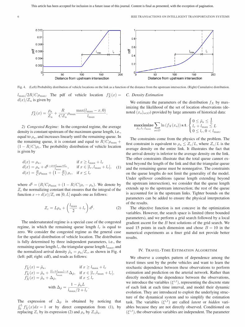
Fig. 4. (Left) Probability distribution of vehicle locations on the link as a function of the distance from the upstream intersection. (Right) Cumulative distribution.

lmax/2R/Cρmax. The pdf of vehicle location fuX(x) =

d(x)/Zu is given by

fuX(x) =

ρaZu

+R

CZuρmax

max(lmax − x, 0)lmax

.

2) Congested Regime: In the congested regime, the averagedensity is constant upstream of the maximum queue length, i.e.,equal to ρa, and increases linearly until the remaining queue. Inthe remaining queue, it is constant and equal to R/Cρmax +(1 −R/C)ρc. The probability distribution of vehicle locationis given by

d(x) = ρa, if x ≥ lmax + lrd(x) = ρa + d� −x+lmax+lr

lmax, if x ∈ [lr, lmax + lr],

d(x) = RC ρmax +

(1 − R

C

)ρc, if x ≤ lr

(1)

where d� = (R/Cρmax + (1 −R/C)ρc − ρa). We denote byZc the normalizing constant that ensures that the integral of thefunction x → d(x)/Zc on [0, L] equals one as follows:

Zc = Lρa +

(lmax

2+ lr

)d�. (2)

The undersaturated regime is a special case of the congestedregime, in which the remaining queue length lr is equal tozero. We consider the congested regime as the general casefor the spatial distribution of vehicle location. The distributionis fully determined by three independent parameters, i.e., theremaining queue length lr, the triangular queue length lmax, andthe normalized arrival density ρa = ρa/Zc, as shown in Fig. 4(left: pdf; right: cdf), and reads as follows:

f cX(x) = ρa, if x ≥ lmax + lrf cX(x) = ρa +

(lr+lmax)−xlmax

Δρ, if x ∈ [lr, lmax + lr],f cX(x) = ρa +Δρ, if x ≤ lr

with Δρ =1 − ρaL

lmax/2 + lr.

The expression of Δρ is obtained by noticing that∫ L

0 f cX(x)dx = 1 or by direct computation from (1), by

replacing Zc by its expression (2) and ρa by Zcρa.

C. Density Estimation

We estimate the parameters of the distribution fX by max-imizing the likelihood of the set of location observations (de-noted (xo)o∈O) provided by large amounts of historical data:

maximizeρa,lr,lmax

∑o∈O

ln (fX(xo)) s.t.

⎧⎨⎩

0 ≤ ρa ≤ 1L

lr + lmax ≤ L0 ≤ lr, 0 < lmax.

The constraints come from the physics of the problem. Thefirst constraint is equivalent to ρa ≤ Zc/L, where Zc/L is theaverage density on the entire link. It illustrates the fact thatthe arrival density is inferior to the average density on the link.The other constraints illustrate that the total queue cannot ex-tend beyond the length of the link and that the triangular queueand the remaining queue must be nonnegative. The constraintson the queue lengths do not limit the generality of the model.Under spillover conditions (queue length extending beyondthe upstream intersection), we consider that the queue lengthextends up to the upstream intersection; the rest of the queueis accounted for in the upstream links. Tighter bounds on theparameters can be added to ensure the physical interpretationof the results.

The objective function is not concave in the optimizationvariables. However, the search space is limited (three boundedparameters), and we perform a grid search followed by a localgradient ascent for the B best solutions of the grid search. Weused 15 points in each dimension and chose B = 10 in thenumerical experiments as a finer grid did not provide betterresults.

IV. TRAVEL-TIME ESTIMATION ALGORITHM

We observe a complex pattern of dependence among thetravel times sent by the probe vehicles and want to learn thestochastic dependence between these observations to performestimation and prediction on the arterial network. Rather thandirectly modeling the dependence between the observations,we introduce the variables (ξi,t), representing the discrete stateof each link at each time interval, and model their dynamicevolution. They are introduced to exploit the underlying struc-ture of the dynamical system and to simplify the estimationtask. The variables (ξi,t) are called latent or hidden vari-ables because they are not directly observed. Conditioned on(ξi,t), the observation variables are independent. The parameter



estimation problem would be simplified if we could directlyobserve the state variables (ξi,t). Without observing (ξi,t),the likelihood function is a marginal probability, obtained bysumming (or integrating in the continuous case) over the latentvariables. Marginalization couples the parameters and obscuresthe underlying structure of the likelihood function. The EMalgorithm learns the dependence among the observations whileexploiting the structure of the stochastic dynamic evolution[14]. Given the parameters of the dynamics and the observationmodel, we can compute the probability distribution of the latentvariables. Similarly, given the probability distribution of thelatent variables, we can compute the parameters that best ex-plain the observed data. Section IV-A provides a mathematicaljustification for the use of this iterative algorithm. We detail thesteps of the algorithm, i.e., the E step in Section IV-B and theM step in Section IV-C in the case of traffic estimation.

A. Introduction on the EM Algorithm

The EM algorithm allows us to exploit the underlying struc-ture of the dynamical model, although the latent variables arenot observed. It is an iterative algorithm consisting in two steps.

• The E step computes the joint probability distribution ofthe latent variables given the observed variables and thecurrent values of the parameters. In the case of a DBN,this step corresponds to a smoothing step, in which, at eachtime t, we estimate the joint probability distribution of thestate variables (ξi,t)i,t. In practice, the smoothing step isreplaced by a filtering step for efficiency. The filtering steponly uses observations received up to (and including) timet to compute the joint probability distribution of the statevariables (ξi,t)i.

• The M step optimizes the parameters based on the esti-mation of the joint probability distribution of the latentvariables. This step has the same complexity as if the latentvariables were observed.

Let Y denote the observable RV, with realization y (traveltime from the probe vehicles) and ξ as the latent variables, withrealization s (congestion state of the links of the network). Letθ be the set of unknown parameters, i.e., θ = {(μi,s, σi,s), i ∈I, s ∈ {0, . . . , S − 1}} ∪ {Ai, i ∈ I}. The log likelihood of thedata is the log of the marginal probability of the observationsgiven the parameters, as given in

l(θ; y) = ln (p(y|θ)) = ln

(∑s

p(s, y|θ)).

If ξ was observed, the maximum likelihood estimation wouldamount to maximizing lc(θ; y, s) = ln(p(y, s|θ)), which is re-ferred to as the complete log likelihood, because it correspondsto the log probability of the complete set of RVs for a givenvalue of the parameter θ. Given that ξ is in fact not observed,the complete log likelihood is a random quantity and cannotbe directly maximized. Given a distribution, which is denotedas q(s|y), we define a deterministic function of θ, which isdenoted as 〈lc(θ; y, s)〉q and called the expected complete loglikelihood: It corresponds to the average of the complete log

likelihood, over the realizations of ξ, when q(s|y) is chosen asthe averaging distribution, i.e.,

〈lc(θ; y, s)〉q =∑s

q(s|y) ln (p(y, s|θ)) .

We use Jensen’s inequality and have

l(θ; y) ≥∑s

q(s|y) ln(p(s|y, θ)q(s|y)

)

=∑s

q(s|y) ln p(s, y|θ)−∑s

q(s|y) ln q(s|y).

To maximize l(θ; y), we iteratively maximize the right-handside by 1) maximizing on the proposal distribution q(s|y) giventhe current value of the parameter (E step) and 2) maximizingon the parameter θ given the proposal distribution (M step).

B. E Step

In the Bayesian approach to dynamic state estimation, oneattempts to construct the probability distribution of the state(belief state) at time interval t based on all available measure-ments up to and including time interval t, which is known asthe posterior distribution. The process of estimating the pdf ofthe state of the network at time interval t conditioned on theobservations up to time t is called filtering. The E step of theEM algorithm technically requires smoothing, i.e., estimatingthe pdf of the state conditioned on all the observations avail-able for the experiment. However, the smoothing is typicallyreplaced by a filtering step for efficiency. Filtering consists ofessentially two stages: prediction and update. The predictionuses the transition probabilities to compute the belief state fromone measurement to the next. The update operation uses thelatest available measurements to modify the state probabilitydistribution using the Bayes rule.

The DBN used in this paper is a multiply connected beliefnetwork (at least one pair of variables has more than oneundirected path connecting them), in which probabilistic infer-ence is NP-hard [10]. In such networks, algorithms performingprobabilistic inference have a time complexity that, in the worstcase, is exponential in the number of hidden variables in thenetwork. We need approximation algorithms to perform prob-abilistic inference. Algorithms such as Monte Carlo simulation[41], variational methods [31], and belief state simplification[7] are commonly used to approximate probabilistic inference.We investigate a Monte Carlo simulation approach (particlefilter) described in the following.

Particle filtering is an approximation of a recursive Bayesianfilter algorithm using Monte Carlo simulations, which hassuccessfully been implemented for highway traffic estimation[9]. The belief state is represented by a set of random sampleswith associated weights (importance weights) such that, as thenumber of samples increases, the approximation tends to thetrue belief state. We simulate V particles (V = 2000 inthe numerical experiments). Each particle v represents an in-stantiation of the time evolution of the traffic state of thenetwork, i.e., a possible succession of traffic states for each



link and each time interval. A particle v at time t is repre-sented by a vector of the states of each link and each timeinterval (si,t

′v )i∈I,t′∈{0...t}. At t, each particle has a weight ωt

v

proportional to the probability of having this instantiation of thestate evolution given the available data up to time t. The parti-cles explore the possible state space and represent the beliefstate of the DBN. At time t, the spatiotemporal instantiationsstv = (si,t

′v )i∈I, t′∈{0...t} of the particles and their associated

importance weight ωtv form an approximation pV (s

1:t|y1:t, θ)of the joint probability distribution p(s1:t|y1:t, θ) of the stateof the links up to time t. According to this approximation, theprobability of observing a state s = (si,t)i∈I, t∈{0...T } on thenetwork throughout its time evolution is

p(s|y, θ) ≈ pV (s|y, θ)

=

V∑v=1

ωTv 1s(sv)

where 1s(sv) is equal to 1 if the particle has the state instantia-tion s and 0 if otherwise. In particular, we define the followingsufficient statistics (SS):

• The path SS is the joint distribution of the states ofthe links j(k), on path k, conditioned on the obser-vations received up to time interval t. It is denotedas pV (s

j(k),t|y1:t, θ) and is computed by summing theweights of all the particles for which the links j(k) arein state sj(k),t ∈ S |j(k)| at t:

pV (sj(k),t|y1:t, θ) =

V∑v=1

ωv1sj(k),t

(sj(k),tv

).

• The link SS is the probability of the state of link i attime t, conditioned on the state of the neighbors πi attime interval t− 1 and the observations received up to t.It is denoted as pV (s

i,t|sπi,t−1, y1:t, θ) and is computedby summing the weights of all the particles for which linki is in state si,t ∈ S at t and for which the neighbors oflink i are in state sπi,t−1 ∈ S |πi| at t− 1. To compute theconditional probability, this sum is normalized by the sumof the weights of the particles for which the neighbors oflink i are in state sπi,t−1.

For each link and each time interval, the number of SS tocompute is exponential in the number of neighbors of the link.We present a model that overcomes this computational costby assuming that the state of a link at time t depends on thetotal number of undersaturated neighbors at t− 1, defined byηi,t−1 =

∑i′∈πi

si′,t−1. The number of SS to compute for link

i is |πi|+ 1 for each time interval, which significantly limitsthe complexity. Other functions could be used to compactlyrepresent the state of the neighbors. We experiment with a fewother choices in the numerical experiments. These functionsdo not need to be linear nor 1-D. The SS pV (s

i,t|ηi,t−1, y, θ)are similarly computed as for pV (s

i,t|sπi,t−1, y, θ): We sumthe weights of the particles for which link i is in state si,t

at time interval t and for which the sum of the congestion of

the neighbors is ηi,t−1 at time interval t− 1 and normalize asfollows:

pV (si,t|ηi,t−1, y1:t, θ) =

V∑v=1

ωtv1si,t,ηi,t−1

(si,tv , ηi,t−1

v

)Z(ηi,t−1)

.

The constant Z(ηi,t−1) = pV (ηi,t−1|y1:t, θ) is computed from

the particles or, with less computational cost, by summing thejoint probabilities pV (s

i,t, ηi,t−1) over the possible states oflink i at time t.

Using these SS, the expected complete log likelihood〈lc(θ; y, s)〉pV

is given by∑t∈T \{0}si,t∈S

∑ηi,t−1

pV (si,t|ηi,t−1, y1:t, θ) ln

(A(ηi,t−1, si,t)

)

+∑t∈T

k∈K(t)

∑sj(k),t

pV (sj(k),t|y1:t, θ) ln f(yk|sj(k),tθ)

where sj(k),t ∈ {0, . . . , S − 1}|j(k)|, ηi,t−1 ∈ {0, . . . , |πi|},K(t) is the set of paths from probe vehicles received duringtime interval t, and f(yk|sj(k),t, θ) is the density of probabilityof the travel time yk on the links of the path j(k) that are in statesj(k),t. The mean and variance of travel times are computed bysumming the mean and variance travel times of the (partial)links of the path. We recall that the mean and variance of traveltimes on partial link i are scaled according to the function αi.In the first sum, we remove 0 from the set T since there is notransition prior to t0. To compute the SS, the filtering step isperformed with the particles as follows:

• Update at t: Compute the posterior distribution using themeasurements of time interval t. For each particle, ωt

v ismultiplied by the probability of each measurement giventhe states ξi,tv of the particle. The weights are normalizedso that they sum to 1.

• Prediction at t+ 1: Predict the state distribution for timeinterval t+ 1 using the transition probabilities. For eachlink i and each particle v, we sample the state ξi,t+1

v giventhe states ξπi,t

v (or any function of the states such as thesum of the congestion states) of its neighbors at timet according to the transition probabilities, i.e., the statesi,t+1 is chosen with probability A(si,t+1|ξπi,t

v ).

This algorithm is known as a sequential importance sampling(SIS) particle filter [2]. A common problem with the SIS parti-cle filter is the degeneracy phenomenon [15], [17]. After a fewiterations, all but one particle have negligible weights. A largecomputational effort is devoted to updating particles whosecontribution to the posterior distribution is almost zero. Toreduce the effects of degeneracy, we resample the particles afterthe update step. The modified algorithm is known as sequentialimportance resampling or sampling importance resampling.To resample the particles, V particles are successively chosenrandomly (with replacement) with a probability equal to itsweight (the weights sum to 1). The new set of particles allhave a weight equal to 1/V and is used to compute the a prioriprobability distribution of the states at time interval t+ 1.



Fig. 5. Resampling algorithm: Each particle is represented by a circle with a diameter proportional to its weight. Each particle is chosen with a probabilityproportional to its weight, put in the new set of particles with weight 1/V , and then replaced. This process is repeated V times. The intuition is that particles witha large weight are likely to be chosen several times, whereas particles with a small weight might not be present after the resampling step.

C. M Step: Update of the Model Parameters

The M step maximizes the expected complete log likelihoodwith respect to θ, representing the parameters of both thedynamics (transition probability matrices Ai, i ∈ I) and theobservations (parameters of the travel-time distributions, whichare conditioned on the state of the link). Given the structure ofthe complete log likelihood, this optimization can be indepen-dently performed for each transition probability matrix Ai andfor the parameters of the joint Gaussian distribution. Note thatbecause travel-time observations may span several links, theestimation of the travel-time distribution couples all the linksof the network.

• The transition probability matrices are updated by max-imizing with respect to the entries of Ai under the con-straint that Ai is a stochastic matrix (all the lines havenonnegative entries and sum to 1). For the line j repre-senting the transition probability when the neighbors arein state m ∈ {0, . . . , S − 1}|πi|, we have

Ai(m, s) ∝∑

t∈T \{0}

pV (si,t = s|sπi,t−1 = m, y1:t, θ)

where the proportionality constant is computed for allm such that

∑s A

i(m, s) = 1. A similar expression isobtained if the transitions depend on any functions of thestates, such as the number of undersaturated neighbors.

• Given the discrete state of link i at time interval t, thetravel time on link i, i.e., Y i,t, is normally distributed.Remember that the pdf of a partial travel time is com-puted from the pdf of a link travel time using the scal-ing function αi(·, ·) shown in Section III, although thedependence does not explicitly appear for notational sim-plicity. The travel times are independent RV: Given thestate s of the network at time t, Y I,t is a multivariateGaussian variable with mean μs = (μi,si i ∈ I) and co-variance Σs = diag((σi,si)2 : i ∈ I), where si is the ithcoordinate of s and represents the state of link i. TheM step updates the mean μ = (μi,s i ∈ I, s ∈ {0, . . . ,S − 1}). We also use the notation Σ = diag((σi,s)2 : i ∈I, s ∈ {0, . . . , S − 1}). It is the solution of the followingoptimization problem:

minimizeμ∈R|S|×|I|

∑k t∈T

k∈K(t)

∑sj(k),t

pV (sj(k),t|y, θ)

×(yk − μsj(k),t

)T (Σsj(k),t

)−1(yk − μsj(k),t

).

Given that Σsj(k),tis positive definite for all k, the objective

function is convex in μ. However, the objective function is notjointly convex in μ and Σ, and we only optimize on μ; thevariances are estimated once at the beginning of the algorithmusing a Gaussian mixture with two components. The numberof variables grows linearly with the number of links. We addconstraints to limit the feasible set to physically relevant valuesand implement an interior point algorithm [6].

Algorithm 1 Maximum likelihood estimation of the param-eters of the dynamic and observation models.

Initialize the parameters: (μi,s, σi,s)i,s, (Ai)i.EM algorithm for parameter estimation in DBNwhile The algorithm has not converged do

E Step (Section IV-B)Initialize the E Step: Simulate samples with weightωv = 1/V representing the state of the networkat the initial time given the initial state probabilities.for t ∈ T do

Update: For each travel-time observation, multiplythe weight of each particle with the probabilityof the observation given the state of the particle:ωv ← ωv

∏k fYk

(yk|ξj(k),tv )Normalize: divide the weight of each particle by thesum of the weights.Resample the particles to avoid degeneracy (seeFig. 5 and details in [2], [33]).Predict: For each link i and each particle v, samplethe state at time interval t+ 1 using the transitionprobabilities Ai.

end forM Step (Section IV-C)Update the transition probabilities Ai, i ∈ I .Update the parameters of the observation model.

end while

V. EXPERIMENTS

The model formalizes an intuitive representation of thepropagation of congestion throughout the network. This paperproposes a learning algorithm of the dynamics of traffic on anetwork and a real-time estimation framework. Our numericalresults are organized as follows. First, we validate the use ofthe model shown in Section III, which is denoted as the density



Fig. 6. Subnetwork of San Francisco used for validation.

model, to derive temporal averages of the probability distribu-tion of vehicle locations and use it for scaling partial traveltime. Second, we validate the DBN presented in this paper.Using cross-validation, we test the estimation and predictionaccuracy of the model for different time horizons. We compareour results to a baseline model and investigate how the use ofthe density model improves the results. We also validate thepdf of travel times learned by the model. The estimation ofthe travel-time distribution (rather than mean values only) iscrucial in arterial networks to accurately describe the variabilityof travel times.

A. Validation of the Density Model

Experimental setup: We use data collected by one of thefeeds of the Mobile Millennium system: a fleet of 500 vehiclesreporting their location every minute in San Francisco, CA.This paper focuses on a subnetwork of San Francisco (seeFig. 6) with 815 links and 527 intersections (more than 12.6 kmof roadway). A historical interval is a tuple consisting of a dayof the week, a start time, and an end time. For each historicalinterval and each link, we aggregate the locations reported bythe vehicles and learn the parameters of the density model.We focus our numerical results on 15-min intervals represent-ing Tuesdays from 4 P.M. to 8 P.M., i.e., (Tuesday, 4 P.M.,4:15 P.M.), . . ., (Tuesday, 7:45 P.M., 8 P.M.).

Description of the statistical test of the model:For each link and each historical interval, we use theKolmogorov–Smirnov (K–S) statistics to test if the locationsof the probe vehicles are distributed according to the densitymodel [39]. The K–S statistic is computed as the maximumdifference between the empirical and the hypothetical cdf(density model). In contrast with other tests (e.g., T-test thattests uniquely the mean or the chi-squared test that assumesthat the data is normally distributed), the K–S test is a standardnonparametric test to state whether samples are distributedaccording to a hypothetical distribution. We use this test toaccept (or reject) the null hypothesis H0: “The measurements

TABLE IOUTCOME OF STATISTICAL TESTS

TABLE IIPERCENTAGE OF POSITIVE K–S TESTS FOR DIFFERENT VALUES OF α

AND THE TWO HYPOTHESIS (DENSITY MODEL OR

UNIFORM DISTRIBUTION)

of probe vehicles are distributed according to the densitymodel.” When performing a statistical test, four situationsdescribed in Table I arise. The performance of a statistical testis defined by its statistical significance (1 − α, where α is theprobability to reject H0 when it is actually true) and statisticalpower (1 − β, where β is the probability to accept H0 whenit is actually false). The p-value is used to decide if we acceptor reject the null hypothesis H0. Low p-values indicate thatthe data do not follow the proposed distribution. We rejecthypothesis H0 at the α significance level if the p-value issmaller than α and accept it otherwise. The parameter α iscommonly set to values ranging from 0.001 to 0.1 and oftenset to α = 0.05. Smaller levels of α increase confidence in thedetermination of significance but increase the risk of Type IIerrors, and therefore have less statistical power. The K–Stest has a probability of Type II error β that tends to zero asthe number of samples tends to infinity. Since the number ofsamples is finite, we maintain the power of the statistical testby 1) not testing links that do not have enough measurements,2) experimenting with different levels of significance, and3) reporting the p-value for each decision.

We want to validate the capability of the density modelto properly scale travel time on portions of arterial links. Inparticular, we want to show that vehicles are not uniformly dis-tributed along the link since they are more likely to experiencedelay close to the downstream intersection. To illustrate thisreasoning, we also perform the K–S test with a null hypothesisbeing that measurements are uniformly distributed along thelink. We compare the results of the test on both hypothesesin Table II.

The results indicate that, for a majority of arterial links, theaverage location of vehicles is an RV that follows the densitymodel. The spatial distribution of vehicle location is betterrepresented by the density model than by a uniform distribu-tion. A graphical representation of the data provides valuablequalitative information: For different links of the network, werepresent the cumulative locations reported by the vehicles.2 We

2The cumulative locations are computed as follows: 1) We order the locationsreported by the probe vehicles; and 2) we plot the points (xi, i/N) for i =1 . . . N , where N is the number of locations collected for the link and historicinterval, and xi is the ith location on the link (in meters from the upstreamintersection).



Fig. 7. Empirical and proposal cdf of the average vehicle locations. (Top)Link with a p-value equal to 0.09. The model predicts a sharp increase in thedensity of measurements toward the downstream extremity of the link, but nomeasurements are received on the last 15 m of the link. The digital map does notmodel the width of the road or the intersection, which might explain the absenceof measurements on the last 15 m. (Bottom) Link with p-value equal to 0.33.The model learns the characteristics of the distribution of vehicle locations.We read an estimate of the historical queue length (around 30 m) that providesinformation on the average congestion of the link.

Fig. 8. Detecting signal locations using the average spatial distribution ofvehicles. The figure show an example of a very low p-value for a link of thenetwork. Analyzing the results, we realized that a signal was missing in thedatabase, explaining the poor fit of the model.

also represent the empirical (Kaplan–Meier) cdf [32] and theproposed cdf. In Fig. 7, we show the cumulative distributionsobtained for two links of the network during the first historicalinterval. The first link shows a good qualitative fit. However,the p-value is only 0.091. The map discretization does not takeinto account the width of intersections and may be the reasonwhy no measurements are received on the last 15 m of thelink. The second link has an average p-value. In both cases, thedata follows the sharp increase in the density of measurementsclose to the downstream intersection, as predicted by the modelbecause of the presence of a traffic signal. The model alsoprovides an estimate of the historical queue length on eachlink of the network that can be used for planning and networkcongestion analysis.

The analysis of the links with low p-values is also informativeand valuable. Fig. 8 shows the result for a link with a p-valueequal to 6.8 × 10−4. We expect sharp increases in the densityof measurements to occur upstream of traffic signals. The mapdatabase, provided to us by NAVTEQ, contains attributes of thetransportation network, such as road characteristics, presence oftraffic lights, and so on. On this link, the cumulative distributionof vehicle location exhibits two important increases, whereasonly one signal was present in the map database.

Analyzing the location of the link in Google Street View, weconfirmed that there was a signal that was not in the database.With the corrected information, we updated the proposed dis-

tribution and obtained a p-value equal to 0.29. A potentialapplication of the algorithm is the automatic detection of trafficsignals from probe data [24] but is not developed in this paper.Other sources of poor fitting are due to specific behaviors ofthe taxi, such as waiting in front of major hotels, which can befiltered, when considering successive locations of a taxi.

B. Validation of the Dynamic Bayesian Modeling

As probe vehicles report their location periodically in time,the duration between two successive location reports xs andxe represents an observation of the travel time of the vehicleon its path from xs to xe, i.e., the realizations yk of the RVsYk. A map-matching and path-inference algorithm [30] thatcombines models of GPS emissions and of drivers’ behaviorinto a conditional random field, filters out GPS noise, maps theGPS measurements to the road network, and reconstructs themost likely set of links traversed by the vehicle.

In our case study, we focus on learning the model parameterson Tuesdays from 4 P.M. to 8 P.M. in the subnetwork ofSan Francisco depicted in Fig. 6. We use 5 min as the timediscretization Δ in the graphical model shown in Section II.We assume that, conditioned on the state of the links of thenetwork, the travel times are independent Gaussian variables.The choice of a Gaussian distribution may restrict the flexibilityof the model to capture unique traffic characteristics, but it ismore computationally efficient in practice. In particular, themodel relies on travel times from probe vehicles that typicallytraverse several links between successive observations. Thetravel time on the path is a sum of independent RVs, and its pdfis computed as the convolution of the pdf of the link travel timeson the path. If the link travel times are normally distributed, thecomputation of the convolution is straightforward, whereas itrequires numerical algorithms, if otherwise. Finding tractableapproximation methods for using traffic-theory-inspired travel-time distributions is the subject of ongoing work [26]. We usethe density model to compute the pdf of partial link travel timesfrom the pdf of link travel times.

To validate the use of the DBN, we assess the estimationand prediction accuracy of the model. In traffic estimation (orprediction), access to ground-truth data is rare as it requiresthe monitoring of each vehicle on the entire network for theduration of the estimation. Instead, cross-validation [34] iscommonly used in the machine learning community to assesshow the results of a statistical model generalize to an inde-pendent data set, which is not used to develop the model butassumed to follow the same model. For each time interval,we randomly partition the available data (travel-time measure-ments of the probe vehicles) into complementary subsets. Welearn the parameter of the model on one subset (training set)and validate the performance of the model on the other subset(validation or testing set). The training set constitutes 70% ofthe available data, and the remaining 30% is used for validation.

Estimation and prediction errors: We compare the traveltimes predicted by the model with the travel times reported bythe probe vehicles and compute the average l1 error. Given aset of observations yk, k ∈ K(t) received at time interval t andcorresponding estimates (predictions) yk, the average lp error



Fig. 9. Evolution of the estimation and prediction of the percentage l1 erroron the validation data set.

ep is given by ep = (∑K(t)

k=1 |yk − yk|p/|Y|)1/p. The error istypically normalized by the average travel-time measurementsy (time between successive measurements), and we reportthe percentage of error ep = ep/y. Without a reference, thesevalues are hard to interpret: Travel times on arterial networkshave a high variance due to, in particular, the presence of trafficsignals [27]. Under similar traffic conditions, the travel times ofvehicles on an arterial link significantly vary depending on thetime at which the vehicle entered the link and the correspondingwaiting time at the signal. To improve interpretability of theresults of the model, we compare it to a baseline model: a time-series model adapted to probe vehicle data. If probe vehiclessent their travel times between defined positions, time seriescould be applied to estimate the travel time between thesepositions. However, no two distinct vehicles report their traveltime between the same locations. We propose a baseline modelthat adapts the traditional time series approach to probe-vehicledata. Travel times are decomposed onto the links of the path,and partial link travel times are scaled onto link travel times.We then use a moving average estimation. We also validate theuse of the density model to compute partial link travel times bycomparing the errors of the DBN model with and without thedensity model (scaling of partial link travel times using thefraction of the link traversed). To study the importance ofthe DBN structure, we consider a model, which is denoted asself only, with no spatial dependence: In the 2TBN, the edgesrepresenting the dynamics only connect the same links. Toshow the generality of the spatial dependence allowed by theframework, we consider a model, which is denoted as not self,where we remove same link edges from time intervals t to t+ 1in the 2TBN in Fig. 2.

Fig. 9 compares the results of the proposed model (estimationand 15-min forecast capabilities) with the baseline model. Wenotice a significant improvement in the percentage of errorcompared with the baseline model. The prediction decreaseswith the horizon of prediction but remains better than thebaseline. Note that the baseline model does not have predictioncapabilities.

Table III compares the results of the DBN with or withoutthe density model and validates the use of the density modelingto scale partial travel times and compute the pdf of traveltimes on partial links. The results also validate the short-termprediction capabilities of the DBN (both with and without thedensity modeling) and underline the importance of the richDBN structure, as shown by the better results of the modelcompared with simpler DBN structures (not self and self only).

TABLE IIIPERCENTAGE OF l1 ERROR OF THE MODEL COMPUTED ON A VALIDATION

DATA SET TO TEST THE ESTIMATION AND PREDICTION

CAPABILITIES OF THE MODEL

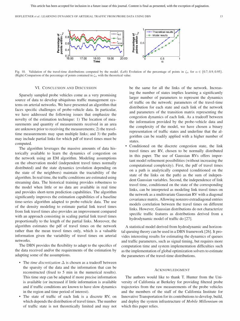
Validation of the estimated travel-time distributions: Thealgorithm produces more information than a single mean traveltime: 1) It characterizes the pdf of travel times on the net-work; 2) it estimates the probability of congestion pi,t of eachlink i and time interval t; and 3) it provides the parametersof the Gaussian distributions (μs,i, σs,i). The distribution oftravel times on any path j(k) can be sampled and numericallyapproximated using algorithm 2. We use 1000 samples in thefollowing. We define ζα as ζα = {y ∈ R : P(yk ≤ y) = 1 −α/2,P(yk ≥ y) = (1 + α)/2}. The probability that yk is ininterval ζα is α. For a Gaussian distribution, ζ0.68 (resp. ζ0.95)is the interval centered around the median of length two (resp.four) standard deviations. If the estimation of the travel-timedistribution is exact, the percentage of points in ζα is equal toα. The comparison of the percentage of points in ζα with αassesses the goodness of fit of the travel-time distributions withthe testing data (see Fig. 10).

Algorithm 2 Travel-time sampling

yk = 0 % Initialize the path travel-time samplefor l = 1 : j(k) do

r = rand(); % Choose the congestion stateif r < pc,l theng = μ0,l + σ0,lrandn()yk = yk + g % Add the sampled link travel timeto the path travel time

elseg = μ1,l + σ1,lrandn()yk = yk + g % Add the sampled link travel timeto the path travel time

end ifend for

We study the evolution of the percentage of points in ζα fordifferent values of α over the validation period. The percentageof points in ζα varies over time but remains close to its theoret-ical value (α), as shown on the left side of Fig. 10. On the rightof Fig. 10, we represent the percentage of points in ζα (averagedon the entire validation period) as a function of α. For all valuesof α, the percentage of points in ζα is slightly inferior to α. Thedifference between the theoretical and result curves is mostlydue to small inaccuracies in the estimation of the mean and/orunderestimation of the variance of the distribution. Note that ifthe curve produced by the model (dashed line with circles) wasover the theoretical line, it would indicate an overestimation ofthe variance.



Fig. 10. Validation of the travel-time distributions computed by the model. (Left) Evolution of the percentage of points in ζα for α ∈ {0.7, 0.9, 0.95}.(Right) Comparison of the percentage of points contained in ζα with the theoretical value.

VI. CONCLUSION AND DISCUSSION

Sparsely sampled probe vehicles come as a very promisingsource of data to develop ubiquitous traffic management sys-tems on arterial networks. We have presented an algorithm thatfaces specific challenges of probe-vehicle data. In particular,we have addressed the following issues that emphasize thenovelty of the estimation technique: 1) The location of mea-surements and quantity of measurements received in an areaare unknown prior to receiving the measurements; 2) the travel-time measurements may span multiple links; and 3) the pathsmay include partial links for which pdf of travel times must becomputed.

The algorithm leverages the massive amounts of data his-torically available to learn the dynamics of congestion onthe network using an EM algorithm. Modeling assumptionson the observation model (independent travel times normallydistributed) and the state dynamics (evolution depending onthe state of the neighbors) maintain the tractability of thealgorithm. In real time, the traffic conditions are estimated usingstreaming data. The historical training provides robustness tothe model when little or no data are available in real timeand provides short-term prediction capabilities. The algorithmsignificantly improves the estimation capabilities of a baselinetime-series algorithm adapted to probe-vehicle data. The useof the density modeling to estimate partial link travel timesfrom link travel times also provides an improvement comparedwith an approach consisting in scaling partial link travel timesproportionally to the length of the partial links. Moreover, thealgorithm estimates the pdf of travel times on the networkrather than the mean travel times only, which is a valuableinformation given the variability of travel times on arterialnetworks.

The DBN provides the flexibility to adapt to the specifics ofthe data received and/or the requirements of the estimation byadapting some of the assumptions.

• The time discretization Δ is chosen as a tradeoff betweenthe sparsity of the data and the information that can bereconstructed (fixed to 5 min in the numerical results).This time step can be adapted if more precise informationis available (or increased if little information is availableand if traffic conditions are known to have slow dynamicsin the region and time period of interest).

• The state of traffic of each link is a discrete RV, onwhich depends the distribution of travel times. The numberof traffic state is not theoretically limited and may not

be the same for all the links of the network. Increas-ing the number of states implies learning a significantlylarger number of parameters to represent the dynamicsof traffic on the network: parameters of the travel-timedistribution for each state and each link of the networkand parameters of the transition matrix representing thecongestion dynamics of each link. As a tradeoff betweenthe information provided by the probe-vehicle data andthe complexity of the model, we have chosen a binaryrepresentation of traffic states and underline that the al-gorithm can be readily applied with a higher number ofstates.

• Conditioned on the discrete congestion state, the linktravel times are RV, chosen to be normally distributedin this paper. The use of Gaussian RVs offers impor-tant model refinement possibilities (without increasing thecomputational complexity). First, the pdf of travel timeson a path is analytically computed (conditioned on thestate of the links on the path) as the sum of indepen-dent Gaussian variables. Second, the independence of linktravel time, conditioned on the state of the correspondinglinks, can be interpreted as modeling link travel times onthe network as a multivariate Gaussian RV with a diagonalcovariance matrix. Allowing nonzero extradiagonal entriesmodels correlation between the travel times on differentlinks. However, Gaussian distributions do not characterizespecific traffic features as distributions derived from ahydrodynamic model of traffic do [27].

A statistical model derived from hydrodynamic and horizon-tal queuing theory can be used in a DBN framework [26]. It pro-vides interesting results for estimating the dynamics of queuesand traffic parameters, such as signal timing, but requires morecomputation time and system implementation difficulties suchas the implementation of global optimization solvers to estimatethe parameters of the travel-time distributions.

ACKNOWLEDGMENT

The authors would like to thank T. Hunter from the Uni-versity of California at Berkeley for providing filtered probetrajectories from the raw measurements of the probe vehiclesand the members of the staff of the California Institute forInnovative Transportation for its contributions to develop, build,and deploy the system infrastructure of Mobile Millennium onwhich this paper relies.



REFERENCES

[1] Cabspotting. [Online]. Available: http://www.cabspotting.org[2] M. Arulampalam, S. Maskell, N. Gordon, and T. Clapp, “A tutorial on par-

ticle filters for online nonlinear/non-Gaussian Bayesian tracking,” IEEETrans. Signal. Proces., vol. 50, no. 2, pp. 174–188, Feb. 2002.

[3] X. Ban, R. Herring, P. Hao, and A. Bayen, “Delay pattern estimation forsignalized intersections using sampled travel times,” in Proc. 88th Transp.Res. Board Annu. Meeting, Washington, DC, Jan. 2009, pp. 109–119.

[4] A. Bayen, J. Butler, and A. Patire, “Mobile millennium final report,” Univ.California, Berkeley, CA, CCIT Res. Rep. UCB-ITS-CWP-2011-6, 2011.

[5] P. Bickel, C. Chen, J. Kwon, J. Rice, E. Van Zwet, and P. Varaiya, “Mea-suring traffic,” Stat. Sci., vol. 22, no. 4, pp. 581–597, 2007.

[6] S. P. Boyd and L. Vandenberghe, Convex Optimization. Cambridge,U.K.: Cambridge Univ. Press, 2004.

[7] X. Boyen and D. Koller, “Tractable inference for complex sto-chastic processes,” in Proc. 14th Conf. Uncertainty Artif. Intell., 1998,pp. 33–42.

[8] L. Chen, W. L. Jin, J. Hu, and Y. Zhang, “An urban intersection modelbased on multi-commodity kinematic wave theories,” in Proc. 11th IEEEIntell. Transp. Syst. Conf., 2008, pp. 269–274.

[9] P. Cheng, Z. Qiu, and B. Ran, “Particle filter based traffic state estimationusing cell phone network data,” in Proc. 9th Intell. Transp. Syst. Conf.,Sep. 2006, pp. 1047–1052.

[10] G. F. Cooper, “The computational complexity of probabilistic inferenceusing Bayesian belief networks,” Artif. Intell., vol. 42, no. 2/3, pp. 393–405, Mar. 1990.

[11] C. Daganzo, “The cell transmission model: A dynamic representation ofhighway traffic consistent with the hydrodynamic theory,” Transp. Res. B,vol. 28, no. 4, pp. 269–287, Aug. 1994.

[12] C. de Fabritiis, R. Ragona, and G. Valenti, “Traffic estimation and pre-diction based on real time floating car data,” in Proc. 11th IEEE Intell.Transp. Syst. Conf., 2008, pp. 197–203.

[13] T. Dean and K. Kanazawa, “A model for reasoning about persistence andcausation,” Comput. Intell., vol. 5, no. 3, pp. 142–150, Aug. 1990.

[14] A. P. Dempster, N. M. Laird, and D. B. Rubin, “Maximum likelihoodfrom incomplete data via the em algorithm,” J. Roy. Stat. Soc. Ser. B(Methodol.), vol. 39, no. 1, pp. 1–38, 1977.

[15] A. Doucet and N. de Freitas, Sequential Monte Carlo Methods in Practice.New York: Springer-Verlag, 2001.

[16] C. Furtlehner, J. Lasgouttes, and A. de la Fortelle, “A belief propagationapproach to traffic prediction using probe vehicles,” in Proc. 10th IEEEIntell. Transp. Syst. Conf., 2007, pp. 1022–1027.

[17] N. J. Gordon, D. J. Salmond, and A. F. M. Smith, “Novel approach tononlinear/non-Gaussian Bayesian state estimation,” Proc. Inst. Elect. Eng.F—Radar Signal Process., vol. 140, no. 2, pp. 107–113, Apr. 1993.

[18] I. Guyon and A. Elisseeff, “An introduction to variable and featureselection,” J. Mach. Learn. Res., vol. 3, pp. 1157–1182, Mar. 2003.

[19] B. Hellinga, P. Izadpanah, H. Takada, and L. Fu, “Decomposing traveltimes measured by probe-based traffic monitoring systems to individ-ual road segments,” Transp. Res. C, vol. 16, no. 6, pp. 768–782,Dec. 2008.

[20] R. Herring, “Real-time traffic modeling and estimation with streamingprobe data using machine learning,” Ph.D. dissertation, Univ. California,Berkeley, CA, 2010.

[21] R. Herring, A. Hofleitner, P. Abbeel, and A. Bayen, “Estimating arterialtraffic conditions using sparse probe data,” in Proc. 13th IEEE Intell.Transp. Syst. Conf., Madeira, Portugal, Sep. 2010, pp. 929–936.

[22] R. Herring, A. Hofleitner, S. Amin, T. Abou Nasr, A. A. Khalek,P. Abbeel, and A. Bayen, “Using mobile phones to forecast arterialtraffic through statistical learning,” presented at the 89th Transporta-tion Research Board Annual Meeting, Washington, DC, Jan. 2010,Paper 10-2493.

[23] A. Hofleitner and A. Bayen, “Optimal decomposition of travel timesmeasured by probe vehicles using a statistical traffic flow model,” in Proc.14th IEEE Intell. Transp. Syst. Conf., Oct. 2011, pp. 815–821.

[24] A. Hofleitner, E. Come, L. Oukhellou, J.-P. Lebacque, and A. Bayen,“Automatic signal detection leveraging sparsely sampled probe vehi-cles,” in Proc. 15th IEEE Intell. Transp. Syst. Conf., Anchorage, AK,Sep. 2012.

[25] A. Hofleitner, R. Herring, and A. Bayen, “A hydrodynamic theory basedstatistical model of arterial traffic,” Univ. California, Berkeley, CA, Tech.Rep. UCB-ITS-CWP-2011-2, Jan. 2011.

[26] A. Hofleitner, R. Herring, and A. Bayen, “Arterial travel timeforecast with streaming data: A hybrid flow model—Machinelearning approach,” Transp. Res. B, 2012, doi: 10.1016/j.trb.2012.03.006,to be published.

[27] A. Hofleitner, R. Herring, and A. Bayen, “Probability distributions oftravel times on arterial networks: A traffic flow and horizontal queuingtheory approach,” presented at the 91st Transp. Res. Board Annu. Meet-ing, Washington, DC, Jan. 2012, Paper 12-0798.

[28] E. Horvitz, J. Apacible, R. Sarin, and L. Liao, “Prediction, expectation,and surprise: Methods, designs, and study of a deployed traffic forecastingservice,” in Proc. 21st Conf. Uncertainty Artif. Intell., Edinburgh, U.K.,2005.

[29] B. Hull, V. Bychkovsky, Y. Zhang, K. Chen, M. Goraczko, A. Miu,E. Shih, H. Balakrishnan, and S. Madden, “CarTel: A distributed mobilesensor computing system,” in Proc. 4th Int. Conf. Embedded Netw. Sens.Syst., 2006, pp. 125–138.

[30] T. Hunter, T. Moldovan, M. Zaharia, S. Merzgui, J. Ma, J. Franklin,P. Abbeel, and M. J. Bayen, “Scaling the mobile millennium system inthe cloud,” in Proc. 2nd ACM SOCC, 2011, vol. 28, pp. 1–8.

[31] M. I. Jordan, Z. Ghahramani, T. S Jaakkola, and L. K. Saul, “An introduc-tion to variational methods for graphical models,” Mach. Learn., vol. 37,no. 2, pp. 183–233, Nov. 1999.

[32] E. L. Kaplan and P. Meier, “Nonparametric estimation from incompleteobservations,” J. Amer. Stat. Assoc., vol. 53, no. 282, pp. 457–481,Jun. 1958.

[33] G. Kitagawa, “Monte Carlo filter and smoother for non-Gaussian nonlin-ear state space models,” J. Comput. Graph. Stat., vol. 5, no. 1, pp. 1–25,Mar. 1996.

[34] R. Kohavi, “A study of cross-validation and bootstrap for accuracy esti-mation and model selection,” in Proc. 14th Joint Conf. Artif. Intell., 1995,pp. 1137–1143.

[35] A. Krause, E. Horvitz, A. Kansal, and F. Zhao, “Toward commu-nity sensing,” in Proc. 7th IEEE Conf. Inf. Process. Sens. Netw., 2008,pp. 481–492.

[36] J. Kwon and K. Murphy, “Modeling freeway traffic with coupledHMMS,” Univ. California, Berkeley, CA, Tech. Rep., 2000.

[37] J. P. Lebacque, “First-order macroscopic traffic flow models: Intersectionmodeling, network modeling,” in Proc. 16th Int. Symp. Transp. TrafficTheory, 2005, pp. 365–386.

[38] M. Lighthill and G. Whitham, “On kinematic waves. II. A theory of trafficflow on long crowded roads,” Proc. Roy. Soc. Lond. Ser. A, vol. 229,no. 1178, pp. 317–345, May 1955.

[39] F. J. Massey, “The Kolmogorov–Smirnov test for goodness of fit,” J. Amer.Stat. Assoc., vol. 46, no. 253, pp. 68–78, Mar. 1951.

[40] X. Min, J. Hu, Q. Chen, T. Zhang, and Y. Zhang, “Short-term traffic flowforecasting of urban network based on dynamic STARIMA model,” inProc. 12th IEEE Intell. Transp. Syst. Conf., 2009, pp. 1–6.

[41] R. M. Neal, “Probabilistic inference using Markov chain Monte Carlomethods,” Univ. Toronto. Dept. Comput. Sci., Toronto, ON, Canada, Tech.Rep. CRG-TR-93-1, 1993.

[42] T. Park and S. Lee, “A Bayesian approach for estimating link travel timeon urban arterial road network,” in Proc. Comput. Sci. Appl., May 2004,pp. 1017–1025.

[43] F. Porikli and L. Xiaokun, “Traffic congestion estimation using HMMmodels without vehicle tracking,” in Proc. IVS, Jun. 2004, pp. 188–193.

[44] A. Thiagarajan, L. Sivalingam, K. LaCurts, S. Toledo, J. Eriksson,S. Madden, and H. Balakrishnan, “VTrack: Accurate, energy-aware trafficdelay estimation using mobile phones,” in Proc. 7th Conf. EmbeddedNetw. Sens. Syst., Berkeley, CA, Nov. 2009, pp. 85–98.

[45] H. Van Zuylen, F. Zheng, and Y. Chen, “Using probe vehicle data fortraffic state estimation in signalized urban networks,” in Proc. Traffic DataCollect. Stand., 2010, pp. 109–127.

[46] D. B. Work, S. Blandin, O.-P. Tossavainen, B. Piccoli, and A. M. Bayen,“A traffic model for velocity data assimilation,” Appl. Math. Res. Exp.,vol. 2010, no. 1, pp. 1–35, Apr. 2010.

Aude Hofleitner received the Engineering degreein applied mathematics from Ecole Polytechnique,Palaiseau, France; the M.S. degree in transportationengineering from the University of Marne La Vallee,Marne La Vallee, France; and the M.S. degree inapplied mathematics from the Ecole Nationale desPonts et Chaussees, Paris, France. She is currentlyworking toward the Ph.D. degree in electrical engi-neering and computer science with the University ofCalifornia, Berkeley.

Ms. Hofleitner was a recipient of the Dwight DavidEisenhower Transportation Fellowship from the U.S. Department of Trans-portation and the Anita Borg Grace Hopper Conference Scholarship in 2011.

http://www.cabspotting.org



Ryan Herring received the Bachelor’s degree inapplied mathematics from Oberlin College, Oberlin,OH, in 2005 and the M.S. and Ph.D. degrees inindustrial engineering and operations research fromthe University of California, Berkeley, in 2006 and2010, respectively.

While he was a graduate student, he was withthe California Center for Innovative Transportation,University of California, Berkeley. He is currentlya Software Engineer with Apple, Inc. His researchinterests include big data, machine learning, and

estimation.

Pieter Abbeel received the B.S. and M.S. degreesin electrical engineering from Katholieke Univer-siteit Leuven, Leuven, Belgium, and the Ph.D. de-gree in computer science from Stanford University,Stanford, CA, in 2008.

Since 2008, he has been a Faculty Member withthe Department of Electrical Engineering and Com-puter Sciences, University of California, Berkeley.He has developed apprenticeship learning algo-rithms, which have enabled advanced helicopter aer-obatics, including maneuvers such as tic-tocs, chaos,

and autorotation, which only exceptional human pilots can perform. His grouphas also enabled the first end-to-end completion of reliably picking up acrumpled laundry article and folding it. His work has been featured in manypopular press outlets, including BBC, MIT Technology Review, DiscoveryChannel, SmartPlanet, and Wired.

Dr. Abbeel has received of various awards, including the Best Paper Awardsat the International Conference on Machine Learning and the InternationalConference on Robotics and Automation, the Sloan Fellowship, the OkawaFoundation Award, and 2011’s TR35.

Alexandre Bayen received the Engineering degreein applied mathematics from the Ecole Polytech-nique, Palaiseau, France, in 1998 and the M.S. andPh.D. degrees in aeronautics and astronautics fromStanford University, Stanford, CA, in 1999 and 2003,respectively.

From 2000 to 2003, he was a Visiting Researcherwith NASA Ames Research Center. He worked as aResearch Director with the Autonomous NavigationLaboratory, Laboratoire de Recherches Balistiques etAerodynamiques, Ministere de la Defense, Vernon,

France, where he holds the rank of Major. He is currently an Associate Pro-fessor with the Department of Electrical Engineering and Computer Sciences,University of California, Berkeley. He is the author of one book and over 100articles in peer-reviewed journals and conferences.

Dr. Bayen received the Ballhaus Award from Stanford University in 2004,the CAREER award from the National Science Foundation in 2009, and thePresidential Early Career Award for Scientists and Engineers in 2010. He isalso included in the NASA Top 10 Innovators on Water Sustainability in 2010.His projects Mobile Century and Mobile Millennium received the 2008 Bestof ITS Award for “Best Innovative Practice” at the ITS World Congress anda TRANNY Award from the California Transportation Foundation in 2009.Mobile Millennium has been featured more than 100 times in the media,including television channels and radio stations (CBS, NBC, ABC, CNET, NPR,KGO, and the BBC), and in the popular press (Wall Street Journal, WashingtonPost, and LA Times).

IEEETRANSACTIONS ON INTELLIGENT TRANSPORTATION SYSTEMS 1

Documents

Transcript of IEEETRANSACTIONS ON INTELLIGENT TRANSPORTATION SYSTEMS 1