IEEE/ACM TRANSACTIONS ON COMPUTATIONAL …users.cis.fiu.edu/~taoli/pub/feature-tcbb.pdf ·...

Feature Selection for Gene Expression UsingModel-Based Entropy

Shenghuo Zhu, Dingding Wang, Kai Yu, Tao Li, and Yihong Gong

Abstract—Gene expression data usually contain a large number of genes but a small number of samples. Feature selection for gene

expression data aims at finding a set of genes that best discriminate biological samples of different types. Using machine learning

techniques, traditional gene selection based on empirical mutual information suffers the data sparseness issue due to the small

number of samples. To overcome the sparseness issue, we propose a model-based approach to estimate the entropy of class

variables on the model, instead of on the data themselves. Here, we use multivariate normal distributions to fit the data, because

multivariate normal distributions have maximum entropy among all real-valued distributions with a specified mean and standard

deviation and are widely used to approximate various distributions. Given that the data follow a multivariate normal distribution,

since the conditional distribution of class variables given the selected features is a normal distribution, its entropy can be computed

with the log-determinant of its covariance matrix. Because of the large number of genes, the computation of all possible

log-determinants is not efficient. We propose several algorithms to largely reduce the computational cost. The experiments on

seven gene data sets and the comparison with other five approaches show the accuracy of the multivariate Gaussian generative model

for feature selection, and the efficiency of our algorithms.

Index Terms—Feature selection, multivariate Gaussian generative model, entropy.

Ç

1 INTRODUCTION

GENE expression refers to the level of production ofprotein molecules defined by a gene. Monitoring of

gene expression is one of the most fundamental approach ingenetics and molecular biology. The standard technique formeasuring gene expression is to measure the mRNAinstead of proteins, because mRNA sequences hybridizewith their complementary RNA or DNA sequences whilethis property lacks in proteins. The DNA arrays, pioneeredin [5] and [10], are novel technologies that are designed tomeasure gene expression of tens of thousands of genes in asingle experiment. The ability of measuring gene expressionfor a very large number of genes, covering the entiregenome for some small organisms, raises the issue ofcharacterizing cells in terms of gene expression, that is,using gene expression to determine the fate and functions ofthe cells. The most fundamental of the characterizationproblem is that of identifying a set of genes and itsexpression patterns that either characterize a certain cellstate or predict a certain cell state in the future [18].

When the expression data set contains multiple classes,the problem of classifying samples according to their geneexpression becomes much more challenging, especiallywhen the number of classes exceeds five [24]. Moreover,the special characteristics of expression data add more

challenge to the classification problem. Expression datausually contain a large number of genes (in thousands) anda small number of experiments (in dozens). In machinelearning terminology, these data sets are usually of veryhigh dimensions with undersized samples. In microarraydata analysis, many gene selection methods have beenproposed to reduce the data dimensionality [31].

Gene selection aims to find a set of genes that bestdiscriminate biological samples of different types. Theselected genes are “biomarkers,” and they form a “markerpanel” for analysis. Most gene selection schemes are basedon binary discrimination using rank-based schemes [8]such as information gain, which reduces the entropy of theclass variables given the selected features. One criticalissue in these rank-based methods is data sparseness. Forexample, the estimation of the traditional information gainis an empirical estimation directly on the data. Suppose weselect the 11th gene for a data set. The 10 selected genessplit the training data into 1;024 ¼ 210 groups (assumingthat each gene does a binary split). Since we have very fewsamples in most groups, the estimations of mutualinformation between the 11th gene and the target in eachgroup are not accurate. Thus, the information gain, whichis the sum of the mutual information over all groups, is notaccurate.

To overcome the issue of data sparseness, we propose amodel-based approach to estimate the entropy on themodel, instead of on the data themselves. Here, we usemultivariate Gaussian generative models, which model thedata with multivariate normal distributions. Multivariatenormal distributions are widely used in various areas,including gene expression data [34], because of theirgenerality and simplicity. The means of variables (expressiondata of genes and class labels) and the covariances betweenthem are two basic measures of variables themselves and

IEEE/ACM TRANSACTIONS ON COMPUTATIONAL BIOLOGY AND BIOINFORMATICS, VOL. 7, NO. 1, JANUARY-MARCH 2010 25

. S. Zhu, K. Yu, and Y. Gong are with NEC Laboratories America,10080 North Wolfe Road, Suite SW3-350, Cupertino, CA 95014.E-mail: {zsh, kyu, ygong}@sv.nec-labs.com.

. D. Wang and T. Li are with the School of Computer Science, FloridaInternational University, 11200 SW 8th Street, Miami, FL 33199.E-mail: {dwang003, taoli}@cs.fiu.edu.

Manuscript received 18 Oct. 2007; revised 17 Jan. 2008; accepted 13 Mar.2008; published online 10 Apr. 2008.For information on obtaining reprints of this article, please send e-mail to:[email protected], and reference IEEECS Log Number TCBB-2007-10-0136.Digital Object Identifier no. 10.1109/TCBB.2008.35.

1545-5963/10/$26.00 � 2010 IEEE Published by the IEEE CS, CI, and EMB Societies & the ACM

the interaction between them. To predict the classes of data,we have to model the interaction between genes and classlabels. Given the mean and covariance, multivariateGaussian is the distribution with the maximum entropy,which implies its generality according to the principle ofmaximum entropy [13]. Usually, we can explicitly andefficiently estimate parameters of multivariate Gaussianmodels via a few matrix operations, which implies thesimplicity of the models. Though the class variables arebinary or categorical, we relax them as numerical values,which bring us the simplicity. Our experiments suggest thatthis approximation in the feature selection does not affectthe classification accuracy.

A nice property of multivariate Gaussian distributionsis that the conditional distribution of a subset of variablesgiven another subset of variables is still a multivariateGaussian distribution. We can explicitly compute theentropy of class variables given the selected features withthe log-determinant of the covariance matrix of theconditional distribution [6], [3]. Therefore, the objectiveof minimizing the entropy becomes to find a set offeatures to minimize the log-determinant of the condi-tional covariance matrix. Because of the large number ofgenes, the computation of all log-determinants of theconditional covariance matrix is not time consuming. Wepropose several algorithms to largely reduce the computa-tional cost.

In summary, our contributions are the following:

1. We propose a model-based approach to estimate theentropy based on multivariate normal distributions.The model-based approach addresses the datasparseness problem in gene selection.

2. We propose several algorithms to efficientlycompute all log-determinants of the conditionalcovariance matrix and largely reduce the compu-tational cost. The assumption of multivariateGaussian generative models leads to simple,robust, and effective computation methods forgene selection.

3. We perform extensive experimental study on sevengene data sets and compare our algorithms withother five approaches.

The rest of the paper is organized as follows: A brief note onthe related work is given in Section 2. The notation used inthis paper is listed in Section 3. Our algorithms arepresented in Section 4, and the comparison methodologiesare described in Section 5. We show the experimentalresults in Section 6 and discuss the idea of experimentaldesigns and its connection with gene selection in Section 7.Finally, Section 8 concludes.

2 RELATED WORK

Generally two types of feature selection methods have beenstudied in the literature: filter methods [17] and wrappermethods [16]. Filter-type methods are essentially datapreprocessing or data filtering methods. Features areselected based on the intrinsic characteristics that determinetheir relevance or discriminative powers with regard to thetarget classes. In wrapper-type methods, feature selection is

“wrapped” around a learning method: the usefulness of afeature is directly judged by the estimated accuracy of thelearning method. Wrapper methods typically requireextensive computation to search for the best features. Aspointed out in [32], the essential differences between thetwo methods are

1. that a wrapper method makes use of the algorithmthat will be used to build the final classifier while afilter method does not, and

2. that a wrapper method uses cross validation tocompare the performance of the final classifier andsearches for an optimal subset while a filtermethod uses simple statistics computed from theempirical distribution to select an attribute subset.

Wrapper methods could perform better but would requiremuch more computational costs than filter methods. Mostgene selection schemes are based on binary discriminationusing rank-based filter methods [8] such as t-statistics andinformation gain [31]. One critical issue in these rank-basedmethods is data sparseness, and most of the rank-basedmethods do not take redundancy into consideration. Inorder to remove the redundancy among features, a Min-Redundancy and Max-Relevance (mRMR) framework isproposed in [25]. Yu and Liu [36] also explored therelationship between feature relevance and redundancyand proposed a method that can effectively removeredundant genes. In addition, ReliefF, a widely used featuresubset selection method, has also been applied to geneselection [22]. In the paper [19], a hierarchical Bayesianmodel is used to enforce the sparsity in the features.However, the sparsity is indirectly controlled by aparameter, not specified by the given number of featuresto select.

In Section 5, we will describe several gene selectionmethods used in our experimental comparisons in detail. Inthis paper, we propose a model-based approach to estimatethe information gain, instead of on the data itself. Thiswould overcome the limitations of data sparseness. Inaddition, the model parameters can be explicitly andefficiently estimated via a few matrix operations.

3 NOTATION

A summary of the notation we use in this paper is shown inTable 1.

4 MODEL-BASED FEATURE SELECTION

4.1 Feature Selection Using Entropy Measure

Suppose we have f feature variables of the underlying data,denoted by fXiji 2 Fg, where F is the full feature index set,having jF j ¼ f . We have the class variable, Y , represented bymultiple class indicator variables. For example, in a three-class classification problem, the class variables are repre-sented by vectors ð1;�1;�1Þ, ð�1; 1;�1Þ, and ð�1;�1; 1Þ.The problem of feature selection is to select a subset offeatures, S � F , to accurately predict the target Y , given thatthe cardinality of S ism ðm < fÞ. Let us denote fXiji 2 Sg byXS , for any set S.

26 IEEE/ACM TRANSACTIONS ON COMPUTATIONAL BIOLOGY AND BIOINFORMATICS, VOL. 7, NO. 1, JANUARY-MARCH 2010

The prediction capability of Y given XS can be measuredby the entropy of Y given XS , which is defined as

HðY jXSÞ ¼def �IEpðY ;XSÞ ln pðY jXSÞð Þ; ð1Þ

where IEpð�Þ is the expectation given the distribution p, andp stands for the underlying data distribution, i.e., the jointdistribution pðY ;XsÞ. The feature selection problem usingthe mutual information criterion is

arg minS

HðY jXSÞ: ð2Þ

Selecting an optimal subset of features is a combinatorialoptimization problem, which is an NP-problem. For theeffective practice is to take a greedy approach, i.e.,sequentially selecting features to achieve a suboptimalsolution. Given a selected feature set, S, the one-step goalof feature selection is to select one feature to minimize theentropy. The one-step objective, named as information gain,is to find i to maximize

IGði;SÞ ¼defHðY jXSÞ �H Y ;XS[fig

� �:

Then, the greedy procedure of feature selection based onmutual information is shown in Algorithm 1.

Algorithm 1. Feature selection by information gain

1: Let S ¼ ;;2: repeat

3: i ¼ arg maxi2F IGði;SÞ;4: S S [ fig;5: until jSj ¼ m.

The distribution pðY ;XSÞ can be estimated by theempirical distribution, i.e., measuring the proportion of Yand XS values in the given data. The empirical distributionfaces the data sparseness problem. Thus, we discuss the

estimation based on a multivariate Gaussian generative

model in the next section.

4.2 Multivariate Gaussian Model

We assume that the joint distribution of fXig and Y is a

multivariate normal (Gaussian) distribution:

z ¼ ½XFY � � N ð�;��;�Þ; ð3Þ

where �� is the mean vector, and � is the covariance matrix.

Let F be the index set of X in z and T be the index set of Y

in z. The reason is that the Gaussian assumption results in a

linear model, which is simple and scalable.We denote the feature values in the training data by eX,

where each row represents a sample, and each column

represents a feature (a gene). We consider multiple target

variables. For training data, we denote the target values aseY, where each row represents target variables of a sample,

and each column represents a target variable.Given the training data, we can estimate the parameters

of (3) by

b�� ¼def 1

n1>½eX; eY�; b� ¼def 1

nZ>Z; ð4Þ

where n is the number of rows of matrix eX, 1 is a column

vector of size n, whose elements are all ones, and

Z ¼def ½X;Y� ¼def ½eX; eY� � 1b��>: ð5Þ

Though the estimation of (4) is an unbiased estimation of

the covariance matrix, such estimation may suffer ill-posed

problems. By adding a regularization term, a robust

estimation can be obtained:

b� ¼ 1

nðZ>Zþ �IdÞ: ð6Þ

This is first proposed in [30]. Since (4) is a special case of (6),

we use (6) as the estimation of �.After the parameters of the model being estimated, we

do not differentiate the parameters and the estimated

parameters. For simplicity, we write b� by �. Since the

computation of the entropy does not involve ��, we let

�� ¼ 0 without loss of generality. Let z be a d-dimensional

vector, following the multivariate Gaussian distribution

Nðz; 0;�Þ. There are some properties of multivariate

Gaussian distribution.

Property 1. Let zS and zT be two subvectors of z, where S and T

are the index sets. We denote the subvector of �� corresponding

to an index set S by ��S and the submatrix of � corresponding

to index sets S and T by �ST . We have

PrðzT jzSÞ ¼def NðzT ;��T jS;�T jSÞ;

where

��T jS ¼def��T þ�TS��1

SSðzS � ��SÞ; ð7Þ

�T jS ¼def

�TT ��TS��1SS�ST : ð8Þ

This is the property of conditional distribution [26].

ZHU ET AL.: FEATURE SELECTION FOR GENE EXPRESSION USING MODEL-BASED ENTROPY 27

TABLE 1A Summary of Notation

Then, the property of the incremental updates is given asfollows:

Property 2. Let D be the full index set of z, S � F , i 2 F � S.

We have

�T jS[fig ¼ �ðSÞTT �

1

�ðSÞii

�ðSÞTi �

ðSÞiT ; ð9Þ

where

�ðSÞ ¼def��DS�

�1SS�SD: ð10Þ

Proof. Let T 0 ¼ T [ fig. By Property 1, PrðzT 0 jzSÞ follows a

Gaussian distribution with covariance �T 0 jS (see the

definition in (8)). By the definition of �ðSÞ, �T 0 jS is the

submatrix of �ðSÞ, whose column and row indices are T 0.

Since PrðzT jzS[figÞ ¼ PrðzT jzfig; zSÞ, applying Property 1

again, we obtain

�T jS[fig ¼ �ðSÞTT ��

ðSÞTi �

ðSÞii

h i�1�ðSÞiT :

As �ðSÞii is a scalar, we have (9). tu

The differential entropy of the multivariate normaldistribution can be computed by the following property.

Property 3.

HðzÞ ¼ �ZNðz;��;�Þ lnNðz;��;�Þdz

¼ 1

2ln j�j þ d

2lnð2�eÞ:

This can be found in [26].

Property 4.

HðY jXSÞ ¼1

2ln �T jS�� þ d

2lnð2�eÞ; ð11Þ

where T is its set of indices for Y in z.

By Properties 1 and 3, we have the property of theconditional multivariate normal distribution.

4.3 Feature Selection Algorithms

Now, we propose two sets of feature selection algorithmsbased on the multivariate Gaussian model and entropymeasure.

4.3.1 D-Optimality Feature Selection

In the multivariate Gaussian model, the problem of featureselection (2) becomes

arg minS

ln �T jS�� : ð12Þ

As the determinant of the covariance matrix is known asgeneralized variance. This criterion is to minimize thegeneralized variance of the joint distribution of targets.We name the feature selection based on the determinantcriterion (12) as the D-optimality Feature Selection after thedeterminant. We borrow the name of D-optimality fromexperimental designs [9].

As solving (12) is still an NP-problem, we use thegreedy approach as in Algorithm 1. Let �ðSÞ ¼ Kþ �Id. By(9), we have

ln �T jS[fig�� ¼ ln �

ðSÞTT �

1

�ðSÞii

�ðSÞTi �

ðSÞiT

� ��

¼ ln KTTþ�It�1

Kiiþ�ðKTiKiT Þ

�� ¼ lnjKTTþ�Itjþln 1�KiT ðKTTþ�ItÞ�1KTi

Kiiþ�

!;

ð13Þ

where t ¼ jT j. Therefore,

arg mini

ln �T jS[fig�� ¼ arg max

i

KiT ðKTT þ �ItÞ�1KTi

Kii þ �: ð14Þ

We can compute �ðS[figÞ from �ðSÞ by (10):

� S[figð Þ ¼�ðSÞ � 1

�ðSÞii

�ðSÞDi �

ðSÞiD

� �¼Kþ �Id �

1

Kii þ �KDiKiD þ ��iKiD þ �KDi��i

> þ �2��i��i>� �;

ð15Þ

where ��i is a column vector whose elements are zerosexcept that the ith element is one. Since we shall not select afeature twice, we shall no longer be concerned with thevalues in the ith row or column in K. Therefore, we canupdate K by K� 1

Kiiþ� ðKDiKiDÞ: By sequentially updatingK, we have Algorithm 2. Note that since we only comparethe values for features, we can drop the scale factor 1

n in (6)for simplicity. The complexity of Algorithm 2 isOðmðd2 þ dt2ÞÞ, where d ¼ jDj, and t ¼ jT j.

Since the complexity of the algorithm contains md2, the

algorithm is very inefficient when d is large. Especially,

the memory complexity is Oðd2Þ. When the sample size n

is much smaller than d, we can take advantage of it to

speed up the algorithm. Assume that K has the form of

Z>�Z. Note that � is symmetric since K is symmetric.

Initially, � ¼ In in step 2 of Algorithm 2.

Algorithm 2. D-Optimality feature selection I

1: S ¼ ;;2: K ¼ Z>Z;

3: repeat

4: Let U ¼ ðKTT þ �ItÞ�1;5: i ¼ arg max

i2F�SKiTUKTi

Kiiþ� ;

6: K K� 1Kiiþ� ðKDiKiDÞ;

7: S S [ fig;8: until jSj ¼ m.

Let us denote the ith column vector of X as xi. Theupdate of K can be written as

K� 1

Kiiþ�ðKDiKiDÞ¼Z>�Z� 1

xi>�xiþ�ðZ>�xixi

>�ZÞ:

ð16Þ

Therefore, we derive the update for � in Algorithm 3. Thecomplexity of the algorithm is Oðmðdn2 þ nt2 þ t3ÞÞ.


Algorithm 3. D-Optimality feature selection II1: S ¼ ;;2: � ¼ In;

3: repeat

4: Let � ¼ �YðY>�Yþ �ItÞ�1Y>�;

5: i ¼ arg maxi2F�S

xi>�xi

xi>�xiþ� ;

6: � �� 1xi>�xiþ� ð�xixi

>�Þ;7: S S [ fig;8: until jSj ¼ m.

N.B. xi is the ith column of centered feature matrix X.

When t < n, we can reduce the complexity by sequentiallycomputing �X ¼def

P. We have Algorithm 4, whose complex-ity is OðmdntÞ. Note that Phi and P in Algorithm 3 andAlgorithm 4 are used to save the intermediate results in the

matrix computation to reduce the computation complexity.

Algorithm 4. D-Optimality feature selection III

1: S ¼ ;;2: � ¼ In;

3: P ¼ X;4: repeat

5: Let R ¼ YððY>�Yþ �ItÞ�1Y>PÞ;6: i ¼ arg max

i2F�Sri>pi

xi>piþ� ;

7: � �� 1xi>piþ� ðpipi

>Þ;8: P P� 1

xi>piþ� ðpiðpi>XÞÞ;

9: S S [ fig;10: until jSj ¼ m.N.B. xi is the ith column of centered feature matrix X. pi is

the ith column of P, and ri is the ith column of R.

4.3.2 A-Optimality Feature Selection

Because of the complexity in computing determinants andthe nonconvexity of log-determinants, we can replace thelog-determinant of the covariance matrix with the trace of

the covariance matrix, which is the upper bound of the log-determinant of the covariance matrix.

Lemma 1. If X is a p� p positive definite matrix, it holds that

ln jXj � trðXÞ � p. The equality holds when X is an

orthonormal matrix.

Proof. Let f�1; � � � ; �pg be the eigenvalues of X. We have

ln jXj ¼P

i ln�i and trðXÞ ¼P

i �i. Since ln�i � �i � 1,we have the inequality. The equality holds when �i ¼ 1.Therefore, when X is an orthonormal matrix (especially

X ¼ Ip), the equality holds. tu

As ln j�T jSj � trð�T jSÞ � t, the problem of feature selec-tion (12) can be approximated by

arg minS

tr �T jS� �

¼ arg maxS

tr �TS��1SS�ST

� �: ð17Þ

Since the trace of the covariance divided by the number of

variables is the average covariance, (17) is calledA-optimality feature selection. We also borrow the name ofA-optimality from experimental designs, which is an

alternative of the D-optimality criterion [9].To sequentially solve (17), we have Algorithm 5. The

algorithm is similar to the sequential algorithm in [35],

which is to solve transductive active learning problems. Thecomplexity of Algorithm 5 is Oðmd2Þ.

Algorithm 5. A-Optimality feature selection I

1: S ¼ ;;2: K ¼ Z>Zþ �Id;

3: repeat


KiTKTi

Kiiþ� ;

5: K K� 1Kiiþ� ð�DiKiDÞ;


Whenn d, we can use a similar method as in Algorithm 3to speed up Algorithm 5. We can obtain Algorithm 5 by lettingU ¼ It in Algorithm 2. Then, we can use

� ¼ �YY>�

in step 4 of Algorithm 3 to obtain Algorithm 6. Thecomplexity of Algorithm 6 is Oðmdn2Þ.

Algorithm 6. A-Optimality feature selection II

1: S ¼ ;;2: � ¼ In;

3: repeat

4: Let � ¼ �YY>�;


xi>�xi

xi>�xiþ� ;

6: � �� 1xi>�xiþ� ð�xixi

>�Þ;7: S S [ fig;8: until jSj ¼ m.

N.B. xi is the ith column of centered feature matrix X.

We can also sequentially compute �X ¼defP as shown in

Algorithm 7, whose time complexity is Oðmdnþ dntÞ.

Algorithm 7. A-Optimality feature selection III

1: S ¼ ;;2: P ¼ X;3: R ¼ YðY>PÞ;4: repeat


ri>pi

xi>piþ� ;

6: R R� 1xi>piþ� ðriðpi

>XÞÞ;7: P P� 1

xi>piþ� ðpiðpi>XÞÞ;


N.B. xi is the ith column of centered feature matrix X. pi is

the ith column of P, and ri is the ith column of R.

Table 2 shows the summary of the complexity of theabove algorithms. In the gene expression data, which


TABLE 2The Complexity of Algorithms

The space complexity measures the extra required space besides data.

contain a large number of genes but a small number ofsamples, the D-opt III and A-opt III are the good choice forcomputational efficiency.

5 METHODS USED FOR COMPARISON

In this section, we describe several feature selectionmethods used in our experimental comparisons.

5.1 Rankgene

We use the following feature selection methods provided inthe program Rankgene [31]: information gain, twoing rule, andsum minority. These methods have been widely used either inmachine learning (information gain) or in statistical learningtheory (twoing rule and sum minority). All these methodsmeasure the effectiveness of a feature by evaluating thestrength of class prediction when the prediction is made bysplitting it into two regions, the high region and the lowregion, by considering all possible split points.

5.2 Max-Relevance

The Max-Relevance method selects a set of genes with thehighest relevance to the target class [25]. Given gi, whichrepresents the gene i, and the class label c, their mutualinformation is defined in terms of their frequencies ofappearances pðgiÞ, pðcÞ, and pðgi; cÞ as follows:

Iðgi; cÞ ¼ZZ

pðgi; cÞ lnpðgi; cÞpðgiÞpðcÞ

dgidc: ð18Þ

The Max-Relevance method selects the top m genes in thedescent order of Iðgi; cÞ, i.e., the best m individual featurescorrelated to the class labels.

5.3 mRMR

Although we can choose the top individual genes using theMax-Relevance algorithm, it has been recognized that“the m best features are not the best m features” since thecorrelations among those top features may also be high [7].In order to remove the redundancy among features, anmRMR framework is proposed in [25]. In mRMR, themutual information between each pair of genes is taken intoconsideration. Suppose set G represents the set of genes andwe already have Sm�1, the feature set with m� 1 genes;then, the task is to select the mth feature from the setfG� Sm�1g. In the following formula, we see that mini-mizing the redundancy and maximizing the relevance canbe achieved concordantly [25] (the methods proposed in[36] share a similar idea with mRMR):

maxgj2G�Sm�1

Iðgi; cÞ �1

m� 1

Xgi2Gm�1

Iðgj; giÞ" #

: ð19Þ

5.4 ReliefF

ReliefF is a simple yet efficient procedure to estimate thequality of attributes in problems with strong dependenciesbetween attributes [22]. In practice, ReliefF is usuallyapplied as a feature subset selection method.

The key idea of the ReliefF is to estimate the quality ofgenes according to how well their values distinguish betweeninstances that are near to each other. Given a randomlyselected instance Insm from class L, ReliefF searches forK of

its nearest neighbors from the same class, called nearesthitsH, and alsoK nearest neighbors from each of the differentclasses, called nearest misses M. It then updates the qualityestimationWi for gene ibased on their values for Insm,H, andM. If instance Insm and those in H have different values ongene i, then the quality estimation Wi is decreased. On theother hand, if instance Insm and those in M have differentvalues on gene i, then Wi is increased. The whole process isrepeated n times, which is set by users. The equation belowcan be used to update Wi:

Wi ¼Wi �

PKk¼1

DH

n �K þXC�1

c¼1

Pc �

PKk¼1

DMc

n �K ; ð20Þ

where nc is the number of instances in class c, DH (or DMc)

is the sum of distance between the selected instance andeach H (or Mc), and Pc is the prior probability of class c.Detailed discussions on ReliefF can be found in [22].

5.5 D-opt and A-opt Methods

Consider the large number of features (genes) and therelative small number of samples, we use Algorithm 4 forthe D-optimality feature selection (denoted by D-opt) andAlgorithm 7 for the A-optimality feature selection (denotedbyA-opt). The mean of each data set is removed as shown in(5). Note that the standardization is a way of increasing thedegree of normality for the gene expression data [34]. Theregularization parameter, �, is set to 0.5 in our experiments.

6 EXPERIMENTS

We conduct three sets of experiments using seven data setsas described in Section 6.1. In the first set of experiments, wecompare the classification accuracy of data with geneselection and without gene selection using Support VectorMachine (SVM) classifiers implemented in the LIBSVMpackage [4]. The second set of experiments provides acomprehensive study on the performance of different geneselection methods under different conditions. In the thirdset of experiments, we discuss the number of selected genes.

6.1 Data Set Description

The data sets and their characteristics are summarized inTable 3.

The ALL data set [33] is a data set that covers sixsubtypes of acute lymphoblastic leukemia: BCR (15), E2A(27), Hyperdip (64), MLL (20), T (43), and TEL (79). Here,the numbers in the parentheses are the numbers of samples.The data set is available at [2]. The GCM data set [27]


TABLE 3The Data Set Description

consists of 198 human tumor samples of 15 types. The HBCdata set consists of 22 hereditary breast cancer samples andwas first studied in [12]. The data set has three classes andcan be downloaded at [11]. The Lymphoma data set is adata set of the three most prevalent adult lymphoidmalignancies and available at [20], and it was first studiedin [1]. The MLL-leukemia data set consists of three classes

and can be downloaded at [21]. The NCI60 data set was firststudied in [28]. cDNA microarrays were used to examinethe variation in gene expression among the 60 cell linesfrom the National Center Institute’s anticancer drug screen.The data set spans nine classes and can be downloaded at[23]. SRBCT [14] is the data set of small round blue celltumors of childhood and can be downloaded at [29].


TABLE 4Comparative Accuracy of Different Selection Methods on Seven Data Sets ðGene Number ¼ 30Þ

Because of limitation in memory, mRMR cannot run on GCM, ALL, and MLL.

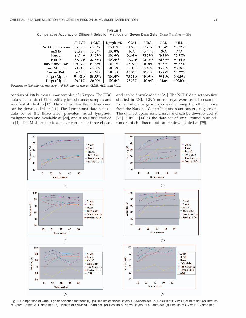
Fig. 1. Comparison of various gene selection methods (I). (a) Results of Naive Bayes: GCM data set. (b) Results of SVM: GCM data set. (c) Resultsof Naive Bayes: ALL data set. (d) Results of SVM: ALL data set. (e) Results of Naive Bayes: HBC data set. (f) Results of SVM: HBC data set.

6.2 Effectiveness of Gene Selection

Table 4 presents the accuracy values of applying SVM onthe top 30 genes selected by different methods and also onall the genes without selection. The accuracy values areobtained via 10-fold cross validation. The table shows thatgene selection improves classification performance; at leastthe accuracy of SVM on genes selected by both the D-optand A-opt methods outperform that without feature

selection. We will discuss the number of selected genes in

Section 6.4.

6.3 Performance of Different Gene SelectionMethods

In this section, we present a comparative study of various

gene selection methods using SVM and Naive Bayes

algorithms on the seven data sets. Both SVM and Naive


Fig. 2. Comparison of various gene selection methods (II). (a) Results of Naive Bayes: Lymphoma data set. (b) Results of SVM: Lymphoma data set.

(c) Results of Naive Bayes: MLL data set. (d) Results of SVM: MLL data set. (e) Results of Naive Bayes: NCI60 data set. (f) Results of SVM: NCI60

data set. (g) Results of Naive Bayes: SRBCT data set. (h) Results of SVM: SRBCT data set.

Bayes have been widely used in previous studies(e.g., [18]and [25]). Figs. 1 and 2 show the classification accuracyresults as a function of the number of selected genes on theseven data sets, respectively. From the comparative study,we observe the following:

. Gene selection by experimental design (D-opt andA-opt) outperforms other gene selection methodssuch as information gain, etc. It largely owes this tothe generality of the multivariate Gaussian genera-tive model. In addition, our methods estimate theinformation gain based on models, instead of on thedata itself. This overcomes the limitations of datasparseness and provides more robust and accurateestimations.

. The results of the A-opt method are similar to thoseof the D-opt method. Besides the simplicity of A-opt,the A-opt method outperforms the D-opt method inmost cases. There are some discussion of comparingA-optimality and D-optimality in the literatureexperimental designs [9].

. Gene selection by D-opt and A-opt implicitly selectsthe features with the minimum redundancy. Instep 6 of Algorithm 2 and step 5 of Algorithm 5,the covariance matrices are updated, which removesthe second-order redundancy. We can find similaractions in other algorithms as well.

6.4 Number of Selected Genes

From the above experiment, it can be observed that whenthe number of selected genes is greater than 30, the variationof the performance is small. In step 6 of Algorithm 4, weselect genes to reduce the generalized variance. In step 5 ofAlgorithm 7, we select genes to reduce the total variance.Figs. 3, 4, and 5 show the variance reduction as the functionof the number of genes on the seven data sets, respectively.The number of selected genes is varied from 1 to 50, and theresults show the change of classification accuracy.

The experiment results demonstrate that only a smallnumber of genes are needed for classification purposes. Inour experiments, we observe that when the number ofselected genes is greater than 30, the variation of theclassification performance is small. We find that thecumulative reduction in generalized variance or totalvariance converges after 30 steps.

6.5 Other Discussion

This set of experiments aims to study the choice of theregularization parameter � in our proposedA-opt andD-optmethods. We set the number of selected genes to be 30 andchange � from 0.1 to 0.9. Fig. 6 shows that the accuracy is notsensitive to the regularization parameter. Note that on theLYM and HBC data sets, the accuracies of both methods are100 percent under different regularization parameters. Inour experiments, we choose 0.5 as �.

7 DISCUSSIONS

Though we are studying the feature selection problem in thispaper, the idea largely owes to that of experimental designs.

In the statistics literature, the experimental designs can bebacktracked to the ideas presented in [15]. The goal ofexperimental designs is usually to extract the maximumamount of information from as few observations aspossible. For experimental designs, several criteria can be


Fig. 3. Variance reduction on data sets (I). (a) A-opt: GCM data set.

(b)D-opt: GCM data set. (c)A-opt: ALL data set. (d)D-opt: ALL data set.

Fig. 4. Variance reduction on data sets (II). (a) A-opt: HBC data set.(b) D-opt: HBC data set. (c) A-opt: Lymphoma data set. (d) D-opt:Lymphoma data set. (e) A-opt: MLL data set. (f) D-opt: MLL data set.

used, such as D-optimality and A-optimality [9]. They allconcern about reducing the uncertainties of estimatedparameters. The criterion of the D-optimality is minimizingthe generalized variance of the joint distribution ofparameters, i.e., the determinant of the multivariate variance,which gives its name. The criterion of the A-optimality isminimizing the average variance of all parameters.

As concentrating on the predictive variance of a targetset of data, Yu et al. [35] propose transductive experimentaldesigns for least squares linear (or kernel) regression. Theidea is to add samples to the training set in order toimprove the numerical stability of predictions on the targettest data, measured by the inversion of the Fisher informa-tion matrix. It has been shown that the predictive stabilityonly depends on the locations of the selected training data,while it does not depend on their label values, which leads toa very simple active learning approach [35].

Though there is a big difference between experimentaldesigns and feature selection at the first glance, we find aduality property between them.

Let us consider the problem of predicting target Y givena row of feature random vectors X. We assume that themodel is a linear model:

Y ¼ X>wþ �; ð21Þ

where w is the weight vector, and � is the error. The reasonfor using linear models is because linear models are simpleand scalable.

Given the training data y and X, where y is the columntarget vector and X is the feature matrix, each row of X is afeature vector. We can write (21) in matrix format as

y ¼ Xwþ ��;

where �� is the error vector.We further assume that the loss function is a square loss;

therefore, we want to minimize 12 ��>��. Meanwhile, we prefer

a robust estimation of w, i.e., a regularization term, �2 w>w.

Combining them, the estimation problem becomes

arg minw

1

2ðy�XwÞ>ðy�XwÞ þ �

2w>w: ð22Þ

Problem (22) can be explicitly solved as

bw ¼ ðX>Xþ �IÞ�1X>y: ð23Þ

This is also known as ridge regression.Given a feature vector x, the estimation of y is

by ¼ x>ðX>Xþ �IÞ�1X>y: ð24Þ

On the other hand, we can estimate y by the multivariate

Gaussian model. For simplicity, we assume that �� ¼ 0. By

(7), we know that

y ¼��T jF ¼ �TF ð�FF Þ�1x

¼y>XðX>Xþ �IÞ�1x;

which is equal to (24) as long as we have the same �.


Fig. 5. Variance reduction on data sets (III). (a) A-opt: NCI60 data set.

(b) D-opt: NCI60 data set. (c) A-opt: SRBCT data set. (d) D-opt: SRBCT

data set.

Fig. 6. Different regularization parameters on the seven data sets.(a) MLL data set. (b) NCI60 data set. (c) LYM data set. (d) GCM dataset. (e) HBC data set. (f) ALL data set. (g) SRBCT data set.

This shows the duality between the target label and thefeature. This property motivates us to treat the featureselection as a dual problem of selecting data samples tolabel in active learning or experimental designs. Then, wecan apply experimental design approaches, more preciselytransductive experimental design [35], onto the feature selec-tion problem.

8 CONCLUSIONS

In this paper, we suggest multivariate Gaussian generativemodels for feature (gene) selection because multivariatenormal (Gaussian) distributions are a maximum-entropyprobability distribution. Using the model-based entropyestimation, we avoid the data sparseness problem thatcommonly happens in the empirical information gainapproach.

Using the properties of multivariate normal distribu-tions, we derive the feature selection methods based onthe D-optimality criterion and its approximation, theA-optimality criterion.

To efficiently select genes from gene expression data,where the numbers of features are large and the numbers ofsamples are relatively small, we propose several simplealgorithms (a few lines of code). Among them, Algorithm 4and Algorithm 7 are most suitable for gene expression data.The time complexity of the proposed algorithms is linear tothe product of the number of genes and the number ofsamples for each iteration of selection.

The experiments on seven gene data sets and thecomparison with other five approaches show the accuracyand efficiency of our approach.

ACKNOWLEDGMENTS

The authors would like to thank NIH/NIGMS S06GM008205, US NSF IIS-0546280, and DBI-0850203 forpartially supporting this work.

REFERENCES

[1] A.A. Alizadeh, M.B. Eisen, R.E. David, C. Ma, I.S. Lossos,A.R. osenwald, H.C. Boldrick, H. Sabet, T. Tran, X. Yu, J.I. Powell,L. Yang, G.E. Martu, T. Moore, J. Hudson, L. Lu, D.B. Lewis,R. Tibshirani, G. Sherlock, W.C. Chan, T.C. Greiner,D.D. Weisenburger, G.P. Armitage, R. Warnke, R. Levy,W. Wilson, M.R. Grever, J.C. Byrd, D. Botsten, P.O. Brown, andL.M. Staudt, “Distinct Types of Diffuse Large B-Cell LymphomaIdentified by Gene Expression Profiling,” Nature, vol. 403, pp. 503-511, 2000.

[2] ALL, http://www.stjuderesearch.org/data/ALL1/, 2008.[3] C. Bishop, Pattern Recognition and Machine Learning. Springer,

2006.[4] C.-C. Chang and C.-J. Lin, “LIBSVM: A Library for Support Vector

Machines,” http://www.csie.ntu.edu.tw/~cjlin/libsvm, 2001.[5] M. Chee, R. Yang, E. Hubbell, A. Berno, X. Huang, D. Stern,

J. Winkler, D. Lockhart, M. Morris, and S. Fodor, “AccessingGenetic Information with High Density DNA Arrays,” Science,vol. 274, pp. 610-614, 1996.

[6] T. Cover and J. Thomas, Elements of Information Theory. John Wiley& Sons, 1991.

[7] T. Cover, “The Best Two Independent Measurements Are Not theTwo Best,” IEEE Trans. Systems, Man, and Cybernetics, vol. 4,pp. 116-117, 1974.

[8] S. Dudoit, J. Fridlyand, and T.P. Speed, “Comparison ofDiscrimination Methods for the Classification of Tumors UsingGene Expression Data,” J. Am. Statistical Assoc., vol. 97, no. 457,pp. 77-87, 2002.

[9] V.V. Fedorov, Theory of Optimal Experiments. Academic Press,1972.

[10] S. Fodor, J. Read, M. Pirrung, L. Stryer, A. Lu, and D. Solas,“Light-Directed, Spatially Addressable Parallel ChemicalSynthesis,” Science, vol. 251, pp. 767-783, 1991.

[11] HBC, http://www.columbia.edu/~xy56/project.htm, 2007.[12] I. Hedenfalk, D. Duggan, Y.C. Radmacher, M. Bittner, M. Simon,

R. Meltzer, P. Gusterson, B. Esteller, M. Kallioniemi, B.W. Borg,and A. Trent, “Gene-Expression Profiles in Hereditary BreastCancer,” New England J. Medicine, vol. 344, no. 8, pp. 539-548,2001.

[13] E.T. Jaynes, “Information Theory and Statistical Mechanics,”Physical Rev., vol. 106, no. 4, pp. 620-630, May 1957.

[14] J. Khan, J. Wei, M. Ringner, L. Saal, M. Ladanyi, F. Westermann,F. Berthold, M. Schwab, C.R. Antonescu, C. Peterson, andP. Meltzer, “Classification and Diagnostic Prediction of CancersUsing Expression Profiling and Artificial Neural Networks,”Nature Medicine, vol. 7, no. 6, pp. 673-679, 2001.

[15] J. Kiefer, “Optimum Experimental Designs,” J. Royal StatisticalSoc. B, vol. 21, pp. 272-319, 1959.

[16] R. Kohavi and G.H. John, “Wrappers for Feature SubsetSelection,” Artificial Intelligence, vol. 97, no. 1-2, pp. 273-324,1997.

[17] P. Langley, “Selection of Relevant Features in Machine Learning,”Proc. AAAI Fall Symp. Relevance, pp. 140-144, 1994.

[18] T. Li, C. Zhang, and M. Ogihara, “A Comparative Study of FeatureSelection and Multiclass Classification Methods for TissueClassification Based on Gene Expression,” Bioinformatics, vol. 20,no. 15, pp. 2429-2437, 2004.

[19] Y. Li, C. Campbell, and M. Tipping, “Bayesian AutomaticRelevance Determination Algorithms for Classifying Gene Ex-pression Data,” Bioinformatics, vol. 18, pp. 1332-1339, 2004.

[20] LYM, http://genome-www.stanford.edu/lymphoma, 2008.[21] MLL, http://research.dfci.harvard.edu/korsmeyer/MLL.htm,

2008.[22] R. Marko and K. Igor, “Theoretical and Empirical Analysis of

ReliefF and RReliefF,” Machine Learning J., pp. 23-69, 2003.[23] NCI60, http://genome-www.stanford.edu/nci60/, 2008.[24] C. Ooi and P. Tan, “Genetic Algorithms Applied to Multi-Class

Prediction for the Analysis of Gene Expression Data,” Bioinfor-matics, vol. 19, pp. 37-44, 2003.

[25] H. Peng, F. Long, and C. Ding, “Feature Selection Based on MutualInformation: Criteria of Max-Dependency, Max-Relevance, andMin-Redundancy,” IEEE Trans. Pattern Analysis and MachineIntelligence, vol. 27, no. 8, pp. 1226-1238, Aug. 2005.

[26] K.B. Petersen and M.S. Pedersen, The Matrix Cookbook,Version 20051003, 2006.

[27] S. Ramaswamy, P. Tamayo, R. Rifkin, S. Mukherjee, C.-H. Yeang,M. Angelo, C. Ladd, M. Reich, E. Latulippe, J.P. Mesirov,T. Poggio, W. Gerald, M. Loda, E.S. Lander, and T. R.Golub,“Multiclass Cancer Diagnosis Using Tumor Gene ExpressionSignatures,” vol. 98, no. 26, pp. 15149-15154, 2001.

[28] D.T. Ross, U. Scherf, M.B. Eisen, C.M. Perou, C. Rees,P. Spellmand, V. Iyer, S.S. Jeffrey, M. Van de Rijn, M. Waltham,A. Pergamenschikov, J.C.F. Lee, D. Lashkari, D. Shalon,T.G. Myers, J.N. Weinstein, D. Botstein, and M.P.O. Brown,“Systematic Variation in Gene Expression Patterns in HumanCancer Cell Lines,” Nature Genetics, vol. 24, pp. 227-235, 2000.

[29] SRBCT, http://research.nhgri.nih.gov/microarray/Supplement/,2008.

[30] C. Stein, “Estimation of a Covariance Matrix,” Rietz Lecture, 39thIMS Ann. Meeting, 1975.

[31] Y. Su, T.M. Murali, V. Pavlovic, and S. Kasif, “Rankgene:Identification of Diagnostic Genes Based on Expression Data,”Bioinformatics, http://genomics10.bu.edu/yangsu/rankgene/,2003.

[32] E.P. Xing, M.I. Jordan, and R.M. Karp, “Feature Selection forHigh-Dimensional Genomic Microarray Data,” Proc. 18th Int’lConf. Machine Learning (ICML ’01), pp. 601-608, 2001.

[33] E.-J. Yeoh, M.E. Ross, S.A. Shurtleff, W.K. williams, D. Patel,R. Mahrouz, F.G. Behm, S.C. Raimondi, M.V. Relling, A. Patel,C. Cheng, D. Campana, D. Wilkins, X. Zhou, J. Li, H. Liu,C.-H. Pui, W.E. Evans, C. Naeve, L. Wong, and J.R. Downing,“Classification, Subtype Discovery, and Prediction of Outcome inPediatric Lymphoblastic Leukemia by Gene Expression Profiling,”Cancer Cell, vol. 1, no. 2, pp. 133-143, 2002.

[34] K.Y. Yeung, C. Fraley, A. Murua, A.E. Raftery, and W.L. Ruzzo,“Model-Based Clustering and Data Transformations for GeneExpression Data,” Bioinformatics, vol. 17, no. 10, pp. 977-987, 2001.


[35] K. Yu, J. Bi, and V. Tresp, “Active Learning via TransductiveExperimental Design,” Proc. 23rd Int’l Conf. Machine Learning(ICML ’06), pp. 1081-1088, 2006.

[36] L. Yu, H. Liu, and V. Tresp, “Redundancy Based Feature Selectionfor Microarray Data,” Proc. 10th Int’l Conf. Knowledge Discovery andData Mining (KDD), 2004.

Shenghuo Zhu received the BE degree fromZhejiang University in 1994, the BE degreefrom Tsinghua University in 1997, and thePhD degree in computer science from theUniversity of Rochester in 2003. He is aresearch staff member at NEC LaboratoriesAmerica, Cupertino, California. His primaryresearch interests include information retrieval,probabilistic modeling, machine learning, anddata mining.

Dingding Wang received the bachelor’s degreefrom the Department of Computer Science,University of Science and Technology of China,in 2003. She is currently a PhD student in theSchool of Computer Science, Florida Interna-tional University, Miami. Her research interestsare data mining, information retrieval, andmachine learning.

Kai Yu received the PhD degree in computerscience from the University of Munich, Germany,in 2004. He worked at Siemens as a seniorresearch scientist during 2004-2006. He iscurrently a research staff member at NECLaboratories America, Cupertino, California. Hisresearch has been focused on probabilisticmodeling, Bayesian inference, Gaussian pro-cesses, general machine learning algorithms,and their applications to information retrieval, text

mining, recommender systems, clinical data analysis, intrusion detection,and visual recognition. He is the author of more than 40 research papersin international conferences and journals and has served as a programcommittee member or reviewer for conferences like ICML, NIPS, SIGIR,and ECML.

Tao Li received the PhD degree in computerscience from the Department of ComputerScience, University of Rochester, in 2004. Heis currently an associate professor in the Schoolof Computer Science, Florida International Uni-versity, Miami. His research interests are datamining, machine learning, information retrieval,and bioinformatics.

Yihong Gong received the BS, MS, and PhDdegrees in electronic engineering from theUniversity of Tokyo in 1987, 1989, and 1992,respectively. He then joined the NanyangTechnological University of Singapore, wherehe worked as an assistant professor in theSchool of Electrical and Electronic Engineeringfor four years. From 1996 to 1998, he worked atthe Robotics Institute, Carnegie Mellon Univer-sity, as a project scientist. He was a principal

investigator for both the Informedia Digital Video Library Project and theExperience-on-Demand Project funded in multimillion dollars by USNSF, DARPA, NASA, and other government agencies. In 1999, hejoined NEC Laboratories America and has been leading the MultimediaProcessing Group since then. In 2006, he became the site manager tolead the Cupertino branch of the laboratories. His research interestsinclude multimedia content analysis and machine learning applications.The major research achievements from his group include news videosummarization, sports highlight detection, data clustering, and Smart-Catch video surveillance that led to a successful spin-off.

. For more information on this or any other computing topic,please visit our Digital Library at www.computer.org/publications/dlib.


IEEE/ACM TRANSACTIONS ON COMPUTATIONAL …users.cis.fiu.edu/~taoli/pub/feature-tcbb.pdf ·...

Documents

Transcript of IEEE/ACM TRANSACTIONS ON COMPUTATIONAL …users.cis.fiu.edu/~taoli/pub/feature-tcbb.pdf ·...