IEEE TRANSACTIONS ON SIGNAL PROCESSING, …jchoi/files/papers/JXCJW_TSP2013.pdfimation techniques...

IEEE TRANSACTIONS ON SIGNAL PROCESSING, VOL. 61, NO. 2, JANUARY 15, 2013 223

Gaussian Process Regression for Sensor NetworksUnder Localization Uncertainty

Mahdi Jadaliha, Yunfei Xu, Jongeun Choi, Nicholas S. Johnson, and Weiming Li

Abstract—In this paper, we formulate Gaussian process regres-sion with observations under the localization uncertainty due to theresource-constrained sensor networks. In our formulation, effectsof observations, measurement noise, localization uncertainty, andprior distributions are all correctly incorporated in the posteriorpredictive statistics. The analytically intractable posterior predic-tive statistics are proposed to be approximated by two techniques,viz., Monte Carlo sampling and Laplace’s method. Such approx-imation techniques have been carefully tailored to our problemsand their approximation error and complexity are analyzed. Sim-ulation study demonstrates that the proposed approaches performmuch better than approaches without considering the localizationuncertainty properly. Finally, we have applied the proposed ap-proaches on the experimentally collected real data from a dye con-centration field over a section of a river and a temperature field ofan outdoor swimming pool to provide proof of concept tests andevaluate the proposed schemes in real situations. In both simula-tion and experimental results, the proposed methods outperformthe quick-and-dirty solutions often used in practice.

Index Terms— Gaussian processes, Monte Carlo methods, re-gression analysis, sensor networks, Laplace’s methods.

I. INTRODUCTION

R ECENTLY, there has been a growing interest in wirelesssensor networks due to advanced embedded network

technology. Their applications include, but are not limitedto, environment monitoring, building comfort control, trafficcontrol, manufacturing and plant automation, and surveillance

Manuscript received April 20, 2012; accepted September 28, 2012. Date ofpublication October 09, 2012; date of current version December 20, 2012. Theassociate editor coordinating the review of this manuscript and approving it forpublication was Dr. Z. Jane Wang. This work has been supported, in part, by theNational Science Foundation through CAREER Award CMMI-0846547. Thisarticle is Contribution 1713 of the U.S. Geological Survey Great Lakes ScienceCenter. In-stream field experiments were supported by the Great Lakes FisheryCommission. The work of W. Li was supported in part by the National ScienceFoundations Awards IOB0517491 and IOB0450916. This support is gratefullyacknowledged. Use of trademark names does not represent endorsement by theU.S. Government.M. Jadaliha and Y. Xu are with the Department of Mechanical Engineering,

Michigan State University, MI 48824 USA (e-mail: [email protected];[email protected]).J. Choi is with the Departments of Mechanical Engineering and Electrical

and Computer Engineering, Michigan State University, MI 48824 USA (e-mail:[email protected]).N. S. Johnson is with United States Geological Survey, Great Lakes Science

Center, Hammond Bay Biological Station, Millersburg, MI 49759 USA (e-mail:[email protected]).W. Li is with the Department of Fisheries and Wildlife, Michigan State Uni-

versity, East Lansing, MI 48824 USA (e-mail: [email protected]).Color versions of one or more of the figures in this paper are available online

at http://ieeexplore.ieee.org.Digital Object Identifier 10.1109/TSP.2012.2223695

systems [1], [2]. Mobility in a sensor network can increase itssensing coverage both in space and time, and robustness againstuncertainties in environments. Exploitation of mobile sensornetworks has been increased in collecting spatio-temporal datafrom the environment [3]–[5].Gaussian process regression (or Kriging in geostatistics)

has been widely used to draw statistical inference from geo-statistical and environmental data [6], [7]. Gaussian processmodeling enables us to predict physical values, such as temper-ature or harmful algae bloom biomass, at any point and timewith a predicted uncertainty level. For example, near-optimalstatic sensor placements with a mutual information criterionin Gaussian processes were proposed in [8], [9]. A distributedKriged Kalman filter for spatial estimation based on mobilesensor networks was developed in [5]. Centralized and dis-tributed navigation strategies for mobile sensor networks tomove in order to reduce prediction error variances at points ofinterest were developed in [10].Localization in sensor networks is a fundamental problem in

various applications to correctly fuse the spatially collected dataand estimate the process of interest. However, obtaining pre-cise localization of robotic networks under limited resources isvery challenging [11], [12]. Among the localization schemes,the range-based approach [13], [14] provides higher precisionas compared to the range-free approach that could be cost-ef-fective. The global positioning system (GPS) becomes one ofthe major absolute positioning systems in robotics and mobilesensor networks. Most of affordable GPSs slowly update theirmeasurements and have resolution worse than onemeter. AGPSis often augmented by the inertial navigation system (INS) forbetter resolution [15]. In practice, resource-constrained sensornetwork systems are prone to large uncertainty in localization.Most previous works on Gaussian process regression for mobilesensor networks [6], [9], [10], [16] have assumed that the exactsampling positions are available, which is not practical in realsituations.Therefore, motivated by the aforementioned issues, we con-

sider correct (Bayesian) integration of uncertainties in samplingpositions, and measurements noise for Gaussian process regres-sion and its computation error and complexity analysis for thesensor network applications. The overall picture of our work issimilar to the one in [17] in which an extended Kalman filter(EKF) was used to incorporate robot localization uncertaintyand field parameter uncertainty. However, [17] relies on a para-metric model, which is a radial basis function network modeland EKF, while our motivation is to use more flexible non-para-metric approach, viz., Gaussian process regression taking intoaccount localization uncertainty in a Bayesian framework.

1053-587X/$31.00 © 2012 IEEE

224 IEEE TRANSACTIONS ON SIGNAL PROCESSING, VOL. 61, NO. 2, JANUARY 15, 2013

Fig. 1. The prediction results of applying Gaussian process regression on the true and noisy sampling position are shown. The first, second, and third rowscorrespond to the prediction, prediction error variance, and squared empirical error (between predicted and true fields) fields. The first column shows the result ofapplying Gaussian process regression on the true sampling positions. Second and third columns show the results of applying Gaussian process regression on thenoisy sampling positions with and noise covariance matrices, respectively. True and noisy sampling positions are shown in circles withagent indices in the second row.

Gaussian process regression in [18] integrate uncertainty inthe test input position for multiple-step ahead time series fore-casting. In [18], uncertainty was not considered in the samplingpositions of the training data (or observations).However, localization uncertainty effect is potentially signifi-

cant. For example, Fig. 1 shows the effect of noisy sampling po-sitions on the results of Gaussian process regression. Note thatadding noise to the sampling positions considerably increase theempirical RMS error, shown in the third row of Fig. 1.A Gaussian approximation to the intractable posterior pre-

dictive statistics obtained in [18] has been utilized for the pre-dictive control with Gaussian models [19], [20] and Gaussianprocess dynamic programming [21]. In general, the length ofthe training data is much longer than that of the test point forsensor network applications, therefore, our problem possibly in-volves a high dimensional uncertainty vector for the samplingpositions.Gaussian process prediction with localization uncertainty can

be obtained as a posterior predictive distribution using Bayes’rule. The main difficulty to this is that it has no analytic closed-form solution and has to be approximated either through MonteCarlo sampling [22] or other approximation techniques suchas variational inference [23]. As an important analytical ap-proximation technique, Laplace’s method has been known tobe useful in many such situations [24], [25]. Different Laplaceapproximation techniques have been analyzed in terms of ap-proximation error and computation complexity [24]–[27].The contribution of this paper is as follows. First, we for-

mulate Gaussian process regression with observations underthe localization uncertainty due to the resource-constrained

(possibly mobile) sensor networks. Next, approximations havebeen obtained for analytically intractable predictive mean, andpredictive variance by using the Monte Carlo sampling andLaplace’s method. Such approximation methods have beencarefully tailored to our problems. In particular, a modified ver-sion of the moment generating function (MGF) approximation[25] has been developed as a part of Laplace’s method to reducethe computational complexity. In addition, we have analyzedand compared the approximation error and the complexityso that one can choose a tradeoff between the performancerequirements and constrained resources for a particular sensornetwork application. Another important contribution has beento provide proof of concept tests and evaluate the proposedschemes in real situations. We have applied the proposed ap-proaches on the experimentally collected real data from a dyeconcentration field over a section of a river and a temperaturefield of an outdoor swimming pool.The preliminary work of this paper containing only the

Laplace methods along with simulation results was reported in[28].The remainder of this paper is organized as follows. In

Section II, we review Gaussian process regression, MonteCarlo sampling and Laplace’s method briefly. In Section III,Gaussian process prediction in the presence of the localizationuncertainty has been formulated for a proposed samplingscheme as a Bayesian inference problem. We first presentthe Monte Carlo estimators for the posterior predictive meanand variance in Section IV. In Section V, using Laplace’smethod, we provide approximations for the posterior predictivestatistics. Section VI compares the computational cost and

JADALIHA et al.: GAUSSIAN PROCESS REGRESSION FOR SENSOR NETWORKS UNDER LOCALIZATION UNCERTAINTY 225

approximation accuracy over the proposed estimators basedon the Mont Carlo sampling and the Laplace’s method. Fi-nally the simulation and experimental results are provided inSections VII and VIII, respectively.Standard notation will be used throughout the paper. Let ,, , , , denote, respectively, the sets of real,

non-negative real, positive real, integer, non-negative integer,and positive integer numbers. denotes the identity matrixof size ( for an appropriate dimension.) For column vec-tors , , and ,

stacks all vectors to create one columnvector, and denotes the Euclidean norm (or the vector2-norm) of . denotes the determinant of a matrix

, and denotes trace of a square matrix . Letand denote, respectively, the expectation and the vari-ance of a random vector . A random vector , whichis distributed by a multivariate Gaussian distribution of a mean

and a variance , is denoted by .We define the first and the second derivative operators on

with respect to a vector as follow.

.... . .

...

If there exists and , such that the approximation errorsatisfies , we say that the error betweenand is of order and also write . Other

notation will be explained in due course.

II. PRELIMINARIES

In this section, we review the spatio-temporal Gaussianprocess, Monte Carlo sampling and Laplace’s method, whichwill be used throughout the paper.

A. Gaussian Process Regression

A Gaussian process defines a distribution over a space offunctions and it is completely specified by its mean functionand covariance function. Let denotethe index vector, where contains the sampling lo-cation and the sampling time . AGaussian process, , is formally defined as below.Definition 1: AGaussian process [7] is a collection of random

variables, any finite number of which have a joint Gaussian dis-tribution.For notational simplicity, we consider a zero-mean Gaussian

process1 . For example, one mayconsider a covariance function defined as

(1)

1A Gaussian process with a nonzero-mean can be treated by a change of vari-ables. Even without a change of variables, this is not a drastic limitation, sincethe mean of the posterior process is not confined to zero [7].

where . In general, the mean and the covariance func-tions of a Gaussian process can be estimated a priori by maxi-mizing the likelihood function [16].Suppose, we have noise corrupted observations without lo-

calization error, and . Assumethat , where is an independent andidentically distributed (i.i.d.) white Gaussian noise with vari-ance . is defined by . The col-lections of the realizations and the

observations have the Gaussian dis-tributions

where is the covariance matrix of obtained by, and is the identity matrix with an

appropriate size. We can predict the value of the Gaussianprocess at a point as [7]

(2)

In (2), the predictive mean is

(3)

and the predictive variance is given by

(4)where is the covariance matrix between andobtained by , and isthe variance at . (3) and (4) can be obtained from the fact that

(5)

Note that the predictive mean in (3) and its prediction errorvariance in (4) require the inversion of the covariance matrixwhose size depends on the number of observations . Hencea drawback of Gaussian process regression is that its computa-tional complexity and memory space increase as more measure-ments are collected, making the method prohibitive for agentswith limited memory and computing power. To overcome thisincrease in complexity, a number of approximation methodsfor Gaussian process regression have been proposed. In partic-ular, the sparse greedy approximation method [29], the Nystrommethod [30], the informative vector machine [31], the likeli-hood approximation [32], and the Bayesian committee machine[33] have been shown to be effective for many problems.In particular, it has been proposed that spatio-temporal

Gaussian process regression can be applied to truncated obser-vations including only measurements near the target positionand time of interest for agents with limited resources [10]. Tojustify prediction based on only the most recent observations, asimilar argument has been made in [34] in the sense that the datafrom the remote past do not change the predictors significantlyunder the exponentially decaying correlation functions.In this paper, we also assume that at each iteration the mobile

sensor networks only needs to fuse a fixed number of truncated


observations, which are near the target points of interest, to limitthe computational resources.

B. Monte Carlo and Importance Sampling

In what follows, we briefly review Monte Carlo and Impor-tance sampling based on [35]. The idea of Monte Carlo sim-ulation is to draw an i.i.d. set of random samplesfrom a target density , where . Theserandom samples will be used to approximate by an empir-ical point-mass function , where

denotes the Dirac delta. Consequently, the integralscan be approximated with tractable sums that convergeas follows.

is an unbiased estimator. In addition, it will almost surelyasymptotically converge to , which can be proved by thestrong law of large numbers. Considering forsimplicity, if satisfies ,

then the variance of the estimator converges to asincreases. In particular, the central limit theorem provides

us with convergence in distribution as follows., where denotes convergence in distri-

bution.Importance sampling is a special case of Monte Carlo

implementation, having random samples generated from anavailable distribution rather than the distribution of interest.Let us introduce an arbitrary importance proposal distribution

whose support includes the support of . We canthen rewrite as , where

is known as the importance weight. Simulating

i.i.d. samples according to and evaluating, a possible unbiased Monte Carlo estimate of is

given by .

Under weak assumptions, the strong law of large num-bers applies, yielding . This integration

method can also be interpreted as a sampling methodwhere the posterior density is approximated by

, and is the integra-

tion of with respect to the empirical measure .In this paper, we shall compute the ratio of two integrals in

the form of

(6)

where , and are defined on a space . To com-pute in (6), we use the following approximation as pro-posed in [36].

(7)

where is a sequence of i.i.d. random vectors,which is drawn from distribution.In the following theorem, which can be shown to be a special

case of the results from [36], we show the convergence proper-ties of the approximation in (7) as functions of , the number ofrandom samples [36].Theorem 2: (Theorems 1 and 2 from [36]) Consider the

approximation given in (7) to the ratio givenin (6). If is proportional to a proper probabilitydensity function defined on , and , and

are finite, we have

where

Proof: It is a straightforward application of the results fromTheorems 1 and 2 in [36] to (6) and (7).

C. Laplace Approximations

The Laplace method is a family of asymptotic approxima-tions that approximate an integral of a function, i.e., ,where , and . Let the function be ina form , where , andis a two times continuously differentiable real function on .Let denote the exact mode of , i.e.,

Then Laplace’s method produces the approximation [24]:

(8)

where . The Laplace approximation in (8)will produce reasonable results as long as the is unimodalor at least dominated by a single mode.In practice it might be difficult to find the exact mode of .

A concept of an asymptotic mode is introduced to gauge theapproximation error when the exact mode is not used [26].Definition 3: is called an asymptotic mode of order

for if as , and.

Suppose that is an asymptotic mode of orderfor and satisfies the regularity conditions given inAppendix A. Then it follows that we have

(9)where is given by


More precise form with the asymptotic mode of orderis computed for an approximation of order in

[27].In many Bayesian inference applications and as in our

problem, we need to compute the ratio of two integrals. Tothis end, fully exponential Laplace approximations has beendeveloped by [24] to compute Laplace approximations of theratio of two integrals, i.e.,

(10)

If each of and has a dominant peak at its maximum, thenLaplace’s method may be directly applied to both the numeratorand denominator of (10) separately. If the regularity conditionsare satisfied, using (8) for the denominator approximation and(9) for the numerator approximation, Miyata [26] obtained thefollowing approximation and its error order,

(11)

where is the exact mode of , and is the asymptotic modeof , and

(12)

Laplace approximations typically has an error of orderas shown in (8) and (9). On the other hand, fully exponentialLaplace approximations for the ratio form yield an error of order

as shown in (11) since the error terms of orderin the numerator and denominator cancel each other [24].Fully exponential Laplace approximations which are pre-

sented in (11) is limited for positive functions. Then, Tierneyet al. [25] proposed a second-order approximation to the ex-pectation of a general function (not necessarily positive)by applying the fully exponential method to approximate

and then differentiating the approxi-mated . Consider is defined as follow

where , and is positive, whilecould be positive or negative. In particular, eval-

uated at yields a second-order approximation toand its order of the error as follow.

(13)

This method, which is called moment generating function(MGF) Laplace approximation, gives a standard-form approxi-mation using the exact mode of [25].Miyata [26], [27] extended the MGF method for one without

computing the exact mode of . Let be an asymptoticmode of order for . Suppose that satisfiesthe regularity conditions for the asymptotic-mode Laplace

method. By using Theorem 5 in [26], the approximation ofand its error order are given as

(14)

where is the -th row, -th column element of the matrix. Furthermore, if is the exact mode of , then the

approximation has a simpler form because the terms that includevanish

(15)

III. THE PROBLEM STATEMENT

In practice, (data with perfect localization) is not avail-able due to localization uncertainty, and instead its exact sam-pling points will be replaced with noise corrupted samplingpoints. To average out measurement and localization noises,in this paper, we propose to use a sampling scheme in whichmultiple measurements are taken repeatedly at a set of sam-pling points of a sensor network. For robotic sensors or mo-bile sensor networks, this sampling strategy could be efficientand inexpensive since the large energy consumption is usuallydue to the mobility of the sensor network. Let sensing agentsbe indexed by . From the proposed samplingscheme, we assume that each agent takes multiple data pairs

, which are indexed by ata set of sampling points by the sensor network .We then define the map that takes the index ofthe data pair in as the input and returns the index of the sensorthat produced the data pair as the output. Consider the followingrealizations using the sampling scheme and the notation just in-troduced.

where is an i.i.d. white Gaussian noise with a zero meanand a variance of , i.e., and is a lo-calization error which has a multivariate normal distributionwith a zero mean and a covariance matrix , i.e.,

. For instance, the distribution of the localiza-tion error may be a result of the fusion of GPS and INSmeasure-ments [15], or landmark observations and robot’s kinematics[37].To simplify the notation, is introduced to denote the data

with the measurement noise and localization error as follows.

(16)


We also define the collective sampling point vectors with andwithout localization uncertainty, and the cumulative localizationnoise vector, respectively by

(17)

From the proposed sampling scheme, to average out the mea-surement and localization uncertainties, the number of measure-ments can be increased without increasing the number of sen-sors , and consequently without increasing the dimension of

. Hence, this approach may be efficient for the re-source-constrained (mobile) sensor network at the cost of takingmore measurements. Using collective sampling point vectors in(17), we have the following relationship.

(18)

where , and if, otherwise .

The conditional probabilities and can be ex-pressed as

where . From a Bayesian perspective,we can treat as a random vector to incorporate a prior distri-bution on . For example, if we assign a prior distribution onsuch that then we have

(19)

where and .Evaluating posterior predictive statistics such as the density,

the mean, and the variance are of critical importance for thesensor network applications.Therefore, given the data in (16), our goal is to compute

the posterior predictive statistics. In particular we focused onthe following two quantities given in detail.• The predictive mean estimator (PME) is given by

.

(20)

where is given by (3).• The predictive variance estimator (PVE) is obtained simi-larly. From the following equation,

where , we obtaingiven as the following formula.

(21)

where is given by (4).The main challenge to our problems is the fact that there are

no closed-form formulas for the posterior predictive statisticslisted in (20), and (21). Therefore, in this paper, approximationtechniques will be carefully applied to obtain approximate solu-tions. In addition, the tradeoffs between the computational com-plexity and the precision will be investigated for the sensor net-works with limited resources.From (19), one might be tempted to use the best estimate of, e.g., the conditional expectation of for given measured lo-cations , i.e., for Gaussian process regression. Com-parison between these type of quick-and-dirty solutions and theproposed Bayesian approaches will be evaluated and discussedwith simulated and experimental data presented in Sections VIIand VIII, respectively.

IV. THE MONTE CARLO METHOD

In this section, we propose importance sampling to computethe posterior predictive statistics. We also summarize the con-vergence results of the MC estimators based on Theorem 2.

A. Predictive Mean

The predictive mean estimator is given by (20). Using im-portance sampling to approximate (20) leads to the followingequation,

(22)

Theorem 2 and (22) lead to

where ,is calculated from (3), and has been sampled fromgiven by (19).

B. Predictive Variance

For the prediction error variance given by (21), we have

Thus, we propose the following estimator.

(23)


where ,are obtained from the formulas similar to (4) and (3), and

is given by (22).Applying Theorem 2 for

, , and , we obtain thefollowing results.

where ,, and

Remark 4: Since is not available in (23),is used instead. Subsequently, the convergence results for

are given with respect to which con-verges to as by the definition.

V. FULLY EXPONENTIAL LAPLACE APPROXIMATIONS

In this section, we propose fully exponential Laplace approx-imations to compute the posterior predictive statistics. In theprocess of applying Laplace approximations, we also obtain theestimation of the sampling points given as a by-product. Fromthe observations given by (16), we can update the estimatesof the sampling points . To this end, we use the maximum aposteriori probability (MAP) estimate of given by

(24)

A. Perdictive Mean

The predictive mean estimator, given by (20), can be ap-proximated using MGF method (14). To compute , let

. Using

(25)

the predictive mean estimation using MGF method (MGF-PME), and its error order are given as

(26)

where is given in (14) or (15). However, theMGF-PMEgiven by (26) needs the computation of the third derivative of, which increases the complexity of the algorithm.In this paper, another MGF method has been developed in

order not to use the third derivative of . To approximate thederivative of at a point in (13), we utilize a three-pointestimation, which is the slope of a nearby secant line through thepoints and . Approximatingthe derivative in (13) with the three-point estimation, we canavoid the third derivative in (14) or (15). We summarize ourresults in the following theorem.

Theorem 5: Let be the exact mode of . The three-point predictive mean estimator (TP-PME) and its order of theerror are given by

(27)

where is given by (25), and we have used the followingdefinitions

Proof: First we use the three-point method to approximatederivative such that

Plugging into the above equationand using (13), we obtain

(28)By selecting , we recover the order of the error

. By computing the esti-

mates and in (28) using (11), (27) is obtained.Remark 6: The complexity of either (14) or (15) is

while the complexity of (27) is . In return, the error of (15)

is of order and the error of (27) is of order .

B. Predictive Variance

We now apply Laplace’s method to approximate the predic-tion error variance in a similar way. The prediction error vari-ance is given by (21). In this case, is given by (25) and

. Ap-plying (11) to this case, the approximate of and itsorder of the error are given by

(29)

where is the exact mode of , and is the asymptotic modeof . and are given by (12) and is givenby (27).


C. Simple Laplace Approximations

To minimize the computational complexity, one may prefer asimpler approximation. In this paper, we propose such a simpleapproximation at the cost of precision, which is summarized inthe following theorem.Theorem 7: Let be an asymptotic mode of order

for given by (25). Assume that satisfies the regularityconditions. Consider the following approximations forand

(30)

(31)

where and are covariance matrices as in (3) but ob-tained with .We have then the following order of errors.

Proof: The approximation for given by (30) is thefirst term of (14) neglecting high order terms. The second andthird terms in (14) have inside. is an asymptotic modeof order for . By Definition 3, the last term of (14)that contains is . Hence, without these high orderterms, we obtain a simpler approximation of order .The approximation for given by (31) can be

obtained by approximating (21) with the first term of the MGFapproximation. Let , then

. Using the first term of MGF,

and using , we obtain. The procedure of showing the

order of the approximation error is the same as what was shownfor the approximation in (30).Remark 8: Note that the simple Laplace predictive mean and

variance estimators in (30) and (31) take the same forms of theoriginal predictive mean and variance without the localizationerror, respectively given in (3) and (4), evaluated at theMAP es-timator of . As we previously mentioned, is the mode ofgiven by (25) and is the MAP estimator of , i.e., asdefined in (24). Therefore, the difference in the simple Laplaceapproximations with respect to a quick-and-dirty solution inwhich the measured location vector is used is that the simpleLaplace approximations use instead of .In applying Laplace’s method, using the one step Newton gra-

dient method to compute asymptotic modes, e.g., required in(29) or and required in (27) may not satisfy the regularityconditions. In this case, one needs to continue the Newton gra-dient optimization until the regularity conditions are satisfied.

VI. ERROR AND COMPLEXITY ANALYSIS

In this section, we analyze the order of the error and the com-putational complexity for the proposed approximation methods,which are summarized in Table I. A tradeoff between the ap-proximation error and complexity can be chosen taking into ac-count the performance requirements and constrained resourcesfor a specific sensor network application.

TABLE IERROR AND COMPLEXITY ANALYSIS

Fig. 2. A realization of the Gaussian process-ground truth.

For Laplace’s method, the order of the error ranges fromto at the cost of complexity from toas shown in Table I.

For the Monte Carlo estimators, we introduce , whichis the probabilistic error order and it implies that the estimationerror converges to in distribution as the number ofrandom samples increases. Therefore it is not appropriate tocompare the error bound between Monte Carlo and Laplace’smethod exactly. Monte Carlo algorithms are used for multi-variate integration of dimension . The probabilistic errororder of Monte Carlo algorithms that use sample evaluationsis of order for a given . We may assume that the order ofthe error for Monte Carlo methods do not depend on the numberof measurements for a large [36]. With this assumption, thenumber of samples needed forMonte Carlo algorithms to reducethe initial probabilistic error by is of order . Thecomplexity of the Monte Carlo methods, for the investigatedproblems in this paper, is . To achieve the probabilisticerror order , the complexity of Monte Carlo methodshas to be . If we want to keep the error order at the level of

and for Laplace’s and Monte Carlo methods,respectively, the Monte Carlo methods are slightly more expen-sive than Laplace’s method.

VII. SIMULATION RESULTS

In this section, we provide simulation results to evaluate theperformances of different estimation methods. To this end, a re-alization of a Gaussian process that will serve as ground truth isshown in Fig. 2. The Gaussian process is generated forand in (1). The measurement noise and the sam-pling position uncertainty variance are and

, respectively. and imply that 20robot takes measurements twice at each sampling position. InFigs. 2–7, the predicted fields and predicted error variance fieldsare shown with color bars.The results fromGaussian process regression using the noise-

less positions and the noisy measurement are shown inFig. 3.


Fig. 3. Gaussian process regression using the true positions . a) The predictivemean estimation. b) The predictive variance estimation, and the true samplingpositions in aquamarine crosses.

Fig. 4. The results of the QDS 1 approximations using . a) The predictivemean estimation. b) The predictive variance estimation, and shown with aqua-marine crosses.

To compare with typical quick-and-dirty solutions (QDS) todeal with noisy locations in practice, we define two solutions:QDS 1 and 2 approaches. QDS 1 is to applying Gaussian processregression given by (3) and (4) by simply ignoring noises in thelocations and taking as the true positions, i.e.,

(32)

When the measurements are taken repeatedly as suggested inSection III, QDS 1 could be improved. In this regard, QDS 2 isto use the conditional expectation of sampling positions givenas in (19) and the least squares solution of for given , which

shall be plugged into Gaussian process regression, i.e.,

(33)

Fig. 5. The results of the QDS 2 approximations using . a) The predic-tive mean estimation. b) The predictive variance estimation, and shownwith aquamarine crosses.

Fig. 6. The results of theMonte Carlo approximations with 1000 samples using. a) The predictive mean estimation. b) The predictive variance estimation, andshown with aquamarine crosses.

where is from (19) and is from (18). QDS 2 might be animproved version of QDS 1 when there are many repeated mea-surements for a set of fixed sampling positions. Figs. 4 and 5show the results of applying QDS 1 and QDS 2 on and , re-spectively. This averaging helps the QDS approach to generatesmoother predictions, and it shows improvement with respect toQDS 1.The results of the Monte Carlo method with sam-

ples are shown in Fig. 6. The results of Laplace’s method areshown in Fig. 7, and they look very similar to those of theMonteCarlo methods in Fig. 6. Figs. 4–7 clearly shows that both theMonte Carlo and Laplace’s method outperform QDS 1 and 2with respect to the true field in Fig. 3.


Fig. 7. The results of the Laplace approximations using . a) Predictive meanestimation. b) The predictive variance estimation, and shownwith aquamarinecrosses.

Fig. 8. The results of the simple Laplace approximations using . a) The pre-dictive mean estimation. b) The predictive variance estimation, and shownwith aquamarine crosses. is the estimation of the true sampling positions,computed as a by-product of both fully exponential Laplace and simple Laplaceapproximations.

TABLE IISIMULATION RMS ERROR

To numerically quantify the performance of each approach,we have computed the root mean square (RMS) error betweenthe predicted and true fields for all methods, which are summa-rized in Table II. This RMS error analysis could be done since

we know the true realization of the Gaussian process exactly inthis simulation study. As expected, Gaussian process regressionwith the true locations perform best. The proposed approaches,i.e., Monte Carlo and Laplace’s method outperform QDS 1 and2 in terms of RMS errors as well.

VIII. EXPERIMENTAL RESULTS

A. Experiment With Simulated Noisy Sampling Positions

In this section, we apply proposed prediction algorithmsto a real experimental data set to model the concentration of, , 24-trihydroxy- -cholan-3-one 24-sulfate (3 kPZS),

a synthesized sea lamprey (Petromyzon marinus) matingpheromone, in the Ocqueoc River, MI, USA which the authorsof [38] provided. The sea lamprey is an ecologically damagingvertebrate invasive fish invader of the Laurentian Great Lakes[39] and a sea lamprey management program has been es-tablished [40]. A recent study by Johnson et al. [38] showedthat synthesized 3 kPZS, a synthesized component of themale mating pheromone, when released into a stream to reachconcentrations of (molar) or mol/L, triggersrobust upstream movement in ovulated females drawing 50%into baited traps. The ability to predict 3 kPZS concentrationat any location and time with a predicted uncertainty levelwould allow for fine-scale evaluations of hypothesized sealamprey chemo-orientation mechanisms such as odor-condi-tioned rheotaxis [38]. Here 3 kPZS was added to the stream toproduce pulsing excitation to sea lampreys by applying 3 kPZSat two minutes intervals [41]. To describe 3 kPZS concentrationthroughout the experimental stream, rhodamine dye (TurnerDesigns, Rhodamine WT, Sunnyale, CA, USA) was applied atthe pheromone release point (or source location) to reach a finalin-stream concentration of 1.0 mug/L (measure the concentra-tion of the 3 kPZS). The same pulsing strategy is used when 3kPZS was applied. The dye and 2 kPZS pumping systems areshown in Fig. 9(a). An example of the highly visible dye plumenear the source location is shown in Fig. 9(c).To quantify dye concentrations in the stream, water samples

were collected along transects occurring every 5 m from the sealamprey release cage (0 m) to the application location (73 mupstream of release cage) as shown in Fig. 9(b). Three samplinglocations were fixed along each transect at 1/4, 1/2 and 3/4thsthe channel width from the left bank. Water was collected fromthe three sampling sites along a transect simultaneously (threesamplers) every 10 sec. for 2 minutes time interval. Further, aseries of samples over 2 min were collected exactly 1 meterdownstream of the dye application location.Water samples werecollected in 5 ml glass vials and subsequently the fluorescenceintensity of each sample measured at 556 nm was determined ina luminescence spectrometer (Perkin Elmer LSS55, DownersGrove, IL, USA) and rhodamine concentration was estimatedusing a standard curve .The objective here is to predict the spatio-temporal field of

the dye concentration. In fact, the sampling positions are ex-actly known from the experiment. Therefore, we will intention-ally inject some noises in the sampling positions to evaluate theproposed prediction algorithms in this paper. Before applyingthe proposed algorithms, the hyperparameters such as and


Fig. 9. (a) The dye pumping system. (b) An example of normal dye concen-tration applied to the stream for the pheromone distribution estimation. (c) Anexample of the highly visible dye plume near the source location.

were identified from the experimental data by amaximum a pos-teriori probability (MAP) estimator as described in [16]. On theother hand, the value for was set toaccording to the noise level from the data sheet of the sensor.

Fig. 10. The results of Gaussian process regression using true . a) The pos-terior mean estimation. b) The posterior variance estimation, and shown withaquamarine crosses.

We consider the anisotropic covariance function [16] to dealwith the case that the correlations along different directions in

are different. Next, we performed achange of variables such that in a transformed space and time.The covariance function, given (1), could be used for the pro-posed approaches.For the case of this experiment, the spatial correlation along

the river flow direction is different from the correlation perpen-dicular to the river flow direction. We consider the followingcovariance function in the units for the experimental data.

(34)

Using this covariance function in (34) and computing likelihoodfunction with true value of , the hyperparameter vector

can be computed by the MAP estimator as follow:

(35)

Using the optimization in (35), we obtained ,and . and are the coordinates

of the vertical and horizontal (flow direction) axes of Fig. 10. Aswe expect, we have , i.e., the field is more correlatedalong the river flow direction as compared to the perpendicularto the river flow direction. Next, after finding MAP estimatesof hyperparameters and , we change the scale of eachcomponent of , such that we have the same values for hyper-parameters in the transformed coordinates. The new coordinatesare given by and we recover

as in (1). Note that scaling with , also transforms thecovariance matrix in a normalized space. Table III showsparameter values which are estimated and used for the experi-mental data.Fig. 10 shows the predicted field by applying Gaussian

process regression on the true positions . To illustrate theadvantage of proposed methods over the QDS approach in


TABLE IIIEXPERIMENT PARAMETERS

Fig. 11. The results of the QDS 1 approach using noisy positions . a) Thepredictive mean estimation. b) The predictive variance estimation, and shownwith aquamarine crosses.

Fig. 12. The results of the Monte Carlo method with 1000 samples using noisypositions . a) The predictive mean estimation. b) The predictive variance esti-mation, and shown with aquamarine crosses.

dealing with the noisy localizations, we show the results ofapplying QDS 1, Monte Carlo, Laplace, and simple Laplaceapproximations in Figs. 11, 12, 13, and 14, respectively. Sincethere is only one measurement per position, QDS 2 is sameas QDS 1. As can be seen in these figures, the peaks of thepredicted fields by Monte Carlo and Laplace’s method withnoisy are closer to the peak predicted by the true than thatof the QDS approach. Indeed, QDS 1 has failed in Fig. 11 toproduce a good estimation of the true field with neglecting theuncertainty in the positions, while Monte Carlo, Laplace andsimple Laplace methods, proposed in this paper, produce goodestimations in Figs. 12, 13, and 14, respectively.Gaussian regression using true is our best estimation of

the true field (Fig. 10). Table IV shows the RMS errors of thedifferent estimation approaches using the noisy (i.e. ) withrespect to Gaussian regression using the true . As can be seen inTable IV, the proposed approaches outperform QDS 1 in termsof the RMS error.

Fig. 13. The results of the Laplace method using noise augmented positionsshown with aquamarine crosses. a) The predictive mean estimation. b) The

predictive variance estimation and shown with aquamarine crosses.

Fig. 14. The results of the simple Laplace method using noise augmented po-sitions shown with aquamarine crosses. a) The predictive mean estimation.b) The predictive variance estimation and shown with aquamarine crosses.

TABLE IVEXPERIMENTAL RMS ERROR W.R.T. GAUSSIAN ESTIMATION

B. Experiment With Noisy Sampling Positions

In Section VIII-A we used the true and simulated noisy sam-pling positions to compare the performance of the proposed ap-proaches. In this section, we present another set of experimentalresults under real localization errors. The experimental resultswere obtained using a single aquatic surface robot in an out-door swimming pool as shown in Fig. 15. The robot is capableof monitoring the water temperature in an autonomous mannerwhile could be remotely supervised by a central station as well.To measure the location of the robot, we used a Xsense MTi-Gsensory unit [42] (as shown in the center of Fig. 15(a)) whichconsists of an accelerometer, a gyroscope, a magnetometer, anda Global Positioning System (GPS) unit. A Kalman filter is im-plemented inside of this sensor by the company, which producesthe localization of the robot with accuracy of one meter. Moreinformation about this experiment can be found in [43]. In thisexperiment, we have selected and identified the system param-eters based on a priori knowledge about the process and sensornoise characteristics. Therefore, model hyperparameters such as

, , , and are known. Thenumber of sampling positions and sampled measurements are

. To validate our approaches, we have controlled


Fig. 15. a) The developed robotic sensor. b) The experimental environment- a12 6 meters outdoor swimming pool.

Fig. 16. The results of the QDS 1 approach using noisy positions . a) Thepredictive mean estimation. b) The predictive variance estimation, and shownwith aquamarine crosses.

the temperature field by turning the hot water pump on and off.The hot water outlet locations have been shown in Fig. 15(b).We turned on the hot water pump for a while. After that, the hotwater pump was turned off, and after 6 minutes, the robot col-lected 10 measurements with 10 sec. time intervals.The estimated temperature and its error variance fields, by

applying QDS 1, Monte Carlo, fully exponential Laplace, andsimple Laplace methods are shown in Figs. 16, 17, 18, and 19,

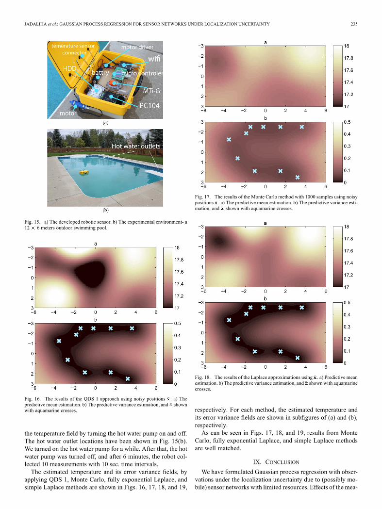
Fig. 17. The results of the Monte Carlo method with 1000 samples using noisypositions . a) The predictive mean estimation. b) The predictive variance esti-mation, and shown with aquamarine crosses.

Fig. 18. The results of the Laplace approximations using . a) Predictive meanestimation. b) The predictive variance estimation, and shownwith aquamarinecrosses.

respectively. For each method, the estimated temperature andits error variance fields are shown in subfigures of (a) and (b),respectively.As can be seen in Figs. 17, 18, and 19, results from Monte

Carlo, fully exponential Laplace, and simple Laplace methodsare well matched.

IX. CONCLUSION

We have formulated Gaussian process regression with obser-vations under the localization uncertainty due to (possibly mo-bile) sensor networks with limited resources. Effects of the mea-


Fig. 19. The results of the simple Laplace method using noise augmented po-sitions shown with aquamarine crosses. a) The predictive mean estimation.b) The predictive variance estimation and shown with aquamarine crosses.

surements noise, localization uncertainty, and prior distributionshave been all correctly incorporated in the posterior predictivestatistics in a Bayesian approach. We have reviewed the MonteCarlo sampling and Laplace’s method, which have been appliedto compute the analytically intractable posterior predictive sta-tistics of the Gaussian processes with localization uncertainty.The approximation error and complexity of all the proposed ap-proaches have been analyzed. In particular, we have providedtradeoffs between the error and complexity of Laplace approx-imations and their different degrees such that one can choose atradeoff taking into account the performance requirements andcomputation complexity due to the resource-constrained sensornetwork. Simulation study demonstrated that the proposed ap-proaches perform much better than approaches without con-sidering the localization uncertainty properly. Finally, we ap-plied the proposed approaches on the experimentally collectedreal data to provide proof of concept tests and evaluation ofthe proposed schemes in practice. From both simulation andexperimental results, the proposed methods outperformed thequick-and-dirty solutions often used in practice.

APPENDIX

A. Regularity Conditions

In this section, we review a set of regularity conditions [26].Let denote the open ball of radius centered at , i.e.,

. Let be the asymptoticmode of order . The followings are regularity conditions.

A.1 .A.2 .A.3 , for all and all

with , where .A.4 is positive definite and

.

A.5 and

where .

REFERENCES[1] D. Culler, D. Estrin, and M. Srivastava, “Guest editors’ introduction:

Overview of sensor networks,” Computer, vol. 37, no. 8, pp. 41–49,Aug. 2004.

[2] D. Estrin, D. Culler, K. Pister, and G. Sukhatme, “Connecting the phys-ical world with pervasive networks,” Pervasive Comput., vol. 1, no. 1,pp. 59–69, 2002.

[3] K. M. Lynch, I. B. Schwartz, P. Yang, and R. A. Freeman, “Decentral-ized environmental modeling bymobile sensor networks,” IEEE Trans.Robot., vol. 24, no. 3, pp. 710–724, Jun. 2008.

[4] J. Choi, S. Oh, and R. Horowitz, “Distributed learning and cooperativecontrol for multi-agent systems,” Automatica, vol. 45, pp. 2802–2814,2009.

[5] J. Cortés, “Distributed Kriged Kalman filter for spatial estimation,”IEEE Trans. Autom. Control, vol. 54, no. 12, pp. 2816–2827, 2010.

[6] N. Cressie, “Kriging nonstationary data,” J. Amer. Statist. Assoc., vol.81, no. 395, pp. 625–634, 1986.

[7] C. E. Rasmussen and C. K. I. Williams, Gaussian Processes for Ma-chine Learning. Cambridge, MA: MIT Press, 2006.

[8] A. Krause, C. Guestrin, A. Gupta, and J. Kleinberg, “Near-optimalsensor placements: Maximizing information while minimizing com-munication cost,” in Proc. ACM 5th Int. Conf. Inf. Process. SensorNetw., 2006, pp. 2–10.

[9] A. Krause, A. Singh, and C. Guestrin, “Near-optimal sensor place-ments in Gaussian processes: Theory, efficient algorithms and empir-ical studies,” J. Mach. Learn. Res., vol. 9, pp. 235–284, 2008.

[10] Y. Xu, J. Choi, and S. Oh, “Mobile sensor network coordination usingGaussian processes with truncated observations,” IEEE Trans. Robot.,vol. 27, no. 6, pp. 1118–1131, 2011.

[11] K. Ho, “Alleviating sensor position error in source localization usingcalibration emitters at inaccurate locations,” IEEE Trans. Signal Pro-cesd., vol. 58, no. 1, pp. 67–83, 2010.

[12] L. Hu and D. Evans, “Localization for mobile sensor networks,” inProc. ACM 10th Annu. Int. Conf. Mobile Comput. Netw., 2004, pp.45–57.

[13] P. Oguz-Ekim, J. Gomes, J. Xavier, and P. Oliveira, “Robust local-ization of nodes and time-recursive tracking in sensor networks usingnoisy range measurements,” IEEE Trans. Signal Process., vol. 59, no.8, pp. 3930–3942, 2011.

[14] R. Karlsson and F. Gustafsson, “Bayesian surface and underwater nav-igation,” IEEE Trans. Signal Process., vol. 54, no. 11, pp. 4204–4213,2006.

[15] D. Titterton and J. Weston, Strapdown Inertial Navigation Tech-nology. Stevenage, U.K.: Peregrinus, 2004.

[16] Y. Xu and J. Choi, “Adaptive sampling for learning Gaussian processesusing mobile sensor networks,” Sensors, vol. 11, no. 3, pp. 3051–3066,2011.

[17] M. Mysorewala, D. Popa, and F. Lewis, “Multi-scale adaptive sam-pling with mobile agents for mapping of forest fires,” J. Intell. Robot.Syst., vol. 54, no. 4, pp. 535–565, 2009.

[18] A. Girard, C. Rasmussen, J. Candela, and R. Murray-Smith, “Gaussianprocess priors with uncertain inputs-application to multiple-step aheadtime series forecasting,” Adv. Neural Inf. Process. Syst., pp. 545–552,2003.

[19] J. Kocijan, R. Murray-Smith, C. Rasmussen, and B. Likar, “Predic-tive control with Gaussian process models,” inProc. IEEEEUROCON,2003, vol. 1, pp. 352–356.

[20] R. Murray-Smith, D. Sbarbaro, C. Rasmussen, and A. Girard, “Adap-tive, cautious, predictive control with Gaussian process priors,” inProc. 13th IFAC Symp. Syst. Identification, Rotterdam, The Nether-lands, 2003, pp. 1195–1200.

[21] M. Deisenroth, C. Rasmussen, and J. Peters, “Gaussian process dy-namic programming,” Neurocomput., vol. 72, no. 7–9, pp. 1508–1524,2009.

[22] D. Nash and M. Hannah, “Using Monte-Carlo simulations andBayesian Networks to quantify and demonstrate the impact of fer-tiliser best management practices,” Environ. Modelling Softw., vol.26, no. 9, pp. 1079–1088, 2011.

[23] M. Wainwright and M. Jordan, “Graphical models, exponential fam-ilies, and variational inference,” Found. Trends Mach. Learn., vol. 1,no. 1–2, pp. 1–305, 2008.


[24] L. Tierney and J. Kadane, “Accurate approximations for posterior mo-ments andmarginal densities,” J. Amer. Statist. Assoc., vol. 81, no. 393,pp. 82–86, 1986.

[25] L. Tierney, R. Kass, and J. Kadane, “Fully exponential Laplace ap-proximations to expectations and variances of nonpositive functions,”J. Amer. Statist. Assoc., vol. 84, no. 407, pp. 710–716, 1989.

[26] Y. Miyata, “Fully exponential Laplace approximations using asymp-totic modes,” J. Amer. Statist. Assoc., vol. 99, no. 468, pp. 1037–1049,2004.

[27] Y. Miyata, “Laplace approximations to means and variances withasymptotic modes,” J. Statist. Planning Inference, vol. 140, no. 2, pp.382–392, 2010.

[28] M. Jadaliha, Y. Xu, and J. Choi, “Gaussian process regression usingLaplace approximations under localization uncertainty,” in Proc.Amer. Control Conf., Montreal, QC, Canada, Jun. 27–29, 2012, pp.1394–1399.

[29] A. J. Smola and P. L. Bartlett, “Sparse greedy Gaussian process re-gression,” in Proc. Adv. Neural Inf. Process. Syst., 2001, vol. 13, pp.619–625.

[30] C. Williams and M. Seeger, “Using the Nystrom method to speed upkernel machines,” in Proc. Adv. Neural Inf. Process. Syst., 2001, vol.13, pp. 682–688.

[31] N. Lawrence, M. Seeger, and R. Herbrich, “Fast sparse Gaussianprocess methods: The informative vector machine,” in Proc. Adv.Neural Inf. Process. Syst., 2003, pp. 625–632.

[32] M. Seeger, “Bayesian Gaussian process models: PAC-Bayesian gener-alisation error bounds and sparse approximations,” Ph.D. dissertation,School of Informatics, Univ. of Edinburgh, Edinburgh, U.K., 2003.

[33] V. Tresp, “A Bayesian committee machine,” Neural Comput., vol. 12,no. 11, pp. 2719–2741, 2000.

[34] A. Brix and P. Diggle, “Spatiotemporal prediction for log-GaussianCox processes,” J. Roy. Statist. Soc.: Series B (Statist. Methodol.), vol.63, no. 4, pp. 823–841, 2001.

[35] C. Andrieu, N. De Freitas, A. Doucet, and M. Jordan, “An introductionto MCMC for machine learning,” Mach. Learn., vol. 50, no. 1, pp.5–43, 2003.

[36] J. Geweke, “Bayesian inference in econometric models using MonteCarlo integration,” Econometrica: J. Econometric Soc., vol. 57, no. 6,pp. 1317–1339, 1989.

[37] H. Durrant-Whyte and T. Bailey, “Simultaneous localisation and map-ping (SLAM): Part I the essential algorithms,” Robot. Autom. Mag.,vol. 13, no. 2, pp. 99–110, 2006.

[38] N. Johnson, S. Yun, H. Thompson, C. Brant, and W. Li, “A synthe-sized pheromone induces upstream movement in female sea lampreyand summons them into traps,” Proc. Nat. Acad. Sci., vol. 106, no. 4,p. 1021, 2009.

[39] B. Smith and J. Tibbles, “Sea lamprey (petromyzon marinus) inlakes huron, michigan, and superior: History of invasion and con-trol, 1936–78,” Can. J. Fisheries Aquatic Sci., vol. 37, no. 11, pp.1780–1801, 1980.

[40] G. Christie and C. Goddard, “Sea lamprey international symposium(slis ii): Advances in the integrated management of sea lamprey in thegreat lakes,” J. Great Lakes Res., vol. 29, pp. 1–14, 2003.

[41] N. Johnson, M. Luehring, M. Siefkes, and W. Li, “Mating pheromonereception and induced behavior in ovulating female sea lampreys,” N.Amer. J. Fisheries Manage., vol. 26, no. 1, pp. 88–96, 2006.

[42] Xsens Company, MTi-G, Miniature AHRS With Integreted GPS,2009 [Online]. Available: http://www.xsens.com/images/stories/prod-ucts/PDF_Brochures/mti-g leaflet.pdf

[43] M. Jadaliha and J. Choi, “Environmental monitoring using au-tonomous aquatic robots: Sampling algorithms and experi-ments,” IEEE Trans. Control Syst. Technol., 2012, Preprint, DOI:10.1109/TCST.2012.2190070.

Mahdi Jadaliha received the B.S. degree in elec-trical engineering from Iran University of Scienceand Technology, Tehran, Iran, in 2005 and theM.S. degree in electrical engineering from SharifUniversity of Technology, Tehran, Iran, in 2007.Currently, he is working toward the Ph.D. degree

in mechanical engineering at Michigan State Uni-versity, East Lansing, under the guidance of Prof.J. Choi. His research interests include statisticallearning and system identification, with applicationsto mobile robotic sensors and SLAM.

Mr. Jadaliha’s paper was a finalist for the Best Student Paper Award at theDynamic System and Control Conference (DSCC) 2012.

Yunfei Xu received the B.S. and M.S. degrees inautomotive engineering from Tsinghua University,Beijing, China, in 2004 and 2007, respectively, andthe Ph.D. degree in mechanical engineering fromMichigan State University, East Lansing, in 2011.Currently, he is a Postdoctoral Researcher in the

Department of Mechanical Engineering at MichiganState University. His current research interestsinclude environmental adaptive sampling algo-rithms, Gaussian processes, and statistical learningalgorithms with applications to robotics and mobile

sensor networks.

Jongeun Choi received the B.S. degree in mechan-ical design and production engineering from YonseiUniversity, Seoul, Republic of Korea, in 1998 and theM.S. and Ph.D. degrees in mechanical engineeringfrom the University of California at Berkeley in 2002and 2006, respectively.He is currently an Associate Professor with the

Department of Mechanical Engineering and theDepartment of Electrical and Computer Engineeringat Michigan State University. East Lansing. His re-search interests include systems and control, system

identification, and Bayesian inference, with applications to mobile robots,environmental adaptive sampling, engine control, and biomedical problems.Dr. Choi was a recipient of an NSF CAREERAward in 2009. His papers were

finalists for the Best Student Paper Award at the Twenty-Fourth American Con-trol Conference (ACC) 2005 and the Dynamic System and Control Conference(DSCC) 2011 and 2012. He is a member of ASME.

Nicholas S. Johnson received the B.S. degree in fish-eries/limnology and biology from the University ofWisconsin, Stevens Point, in 2004 and the M.S. andPh.D. degrees in fisheries and wildlife fromMichiganState University, East Lansing, in 2005 and 2008, re-spectively.He is currently a Research Ecologist with the

United States Geological Survey, Great Lakes Sci-ence Center, Hammond Bay Biological Station, andAdjunct Assistant Professor in the Department ofFisheries and Wildlife at Michigan State University.

His research interests include behavioral and chemical ecology of fishes andspecifically how to use chemical and electrical stimuli to aid restoration ofvalued fishes and control of invasive fishes.

Weiming Li received the B.S. degree in aquacul-ture and the M.S. degree in fish physiology fromShanghai Ocean University, Shanghai, China, in1982 and 1987, respectively, and the Ph.D. degree infisheries from the University of Minnesota at TwinCities in 1994.He is a Professor and FEJ Fry Chair in Environ-

mental Physiology in the Departments of Fisheriesand Wildlife and of Physiology at Michigan StateUniversity, East Lansing, where he is also a facultymember of the Neuroscience Program and the

Ecology, Evolutionary Biology and Behavior Program. His research interestsinclude chemical ecology, physiology of olfaction and endocrine systems, andgenomics.

IEEE TRANSACTIONS ON SIGNAL PROCESSING, …jchoi/files/papers/JXCJW_TSP2013.pdfimation techniques...

Documents

Transcript of IEEE TRANSACTIONS ON SIGNAL PROCESSING, …jchoi/files/papers/JXCJW_TSP2013.pdfimation techniques...