IEEE TRANSACTIONS ON RADIATION AND PLASMA MEDICAL SCIENCES, VOL. 1, NO. 6, NOVEMBER 2017 517

Calibration for Circular Cone-Beam CTBased on Consistency Conditions

Jérôme Lesaint, Simon Rit, Rolf Clackdoyle, and Laurent Desbat

Abstract—In cone-beam computed tomography (CT), impre-cise knowledge of the acquisition geometry can severely impactthe quality of the reconstructed image. This paper investigatesgeometric calibration using data consistency conditions (DCCs).Unlike the usual marker-based off-line methods, the proposedmethod does not require the extra-scan of a calibration phantom.It is based on the minimization of a cost function, which mea-sures the inconsistency between pairs of projections. The methodhas been applied to both simulated and real data. The latter wereacquired from a micro-CT system with circular trajectory, forwhich the problem reduces to identifying global misalignmentsof the system. When compared to uncorrected reconstruction,the method significantly improved the image quality. When com-pared to marker-based calibration method, the image quality wassimilar but no calibration scan was required. Finally, the methodcan handle axially truncated data. Axial truncation is very com-mon in the medical context but often considered intractable forDCC-based methods. We also demonstrate DCC calibration fromreal data with axial truncation.

Index Terms—Cone-beam computed tomography (CBCT),data consistency conditions (DCCs), geometric calibration,micro-CT.

I. INTRODUCTION

IN CONE-BEAM computed tomography (CBCT), a 3-Dimage is reconstructed from a set of 2-D projections

acquired from a point-like X-ray source. Poor reconstructedimage quality can arise due to many possible causes. Oneof these causes is an inaccurate calibration of the system.Calibration is the process through which the geometry ofacquisition of the projections is accurately determined. Bygeometry of acquisition, we mean the position and orienta-tion of the detector and the position of the X-ray source in afixed reference frame.

Calibration of a CBCT system has been studied for a longtime. Early works used the scan of a dedicated phantom to

Manuscript received April 18, 2017; revised July 4, 2017; acceptedJuly 28, 2017. Date of publication August 1, 2017; date of current versionNovember 1, 2017. This work was supported by the Agence Nationale dela Recherche, France, under Grant Labex CAMI ANR-11-LABX-0004-01,Grant Labex PRIMES ANR-11-LABX-0063, and Project DROITE ANR-12-BS01-0018. (Corresponding author: Jérôme Lesaint.)

J. Lesaint, R. Clackdoyle, and L. Desbat are with the TIMC-IMAGLaboratory, CNRS UMR 5525, Université Grenoble Alpes, 38707 La Tronche,France (e-mail: jerome.lesaint@univ-grenoble-alpes.fr).

S. Rit is with Univ. Lyon, INSA-Lyon, UCB Lyon 1, UJM-Saint Etienne,CNRS, Inserm, CREATIS UMR5220, U1206, Centre Léon Bérard, F-69373Lyon, France.

Color versions of one or more of the figures in this paper are availableonline at http://ieeexplore.ieee.org.

Digital Object Identifier 10.1109/TRPMS.2017.2734844

estimate the geometric parameters. These are known as off-line methods, to emphasize the need for a preliminary scan.The calibration scan provides accurate geometry informationas long as the misalignments that were estimated are repro-ducible over time. In the extreme case, where mechanicalflexibility of the system makes the reproducibility assump-tion false, these methods become invalid. More recently,on-line (or self-) calibration methods have been developed. Foreach acquisition, and before reconstruction, the calibration iscomputed directly from the projections.

This paper presents an on-line method based on theminimization of a cost function, that quantifies the incon-sistency of the set of measured projections. The data con-sistency conditions (DCCs) that are incorporated in the costfunction have been described in many different works (seeSection II-C). They are essentially fan-beam consistency con-ditions for a linear trajectory. They have been adapted to acircular trajectory CBCT system by resampling each pair ofprojections into a virtual detector parallel to the line connect-ing pairs of source positions. This idea was already proposedin [1] but, to the best of our knowledge, never implemented orapplied to any CT reconstruction problem. This paper is verysimilar in its geometric approach to other recent works [2], [3]but differs fundamentally in the DCCs which are used. Theproposed method was applied to simulated and real data, andcompared with a robust off-line method.

II. NOTATION AND BACKGROUND

The micro-CT system to which the calibration method wasapplied is made of a 2-D flat detector and a fixed X-ray source.A turntable placed between the two allowed a full 360◦ rota-tion of the object (see Fig. 1), so the acquisition geometry wasequivalent to a circular trajectory of the source and detector.We will describe the geometry in detail, together with thecalibration parameters that we are trying to estimate.

A. Description of the Geometry

We use the same geometric description as that given in [4].The detector cells are perfect squares (same width and height,arranged on a Cartesian grid). Let (x, y, z) be a fixed ref-erence frame, defined as follows: the y-axis is the axis ofrotation of the turntable. The origin is set so that the sourcelies in the y = 0 plane. The z-axis contains the source at rota-tion angle 0 and points in the direction of the source. Thex-axis is defined so that (x, y, z) is a right-handed coordi-nate system. The flat panel detector is equipped with a direct

2469-7311 c© 2017 IEEE. Personal use is permitted, but republication/redistribution requires IEEE permission.See http://www.ieee.org/publications_standards/publications/rights/index.html for more information.

518 IEEE TRANSACTIONS ON RADIATION AND PLASMA MEDICAL SCIENCES, VOL. 1, NO. 6, NOVEMBER 2017

Fig. 1. Picture of the CT system. Source (left) is fixed. Turntable (middle)and detector (right) are adjustable. Detector size: 35 × 35 mm. Pixel size:17.09 μm.

Fig. 2. Illustration of the eight geometric parameters. The detector orientationis defined by three Euler angles. η is the in-plane angle. φ and θ are out-of-plane rotations about the v-axis and the u-axis, respectively.

(u, v) coordinate system whose origin is the center of thedetector and whose axes coincide with the pixel rows andcolumns, respectively. The geometry of one projection can beunambiguously described with eight parameters (see Fig. 2).

• The rotation angle λ, taken from the z-axis.• The radius of the source trajectory R.• Three orientation angles of the detector (φ, θ, η).• The source to detector distance D (or focal distance).• The coordinates (u0, v0) of the principal point (orthogonal

projection of the source onto the detector plane).With this parametrization, for λ ∈ [0; 2π [, the source posi-

tion is given by �sλ = (R sin λ, 0, R cos λ). The orientation ofthe detector is described with three Euler angles η, θ , andφ (called yaw, pitch, roll, respectively, in [5] and skew, tilt,slant in [6]) applied in this order (respective axes of rota-tions are illustrated in Fig. 2). The normal to the detectoris defined with two out-of-plane angles θ and φ about the u-and v-axes, respectively. The in-plane rotation (about the focalaxis) is given by η. The circular geometry thus consists of 8degrees-of-freedom, unless the relative position and orientation

Fig. 3. Cone-beam geometry with circular trajectory. For a given scalar λ

(typically in [0, 2π ]), �sλ denotes the position of the source. �α is a unit 3-Dvector (∈ S2) that gives the direction of one X-ray. Note here that the systemis perfectly aligned: the v-axis is parallel to the rotation y-axis (θ = η = 0).The u-axis is perpendicular to the direction of the source (φ = 0) and thedetector is not shifted (u0 = v0 = 0).

of the source and detector can vary across projections. In ourmicro-CT system, the source and the detector are fixed, so theonly projection-specific parameter is the rotation angle. Theother seven parameters remain constant through the acqui-sition cycle. We call these parameters global misalignmentparameters or global geometric parameters and refer to thecorresponding geometry as true geometry. The system is per-fectly aligned when (1) the principal axis (orthogonal to thedetector plane and passing through the source) contains boththe world origin and the detector origin and (2) the u andv axes of the detector are parallel to the x and y axes ofthe world frame at rotation angle λ = 0. In terms of thegeometric parameters, these two conditions are equivalent toθ = φ = η = u0 = v0 = 0. We refer to the correspondinggeometry as nominal geometry.

B. X-Ray Line-Integral Model

If f (�x) = f (x, y, z) denotes the object density function, theprojection g(λ, ·) is defined by the usual line integral model

g(λ, �α) =∫ ∞

0f (�sλ + t�α)dt, ∀�α ∈ S2 (1)

where S2 denotes the unit-sphere of R3. The projection g(λ, ·)

vanishes for all �α such that the line originating at �sλ anddirected by �α does not intersect the support of f (see Fig. 3).

C. Review of Existing Calibration Methods

Much work has been done on the calibration of CT systems.We give a quick review of the methods and briefly summa-rize the relative importance of each parameter with respectto their impact on the reconstruction quality. If N denotesthe number of acquired projections, the most general calibra-tion problem consists of estimating—for each projection—theeleven independent coefficients of the 3 × 4 projection matrix

LESAINT et al.: CALIBRATION FOR CIRCULAR CBCT BASED ON CONSISTENCY CONDITIONS 519

in homogeneous coordinates (see [7]). If the detector rows andcolumns are known to be perpendicular with the same sam-pling in both directions (i.e., square pixels) then two degreesof freedom are eliminated and the task reduces to estimatingnine projection-specific geometric parameters (three for thesource position, three for the detector position, and anotherthree for the orientation of the gantry). As described in theprevious section, the circular trajectory we are considering inthis paper is completely described by seven global geomet-ric parameters. The only projection-specific parameter is therotation angle.

Imaging-based calibration methods fall into two broadcategories. One category consists of the off-line meth-ods [4]–[6], [8]–[12]: they all require prescanning of acalibration phantom, usually made up of small ball bear-ings (BBs) whose relative positions are accurately known.Then the theoretical projections of the BBs (which dependon the geometric parameters) are compared with theiractual projections to derive—iteratively [8], [9] or analyti-cally [4]–[6], [10]–[12]—the calibration parameters. In [12],they solve the complete calibration problem and analyticallyderive all nine parameters for each projection.

The other group of techniques consists of on-line tech-niques. All methods in this category solve the calibrationproblem without a specific calibration scan of a calibra-tion object. They only use the data from the projections ofthe imaged object. Beyond this common feature, this groupencompasses substantially different techniques. In [13]–[15],they minimize a cost function, whose evaluation requires thereconstruction of the object from the current estimate of thegeometric parameters. The metric is based on entropy in [13],the L2-norm of the image gradient in [14] or the mutual infor-mation between reprojected image and projection data in [15].The limitation of such methods is the computational load,which may not fit clinical workflow (though [14] limits thisdrawback by only reconstructing a fraction of the volume).In [16], they use the 3-D reconstruction of a planning CTand compute projection-specific geometric parameters by reg-istering the actual projections with the reprojected CT image.Other works in this category utilize the redundancy of theprojection data (i.e., the DCCs). In the 2-D parallel beamcase, Basu and Bresler [17], [18] solved uniquely and effi-ciently the problem of unknown projection angles and shiftswith the Helgason–Ludwig DCCs. Some works use the trivial“opposite-ray” condition [19]–[21]. In [19], this DCC, whichnormally only applies in the central plane (the plane of thetrajectory), is extended to cone-beam projections of a par-ticular class of symmetric 3-D object functions and showsaccurate calibration results when approximated in a centralregion of a generic object. More closely related to this paperis a series of publications on epipolar consistency condi-tions (ECCs) [2], [3], [22]. These DCCs are based on theGrangeat theorem and relate the derivative of the 2-D Radontransform of the projections to the derivative of the 3-D Radontransform of the imaged object.

The comparison of previous works is not easy due to theparametrization which may differ with authors. Nevertheless, itis widely documented that the detector shift u0 and the in-plane

angle η are of crucial importance [4]–[6], [11]. On the otherhand, [11], [15] demonstrated that the two out-of-plane angles(φ and θ ) may be set to zero without affecting the image qual-ity if their true values are kept below 2◦ (which is a reasonablemanufacturing accuracy requirement). Finally, miscalibrationof the source-to-center and source-to-detector distances doesnot introduce artifacts in the reconstructed volume and aretherefore not calibrated. However, these two parameters affectthe magnification of the reconstructed volume, which wouldnot be acceptable in some cases, such as a metrology-orientedapplication.

III. METHODS

A. Cone-Beam DCCs for Linear Trajectory

DCCs are conditions which must be satisfied by the pro-jection data in order for them to be the image of an objectfunction through the forward projection model describedin (1). DCCs have been applied to various CT artefact cor-rection techniques, e.g., motion compensation [23]–[25] andbeam hardening correction [26]. The simplest condition isthe “opposite-ray condition.” In parallel projection geome-try, it states that the projections must be even: Rf (�α, s) =Rf (−�α,−s), where Rf denotes the 2-D Radon transform ofan object function f . This condition was applied to the cali-bration problem in [19]. Still in the parallel geometry, thereexists a complete set of DCCs, known as Helgason–LudwigDCCs (see [27], [28] and standard textbooks on the Radontransform, e.g., [29] and [30]), which relates the nth ordermoments of each projection to a homogeneous polynomial oforder n. In the 2-D divergent geometry (fan-beam projections),complete DCCs, similar to Helgason–Ludwig polynomial con-ditions, were derived in [31] for the particular case of an X-raysource moving along a line. We will be using the order-0 case,which was known much earlier than the latter work (see theirvarious guises in [32]–[36] for a review).

The description of cone-beam pair-wise consistency condi-tions follows [1]. Let �sλi and �sλj be two source positions andLi,j be the line connecting them. Suppose that both projectionsare acquired with one common flat detector, parallel to Li,j.Any plane containing Li,j intersects—if it does—the detectoron a row, parallel to Li,j, which we will index with k. We willdenote that plane Pi,j,k. The situation in Pi,j,k reduces to apair of fan-beam projections along the virtual linear trajectoryLi,j and with the kth detector row playing the role of the 1-Dfan-beam detector. The order-0 DCCs state the following.

Lemma 1: For any pair of projection indices i, j and anyinteger k, let

Gi,j,k =∫ π

2

− π2

g(λi, �αk

φ

)

cos φdφ (2)

where �αkφ denotes a unit vector in Pi,j,k, φ denotes the

angle between �αkφ and the perpendicular to Li,j in that plane.

Furthermore, the line Li,j is assumed to not intersect thesupport of the object function f . See Figs. 4 and 5.

If the data are consistent, then

Gi,j,k − Gj,i,k = 0 (3)

520 IEEE TRANSACTIONS ON RADIATION AND PLASMA MEDICAL SCIENCES, VOL. 1, NO. 6, NOVEMBER 2017

Fig. 4. View of one plane Pi,j,k . Order-0 fan-beam DCCs state that theintegral of the cosine-weighted projections are equal.

Fig. 5. Two sources on a circular trajectory. Both projections are backpro-jected in a virtual detector, parallel to the line connecting �sλi and �sλj .

Let ci,j,k denote the square difference of the left-hand sideof (3). The sum Ci,j = ∑

k ci,j,k is a measure of the pair-wiseconsistency between two cone-beam projections g(λi, ·) andg(λj, ·).

B. Resampling in Virtual Detector

These DCCs only apply if the detector is parallel to thevirtual linear trajectory Li,j connecting two source positions.In the circular trajectory we are considering in this paper, thisdetector condition is obviously not fulfilled. To remedy thisproblem, each pair of projections is resampled onto a virtualdetector Vi,j by means of a backprojection. The virtual detectoris placed at the origin of the world system of coordinatesand oriented in such a way that the rows and columns of Vi,j

are parallel to Li,j and the axis of rotation, respectively. Thesituation is illustrated in Fig. 5.

The orientation of the virtual detector allows a simple eval-uation of the integral Gi,j,k in (2) by changing the φ-variableto the u-pixel coordinate of the virtual detector with

u =√

v2k + D2

virt tan φ

Algorithm 1 Pseudo-Code for the Cost Function1: procedure COST(p)2: Initalize C = 03: for Each pair of sources (i, j) ∈ �: do4: Backproject projections onto Vi,j.5: Pre-weight the virtual projections acc. to Eq. 4.6: for Each row k: do7: Compute the line integrals Gi,j,k and Gj,i,k.8: Compute the squared difference ci,j,k.9: Add to C.

10: end for11: end for12: end procedure

where vk is the intercept of the plane Pi,j,k with the vir-tual detector’s v-axis and Dvirt denotes the distance from thesource to the virtual detector. Applying this change of variablesleads to

Gi,j,k = 1√v2

k + D2virt

∫R

g(λi, u)

√v2

k + D2virt√

u2 + v2k + D2

du. (4)

Note that the weight inside the integral is exactly cos φ.The change of variables has moved this cosine term from thedenominator to the numerator.

When applying these DCCs to the calibration problem, wenote that the backprojection onto the virtual detector will usethe projection geometry as input. Hence, the dependency of thecost function (described in the next section) on the calibrationparameters via this backprojection.

C. Consistency Metric

Estimation of the geometric calibration parameters isachieved by minimizing a cost function based on the pair-wise consistency conditions described above. Let p =(φ, θ, η, u0, v0, R, D) denote the 7-uple of sought parameters.We define the cost function C(p) as follows:

C(p) =∑

(i,j)∈�

Ci,j =∑

(i,j)∈�

∑k

ci,j,k (5)

where Ci,j was defined above with the dependence on p buriedin the backprojection onto the virtual detector, � is the chosensubset of pairs of projections to which the DCCs are applied.

The size of the virtual detector Vi,j is computed to accountfor the distortion resulting from the backprojection step (seedetails is Section V-C1). For each pair of projections, the costfunction is evaluated over all rows k of Vi,j.

The computation of the cost function can be summarized inAlgorithm 1.

IV. NUMERICAL EXPERIMENTS ON SIMULATED DATA

We first studied the properties of our cost function on sim-ulated projections of a Shepp–Logan phantom and estimatedthe accuracy that can be expected from our method. All sim-ulated projection data were generated with the reconstruction

LESAINT et al.: CALIBRATION FOR CIRCULAR CBCT BASED ON CONSISTENCY CONDITIONS 521

Fig. 6. Cost function as a 1-D function of each estimated parameter, eval-uated on the simulated projection data of a standard Shepp–Logan phantom.90 equally spaced projections were simulated over a full 360◦ circular acqui-sition. For each parameter, the cost function is evaluated at 50 equally-spacedparameter values, ranging from −2 to 2. Note that the minimum functionvalue is not zero due to numerical errors.

toolkit (RTK) software package [37]. All reconstructions werecomputed with the Feldkamp algorithm [38] available in RTK.

In all our experiments, the set � was composed of 27projections pairs, constructed as follows: nine equally spacedprojections (spaced by 40◦) were selected and all possible pairswere included in �, except those separated by ±160◦. Thisparticular choice for � arose from a tradeoff between the com-putational load and the amount of data we inject in the costfunction for robust parameter estimation. Pairs separated by±160◦ were removed because they are too close to the limitsituation where the line Li,j (hence the virtual detector) wouldbe perpendicular to the physical detectors. Also, the maximumseparation of the remaining pairs was 120◦ which eliminatedany risk of the connecting line intersecting the scanned object.

A. Cost Function Study

We first studied the behavior of our cost function on thesimulated projections of a 3-D Shepp–Logan phantom [39].Projections were simulated with a perfectly aligned system(R = 100, D = 200 and all other geometric parameters set tozero). Then, we computed the cost function as a 1-D-functionof each separate parameter, over a symmetric interval [−2, 2](in degrees for η, θ , and φ and in millimeters for u0, v0,R, and D). Fig. 6 shows corresponding plots. Note that thecost function has very low dependence on the two distancesR and D. For this reason, these two parameters will not beoptimized in our calibration method. Our procedure focuseson the remaining five global parameters. The plots in Fig. 6indicate that the cost function is locally convex with respectto each of them. The convexity of the 1-D-functions does notguarantee the convexity of the multidimensional cost functionbut is still encouraging for the optimization procedure to finda suitable minimum. Of the five parameters, the vertical shiftv0 shows the least sensitivity to the DCCs. This fact has a

TABLE IRESULTS ON SIMULATED DATA

direct effect on the errors we obtained with simulated data(see section below).

B. Calibration on Simulated Data

We applied our calibration method to simulated projectionsof a 3-D Shepp–Logan phantom. The data were generatedusing the misalignment parameter values indicated in the firstrow of Table I. The simulated projections were 256 × 256pixels, with pixel size set to 0.25 mm. The source-to-centerand source-to-detector distances were set to 100 and 160 mm,respectively. The larger half-length of the outer ellipsoïd ofthe Shepp–Logan phantom was 15 mm. We used the Numpyimplementation of the order-0 minimization method fromPowell [40]. Results are recorded in Table I.

In the first experiment (see Exp. 1 in Table I), the calibra-tion procedure was initialized with a nominal geometry (allfive parameters equal to 0). This initialization corresponds tothe best guess we could make on the real μCT system, whichis designed to be perfectly aligned. In Fig. 7, we present onefrontal slice of the 3-D numerical Shepp–Logan phantom (topleft). We reconstructed the 3-D volume from the simulatedprojections data using three different geometries: 1) the truegeometry; 2) the DCC-calibrated geometry (resulting from ourminimization procedure); and 3) the nominal geometry. Thereconstructions are shown in Fig. 7. The reconstruction withthe nominal geometry shows severe artifacts (see middle leftin Fig. 7) with a root mean square error (RMSE) of 0.311when compared to the 3-D numerical phantom (top left). Novisible difference between the two reconstructions with thetrue geometry (top right) and with DCC-calibrated geometry(middle right) is apparent. In both cases, the quality of thereconstruction is significantly improved, with RMSE of 0.107and 0.106, respectively. Note also that the procedure can eas-ily be extended to a short scan trajectory. In the bottom rowof Fig. 7, we present a 220◦ short-scan reconstructions withthe nominal geometry (left) and the DCC-calibrated geom-etry (right). The set � was built with nine equally spacedprojections over the 220◦ angular range.

The second experiment focuses on the dependency of thecost function on the initial guess. We ran the procedure with100 random initial values taken from a normal distribution andcomputed the mean and standard deviation of each geometric

522 IEEE TRANSACTIONS ON RADIATION AND PLASMA MEDICAL SCIENCES, VOL. 1, NO. 6, NOVEMBER 2017

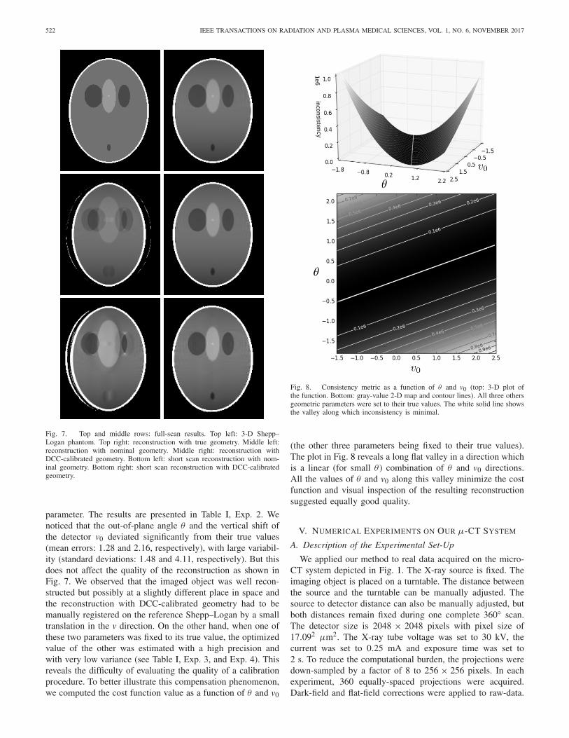
Fig. 7. Top and middle rows: full-scan results. Top left: 3-D Shepp–Logan phantom. Top right: reconstruction with true geometry. Middle left:reconstruction with nominal geometry. Middle right: reconstruction withDCC-calibrated geometry. Bottom left: short scan reconstruction with nom-inal geometry. Bottom right: short scan reconstruction with DCC-calibratedgeometry.

parameter. The results are presented in Table I, Exp. 2. Wenoticed that the out-of-plane angle θ and the vertical shift ofthe detector v0 deviated significantly from their true values(mean errors: 1.28 and 2.16, respectively), with large variabil-ity (standard deviations: 1.48 and 4.11, respectively). But thisdoes not affect the quality of the reconstruction as shown inFig. 7. We observed that the imaged object was well recon-structed but possibly at a slightly different place in space andthe reconstruction with DCC-calibrated geometry had to bemanually registered on the reference Shepp–Logan by a smalltranslation in the v direction. On the other hand, when one ofthese two parameters was fixed to its true value, the optimizedvalue of the other was estimated with a high precision andwith very low variance (see Table I, Exp. 3, and Exp. 4). Thisreveals the difficulty of evaluating the quality of a calibrationprocedure. To better illustrate this compensation phenomenon,we computed the cost function value as a function of θ and v0

Fig. 8. Consistency metric as a function of θ and v0 (top: 3-D plot ofthe function. Bottom: gray-value 2-D map and contour lines). All three othersgeometric parameters were set to their true values. The white solid line showsthe valley along which inconsistency is minimal.

(the other three parameters being fixed to their true values).The plot in Fig. 8 reveals a long flat valley in a direction whichis a linear (for small θ ) combination of θ and v0 directions.All the values of θ and v0 along this valley minimize the costfunction and visual inspection of the resulting reconstructionsuggested equally good quality.

V. NUMERICAL EXPERIMENTS ON OUR μ-CT SYSTEM

A. Description of the Experimental Set-Up

We applied our method to real data acquired on the micro-CT system depicted in Fig. 1. The X-ray source is fixed. Theimaging object is placed on a turntable. The distance betweenthe source and the turntable can be manually adjusted. Thesource to detector distance can also be manually adjusted, butboth distances remain fixed during one complete 360◦ scan.The detector size is 2048 × 2048 pixels with pixel size of17.092 μm2. The X-ray tube voltage was set to 30 kV, thecurrent was set to 0.25 mA and exposure time was set to2 s. To reduce the computational burden, the projections weredown-sampled by a factor of 8 to 256 × 256 pixels. In eachexperiment, 360 equally-spaced projections were acquired.Dark-field and flat-field corrections were applied to raw-data.

LESAINT et al.: CALIBRATION FOR CIRCULAR CBCT BASED ON CONSISTENCY CONDITIONS 523

Fig. 9. Top row: pictures of the imaged objects. Bottom row: one projectionof each object. (a) Glue cap. (b) Concrete sample. (c) Sponge sample.

TABLE IICALIBRATION USING DIFFERENT SUBSETS � OF PROJECTIONS

The negative-log transform was then applied so that the pro-jection data correspond to the line-integral model describedin (1). We report results on three different datasets: the firstone is the projection data of the plastic cap from a tube ofglue, approximately 1 cm wide. The rotating support platformwas in the flat-field images and therefore subtracted from theprojection of the glue-cap. The glue-cap was small enough tobe completely contained in the projections. Consequently, noprojections were truncated. The values of R and D were physi-cally measured to be 219 and 295 mm. The second dataset wasacquired from a sample of concrete foam. All projections weretruncated in the direction of the rotation axis (axial truncation).Measures of R and D were 114 and 137 mm, respectively. Forthis sample, a 0.4 mm aluminum filter was placed in front ofthe X-ray tube to harden the X-ray beam to make the pro-jection data better fit the line integral model. The third dataconsisted in a piece of sponge placed into a plastic syringe.Projections were also axially truncated. Measures of R and Dwere 195 and 259 mm, respectively. See pictures and sampleprojections of the three objects in Fig. 9.

B. Reconstruction With Complete Data

The calibration method was applied to the projectionsacquired from each scan, using the nominal geometry as firstguess. The output values are indicated in Table II. Each of theeight rows in this table corresponds to a different subset of pro-jections, from which the cost function was computed. The first

Fig. 10. Coronal (left) and transverse (right) slices of the reconstructed imagewithout calibration (top row), with DCC-based calibration (second row) andwith marker-based calibration (third row). The intersection of both slices isrepresented by the white line. The corresponding intensity profiles are plottedon the bottom figure.

one was composed of nine equally spaced projections, start-ing with projections at angle 0. Each subsequent subset wasshifted by 5 projections (5◦). Fig. 10 shows coronal and trans-verse slices from the reconstructed images with the nominalgeometry and compares them to reconstructions with a geom-etry estimated using an off-line marker-based method and ourDCC-calibrated geometry. The alignment problem described inSection IV-B was encountered here too and the two calibrated

524 IEEE TRANSACTIONS ON RADIATION AND PLASMA MEDICAL SCIENCES, VOL. 1, NO. 6, NOVEMBER 2017

Fig. 11. Axial truncation management: only those rows between the twodashed lines are retained in the virtual projection.

reconstructions were registered manually in the y direction forcomparison. Note first that subdegree angular misalignmentsand submillimeter detector shifts lead to severe artifacts inthe reconstruction, especially at the edges of the object (seetop-row of Fig. 10). Second, the image quality was signifi-cantly improved when reconstruction was computed with theDCC-calibrated geometry. The edges are sharp as illustratedby the profiles in Fig. 10. Of course, the calibration proceduredoes not correct for other CT artifacts which degrade both un-calibrated and calibrated reconstructed images (e.g., cupping,probably due to beam hardening, and ring artifacts).

C. Reconstruction With Axially Truncated Data

This section explains how our calibration procedure can dealwith axially truncated data with application to the truncateddata acquired on the same μ-CT system (Fig. 9 middle andright).

1) Handling Axial Truncation: Our cost function is the sumof square differences between integral over rows of the virtualdetector. For that reason, truncation in the v-direction doesnot cause any difficulty as long as there is no truncation inthe u-direction. This feature is specific to the nature of theDCCs used in the cost function. In our implementation, caremust be taken at the backprojection level because the squarephysical detector is backprojected to a trapezoidal shape onthe virtual detector, with horizontal pixel rows backprojectedto oblique pixel rows of varying angle (except for the centralline, which remains horizontal). The situation is depicted inFig. 11. The virtual projection can therefore be limited to thosehorizontal rows of the virtual detector that are not truncated(rows between the two dashed lines on Fig. 11 right).

2) Results: The calibration procedure was applied to theconcrete and the sponge datasets. The nominal geometryserved as initial guess. For the concrete sample, the scanningdistances R and D were set to 114 and 137 mm, respec-tively. The resulting cone-angle was approximately 14◦. Forthe sponge sample, R = 195 mm and D = 259 mm.Axial and transverse slices of the reconstructed volumes areshown in Figs. 12 and 13. In the uncalibrated reconstructions,small structures of the object are barely distinguishable. Inthe calibrated reconstruction of the concrete sample, thoughcone-beam and beam-hardening artifacts are still present,

Fig. 12. Concrete sample. Coronal (left) and transverse (right) slices of thereconstructed volume without calibration (top row) and with our DCC-basedcalibration (bottom row).

Fig. 13. Sponge sample. Coronal (left) and transverse (right) slices of thereconstructed volume without calibration (top row) and with our DCC-basedcalibration (bottom row).

the detailed structures (air bubbles in the concrete foam) aremuch more sharply reconstructed.

VI. CONCLUSION

We proposed an on-line calibration method to estimate fivegeometric parameters of a μ-CT system. The method is basedonly on consistency of the “production” scan. It requires noprior (off-line) calibration scan. The quality of the recon-structed images in the experiments compares with the robust

LESAINT et al.: CALIBRATION FOR CIRCULAR CBCT BASED ON CONSISTENCY CONDITIONS 525

“classical” marker-based calibration method. Furthermore, thecalibration method can correctly handle axially-truncated data,which is an untypical feature for DCC-based application.

The design of our cost function can probably be refined.A short study on the individual contribution of a pair of pro-jections revealed that pairs angularly separated by more than90◦ contributed more than close pairs. Hence, a cost functionbuilt from such pairs may convey more independent infor-mation and hence lead to more robust estimation. Anotherquestion is related to the dependency of the cost function onthe object. We have carried out some simulations (similar tothose in Figs. 6 and 8) on objects with sharp edges (a simplex-like simulated object) or plate-like objects (very small extentin the v-direction). In all cases, the cost function behaved simi-larly to the Shepp–Logan study, with regards to each individualparameter or with regards to the (θ, v0) pair. However, thecost function behaved differently when the plate-like objectwas placed in the central plane (containing the source trajec-tory). But, in this case, the geometry collapses to fan-beam,with its own geometric parameters (for example, θ playsno role).

The investigation of the interplay between geometric param-eters is a possible future direction of research. Fig. 8 revealsthat a large error on one parameter can be compensated by alarge error on the second in terms of consistency. We are alsoextending this paper in two directions. The first one appliesthe same principles to estimate projection-specific calibrationparameters, by using a similar cost function for each projec-tion. Second, the comparison of our method with the workin [2], later described as ECCs [3]. ECCs are also applied topairs of projections and use a similar geometry of lines onthe two detectors (as shown in Fig. 5). However, the theoret-ical foundations are different because the ECCs are based onGrangeat’s formula and require the computation of a deriva-tive. Whether these conditions are equivalent to the conditionsused in this paper still needs to be understood and is ongoingwork.

REFERENCES

[1] M. S. Levine, E. Y. Sidky, and X. Pan, “Consistency conditions for cone-beam CT data acquired with a straight-line source trajectory,” TsinghuaSci. Technol., vol. 15, no. 1, pp. 56–61, Feb. 2010. [Online]. Available:http://www.ncbi.nlm.nih.gov/pmc/articles/PMC2886312/

[2] C. Debbeler, N. Maass, M. Elter, F. Dennerlein, and T. M. Buzug,“A new CT rawdata redundancy measure applied to automated misalign-ment correction,” in Proc. 12th Int. Meeting Fully Three DimensionalImage Reconstruct. Radiol. Nucl. Med., 2013, pp. 264–267. [Online].Available: http://www.fully3d.org/2013/Fully3D2013Proceedings.pdf

[3] A. Aichert et al., “Epipolar consistency in transmission imaging,” IEEETrans. Med. Imag., vol. 34, no. 11, pp. 2205–2219, Nov. 2015.

[4] F. Noo, R. Clackdoyle, C. Mennessier, T. A. White, and T. J. Roney,“Analytic method based on identification of ellipse parametersfor scanner calibration in cone-beam tomography,” Phys. Med.Biol., vol. 45, no. 11, pp. 3489–3508, 2000. [Online]. Available:http://stacks.iop.org/0031-9155/45/i=11/a=327

[5] M. J. Daly, J. H. Siewerdsen, Y. B. Cho, D. A. Jaffray, and J. C. Irish,“Geometric calibration of a mobile C-arm for intraoperative cone-beamCT,” Med. Phys., vol. 35, no. 5, pp. 2124–2136, May 2008.

[6] L. von Smekal, M. Kachelriess, E. Stepina, and W. A. Kalender,“Geometric misalignment and calibration in cone-beam tomography,”Med. Phys., vol. 31, no. 12, pp. 3242–3266, Dec. 2004.

[7] R. Hartley and A. Zisserman, Multiple View Geometry in ComputerVision, 2nd ed. Cambridge, U.K.: Cambridge Univ. Press, 2000.

[8] G. T. Gullberg, B. M. Tsui, C. R. Crawford, J. G. Ballard, andJ. T. Hagius, “Estimation of geometrical parameters and collima-tor evaluation for cone beam tomography,” Med. Phys., vol. 17,no. 2, pp. 264–272, 1990. [Online]. Available: http://dx.doi.org/10.1118/1.596505

[9] P. Rizo, P. Grangeat, and R. Guillemaud, “Geometric calibration methodfor multiple-head cone-beam SPECT system,” IEEE Trans. Nucl. Sci.,vol. 41, no. 6, pp. 2748–2757, Dec. 1994.

[10] Y. Cho, D. J. Moseley, J. H. Siewerdsen, and D. A. Jaffray, “Accuratetechnique for complete geometric calibration of cone-beam com-puted tomography systems,” Med. Phys., vol. 32, no. 4, pp. 968–983,Apr. 2005.

[11] K. Yang, A. L. C. Kwan, D. F. Miller, and J. M. Boone, “A geometriccalibration method for cone beam CT systems,” Med. Phys., vol. 33,no. 6, pp. 1695–1706, Jun. 2006.

[12] C. Mennessier, R. Clackdoyle, and F. Noo, “Direct determinationof geometric alignment parameters for cone-beam scanners,” Phys.Med. Biol., vol. 54, no. 6, pp. 1633–1660, 2009. [Online]. Available:http://stacks.iop.org/0031-9155/54/i=6/a=016

[13] Y. Kyriakou, R. M. Lapp, L. Hillebrand, D. Ertel, and W. A. Kalender,“Simultaneous misalignment correction for approximate circular cone-beam computed tomography,” Phys. Med. Biol., vol. 53, no. 22,pp. 6267–6289, Oct. 2008. [Online]. Available: http://dx.doi.org/10.1088/0031-9155/53/22/001

[14] A. Kingston, A. Sakellariou, T. Varslot, G. Myers, and A. Sheppard,“Reliable automatic alignment of tomographic projection data by passiveauto-focus,” Med. Phys., vol. 38, no. 9, pp. 4934–4945, 2011.

[15] J. Muders and J. Hesser, “Stable and robust geometric self-calibrationfor cone-beam CT using mutual information,” IEEE Trans. Nucl. Sci.,vol. 61, no. 1, pp. 202–217, Feb. 2014.

[16] S. Ouadah, J. W. Stayman, G. J. Gang, T. Ehtiati, and J. H. Siewerdsen,“Self-calibration of cone-beam CT geometry using 3D–2D image regis-tration,” Phys. Med. Biol., vol. 61, no. 7, pp. 2613–2632, 2016. [Online].Available: http://stacks.iop.org/0031-9155/61/i=7/a=2613

[17] S. Basu and Y. Bresler, “Uniqueness of tomography with unknown viewangles,” IEEE Trans. Image Process., vol. 9, no. 6, pp. 1094–1106,Jun. 2000.

[18] S. Basu and Y. Bresler, “Feasibility of tomography with unknown viewangles,” IEEE Trans. Image Process., vol. 9, no. 6, pp. 1107–1122,Jun. 2000.

[19] D. Panetta, N. Belcari, A. D. Guerra, and S. Moehrs, “An optimization-based method for geometrical calibration in cone-beam CT without dedi-cated phantoms,” Phys. Med. Biol., vol. 53, no. 14, pp. 3841–3861, 2008.[Online]. Available: http://stacks.iop.org/0031-9155/53/i=14/a=009

[20] Y. Meng, H. Gong, and X. Yang, “Online geometric calibration of cone-beam computed tomography for arbitrary imaging objects,” IEEE Trans.Med. Imag., vol. 32, no. 2, pp. 278–288, Feb. 2013.

[21] V. Patel et al., “Self-calibration of a cone-beam micro-CT system,” Med.Phys., vol. 36, no. 1, pp. 48–58, Jan. 2009.

[22] N. Maass, F. Dennerlein, A. Aichert, and A. Maier, “Geometrical jit-ter correction in computed tomography,” in Proc. 3rd Int. Conf. ImageFormation X-Ray Comput. Tomograph., Salt Lake City, UT, USA, 2014,pp. 338–342.

[23] R. Frysch and G. Rose, “Rigid motion compensation in interventionalC-arm CT using consistency measure on projection data,” in Proc. 18thInt. Conf. Med. Image Comput. Comput. Assisted Interventions, Munich,Germany, 2015, pp. 298–306.

[24] R. Clackdoyle, S. Rit, Y. Hoscovec, and L. Desbat, “Fanbeamdata consistency conditions for applications to motion detection,” inProc. 3rd Int. Conf. Image Formation X-Ray Comput. Tomograph., 2014,pp. 324–328.

[25] H. Yu, Y. Wei, J. Hsieh, and G. Wang, “Data consistency based trans-lational motion artifact reduction in fan-beam CT,” IEEE Trans. Med.Imag., vol. 25, no. 6, pp. 792–803, Jun. 2006.

[26] S. Tang et al., “Data consistency condition–based beam-hardeningcorrection,” Opt. Eng., vol. 50, no. 7, 2011, Art. no. 076501.

[27] S. Helgason, The Radon Transform (Progress in Mathematics).Boston, MA, USA: Birkhäuser, 1999. [Online]. Available:http://opac.inria.fr/record=b1095821

[28] D. Ludwig, “The radon transform on Euclidean space,” Commun. PureAppl. Math., vol. 19, no. 1, pp. 49–81, 1966. [Online]. Available:http://dx.doi.org/10.1002/cpa.3160190105

[29] F. Natterer, The Mathematics of Computerized Tomography(Classics in Applied Mathematics). Philadelphia, PA,USA: Soc. Ind. Appl. Math., 2001. [Online]. Available:https://books.google.fr/books?id=pZMdcI0WZxcC

[30] S. R. Deans, The Radon Transform and Some of Its Applications.Mineola, NY, USA: Dover, 1993.

526 IEEE TRANSACTIONS ON RADIATION AND PLASMA MEDICAL SCIENCES, VOL. 1, NO. 6, NOVEMBER 2017

[31] R. Clackdoyle, “Necessary and sufficient consistency conditions for fan-beam projections along a line,” IEEE Trans. Nucl. Sci., vol. 60, no. 3,pp. 1560–1569, Jun. 2013.

[32] D. V. Finch and D. C. Solmon, “Sums of homogeneous functions andthe range of the divergent beam X-ray transform,” Numer. Funct. Anal.Optim., vol. 5, no. 4, pp. 363–419, 1983.

[33] F. Noo, M. Defrise, R. Clackdoyle, and H. Kudo, “Image recon-struction from fan-beam projections on less than a short scan,” Phys.Med. Biol., vol. 47, no. 14, pp. 2525–2546, 2002. [Online]. Available:http://stacks.iop.org/0031-9155/47/i=14/a=311

[34] G.-H. Chen and S. Leng, “A new data consistency condition forfan-beam projection data,” Med. Phys., vol. 32, no. 4, pp. 961–967,2005. [Online]. Available: http://scitation.aip.org/content/aapm/journal/medphys/32/4/10.1118/1.1861395

[35] Y. Wei, H. Yu, and G. Wang, “Integral invariants for computedtomography,” IEEE Signal Process. Lett., vol. 13, no. 9, pp. 549–552,Sep. 2006.

[36] S. Tang, Q. Xu, X. Mou, and X. Tang, “The mathematical equivalenceof consistency conditions in the divergent-beam computed tomography,”J. X-Ray Sci. Technol., vol. 20, no. 1, pp. 45–68, 2012.

[37] S. Rit et al., “The reconstruction toolkit (RTK), an open-source cone-beam CT reconstruction toolkit based on the insight toolkit (ITK),”J. Phys., vol. 489, no. 1, 2014, Art. no. 012079. [Online]. Available:http://stacks.iop.org/1742-6596/489/i=1/a=012079

[38] L. A. Feldkamp, L. C. Davis, and J. W. Kress, “Practical cone-beam algorithm,” J. Opt. Soc. Amer. A, Opt. Image Sci., vol. 1,no. 6, pp. 612–619, Jun. 1984. [Online]. Available: http://josaa.osa.org/abstract.cfm?URI=josaa-1-6-612

[39] A. Kak and M. Slaney, Principles of Computerized TomographicImaging. Philadelphia, PA, USA: Soc. Ind. Appl. Math., 2001. [Online].Available: http://epubs.siam.org/doi/abs/10.1137/1.9780898719277

[40] M. J. D. Powell, “An efficient method for finding the minimum of afunction of several variables without calculating derivatives,” Comput. J.,vol. 7, no. 2, pp. 155–162, 1964.