IEEE TRANSACTIONS ON MEDICAL IMAGING, VOL. 27, NO. 2 ...

IEEE TRANSACTIONS ON MEDICAL IMAGING, VOL. 27, NO. 2, FEBRUARY 2008 145

2-D Locally Regularized Tissue Strain EstimationFrom Radio-Frequency Ultrasound Images:Theoretical Developments and Results on

Experimental DataElisabeth Brusseau*, Jan Kybic, Jean-François Déprez, and Olivier Basset

Abstract—In this paper, a 2-D locally regularized strain estima-tion method for imaging deformation of soft biological tissues fromradio-frequency (RF) ultrasound (US) data is introduced. Con-trary to most 2-D techniques that model the compression-inducedlocal displacement as a 2-D shift, our algorithm also considers alocal scaling factor in the axial direction. This direction-dependentmodel of tissue motion and deformation is induced by the highlyanisotropic resolution of RF US images. Optimal parameters arecomputed through the constrained maximization of a similaritycriterion defined as the normalized correlation coefficient. Itsvalue at the solution is then used as an indicator of estimationreliability, the probability of correct estimation increasing withthe correlation value. In case of correlation loss, the estimationintegrates an additional constraint, imposing local continuitywithin displacement and strain fields. Using local scaling factorsand regularization increase the method’s robustness with regardto decorrelation noise, resulting in a wider range of precise mea-surements. Results on simulated US data from a mechanicallyhomogeneous medium subjected to successive uniaxial loadingsdemonstrate that our method is theoretically able to accurately es-timate strains up to 17%. Experimental strain images of phantomand cut specimens of bovine liver clearly show the harder inclu-sions.

Index Terms—Elastography, optimization, strain estimation, ul-trasound (US).

I. INTRODUCTION

ULTRASOUND elastography is an emerging imagingmodality dedicated to the investigation of the elastic

properties of soft biological tissues [1]. This technique isof fundamental interest for the clinical diagnosis of variousdiseases, since the development of a pathological process isoften correlated with local changes in tissue stiffness [2], [3].Elastography might therefore provide useful information for

Manuscript received February 3, 2007; revised February 28, 2007. This workwas supported by a grant from the Scientific Committee of the INSA-Lyon,France. The work of J. Kybic was supported by the Grant Agency of the CzechAcademy of Sciences under Grant 1ET101050403. Asterisk indicates corre-sponding author.

*E. Brusseau is with CREATIS INSA-Lyon; Université de Lyon; UniversitéLyon 1; CNRS UMR 5220; INSERM U630; F-69621 Villeurbanne, France.

J.-F. Déprez and O. Basset are with CREATIS INSA-Lyon; Université deLyon; Université Lyon 1; CNRS UMR 5220; INSERM U630; F-69621 Villeur-banne, France.

J. Kybic is with the Czech Technical University, Prague 2 12135, Czech Re-public.

Digital Object Identifier 10.1109/TMI.2007.897408

early detection and characterization of various pathologies andfor patient treatment follow up [4]–[12]. In practical terms, thetissue is deformed by applying a static load or by generatinglow-frequency mechanical waves that propagate within themedium. Tissue internal displacements and deformations arethen locally estimated from acquired radio-frequency (RF)ultrasound (US) images, by partitioning the US data into manyoverlapping regions of interest (ROI) and by evaluating, withineach ROI, the positional variations induced by the stress. De-formation analysis may be completed by the reconstruction ofmechanical parameters such as the Young’s modulus.

This paper focuses on estimating the strain field in staticelastography, where compression is applied with the probe[Fig. 1(a)]. In elastography, strains must be estimated withhigh accuracy since clinicians’ diagnosis as well as the qualityof mechanical parameter reconstruction are directly relatedto these estimations. Until recently, the most commonly usedstrain estimation techniques were 1-D. They analyze onlythe 1-D variations generated by the stress application, andoccurring along the US beam propagation axis (axial axis).Essentially, two approaches have been reported in the literature.The first one groups together techniques that compute theaxial strain as the spatial gradient of the displacements that thetissue locally experiences when compressing forces are applied[13]–[17]. The local displacement is assumed to be a simpleaxial translation, resulting in a shift of the corresponding 1-DROI within RF signals. It is estimated by a correlation analysis.These methods are accurate for small deformations. However,they rapidly fail with increasing strains, because they ignorethe signal shape variation induced by the physical compressionof the medium and responsible for decorrelation [18], [19].

This observation has led to the development of techniques thatalso take into account a signal shape modification. Specifically,these methods consider that when applying the load the tissue lo-cally undergoes a 1-D deformation comparable to a compression[20]–[22]. The signal after compression is locally assumed to bea shifted and spatially-scaled replica of the original signal. By es-timating the local axial scaling factor between the precompres-sion and postcompression signals, the deformation profile is de-duced.Usingscalingfactorsprovidesestimationmethods thataremuch more robust in terms of decorrelation noise and increasesthe range of accuracy in strain measurements.

The major limitation of all previously mentioned methods istheir 1-D character. When a biological medium is subjected to

0278-0062/$25.00 © 2007 IEEE

146 IEEE TRANSACTIONS ON MEDICAL IMAGING, VOL. 27, NO. 2, FEBRUARY 2008

Fig. 1. (a) Geometry of the acquisition; left: tissue in its initial configuration, right: tissue under load. Dashed line delimits the field of view of the US probe. (b)Illustration of the ROI adaptive displacement. While the successive positions of R in the precompression image I covers a regular grid, in the postcompressionimage I , R is adaptively displaced according to the effects on its position produced by the deformation of surrounding regions.

an axial compression, it also naturally undergoes a lateral andazimuthal expansion. Ideally, estimating the strain should takeinto account the 3-D tissue motion. However, because clinicalUS scanners typically provide only 2-D images, in this paper weconsider the problem of 2-D strain estimation from 2-D RF USdata acquisitions.

Only a few 2-D techniques have been reported to date. Most ofthem model 2-D local displacement as a translation in both axialand lateral (perpendicular to the US beam’s propagation axis inthe image plane) directions, and then compute strain estimatesas the displacement gradient. The simplest approach is the 2-Dspeckle tracking [23]. Unfortunately, it lacks robustness and ac-curacy because of compression-induced signal decorrelation andthe coarse lateral spacing between adjacent signals. An alternate

approach improving the estimation of lateral displacements wasproposed by Chen et al. [24]. Lateral tracking can conceptuallyperform better if lateral phase information, similar to that in theaxial direction, is present in the final 2-D correlation function.The synthetic lateral phase is generated numerically by splittingthe analytic signal spectrum with respect to zero frequency in thelateral direction into up and down halves. The 2-D displacementis then determined as phase zero-crossings in both dimensions.Unfortunately, the improvement in lateral tracking is limited onlyto regions where strain is less than 1%, and becomes insignifi-cant with increasing strain magnitude [24]. The main reason isthe signal decorrelation induced by tissue motion.

To help restore the coherence of echoes prior to cross corre-lation, several techniques have been developed. Konofagou et

BRUSSEAU et al.: 2-D LOCALLY REGULARIZED TISSUE STRAIN ESTIMATION FROM RADIO-FREQUENCY ULTRASOUND IMAGES 147

al. [25] describe a global axial stretch of the RF signals anda weighted interpolation method, operating between these sig-nals, to track the lateral displacement. Companding methodsconsisting of joint operations of compression and expansion ofecho fields have also been introduced [26], [27]. The 2-D com-panding technique integrates a two-scale analysis, both globaland local. Global companding is initially performed to compen-sate for the average deformations and displacements, assumingthe medium is incompressible and spatially uniform in elas-ticity. In a second-pass process, local companding is achievedby estimating, for many overlapping kernels, the 2-D motion be-tween precompression and postcompression echo fields, and byshifting echo waveforms accordingly. Finally, cross correlationis applied along the direction of the beam propagation to mea-sure the residual axial displacement. The latter is then added tothe displacements induced by the global and local compandings,before computing the gradient to form the strain image. Suchalgorithms provide more accurate axial strain estimates. Nev-ertheless, the scaling factors applied to compensate for signaldecorrelation are not optimal, because they are not specificallyadapted to each ROI considered.

Maurice et al. [28], [29] suggest estimating the 2-D strainfield by determining the linear transformation that locally ex-ists between the initial and deformed images. In practical terms,strain parameters, corresponding to local scaling factors, are es-timated as the arguments that minimize the mean square errorbetween a precompression ROI and its deformed version com-pensated for the assumed deformation parameters. The authorsunderline that, prior to the strain parameter estimation, the 2-Dtranslation that inherently occurs between the precompressionand postcompression 2-D ROIs needs to be removed. This com-pensation is performed using correlation techniques and maytherefore lack accuracy over highly strained regions and corruptthe strain estimation.

A recent study [30] pointed out that data alone may be insuf-ficient to solve the ambiguities caused by the loss of echo coher-ence, and therefore integrating a priori knowledge into the mo-tion estimation process might be needed. The 2-D displacementfield is estimated by locally minimizing an energy equation, im-posing constraints of echo amplitude conservation and displace-ment field smoothness. Such an algorithm prevents noisy strainfields. However, it only considers constant shifts (not scaling)and uses a spatially constant regularization parameter that mayexcessively smooth the boundaries.

The aim of this paper is to present a 2-D strain estimationmethod with improved performance. This method estimatesthe axial strain while considering lateral displacement. Thealgorithm is based on an iterative and adaptive process, ap-propriate to investigating a medium subjected to a wide rangeof strains. Achieving maximum accuracy requires processingthat adequately fits the local strain variations. However, asdescribed by [30] echo coherence may be lost and the proposedtechnique needs to be able to overcome this problem. There-fore, the method estimates the parameters, in terms of 2-Dshifts and time-scaling factor, by matching precompressed andpostcompressed 2-D acoustical footprints as closely as pos-sible. This optimal parameter estimation is performed throughthe constrained maximization of a similarity criterion. Unlike

described techniques, the value of the similarity criterion at thesolution is used as an indicator of estimation reliability, andover regions where variations in the signal have led to ambigui-ties or incoherence, deformation parameters are recomputed bylocally imposing smoothness constraints.

This paper is organized as follows: the theoretical frameworkand the technique implementation are described in Section II,followed by results on simulated and experimental data inSection III. Section IV provides a discussion of the resultsalong with concluding remarks.

II. METHOD

A. Deformation Model

An increase in the range of accurate estimates was recentlydemonstrated [20]–[22] for 1-D techniques, when not only shiftsbut also scaling factors of acoustical footprints are consideredin the strain estimation. In a first approximation, the signal afterdeformation in the direction of the US wave propagation canthus be considered as a locally shifted and scaled replica of thesignal prior to deformation.

Axially compressed, biological media also undergo an ex-pansion along the lateral direction. Therefore, similar effects,local shifts and scaling factors, might be considered in the lat-eral direction as well. However, US RF data are characterizedby a highly anisotropic resolution. The resolution in the axialdirection is very fine, primarily determined by the US carrierfrequency, whereas the lateral resolution is much rougher, lim-ited by the acoustic aperture size. For these reasons, the scalingfactor will be considered only in the axial direction. The as-sumed relation between the precompression and postcompres-sion images, resp. , can be locally expressed as follows:

(1)

where are the axial and lateral variables, respectively,is the axial scaling (compression) factor, and , and the axialand lateral displacements, respectively. , and are spatiallyslowly varying parameters.

B. Method Description

As previously mentioned, locally estimating strains impliesconsidering a small ROI in that is moved throughout the en-tire image, and for each of its positions, its deformed versionin is determined and the compression-induced variations areanalyzed.

Let us consider any region of interest at the positionin . The physical compression of the medium has two impactson this ROI.

• The first one is the variation in its position, resulting fromthe deformation of the surrounding tissues. Let us denote

the deformed version of in . The compressionof regions located between and the probe produces anaxial shift between and , described by the parameter

in (1). Similarly, surrounding medium deformation willinduce a lateral shift between and . This lateral shift,denoted , represents the major contribution of (1).

• The second one is its specific deformation, a function of itsown mechanical parameters.


These shifts and can be compensated for if an adequatestrategy to track the ROI corresponding to is adopted.In this case, only two parameters remain to be estimated foreach ROI, those relative to its specific deformation, namely thescaling factor and a small-magnitude residual lateral shift(such that ).

The algorithm implemented includes the following four sub-tasks, described in greater detail hereafter:

1) two-dimensional adaptive displacement of ROIs;2) joint estimation of the axial scaling factor and the lateral

shift ;3) field representation;4) local regularization.1) Regions of Interest 2-D Adaptive Displacement: To com-

pensate for and , and, therefore, consider the same phys-ical tissue region before and after deformation, and aredisplaced simultaneously and adaptively in both images. In theprecompression image , describes a succession of vertical(axial) sweeps from the probe downwards, and from the imagecenter [identified by the central axis, see Fig. 1(b)] toward lat-eral extremities. Along the axial direction, is displaced witha constant step . Laterally, the sweeps’ interdistance is alsoconstant, and denoted . Significant overlap is maintained inboth directions. The set of positions therefore covers a reg-ular grid.

While regularly moving in , is displaced adaptivelyin by considering the effects of the deformation of sur-rounding tissues on its position. Its axial position is calculatedby accumulation of the axial compression of regions locatedbetween the probe and its current position. Its lateral positiondiffers from that of by a global shift, which is the sum of thelateral shifts that the adjacent regions undergo, regions locatedbetween the current position and the central axis.

More formally, let be the position of in andthe position of in after compensation for and . Thesepositions are defined with respect to the middle point of the ROItop boundary [see Fig. 1(b)]. Let us identify by a horizontal(lateral) index and a vertical (axial) index the set of po-sitions of in , denoted and of in .The corresponding axial and lateral shifts are denoted and

, respectively. The positions and have thefollowing coordinates, show in (2) and (3) at the bottom of thepage, where represents the sign function. is the es-timated axial scaling factor for the region located at and

, the estimated lateral signed distance between andlocated at and , respectively.

Specific conditions must be mentioned. At the probe-mediuminterface, the axial shift is inherently equal to zero. This is in-dicated by the condition . Moreover, along the firstvertical sweep, prior to the first lateral displacement estimation,

and are initialized, centered on the lateral central axis,and thus have the same lateral position. Finally, parametersand correspond locally to the signed difference of positions

and in the axial and lateral directions, respec-tively

and

(4)

Finally let be the axial length and the lateral width ofthe ROIs. at is the part ofsuch that

(5)

where represents the floor function. The width is in prac-tical terms a number of signal segments. The spatial variablesfor ROIs will still be denoted and such that .A similar relation characterizes the postcompression region .

Once the adaptive ROI displacement has been performed,only the axial scaling factor and the small magnitude lat-eral displacement remain to be estimated.

2) Axial Scaling Factor and Lateral Shift Joint Estimation:at and at having been determined, the op-

timal parameters are estimated by optimizing an objectivefunction based on a similarity criterion. They are determined asthe arguments that maximize the normalized correlation coeffi-cient between the initial region and its deformed version ,when the latter is compensated for according to these parameters.

Unlike classical approaches, we take advantage of the factthat, in elastography, biological tissue compression is small,

(2)

(3)


resulting in an expected small range of admissible parametervalues. Consequently, we use constrained optimization, whichincreases the robustness of the estimation.

Maximizing an objective function is equivalent to minimizingthe opposite of this function. In terms of minimization, the con-strained nonlinear programming problem to be solved is

subject to:

(6)

where (see the equation at the bottom of the page) is theopposite of the normalized correlation coefficient betweenand , and the mean values of and ,respectively, and and the axial and lateral variables.

Defining , the minimization problem can berewritten as

subject to: (7)

where the matrix and the vector contain the coefficients as-sociated with parameters and bounds, respectively. The neces-sary conditions for a feasible point to be a local minimum of(7) are

(8)

where is the submatrix of containing the coefficients ofthe constraints active at (those on bounds) and the sub-vector of , such that . is the matrix whose columnsform a basis for the set of vectors orthogonal to the rows of .

and are the projected gradient and Hes-sian at , respectively. The Lagrange multipliers are denotedby . 2, 3, and 4 define the Kuhn–Tucker conditions.

To solve (7), we use an optimization algorithm based onthe sequential quadratic programming (SQP) methodology[31]. Such methods can be viewed as the natural extensionof Newton (or quasi-Newton) techniques to constrained opti-mization setting. This iterative procedure consists in modelingthe defined problem at a given approximate solution , by aquadratic programming (QP) subproblem, and then in using thesubproblem solution to construct a better approximationas follows:

(9)

where is the step length and the QP solution that definesthe descent direction. The QP subproblem solved at each itera-tion takes the following form:

subject to: (10)

where is the objective function gradient com-puted by a finite-difference approximation and is the Hessianof . The latter is initialized to the Identity matrix and a pos-itive-definite approximation is iteratively built through BFGSupdates [32].

This quadratic subproblem is solved for , using an activeset strategy. It is an iterative procedure that aims at identifyingwhich inequality constraints will become active at the solution[(8, 1)], determining the subspace of feasible search direc-tions. More precisely, having a prediction of this subspace ,a typical QP iteration consists in computing the descent direc-tion following the iterative scheme:

(11)

where the initial value of , namely , corresponds to , andwhere is determined by solving the equation

(12)

is a step length for which only two choices are possible. Astep of unity along is the exact step to the minimum. If itcan be taken without constraint violation, Lagrange multipliersare computed and if all positive [(8, 3)], the QP minimum isachieved. Otherwise, if one multiplier is negative, the associ-ated constraint is deleted from the active set, is updated, andthe process iterated. Finally, if there is an inequality constraintblocking the way toward the minimum, is less than unity andfixed to the distance to the nearest constraint. The blocking con-straint is added to the active set, involving the update of , anda new iteration is performed.

Once the descent direction is determined, the step lengthis varied until a sufficient decrease in the objective function

is obtained. It is upper bounded by the distance to the nearestconstraint in the direction .

SQP methods, like Newton’s method, are only guaranteed tofind a local solution of (6). The small size of the feasible regionconsidered, discussed later in the Results section, drastically re-duces the occurrence of local minima but does not eliminate it.To make the algorithm converge toward the solution sought, op-timization can be initialized with configurations that are close tothe global minimum [33]. Since displacement and strain fieldsare continuous, the optimal parameter vector for one region can


be used as the initial value for the minimization process in aneighboring region.

More formally, let us consider at and at. The ROI adaptive displacement results in a lateral

shift of small magnitude. It will, therefore, be initialized to0. On the other hand, the scaling factor will be initialized tothe optimal scaling factor obtained for the region immediatelyabove the current position, such that

(13)

where the superscript (0) indicates initialization of the iterativeprocess.

Even if suitable, these initializations are not sufficient to pre-vent the algorithm from being trapped in a local minimum. Inparticular, for regions at the probe-medium interface, the scalingfactor is arbitrarily initialized to the mean value of the feasibleaxial range. To avoid keeping parameter vectors that would havebeen wrongly estimated, a correction procedure is introduced.It uses the similarity criterion value to assess whether the esti-mate is potentially incorrect. Estimates are suspected of beingerroneous when their normalized correlation coefficient remainsbelow a threshold , since the probability of correct es-timation is higher if this coefficient is closer to 1. Once an insuf-ficiently reliable estimate has been detected, a better parametervector value is sought by initializing new minimization pro-cesses from points uniformly spread within the parameterdomain. The parameter vector retained is the one leading to thehighest correlation coefficient.

3) Field Representation: To sum up, by describing asuccession of vertical sweeps, covers the entire image

and for each of its positions , its correspondingROI in is determined and the parameter vector

estimated. The axial compression factorfieldand the lateral displacement field

arethus obtained.

The field that is specifically interesting is the axial strainfield . Since axial strain corresponds to the relative changein length of an infinitesimal line element of the mediumalong the axial direction, can be easily computed from theaxial compression factor field [34]. It is determined as

, with

(14)

Note that with this formula, the strain field follows the estab-lished convention that the strain is negative for a compressionand positive for a dilatation. However, since in elastography wealways work in compression and for simplification purposes, wewill display the opposite of the axial strain field.

Since most strain imaging techniques estimate the axial shiftdistribution, we have decided to also represent the axial dis-placement field. This field corresponds to the integration of theaxial strain field along the axial direction. In practical terms, this

operation is performed by a cumulative summation along thatdirection. The axial displacement distribution is thus definedas

(15)

With the convention used in (14), it clearly appears that theaxial displacement is negative when a compression is observed.Therefore, similarly to the axial strain field, we will display theopposite of the axial displacement field, knowing that these dis-placements result from the compression of the medium.

Finally, the correlation coefficient map is presented as well,providing information on the reliability of the results. The closerto 1 the correlation is, the higher the probability of correct esti-mation.

4) Local Regularization: The three steps, Sections II-B1,II-B2, and II-B3, result in initial displacement and strain fieldswith a local indicator of the estimation reliability. Generally,these fields exhibit small areas of unreliable estimates becauseof locally large or out-of-plane motion or insufficiently strongsignals. A low correlation coefficient does not signify an erro-neous estimation, but it means that the estimate cannot be trustedand further investigation with additional information is neces-sary.

Let us denote by the set of parameter vectors whose estima-tion has led to a high normalized correlation coefficient ,higher than a threshold value . These vectors have a strongprobability of being correctly estimated and are retained un-changed

(16)

On the other hand, parameter vectors that do not belong toare considered unreliable and need to be recomputed by intro-ducing a priori information. Since displacement and strain arecontinuous 2-D fields, the new parameter vector estimation im-poses a local smoothness constraint with surrounding parametervalues belonging to .

To correct a parameter vector , we first consider a neigh-borhood of this estimate in the parameter field. is initial-ized to the 8 neighboring vectors with respect to the discrete grid

, . Those belonging to are selected and if they representat least a quarter of the neighboring vectors, the neighborhoodis retained. If not, the neighborhood grows uniformly untilat least 25% of the parameters belong to . Only the param-eter vectors at the intersection of and are retained and theirweighted average value, , is computed. Weights are thecorrelation coefficients associated with the parameter vectors.

is then estimated anew using the following minimization


[shown in (17) at the bottom of the page] where is a positiveregularization factor. This factor as well as the parameterhave been adjusted empirically.

Considering neighborhoods containing at least 25% reliablevalues avoids correcting an estimate with the information ofonly one isolate point, and ensures continuity with close, well-estimated regions.

The proposed regularization process is dedicated to thecorrection of localized ambiguities or estimation errors. It is,therefore, expected that initial displacement and strain fieldsobtained from Sections II-B1, II-B2, and II-B3 are of enoughgood quality, in other words that areas of insufficiently reliableestimation are small. However, the advantage of our techniqueis its ability to discriminate which areas of the displacement andstrain fields need to be recomputed and to select only reliableinformation to redo the estimation.

III. RESULTS

A. Results on Simulated Data

The technique performance was first assessed on simulateddata. This required modeling the tissue motion under compres-sion and the US image formation.

1) Displacement-Field and Image-Formation Models: Sim-ulated media are assumed to exhibit homogeneous echogenicity,making any lesion undetectable with standard US imaging.Acoustically, they are modeled as a set of scatterers that arespatially uniformly distributed and whose acoustical amplitudesare normally distributed within the range . Deforming themedium implies scatterer interdistance variations, depending onthemechanicalpropertiesof theregiontheybelongto.Dependingon the complexity of the medium’s mechanical properties, thenew location for the scatterers is computed with closed-formequations or using a finite element modeling software.

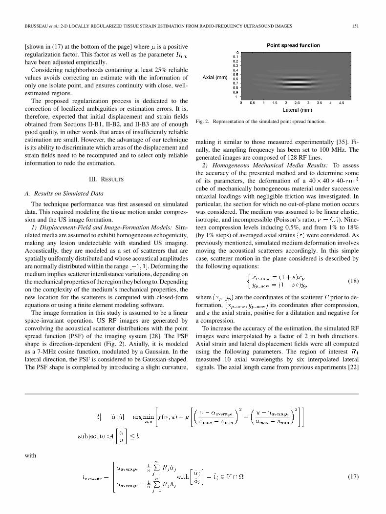
The image formation in this study is assumed to be a linearspace-invariant operation. US RF images are generated byconvolving the acoustical scatterer distributions with the pointspread function (PSF) of the imaging system [28]. The PSFshape is direction-dependent (Fig. 2). Axially, it is modeledas a 7-MHz cosine function, modulated by a Gaussian. In thelateral direction, the PSF is considered to be Gaussian-shaped.The PSF shape is completed by introducing a slight curvature,

Fig. 2. Representation of the simulated point spread function.

making it similar to those measured experimentally [35]. Fi-nally, the sampling frequency has been set to 100 MHz. Thegenerated images are composed of 128 RF lines.

2) Homogeneous Mechanical Media Results: To assessthe accuracy of the presented method and to determine someof its parameters, the deformation of a 40 40 40-cube of mechanically homogeneous material under successiveuniaxial loadings with negligible friction was investigated. Inparticular, the section for which no out-of-plane motion occurswas considered. The medium was assumed to be linear elastic,isotropic, and incompressible (Poisson’s ratio, ). Nine-teen compression levels inducing 0.5%, and from 1% to 18%(by 1% steps) of averaged axial strains were considered. Aspreviously mentioned, simulated medium deformation involvesmoving the acoustical scatterers accordingly. In this simplecase, scatterer motion in the plane considered is described bythe following equations:

(18)

where are the coordinates of the scatterer prior to de-formation, its coordinates after compression,and the axial strain, positive for a dilatation and negative fora compression.

To increase the accuracy of the estimation, the simulated RFimages were interpolated by a factor of 2 in both directions.Axial strain and lateral displacement fields were all computedusing the following parameters. The region of interestmeasured 10 axial wavelengths by six interpolated lateralsignals. The axial length came from previous experiments [22]

with

(17)


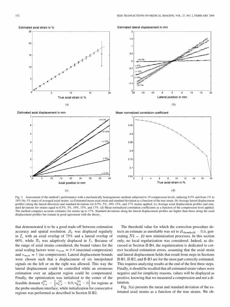
Fig. 3. Assessment of the method’s performance with a mechanically homogeneous medium subjected to 19 compression levels, inducing 0.5% and from 1% to18% (by 1% steps) of averaged axial strains. (a) Estimated mean axial strain and standard deviation as a function of the true strain. (b) Average lateral displacementprofiles (along the lateral direction) and standard deviations for 0.5%, 5%, 10% 15%, and 17% strains applied. (c) Average axial displacement profiles and stan-dard deviations for strains equal to 0.5%, 5%, 10%, 15%, and 17%. (d) Mean normalized correlation coefficients as a function of the compression level applied.The method computes accurate estimates for strains up to 17%. Standard deviations along the lateral displacement profiles are higher than those along the axialdisplacement profiles but remain in good agreement with the theory.

that demonstrated it to be a good trade-off between estimationaccuracy and spatial resolution. was displaced regularlyin with an axial overlap of 75% and a lateral overlap of60%, while was adaptively displaced in . Because ofthe range of axial strains considered, the bound values for theaxial scaling factors were (maximal compression)and (no compression). Lateral displacement boundswere chosen such that a displacement of six interpolatedsignals on the left or on the right was allowed. This way thelateral displacement could be controlled while an erroneousestimation over an adjacent region could be compensated.Finally, the optimization was initialized to the center of thefeasible domain for regions atthe probe-medium interface, while initialization for consecutiveregions was performed as described in Section II-B2.

The threshold value for which the correction procedure de-tects an estimate as unreliable was set to , gen-erating new minimization processes. In this sectiononly, no local regularization was considered. Indeed, as dis-cussed in Section II-B4, the regularization is dedicated to cor-rect localized estimation errors, assuming that the axial strainand lateral displacement fields that result from steps in SectionsII-B1, II-B2, and II-B3 are for the most part correctly estimated.This requires analyzing results at the end of the first three steps.Finally, it should be recalled that all estimated strain values werenegative and for simplicity reasons, values will be displayed aspositive, knowing that we measured a compression and not a di-latation.

Fig. 3(a) presents the mean and standard deviation of the es-timated axial strains as a function of the true strains. We ob-


serve that the method is able to accurately compute estimates forstrains up to 17%. The standard deviation increases slightly withthe deformation but remains low over the range. Axial displace-ments were computed from axial strain estimates. Their meanprofiles along the axial direction as well as standard deviationsare reported in Fig. 3(c) for a few compression levels ( ,5%, 10%, 15%, and 17%) for purposes of clarity. However, allcompression levels were investigated and it was observed a verycontinuous evolution in axial displacement mean profiles fromone level to another. Computed mean axial displacements arevery close to the theoretical values. A slight increase in standarddeviations with the compression level can be observed; howeverthey remain on the order of 1e-3 mm for . Mean profilesand standard deviations for lateral displacements are also pro-vided [Fig. 3(b)]. As expected, their estimation is noisier thanthe estimation along the axial direction, but remains in goodagreement with theoretical values. Finally, the mean correlationcoefficient as a function of the compression level is displayed[Fig. 3(d)]. Its value, close to 1 for small strains, decreases withthe applied compression to reach 0.8 for 16% strain. With in-creasing strains, signals are subjected to higher nonlinear ampli-tude and phase distortions that are not considered in our defor-mation model. Nevertheless, the technique proposed provides agood-quality estimation.

These results must, however, be cautiously interpreted, sincesimulations always remain ideal cases and the medium studiedis mechanically homogeneous and therefore uniformly absorbsthe compression. Biological tissues are unfortunately mainlyheterogeneous, especially when they are pathological. Theircompression will result in a wide range of strain variations.The load therefore needs to be carefully applied to avoid largeareas of high strains . Moreover, local strong mediumheterogeneities may increase signal distortions, reducing therange of accurate strains with the use of medical data.

However, this range will remain sufficiently wide to inves-tigate in vivo biological tissues. Previous studies concerningmedical applications have demonstrated the potential of elastog-raphy, with elastograms exhibiting a narrower range of accuratestrains [6], [9], [30].

The following results use local regularization when neces-sary. The parameters and were empirically selected usingphantom and biological tissue data. According to our observa-tions, small areas of the displacement and strain fields that visu-ally appear to suffer from an erroneous estimation were mainlycharacterized by a correlation coefficient that remained weakafter the correction procedure. These considerations have led usto set to 0.8.

Determining was achieved by varying its value in the range– and by investigating the regularization effects on the

displacement and strain fields. We visually observed that for, the regularization was too weak to smooth the areas

concerned. For , the parameter vector estimation wasexclusively dominated by the regularization process. Finally, for

, a very slow continuous area smoothing was ob-served with increasing values for the regularization factor. Con-sequently was set to 30.

3) Heterogeneous Mechanical Media Results: The abilityof the proposed technique to image heterogeneous strain fields

was investigated with two simulated linear elastic, nearly in-compressible mechanical bodies. The first case we numericallycreated was a homogeneous cube containing acylindrical inclusion that was twice as hard as the surroundingmaterial . This medium was subjected to a uni-axial load of 2 kPa. The second medium was a three-layer body,whose middle layer of Young’s modulus wassix times softer than the top and bottom layers .This body was subjected to a uniaxial load of 7 kPa. Its defor-mation covered a wider range of strains than the example usedin the first case. Both bodies measured 40 40 40 .

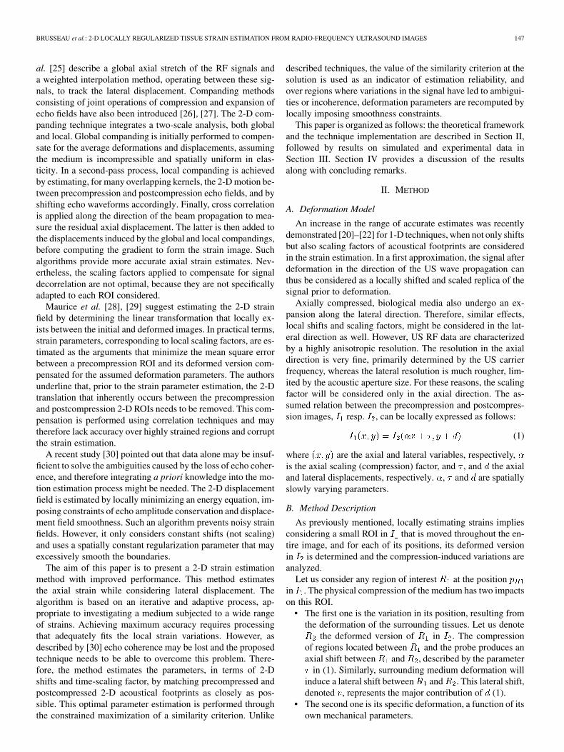
The resulting displacement and strain fields from the em-bedded inclusion medium and the three-layer medium arepresented in Figs. 4 and 5, respectively. For both, estimatedfields are close to the theoretical values. In Fig. 4(b), the axialstrain field brings out the hard inclusion with sharp boundaries,whereas it is not detectable in the conventional -scan USimage [Fig. 4(h)]. Regions located above and below the hard in-clusion exhibit higher strains because of stress concentrations,as demonstrated with the theoretical field [Fig. 4(a)]. The corre-sponding axial displacement field has been deduced [Fig. 4(d)]and is in perfect agreement with the theory [Fig. 4(c)]. In thelateral direction, the displacement field also corroborates thetheoretical values, but is noisier than the axial displacementfield, because of the poor lateral resolution of the imagingsystem. Finally, as the objective function is based on the nor-malized correlation coefficient between a 2-D initial region andits compensated deformed version, this similarity criterion hasbeen mapped. It remains strong throughout the entire image,achieving its highest values for less strained regions. Theweakest values are reached at the inclusion boundaries, wherethe assumption of a constant strain over the region of interestis not valid. However, the correlation coefficient remains highand has been estimated at 0.96 on average.

Similar observations can be made with the fields resultingfrom the three-layer medium. Estimated strain and displace-ment fields are close to FEM distributions. Correlation coef-ficients are in the range – , with more than 99% ofthem higher than 0.8, resulting in a mean value of 0.94.

B. Results on Experimental Data

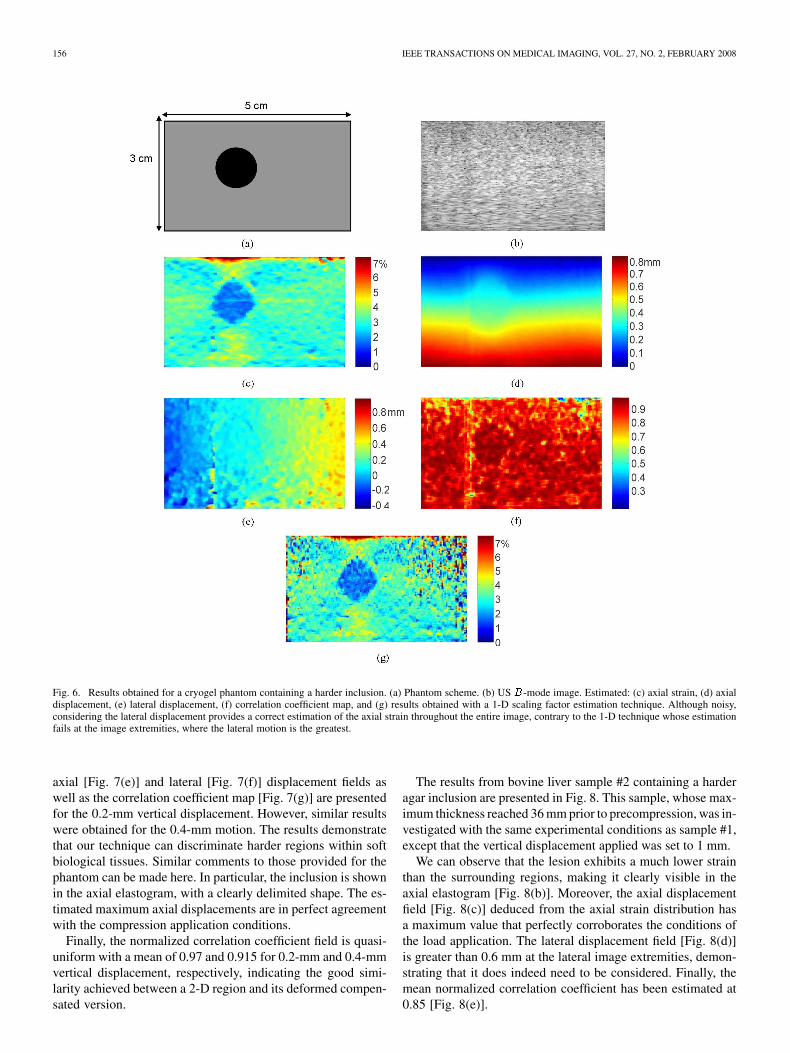
1) Strain Imaging of a Tissue-Mimicking Phantom: RF USimages were acquired from a parallelepipedic PVA cryogelphantom, measuring 3 5 4 and containing a hardercylindrical inclusion [Fig. 6(a)]. Polyvinyl alcohol (PVA)cryogel is a material whose stiffness increases by oper-ating successive freeze-thaw cycles, adapted for constructingtissue-mimicking phantoms [36]. The surrounding mediumand the inclusion were subjected to 1 and 3 freeze-thaw cycles,respectively. During the experiment, the bottom surface of thephantom lay on a support, while its top surface was compresseddownward by lowering the US probe. The other four verticalexterior phantom surfaces were free to slip. The transducer wassubjected to a 0.9-mm vertical displacement inducing a meanglobal strain of 3%. RF images were acquired with a 7-MHzcentral frequency probe and sampled with a frequency of 50MHz. Each image was composed of 128 RF A-lines. RF data


Fig. 4. Simulated inhomogeneous phantom with a harder inclusion. True: (a) axial strain, (c) axial displacement, (e) lateral displacement. Estimated: (b) axialstrain, (d) axial displacement, (f) lateral displacement. (g) Normalized correlation coefficient map, (h) B-mode image.

were interpolated by a factor of 4 in the axial direction and by afactor of 2 in the lateral direction, prior to strain computation.

Results are presented in Fig. 6. While the inclusion isnot revealed in the classical -mode US image [Fig. 6(b)],it is clearly brought out with sharp boundaries in the axialelastogram [Fig. 6(c)]. The maximal axial displacement isestimated at 0.83 mm, and the mean axial strain at 3.05%, cor-roborating the experimental conditions. Lateral displacementestimation is noisy [Fig. 6(e)] but remains in agreement with thetheoretical developments. Moreover, its significant amplitudedemonstrates that it must be taken into account for a better

estimation of the axial component. Indeed, we can observe thatalthough noisy, considering the lateral displacement provides acorrect estimation of the axial strain even at the lateral imageextremities, where the lateral motion is the greatest. This levelof quality could not be achieved with techniques that ignorethis motion, such as 1-D methods. As illustrated with the elas-togram provided in Fig. 6(g) and computed with a 1-D-scalingfactor estimation technique [22], the axial strain computationis highly corrupted by signal decorrelation toward the image’slateral borders, resulting in erroneous values. This may lead toelastogram areas where a small lesion is undetectable because


Fig. 5. Simulated three-layer phantom. True: (a) axial strain, (c) axial displacement, and (e) lateral displacement. Estimated: (b) axial strain, (d) axial displacement,and (f) lateral displacement. (g) Normalized correlation coefficient map. (h) B-mode image.

of the noise level. With such 1-D schemes, the loss of correla-tion induced by lateral motion cannot be compensated for byadditional processing.

Finally, the distribution of the normalized correlation coeffi-cient between an initial 2-D region and its deformed version,compensated for the lateral shift and axial scaling factor, isquasi-uniform and estimated on average at 0.89 [Fig. 6(f)].

2) Strain Imaging of In Vitro Bovine Livers: Our method wasfinally tested on experimental data from two cut specimens ofbovine liver [Fig. 7(a)]. The first biological sample presentedvariable thicknesses with a maximum of 28 mm. An embeddedharder inclusion in agar gel measuring approximately 7.5 mm

in diameter was created inside the soft tissue [Fig. 7(b)]. Thesame experimental protocol as described in the previous sectionwas applied, with the two following differences. The verticaldisplacement of the probe to perform the compression was de-creased to 0.2 and 0.4 mm because of the weak thickness of thetissue, emphasized by the significant precompression that needsto be applied to ensure sufficient contact between the transducerand the curved top surface of the specimen. Moreover, the sam-pling frequency was set at 200 MHz. Data were interpolated bya factor of 2 in the lateral direction.

Fig. 7 illustrates the axial strain fields for 0.2 mm [Fig. 7(d)]and 0.4 mm [Fig. 7(h)] of vertical displacements. The estimated


Fig. 6. Results obtained for a cryogel phantom containing a harder inclusion. (a) Phantom scheme. (b) US B-mode image. Estimated: (c) axial strain, (d) axialdisplacement, (e) lateral displacement, (f) correlation coefficient map, and (g) results obtained with a 1-D scaling factor estimation technique. Although noisy,considering the lateral displacement provides a correct estimation of the axial strain throughout the entire image, contrary to the 1-D technique whose estimationfails at the image extremities, where the lateral motion is the greatest.

axial [Fig. 7(e)] and lateral [Fig. 7(f)] displacement fields aswell as the correlation coefficient map [Fig. 7(g)] are presentedfor the 0.2-mm vertical displacement. However, similar resultswere obtained for the 0.4-mm motion. The results demonstratethat our technique can discriminate harder regions within softbiological tissues. Similar comments to those provided for thephantom can be made here. In particular, the inclusion is shownin the axial elastogram, with a clearly delimited shape. The es-timated maximum axial displacements are in perfect agreementwith the compression application conditions.

Finally, the normalized correlation coefficient field is quasi-uniform with a mean of 0.97 and 0.915 for 0.2-mm and 0.4-mmvertical displacement, respectively, indicating the good simi-larity achieved between a 2-D region and its deformed compen-sated version.

The results from bovine liver sample #2 containing a harderagar inclusion are presented in Fig. 8. This sample, whose max-imum thickness reached 36 mm prior to precompression, was in-vestigated with the same experimental conditions as sample #1,except that the vertical displacement applied was set to 1 mm.

We can observe that the lesion exhibits a much lower strainthan the surrounding regions, making it clearly visible in theaxial elastogram [Fig. 8(b)]. Moreover, the axial displacementfield [Fig. 8(c)] deduced from the axial strain distribution hasa maximum value that perfectly corroborates the conditions ofthe load application. The lateral displacement field [Fig. 8(d)]is greater than 0.6 mm at the lateral image extremities, demon-strating that it does indeed need to be considered. Finally, themean normalized correlation coefficient has been estimated at0.85 [Fig. 8(e)].


Fig. 7. Results from bovine liver sample #1 within which is embedded a harder inclusion in agar. (a) Global view of the biological sample. (b) Photograph of theslice of interest. (c) USB-mode image. Estimated: (d) axial strain, (e) axial displacement, (f) lateral displacement, and (g) normalized correlation coefficient, for avertical displacement of 0.2 mm, and (h) axial strain for a 0.4-mm probe motion applied. Whereas the agar inclusion is nearly undetectable in the B-mode image,it is clearly visible in the deformation fields. Moreover, the difference in range of axial strain fields (d) and (h) as well as the axial displacement distribution are inperfect agreement with the experimental conditions of the load application.

IV. CONCLUSION

In this paper, a 2-D strain estimation algorithm was intro-duced, computing the axial strain while considering lateral mo-tion. Contrary to most 2-D techniques that model the compres-sion-induced local displacement as a 2-D shift, we also considera scaling factor in the axial dimension. This leads to a methodthat is much more robust in terms of decorrelation noise and re-sults in a larger range of accurate measurements.

To achieve maximum accuracy, the technique computes de-formation parameters as those leading to the best possible matchbetween the precompression and postcompression 2-D RF re-gions, when the latter are highly correlated. This is done throughthe constrained maximization of an objective function, definedas the normalized correlation coefficient between the initial 2-DRF acoustical region and the deformed region, compensated forthe deformation parameters. When the correlation is lost, the

estimation integrates an additional local smoothness constraint,imposing the continuity of resulting displacement and strainfields.

Two error sources for the model (1) should nevertheless bementioned. The processed RF images inevitably contain anadditive noise that can be modeled as a signal-independent,zero-mean, spatially uncorrelated process like electronic noise[18]. However, the similarity criterion used is known to berobust to such noise [37]. Moreover, with increasing strains,signals will be subjected to higher nonlinear amplitude andphase distortions that are not considered in our deformationmodel. This represents the major cause of decorrelation atlarger strains.

The results on phantom and in vitro biological data demon-strate the ability of our technique to image deformation, pro-viding information complementary to standard US images.


Fig. 8. Results from bovine liver sample #2. (a) USB-mode image. Estimated: (b) axial strain, (c) axial displacement, (d) lateral displacement, and (e) normalizedcorrelation coefficient for a 1-mm vertical displacement of the probe. Agar inclusion exhibits a much lower strain than the surrounding medium.

Compared to 1-D techniques, the algorithm described is char-acterized by a significant increase of computational costs. Withthe current implementation, the run time to compute one axialstrain image and the corresponding lateral field is a few min-utes on a PC (Pentium M 1.7-GHz Processor, 1GB. RAM). De-veloping a real-time method is beyond the scope of this paper.However, it has to be mentioned that the algorithm can be mod-ified to support parallel computing. Investigating such imple-mentation will be part of our future work.

In the present implementation, bounds of the feasible regionand thresholds are constants. It should be possible to adapt themaccording to the estimated compression level. This could accel-erate theconvergenceof thealgorithm.Therefore theseparametervalues may evolve with future analysis. Finally, the present algo-rithm, based on the sequential quadratic programming method-ology, allows the immediate addition of new constraints, whetherlinear or nonlinear. It can also be easily formalized in 3-D.

APPENDIX

A. The Sequential Quadratic Programming (sequential QP)Algorithm is a generalization of Newton’s method, in thatit finds a step away from the current point by minimizing aquadratic model of the problem.

Given initializations, , , , the

technique consists in iteratively:1) Forming and solving the (QP) subproblem to obtain the

descent direction (see Appendix B).2) Determining a step length to obtain a sufficient decrease

in the objective function.3) Set and updates the Lagrange multi-

pliers.4) STOP if convergence ( satisfaction of the Kuhn–Tucker

conditions).5) Else compute (BFGS update), set and go

to 1).B. Form and Solve the (QP) Subproblem: The descent di-

rection is computed as the solution of the associated QP sub-problem. In our case, it corresponds to finding the constrainedminimum of the quadratic approximation of the objective func-tion since all constraints are linear

subject to:

where .


Fig. 9. QP solution computation.

This problem is solved by using an active set strategy. Ac-tive set methods are procedures that aim at identifying the con-straints that will become active at the solution. Since it is notpossible to know a priori which constraints will be active at thesolution, these techniques are based on developing a predictionof the correct active set. And because the prediction could bewrong, the technique must also include procedures to modify it.

In the article, we denoted the submatrix of containingthe coefficients of the constraints active at the solution andthe matrix whose columns form a basis for the set of vectorsorthogonal to the rows of . thus defined the subspace offeasible search directions.

Similarly, we will denote the prediction of the active set atthe th iteration and the corresponding subspace of feasibledirections.

The technique works as shown in Fig. 9. In most cases, thisprocess is completed in 1 or 2 iterations.

REFERENCES

[1] J. Ophir, I. Céspedes, H. Ponnekanti, Y. Yazdi, and X. Li, “Elastog-raphy: A quantitative method for imaging the elasticity of biologicaltissues,” Ultrason. Imag., vol. 13, pp. 111–134, 1991.

[2] W. A. D. Anderson and J. M. Kissane, Pathology, 9th ed. St. Louis,MO: Mosby, 1953.

[3] T. A. Krouskop, T. M. Wheeler, F. Kallel, B. S. Garra, and T. Hall,“Elastic moduli of breast and prostate tissues under compression,” Ul-trason. Imag., vol. 20, pp. 260–274, 1998.

[4] B. S. Garra, E. I. Céspedes, J. Ophir, S. R. Spratt, R. A. Zuurbier, C. M.Magnant, and M. F. Pennanen, “Elastography of breast lesions: Initialclinical results,” Radiology, vol. 202, pp. 79–86, 1997.

[5] L. Sandrin, B. Fourquet, J. M. Hasquenoph, S. Yon, C. Fournier, F.Mal, C. Christidis, M. Ziol, B. Poulet, F. Kazemi, M. Beaugrand, andR. Palau, “Transient elastography: A new noninvasive method for as-sessment of hepatic fibrosis,” Ultrasound Med. Biol., vol. 29, no. 12,pp. 1705–1713, 2003.

[6] C. L. De Korte, S. G. Carlier, F. Mastik, M. M. Doyley, A. F. W. VanDer Steen, P. Serruys, and N. Bom, “Morphological and mechanicalinformation of coronary arteries obtained with intravascular elastog-raphy—Feasibility study in vivo,” Eur. Heart J., no. 23, pp. 405–413,2002.

[7] C. L. D. Korte, G. Pasterkamp, A. F. W. van der Steen, H. A. Woutman,and N. Bom, “Characterization of plaque components with intravas-cular ultrasound elastography in human femoral and coronary arteriesin vitro,” Circulation, vol. 102, pp. 617–23, 2000.

[8] E. Brusseau, J. Fromageau, G. Finet, P. Delachartre, and D. Vray,“Axial strain imaging of intravascular data: Results on polyvinylalcohol cryogel phantoms and a carotid artery,” Ultrasound Med. Biol.,vol. 27, no. 12, pp. 1631–1642, 2001.

[9] R. Souchon, O. Rouviere, A. Gelet, V. Detti, S. Srinivasan, J. Ophir,and J. Y. Chapelon, “Visualisation of HIFU lesions using elastographyof the human prostate in vivo: Preliminary results,” Ultrasound Med.Biol., vol. 29, no. 7, pp. 1007–15, 2003.

[10] Y. Mofid, F. Ossant, F. Kathyr, M. Limberis, and F. Patat, “In vivohuman skin elastography: Preliminary study,” in Proc. World CongressUltrasonics, 2003, pp. 205–208.

[11] J. L. Genisson, T. Baldeweck, M. Tanter, S. Catheline, M. Fink,L. Sandrin, C. Cornillon, and B. Querleux, “Assessment of elasticparameters of human skin using dynamic elastography,” IEEE Trans.Ultrason., Ferroelect., Freq. Contr., vol. 51, no. 8, pp. 980–989,Aug. 2004.

[12] S. Emelianov, M. A. Lubinski, W. F. Weitze, R. C. Wiggins, A. R.Skovoroda, and M. O’Donnell, “Elasticity imaging for early detectionof renal pathology,” Ultrasound Med. Biol., vol. 21, no. 7, pp. 871–883,1995.

[13] C. L. de Korte, A. F. W. van der Steen, B. H. J. Dijkman,and CT. Lancée, “Performance of time delay estimation methodsfor small time shifts in ultrasonic signals,” Ultrasonics, vol. 35,pp. 263–274, 1997.

[14] X. Lai and H. Torp, “Interpolation methods for time-delay estimationusing cross-correlation method for blood velocity measurement,” IEEETrans. Ultrason., Ferroelectr., Freq. Contr., vol. 46, no. 2, pp. 277–290,Mar. 1999.

[15] X. L. Xu, A. H. Tewfik, and J. F. Greenleaf, “Time delay estimationusing wavelet transform for pulsed-wave ultrasound,” Ann. Biomed.Eng., vol. 23, no. 5, pp. 612–621, 1995.


[16] J. Luo, J. Bai, P. He, and K. Ying, “Axial strain calculation using alow-pass digital differentiator in ultrasound elastography,” IEEE Trans.Ultrason., Ferroelect., Freq. Contr., vol. 51, no. 9, pp. 1119–1127, Sep.2004.

[17] A. Pesavento, C. Perrey, M. Krueger, and H. Ermert, “A time-efficientand accurate strain estimation concept for ultrasonic elastography usingiterative phase zero estimation,” IEEE Trans. Ultrason., Ferroelect.,Freq. Contr., vol. 46, no. 5, pp. 1057–1067, Sep. 1999.

[18] M. Bilgen and M. F. Insana, “Deformation models and correlation anal-ysis in elastography,” J. Acoust. Soc. Am., vol. 99, no. 5, pp. 3212–3224,1996.

[19] M. Bilgen and M. F. Insana, “Error analysis in acoustic elastography.I. Displacement estimation,” J. Acoust. Soc. Am., vol. 101, no. 2, pp.1139–1146, 1997.

[20] S. K. Alam, J. Ophir, and E. E. Konofagou, “An adaptive strain es-timator for elastography,” IEEE Trans. Ultrason., Ferroelect., Freq.Contr., vol. 45, no. 2, pp. 461–472, Mar. 1998.

[21] M. Bilgen, “Wavelet-based strain estimator for elastography,” IEEETrans. Ultrason., Ferroelect., Freq. Contr., vol. 46, pp. 1407–1415,1999.

[22] E. Brusseau, C. Perrey, P. Delachartre, M. Vogt, D. Vray, and H. Er-mert, “Axial strain imaging using a local estimation of the scalingfactor from RF ultrasound signals,” Ultrason. Imag., vol. 22, no. 2, pp.95–107, 2000.

[23] M. O’Donnell, A. R. Skovoroda, B. M. Shapo, and S. Y. Emelianov,“Internal displacement and strain imaging using ultrasonic speckletracking,” IEEE Trans. Ultrason., Ferroelect., Freq. Contr., vol. 41,pp. 314–324, 1994.

[24] X. Chen, M. J. Zohdy, S. Y. Emelianov, and M. O’Donnell, “Lateralspeckle tracking using synthetic lateral phase,” IEEE Trans. Ultrason.,Ferroelect., Freq. Contr., vol. 51, no. 5, pp. 540–550, May 2004.

[25] E. E. Konofagou and J. Ophir, “A new elastographic method for esti-mation and imaging of lateral displacements, lateral strains, correctedaxial strains and Poisson’s ratio in tissues,” Ultrasound Med. Biol., vol.24, no. 8, pp. 1183–1199, 1998.

[26] P. Chaturvedi, M. F. Insana, and T. J. Hall, “2-D companding for noisereduction in strain imaging,” IEEE Trans. Ultrason., Ferroelec., Freq.Contr., vol. 45, no. 1, pp. 179–191, Jan. 1998.

[27] P. Chaturvedi, M. F. Insana, and T. J. Hall, “Testing the limitationsof 2-D companding for strain imaging using phantoms,” IEEE Trans.Ultrason., Ferroelec., Freq. Contr., vol. 45, no. 4, pp. 1022–1031, Jul.1998.

[28] R. L. Maurice, J. Ohayon, Y. Frétigny, M. Bertrand, G. Soulez, andG. Cloutier, “Non-invasive vascular elastography: Theoretical frame-work,” IEEE Trans. Med. Imag., vol. 23, no. 2, pp. 164–180, Feb. 2004.

[29] R. L. Maurice and M. Bertrand, “Lagrangian speckle model and tissue-motion estimation—Theory,” IEEE Trans. Med. Imag., vol. 18, no. 7,pp. 593–603, Jul. 1999.

[30] C. Pellot-Barakat, F. Frouin, M. F. Insana, and A. Herment, “Ultra-sound elastography based on multiscale estimations of regularized dis-placement fields,” IEEE Trans. Med. Imag., vol. 23, no. 2, pp. 153–63,Feb. 2004.

[31] P. T. Boggs and J. W. Tolle, “Sequential quadratic programming,” ActaNumerica, vol. 4, pp. 1–51, 1996.

[32] P. E. Gill, W. Murray, and M. H. Wright, Practical Optimization.New York: Academic, 1981.

[33] F. Heitz, P. Perez, and P. Bouthemy, “Multiscale minimization ofglobal energy functions in some visual recovery problems,” CVGIP:Image Understand., vol. 59, no. 1, pp. 125–134, 1994.

[34] Y. C. Fung, Biomechanics—Mechanical Properties of Living Tissues,2nd ed. New York: Springer-Verlag, 1993.

[35] H. Du, J. Liu, C. Pellot Barakat, and M. F. Insana, “Optimizing multi-compression approaches to elasticity imaging,” IEEE Trans. Ultrason.,Ferroelect., Freq. Contr., vol. 53, no. 1, pp. 90–99, Jan. 2006.

[36] K. C. Chu and B. K. Rutt, “Polyvinyl alcohol cryogel: An idealphantom material for MR studies of arterial flow and elasticity,” Magn.Reson. Med., vol. 37, no. 2, pp. 314–319, 1997.

[37] F. Viola and W. F. Walker, “Comparison of time-delay estimators inmedical ultrasound,” in Proc. IEEE Ultrason. Symp., Oct. 2001, vol. 2,pp. 1485–1488.

IEEE TRANSACTIONS ON MEDICAL IMAGING, VOL. 27, NO. 2 ...

Documents

Transcript of IEEE TRANSACTIONS ON MEDICAL IMAGING, VOL. 27, NO. 2 ...