IEEE TRANSACTIONS ON MEDICAL IMAGING, VOL. 23, NO…bouman/publications/orig-pdf/tmi2.pdf ·...

IEEE TRANSACTIONS ON MEDICAL IMAGING, VOL. 23, NO. 1, JANUARY 2004 85

Clustered Components Analysis for Functional MRISea Chen, Member, IEEE, Charles A. Bouman*, Fellow, IEEE, and Mark J. Lowe

Abstract—A common method of increasing hemodynamicresponse (SNR) in functional magnetic resonance imaging (fMRI)is to average signal timecourses across voxels. This technique ispotentially problematic because the hemodynamic response mayvary across the brain. Such averaging may destroy significantfeatures in the temporal evolution of the fMRI response that stemfrom either differences in vascular coupling to neural tissue oractual differences in the neural response between two averagedvoxels. Two novel techniques are presented in this paper inorder to aid in an improved SNR estimate of the hemodynamicresponse while preserving statistically significant voxel-wisedifferences. The first technique is signal subspace estimation forperiodic stimulus paradigms that involves a simple thresholdingmethod. This increases SNR via dimensionality reduction. Thesecond technique that we call clustered components analysis isa novel amplitude-independent clustering method based uponan explicit statistical data model. It includes an unsupervisedmethod for estimating the number of clusters. Our methodsare applied to simulated data for verification and comparisonto other techniques. A human experiment was also designed tostimulate different functional cortices. Our methods separatedhemodynamic response signals into clusters that tended to beclassified according to tissue characteristics.

Index Terms—BOLD signal estimation, brain activation, clus-tering methods, EM algorithm, functional MRI, functional neu-roimaging, hemodynamic response, independent components anal-ysis, vascular coupling.

I. INTRODUCTION

FUNCTIONAL magnetic resonance imaging (fMRI) hasemerged as a useful tool in the study of brain function.

This imaging modality utilizes the fact that the MRI signal issensitive to many of the hemodynamic parameters that changeduring neuronal activation (e.g., blood flow, blood volume, andoxygenation). The changes in these parameters cause smallintensity differences between properly weighted MR imagesacquired before and during neuronal activation. Although thecontrast can be produced by a number of different mechanisms,blood oxygenation level dependent (BOLD) contrast is the

Manuscript received April 9, 2003; revised July 10, 2003. This work wassupported in part by the National Science Foundation (NSF) IGERT PTDDunder Training Grant DGE-99-72770. The Associate Editor responsible forcoordinating the review of this paper and recommending its publication wasZ. P. Liang. Asterisk indicates corresponding author.

S. Chen is with the Division of Imaging Sciences, Department of Radiology,Indiana University, School of Medicine, Indianapolis, IN, and the Departmentof Biomedical Engineering, Purdue University, West Lafayette, IN 47907 USA(e-mail: [email protected]).

*C. A. Bouman is with the School of Electrical and Computer En-gineering, Purdue University, West Lafayette, IN 47907 USA (e-mail:[email protected]).

M. J. Lowe is with the Division of Imaging Sciences, Department of Radi-ology, Indiana University, School of Medicine, Indianapolis, IN, and the Depart-ment of Biomedical Engineering, Purdue University, West Lafayette, IN 47907USA (e-mail: [email protected]).

Digital Object Identifier 10.1109/TMI.2003.819922

method most commonly employed. BOLD contrast is depen-dent on an decrease in local deoxy-hemoglobin concentrationin an area of neuronal activity [1], [2]. This local decreasein paramagnetic material increases the apparent transverserelaxation constant , resulting in an increase of MR signalintensity in the area affected. Other methods of functional MRimaging contrast include measurement of cerebral blood flowand volume effects [3]. Although fMRI is widely used, themechanism of the coupling between brain hemodynamics andneuronal activation is poorly understood.

Although much of the work in fMRI data analysis has re-volved around the creation of statistical maps and the detec-tion of activation at different voxel locations [4]–[6], there alsohas been much interest in understanding the BOLD temporal re-sponse. Several groups have proposed models relating the var-ious hemodynamic parameters (blood flow, blood volume, he-moglobin concentration, etc.) to the BOLD signal [7], [8]. Thesemodels all predict a BOLD temporal response to changing neu-ronal activity. Verification of the accuracy of these models re-quires that the predictions be compared to data. However, thelow signal-to-noise ratio (SNR) of fMRI measurements typi-cally requires averaging of many voxels in order to achieve astatistically significant result. Thus, the resulting measurementcould possibly be a mixture of many different responses. Thispresents a possible confound in attempts to develop and validatedetailed models of the BOLD response.

Some researchers have attempted to address the issue byusing parametric methods [9], [10]. The parametric methodsusually assume specific signal shapes (Poisson, Gaussian,Gamma, etc.) and attempt to extract the associated parametersfor which the data best fit. Others have taken a linear systemsapproach in which the response is modeled as an impulseresponse convolved with the stimulus reference function [11],[12]. Exploratory data analysis methods such as principal com-ponents analysis (PCA) [13], [14] and independent componentsanalysis (ICA) [15], [16] are also commonly used by manygroups. Recently, clustering methods [17]–[20] have becomepopular as well.

In this paper, we address the issue of signal averaging bypresenting a novel nonparametric clustering method basedupon a statistical data model. Our technique is designed torobustly estimate the fMRI signal waveforms rather than detecttheir presence. Specifically, we first select voxels that containthe fMRI signal using a previously published technique [21].Then our procedure identifies groups of voxels in fMRI datawith the same temporal shape independent of signal amplitude.Variations in amplitudes may be due to differences in theconcentration of hemodynamic events from partial volumeeffects or coil geometries. The amplitude variation is explicitlyaccounted for in our data model. Each distinct response cor-responds to a unique direction in a multidimensional featurespace (see Fig. 1).

0278-0062/04$20.00 © 2004 IEEE

86 IEEE TRANSACTIONS ON MEDICAL IMAGING, VOL. 23, NO. 1, JANUARY 2004

Fig. 1. Visualization of cylindrical clusters extracted by CCA: Because CCAfinds cluster directions independent of amplitude, the shape of the vector cloudswill be cylindrical instead of the more common spherical clouds around classmeans extracted by other clustering methods.

Our analysis framework is based upon two distinct steps. Inthe first step, the dimensionality of the voxel timecourses is re-duced and feature vectors are obtained. The noise in the featurevectors is then whitened. The second step consists of our novelclustering technique that we call clustered components analysis(CCA).1

The dimensionality reduction used in this paper is similar tothe method described by Bullmore, et al. [22]. Their methoddecomposes the temporal response at each voxel into harmoniccomponents corresponding to a sine and cosine series expansionat the appropriate period. We have developed a method to furtherdecrease dimensionality by estimating an -dimensional signalsubspace [23]. Although signal subspace estimation (SSE) is notnew [24], [25], our method uses a simple thresholding techniqueand is quite effective. It is implemented by estimating the signalcovariance as the positive definite part of the difference betweenthe total signal-plus-noise covariance and the noise covariance.At this point in our analysis technique, each voxel’s response isrepresented by an dimensional feature vector.

In the second step of our analysis framework, we present anew method for analyzing the multivariate fMRI feature vectorsthat we call CCA. This method depends on a explicit data modelof the feature vectors and is implemented through maximum-likelihood (ML) estimation via the expectation-maximization(EM) algorithm [26], [27]. An agglomerative cluster mergingtechnique based on a minimum description length (MDL) crite-rion [28] is used to estimate the true number of clusters [29].

Because the truth is not known in a real experiment, syntheticdata was generated to test the performance of our method.Other common methods of multivariate data-driven analysistechniques (PCA, ICA, and fuzzy clustering) were applied tothe same data set and the results were compared. Finally, ahuman experiment was performed that stimulated the motor,visual, and auditory cortices. Our methodology was applied tothis data. The goal of the human experiment was to produce aset of activation data spanning a broad range of cerebral cortexand a diverse set of neuronal systems. This data set will allowour clustering method to determine the distribution of distincttemporal responses according either to neuronal system ortissue characteristics.

1CCA software is available from www.ece.purdue.edu/~bouman.

II. THEORY

A. Dimensionality Reduction

The first step of our analysis framework is the reduction ofdimensionality via decomposition into harmonic componentsusing least squares fitting. This step is similar to that describedin [22]. The next step is a novel method of determining the signalsubspace by estimating signal and noise covariances and per-forming an eigendecomposition. The final step is a prewhiteningof the noise before application of the CCA.

1) Decomposition Into Harmonic Components: In a stan-dard block paradigm, control and active states are cycled in aperiodic manner during the fMRI experiment. Therefore, the re-sponse signal should also be periodic. By assuming periodicity,harmonic components can be used as a basis for decompositionto reduce dimensionality. However, application of the period-icity constraint is not necessary for the technique described inthe next section.

The data set of an fMRI experiment, , can be defined as anmatrix, where is the number of voxels and is the

number of time points. We first remove the baseline and lineardrift components of fMRI data as a preprocessing step [21]. Thecolumns of are then zero mean, zero drift versions of the voxeltimecourses.

The harmonic components, , are a sampling of sinesand cosines at the fundamental frequency of the experimentalparadigm, (in radians/s), and its higher harmonics. Thenumber of harmonic components, , is limited by the re-quirement that there be no temporal aliasing. In other words,

where is the temporal sampling period

for(1)

We then form a design matrix

(2)

where is a column vector formed by sampling the th har-monic component at the times corresponding to the voxel sam-ples. Using this notation, the data can then be expressed as ageneral linear model [6] where

(3)

is an harmonic image matrix containing the linearcoefficients, and is the dimensional noise matrix.

Assuming all information in the signal is contained within therange , an estimate can be computed using a least squaresfit, resulting in

(4)

where the residual error is given by

(5)

(6)

(7)

The data set can be expressed in terms of the estimate of thecoefficient matrix and the residuals matrix

(8)

CHEN et al.: CCA FOR FUNCTIONAL MRI 87

We denote the estimation error as , where

(9)

(10)

2) Signal Subspace Estimation: Our next objective is toidentify the subspace of the harmonic components that spansthe space of all response signals. This signal subspace methodimproves the SNR by reducing the dimensionality of the data.

The covariance matrices for the signal, signal-plus-noise, andthe noise are defined by the following relations:

Since we cannot observe directly, we must first estimateand , and then use these matrices to estimate . With thisin mind, we use the following two estimates for and

(11)

(12)

where is computed using (6). The expression for is derivedin Appendix I using the assumption that the noise is white andis shown to be an unbiased estimate for . Note that the de-nominator of the expression reflects the additional reduction indegrees of freedom when the two drift components are removed.Since and are both unbiased estimates of the true co-variances, we may form an unbiased estimate of the signal co-variance as

(13)

The corresponding eigendecomposition is then

(14)

Generally, the matrix will have both positive and negativeeigenvalues because it is formed by the subtraction of (13).However, negative eigenvalue in are nonphysical since weknow that is a covariance matrix with strictly positive eigen-values. Therefore, we know that the subspace corresponding tothe negative eigenvalues is dominated by noise. We may exploitthis fact by removing the energy in this noise subspace. To dothis, we form a new diagonal matrix , which con-tains only the positive diagonal elements in , and we forma new modified eigenvector matrix consisting of thecolumns of corresponding to the positive eigenvalues in .The reduced dimension signal component, or eigenimage, canthen be written as

(15)

The eigenimage contains the linear coefficients for theeigensequences .

The CCA presented in the following section assumes that thenoise is white. Therefore, we apply a whitening filter to form

(16)

as described in Appendix II. The column vectors of corre-spond to dimensional feature vectors that describe the time-course of each voxel. The timecourse realizations of the indi-vidual voxels may be reconstructed via the following relation:

(17)

B. Clustered Component Analysis

The method of CCA is developed in this section. The goal ofthe method is to cluster voxels into groups that represent similarshapes and to estimate the representative timecourses. Specifi-cally, we apply the analysis to the feature vectors found in(16). The analysis not only allows for the estimation of clustertimecourses, but also estimates the total number of clusters au-tomatically. The algorithm consists of two steps. The first stepis the estimation of the timecourses using the EM algorithm.Estimation of the number of clusters occurs in the second stepusing the MDL criterion. The diagram of Fig. 2 illustrates thebasic flow of the CCA algorithm, and Fig. 3 give a detailed pseu-docode specification of the CCA algorithm.

1) Data Model: Let be the th column of the matrixfound in (16). is a vector of parameters specifying the time-course or the dimensional feature vector for voxel . Fur-thermore, let be the zero mean, zero driftcomponent directions (representing clusters) in the featurespace, each with unit norm .The basic data model can be written as

(18)

where is the unknown amplitude for voxelis the class of the voxel, and is zero mean, Gaussian noise.

Because the data have been whitened, we assume that. The probability density function of the voxel

can be stated as

(19)

with log-likelihood function being

(20)

In order to resolve the dependence on the unknown ampli-tude, the ML estimate of the amplitude is found

(21)

The amplitude estimate in (21) is then substituted into the log-likelihood of (20)

(22)


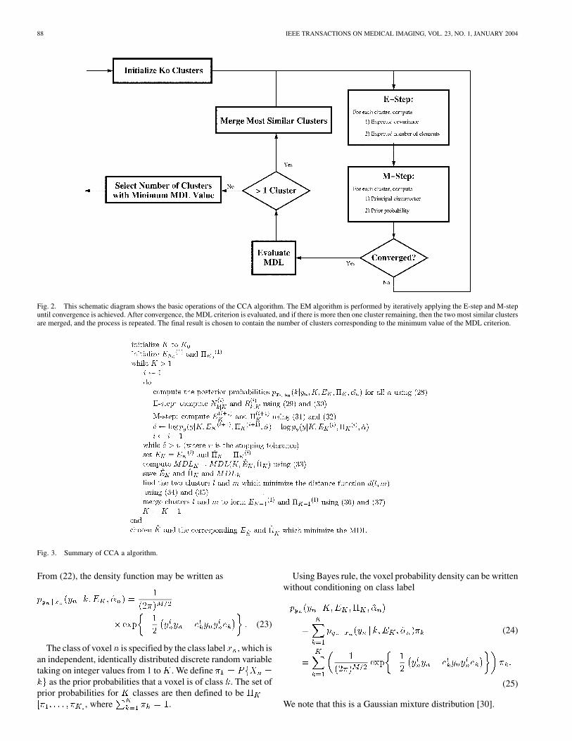
Fig. 2. This schematic diagram shows the basic operations of the CCA algorithm. The EM algorithm is performed by iteratively applying the E-step and M-stepuntil convergence is achieved. After convergence, the MDL criterion is evaluated, and if there is more then one cluster remaining, then the two most similar clustersare merged, and the process is repeated. The final result is chosen to contain the number of clusters corresponding to the minimum value of the MDL criterion.

Fig. 3. Summary of CCA a algorithm.

From (22), the density function may be written as

(23)

The class of voxel is specified by the class label , which isan independent, identically distributed discrete random variabletaking on integer values from 1 to . We define

as the prior probabilities that a voxel is of class . The set ofprior probabilities for classes are then defined to be

, where .

Using Bayes rule, the voxel probability density can be writtenwithout conditioning on class label

(24)

(25)

We note that this is a Gaussian mixture distribution [30].


The log-likelihood is then calculated for the whole set ofvoxels

(26)

2) Parameter Estimation Using the Expectation-Maximiza-tion Algorithm: The aim of this section is to estimate the pa-rameters and in the data model. This is done by findingthe ML estimates for the log-likelihood given in (26) for a givencluster number

(27)

The ML estimates and in (27) are found by using theEM algorithm [26], [30].

In order to compute the expectation step of the EM algorithm,we must first compute the posterior probability that each voxellabel is of class

(28)

In the expectation step of the EM algorithm, the estimatednumber of voxels per class and the estimated unnormal-

ized covariance matrix of the class given the current es-

timation of the parameters and must be computed.See Appendix III-A for more details. Because the EM algo-rithm is iterative, the superscripts denote iteration number.The subscript denotes the parameter corresponding to the

th cluster out of a total of clusters

(29)

(30)

In the maximization step of the EM algorithm, the parametersare reestimated from the values found in the expectation step[see (29) and (30)], yielding and . Letbe the principal eigenvector of

(31)

(32)

for (see Appendix III-B for more details).Equations (31) and (32) are alternately iterated with (29) and

(30) [using (28)]. The iterations are stopped when the differencein the log-likelihood [see (26)] for subsequent iterations is lessthan an arbitrary stopping criterion, . We then denote the finalestimates of the parameters for a given number of clusters as

and .

3) Model Order Identification: Our objective is not only toestimate the component vectors and the prior probabili-ties from observations, but also to estimate the number ofclasses . We use the MDL criterion developed by Rissanen[28], which incorporates a penalty term . Theterm represents the number of scalar values required torepresent the data, and the term represents the number ofscalar parameters encoded by and

(33)

The MDL criterion is then minimized with respect to . Thisis done by starting with large, and then sequentially mergingclusters until . More specifically, for each value of ,the values of , and are calculatedusing the EM algorithm from Section II-B2. Next, the two mostsimilar clusters are merged, is decremented to , and theprocess is repeated until . Finally, we select the value of

(and corresponding parameters and ) that resulted inthe smallest value of the MDL criterion.

This merging approach requires that we define a method forselecting similar clusters. For this purpose, we define the fol-lowing distance function between the clusters and :

(34)

where denotes the principal eigenvalue of . InAppendix IV, we show that this distance function is an upperbound on the change in the MDL value [see (66)]. Therefore,by choosing the two clusters and that minimize the clusterdistance

(35)

we minimize an upper bound on the resulting MDL criterion.The parameters of the new cluster formed by merging andare given by

(36)

(37)

The remaining cluster parameters stay constant, and the mergedparameters then become the initial parameters for the iterationsof the EM algorithm used to find estimates for clusters.

To start the algorithm, a large number of clusters ischosen. For each class

(38)

the parameters and must be initialized. The parame-

ters are initialized uniformly as

(39)

The first component directions, are initialized to theprincipal eigenvectors of the estimated data covariance matrixgiven by

(40)


Fig. 4. Experimental paradigm timing.

The remaining components are initialized by randomlysampling the normalized data vectors .

III. METHODS

A. Experimental Paradigm

An experimental paradigm was designed to activate the au-ditory, visual, and motor cortices. The paradigm was arrangedso all activation occurred in sync at a cycle length of 64 s (32s control, 32 s active). The timing of the paradigm was as fol-lows: 16 s lead in (control), four cycles of the paradigm (4 64s), 32 s control, and 16 s lead out (control). See Fig. 4 for adiagram of paradigm timing. The visual cortex was activatedusing a flashing 8-Hz checkerboard pattern (6 8 squares) witha blank screen control state viewed through fiber-optic goggles(Avotec, Inc., Stuart, FL). The flashing checkerboard has beenshown to provide robust activation throughout the visual system[31]. The auditory cortex was activated using backward speechthrough pneumatic headphones (Avotec). The backward speechhas been shown to provide robust activation in the primary audi-tory cortex [32]. Auditory control was silence through the head-phones (note that the ambient scanner noise is heard by thesubject throughout the scan). The visual and auditory stimuliwere constructed using commercial software (Adobe AfterEf-fects, Adobe Systems, Inc., San Jose, CA). The motor cortexwas activated through a complex finger-tapping task. Left andright fingers were placed opposed in a mirror-like fashion in therest position and tapped together in a self paced way in the fol-lowing pattern for activation: thumb, middle, little, index, ring,repeat. This complex finger-tapping task has been shown to pro-vide robust motor cortex activation [33]. Tapping was cued bythe onset of visual and auditory stimuli. Rest was the controlstate for the motor paradigm.

B. Human Data Acquisition

Whole-brain images of a healthy subject were obtained usinga 1.5 T GE Echospeed MRI Scanner (GE Medical Systems,Waukeshau, WI). Axial 2D spin echo -weighted anatomic im-ages were acquired for reference with the following parameters:

ms ms, ,15 locations with thickness of 7.0 mm and gap of 2.0 mm cov-ering the whole brain, field-of-view cm.

BOLD-weighted 2D gradient echo echoplanar imaging (EPI)functional images were acquired during a run of the experi-mental paradigm with the following parameters: ms,

ms,, 160 repetitions, and the same locations and field-of-view as

the anatomic images.

TABLE IPARAMETERS USED IN SYNTHETIC DATA GENERATION

Fig. 5. Gaussian window for variation in amplitude in the synthetic data. Eachvertex in the mesh corresponds to a voxel in an 8� 8 square ROI. The meshvalues at the vertices modulate the amplitudes of activation at the correspondingvoxels.

C. Synthetic Data Generation

To test the validity of the our methods, synthetic fMRI imageswere generated using the averaged functional images gatheredfrom the real data set acquired as per Section III-B as baselineimages. The BOLD response signals were modeled using themethods given by Purdon et al. [34], in the three subsequentequations.

The physiologic model is based upon two gamma functionsgiven by

(41)

(42)

where and are time constants. The activation signalis then a combination of these gamma functions convolved (de-noted by ) with the stimulus reference signal which equals0 during the control states and 1 during the active states. de-notes a time delay and , and are amplitudes which char-acterize the activation

(43)

The mixture weights, as well as time constant and time delayparameters, were varied between three locations of 8 8 in oneslice in order to simulate responses from different functionalcortices and/or tissue characteristics. The parameters for (41),(42), and (43) are given in Table I for each of the signals/loca-tions.

The amplitudes of these signals were modulated by the base-line voxel intensities using 7% peak activation and then mul-tiplied by a normalized Gaussian window (see Fig. 5) to


TABLE IIMEAN SQUARED ERROR FOR ANALYSES ON SYNTHETIC DATA BEFORE AND AFTER SSE

simulate the variation in amplitudes across the functional re-gion. Additive white Gaussian noise was then added to allthe voxels at a standard deviation of 2% of the mean baselinevoxel intensity in the entire brain

(44)

D. Data Processing

1) Synthetic Data: In the synthetic data, only the voxelsthat had been injected with signal were considered for analysis.Mean and drift were removed from the voxel timecourses.Only the timepoints corresponding to the first four cycles wereconsidered (128 out of 160 time points). Because the sequenceused was a two-dimensional acquisition, each slice is acquiredat staggered timing. Therefore, a different design matrix wasspecified for each slice by shifting the harmonic components bythe corresponding time delay for the slice. The dimensionalityreduction scheme including harmonic decomposition and signalsubspace estimation outlined in Section II-A was performed.

PCA was applied to the synthetic data after harmonic decom-position using the harmonic images given in (4). An eigen-decomposition was performed on given in (11) to obtainthe principal components. PCA was also applied to the syntheticdata after signal subspace estimation. The principal componentsare the columns of derived from (14). In both cases, the threeprincipal components were chosen corresponding to the threelargest variances.

Fuzzy C-means clustering (FCM), using the Matlab fuzzytoolbox (Mathworks, Natick, MA), was also applied to the syn-thetic data on and unwhitened feature vectors . The routinewas constrained to yield three clusters in both cases.

Spatial ICA, using software available from [35], was appliedto and to the . The analysis was applied unconstrained toyield as many components as channels and also constrainedto yield three independent components. For the unconstrainedcase, the three independent components that best matched (in aleast squares sense) the injected signals were chosen.

CCA was applied only after signal subspace estimation onthe whitened feature vectors . The CCA was initialized with

clusters. The resultant estimates were transformedback into the time domain

(45)

in a manner similar to (17).2) Human Data: The functional image data were analyzed

voxel-by-voxel for evidence of activation using a conventionalStudent’s T-test analysis [21] using in-house software. Regionsof interest (ROIs) were drawn on the resulting statistical mapsin the cortical regions corresponding to primary activated re-gions for each of the three stimuli (i.e., precentral gyrus for the

motor stimuli, superior temporal gyrus for the auditory stimuli,and the calcarine fissure for the visual stimuli). Only the voxelsin the ROIs were considered in the analysis. The data were pro-cessed for the dimensionality reduction in the same manner asthe synthetic data. CCA was applied to the resultant feature vec-tors , and the results were transformed back into the time do-main using (45). CCA for the human data was also initializedwith clusters.

IV. RESULTS

A. Synthetic Data

The harmonic decomposition and signal subspace estimationyielded dimensions for the synthetic data. The resul-tant signals from PCA, FCM, ICA, and CCA applied before andafter signal subspace estimation were then least squares fittedto each injected synthetic signal (peak-to-trough amplitude nor-malized) and were matched by finding the combination with thesmallest mean square error. The mean square error results of theanalysis methods are shown in Table II. The timesequence real-izations are plotted for the analysis methods applied after signalsubspace estimation in Fig. 6.

Hard classification results were then calculated by findingthe largest membership value (e.g., largest component for PCAand ICA, largest membership value for FCM, and largest poste-rior probability for CCA) for each voxel. The number of correctvoxel classifications for the analyses is shown in Table III. Thehard classification results image for CCA is shown in Fig. 7.

B. Human Data

The signal subspace was found to have dimensions.CCA returned classes and the components from thefeature space. The number of voxels in each cluster is displayedin Fig. 8. The majority of the voxels (94%) lie in the first fiveclusters. The last four clusters contain 10 or less voxels. There-fore, the timesequence realizations of the component directionsfrom the first five clusters are given separately from the last fourclusters in Fig. 9. Each voxel was then assigned to the class withthe highest a posteriori probability. The hard classifications forthe first five clusters are shown in Fig. 10 with the accompa-nying anatomic data. The colors used for the voxels correspondto the class colors in Fig. 9(a).

V. DISCUSSION

A. Experimental Results

Our simulation results show that, as a general rule, meansquare error decreased by using signal subspace estimation (ex-cept for PCA). The number of voxels classified correctly in-creased for each analysis method as a result of signal subspaceestimation. It can also be seen that CCA outperforms each of


(a) (b)

(c) (d)

(e)

Fig. 6. Estimation methods after signal subspace estimation plotted against injected synthetic signal. (a) PCA, (b) FCM, (c) constrained ICA, (d) unconstrainedICA, and (e) CCA. The solid estimated signals are least squares scaled to the dotted injected signals.

the other analysis methods in both mean square error and cor-rect voxel classification. Although in CCA the changes are smallbefore and after signal subspace estimation in both mean squareerror and correct classification, the signal subspace estimationspeeds the algorithm greatly.

The experimental results from the human data reveal that adistinct functional behavior does not correlate directly with eachof the functional ROIs, at least for the motor and auditory cor-tices. Inspection of Fig. 10 shows that the classes are distributedalong patterns of location with respect to sulcal-gyral bound-


TABLE IIINUMBER OF VOXELS CLASSIFIED CORRECTLY ON SYNTHETIC DATA BEFORE

AND AFTER SSE OUT OF 192 TOTAL VOXELS

Fig. 7. Hard classification results from CCA on synthetic data.

Fig. 8. Histogram of the number of voxels in each class for the human dataset.

aries. This may reflect that the temporal evolution of the BOLDsignal is dependent much more on the vascularization of thetissue than the functional specifics of neuronal activation.

B. Relation to Other Analysis Methods

In this paper, we have attempted to develop an analysis frame-work that incorporates the advantages of previous methods. Thissection will detail how our methods relate to other multivariatemethods used by other researchers. We note that over the past

few years some commonly used algorithms for analyzing fMRIdata have been widely distributed as software packages [36],[37].

Linear time invariant systems methods try to model the hemo-dynamic impulse response function by using deconvolution. Al-though it has been shown that for some cases linearity is rea-sonable [11], [12], for other situations nonlinearities arise [38].Parametric methods are heavily model driven and not as suit-able if data are not described well by the model. Therefore,data-driven methods should be used in fMRI where the mecha-nisms of the system are unknown. Our approach is data-drivenand may be more appropriate in this case.

PCA is a method which uses the eigenanalysis of signal cor-relations to produce orthogonal components in the directions ofmaximal variance [39], [40]. However, it is unlikely that the dis-tinct behaviors in fMRI data correspond to orthogonal signals.Backfrieder et al. [14], attempted to solve this problem by usingan oblique rotation of the components. Most researchers, how-ever, use PCA as a preprocessing step for dimensionality reduc-tion. A threshold is usually arbitrarily set to the number of com-ponents kept [13]. We use a method similar to PCA for dimen-sionality reduction. Our threshold, however, is determined fromthe data itself after noise covariance estimation from harmonicdecomposition and should effectively remove this subjective as-pect the analysis.

ICA is used in signal processing contexts to separate out mix-tures of independent sources or invert the effects of an unknowntransformation [41]. It was adapted to produce spatial indepen-dent components for fMRI datasets by McKeown et al. [15],[16]. The fMRI data is modeled as a linear combination of max-imally independent (minimally overlapping) spatial maps withcomponent timecourses. It has been pointed out, however, thatneuronal dynamics may overlap spatially [42]. Our method doesnot constrain distinct behaviors to be spatially independent. An-other shortcoming of ICA is that it does not lend itself to statis-tical analysis. McKeown and Sejnowski have attempted to solvethis problem by developing a method to calculate the posteriorprobability of observing a voxel timecourse given the ICA un-mixing matrix [43]. Because CCA is based upon an explicit sta-tistical model, it does not suffer from this disadvantage.

Clustering algorithms have been applied to both fMRI rawtimecourse data [18], [20], [44] and to timecourse features suchas univariate statistics and correlations [45]. Because we aretrying to estimate the response signal, we use a hybrid methodto characterize the timecourses into lower dimensionality rep-resentations. The main problem with most of these clusteringmethods is that the variation in amplitude is not taken intoconsideration. Our method produces component directions dueto the amplitude variances (see Fig. 1) rather than traditionalcluster means. More recently, Brankov et al. [46], proposed analternative clustering approach which is also designed to ac-count for variations in signal amplitude. Another shortcomingof most clustering methods is that the number of clusters isarbitrarily determined. Baune et al. [20], attempt to solve thisproblem by setting a threshold on Euclidean distances for themerging of clusters. Liang et al. [30], also used an informationcriterion for order identification (Akaike information criterionand MDL) to analyze PET and SPECT data to find image


Fig. 9. Timesequence realizations of the feature space for the human data set. (a) Timesequences for the first five clusters, (b) timesequences for clusters 6–9.

Fig. 10. CCA hard classification on the real data set (first five clusters). The colors correspond to the class colors shown in Fig. 9(a). (a) upper motor cortex slice,(b) upper auditory cortex slice, (c) upper visual cortex slice, (d) lower motor cortex slice, (e) lower auditory cortex slice, and (f) lower visual cortex slice.

parameters. Our method uses the MDL criterion plus a clustermerging strategy to determine the number of clusters in anunsupervised manner.

C. Algorithm Details

We use a design matrix which consists of harmonic compo-nents used in the dimensionality reduction applied in this paper.Periodicity of the response signal is assumed due to the blockdesign of the stimulus paradigm. This assumption allows for thereduction in dimensionality and the estimation of a noise co-variance for signal subspace estimation. However, periodicity

is not a trait of all stimulus paradigms. In nonperiodic paradigmdesigns, the CCA method can still be applied without the SSEstep. It can be seen in Tables II and III that CCA performs welleven without SSE. Other orthogonal bases, including waveletsand splines, may also be used as the design matrix. These mayalso allow for estimation of a noise covariance, but we have notexplored the details of this approach. CCA can even be appliedto event-related approaches where the inter-stimulus interval israndom.

In this paper, the assumption is made that the noise in the im-ages is additive white Gaussian. It is known, in fact, that the


noise in magnitude MRI data is Rician [47]. In addition, in dy-namic in vivo MR imaging, physiologic processes introduce cor-related “noise.” However, as a first-order approximation, the ad-ditive white Gaussian noise model works fairly well. The frame-work we have presented can be generalized to more complexnoise models.

Because the two steps of our method are both entirelyself-sufficient, they can be used independently of each other.The SSE methods of the first step can be used in conjunctionwith multivariate clustering methods other than our CCA.Conversely, the CCA can be used on any dataset which containfeature vectors which have the property of amplitude variationwhich we discussed in Section I. As a generalization, thesemethods can also be used in applications outside the realm offMRI.

VI. CONCLUSION

In this paper, we have introduced two novel ideas for the anal-ysis of fMRI timeseries data. The first was a method to reducethe dimensionality and increase SNR by using a signal subspaceestimation and simple thresholding strategy. The second wasthe method of CCA in which the data were iteratively classi-fied independent of signal amplitude. The second method alsoincluded a technique to find the number of clusters in an unsu-pervised manner.

The methodology presented here will allow investigators toimprove the estimation of the BOLD signal response by dra-matically improving SNR through signal averaging without de-stroying potentially important statistically distinct temporal el-ements in the process.

APPENDIX IDERIVATION OF NOISE COVARIANCE

In this Appendix, we derive an estimate for the noise co-variance matrix of the noise subspace. Using (7) and definingthe matrix , results in the relation

. Using the assumption that the noise is white, wehave , where is an identity matrix and

is the variance of the noise. From this we know that. Using these results, we derive the fol-

lowing:

The noise covariance matrix may then be computed

where is given in (12).

APPENDIX IIDERIVATION OF WHITENING MATRIX

The corrected noise covariance matrix after subspace pro-cessing is denoted as where

(46)

The whitening filter matrix has the property that. Let be the singular value decomposi-

tion where is a diagonal matrix of singular values. Then, thewhitening matrix is is given by

(47)

and the whitened feature vectors are given by .

APPENDIX IIIEXPECTATION-MAXIMIZATION ALGORITHM

A. Expectation Step

The function used in the EM algorithm is defined as theexpectation of the joint log-likelihood function given the currentestimates of the parameters. Knowing this, we can write

(48)

(49)

Because of conditional independence, the one-to-one mappingof , and

(50)

Now define

(51)

and

(52)


We can then write the function in its final form

(53)

B. Maximization Step

In order to find , we maximize with respect to each. We can see that all the terms are constant

with respect to except . So maximizing thisfactor with respect to is equivalent to maximizing . Theupdate equation becomes

(54)

It is known from linear algebra theory that the solution to thismaximization is the principal eigenvector of . If we let

be the principal eigenvector of , we can write theupdate equation as

(55)

Now we need to find . We can see that all the terms ofare constant with respect to each except for .

Therefore, maximizing this term with respect to is equiva-lent to maximizing with respect to . The problem is a con-strained optimization because due to the fact thatthese are probabilities. If the method of Lagrange multipliers isapplied, we find that the update equations for

(56)

APPENDIX IVDERIVATION OF CLUSTER MERGING

In this section, we derive the distance function used for clustermerging in minimization of the MDL criterion. Let anddenote the indices of the two clusters to be merged. Let and

to be the result of running the EM algorithm to convergencewith clusters of order , and let and denotenew parameter sets in which the parameters for clusters andare equated. This means that andremains the same except for the column vectors correspondingto the clusters and which are modified to be

(57)

where denotes the common value of the parameter vec-tors.

Also define the subscript and to beparameter sets with clusters in which the and clustershave been merged into a single cluster with parameters

and . The change in the MDL criterion pro-duced by merging the clusters and is then given by

(58)

From (33), we can see that

(59)

and from the upper bounding properties of the -function, weknow that

(60)

Substituting into (58) results the following inequality:

(61)

Since we assume that and are the result of runningthe EM algorithm to convergence, we know that

(62)

Furthermore, the inequality of (58) is most tight whenand are chosen to be

(63)

The optimization of (63) is a constrained version of (62).It is easily shown that values of and

are equal except for the parameter vectorwhich is given by

(64)

where is the principal eigenvector of , and andare computed using (30).


Substituting into (61) and simplifying the expression for thefunction results in

(65)

which produces the final result

(66)

where is the positive distance function in (34).

ACKNOWLEDGMENT

The authors would like to thank Brian Cook for help in thedevelopment of the stimulus paradigm and Julie Lowe for helpin scanning.

REFERENCES

[1] S. Ogawa, T. M. Lee, A. R. Kay, and D. W. Tank, “Brain magnetic res-onance imaging with contrast dependent on blood oxygenation,” Proc.Nat. Acad. Sci., vol. 87, pp. 9868–9872, 1990.

[2] K. K. Kwong, J. W. Belliveau, D. A. Chesler, I. E. Goldberg, R. M.Weisskoff, B. P. Poncelet, D. N. Kennedy, B. E. Hoppel, M. S. Cohen,R. Turner, H. Cheng, T. J. Brady, and B. R. Rosen, “Dynamic magneticresonance imaging of human brain activity during primary sensory stim-ulation,” Proc. Nat. Acad. Sci., vol. 89, pp. 5675–5679, 1992.

[3] J. W. Belliveau, D. N. Kennedy, R. C. McKinstry, B. R. Buchbinder, R.M. Weisskoff, M. S. Cohen, J. M. Vevea, T. J. Brady, and B. R. Rosen,“Functional mapping of the human visual cortex by magnetic resonanceimaging,” Science, vol. 254, pp. 716–719, 1991.

[4] P. A. Bandettini, E. C. Wong, R. S. Hinks, R. S. Tikofsky, and J. S.Hyde, “Time course EPI of human brain function during task activation,”Magn. Reson. Med., vol. 25, pp. 390–397, 1992.

[5] P. A. Bandettini, A. Jesmanowicz, E. C. Wong, and J. S. Hyde, “Pro-cessing strategies for time-course data sets in functional MRI of thehuman brain,” Magn. Reson. Med., vol. 30, pp. 161–173, 1993.

[6] K. J. Friston, P. Jezzard, and R. Turner, “Analysis of functional MRItime-series,” Human Brain Mapping, vol. 2, pp. 69–78, 1994.

[7] G. M. Hathout, S. S. Gambhir, R. K. Gopi, K. A. Kirlew, Y. Choi, G.So, D. Gozal, R. Harper, R. B. Lufkin, and R. Hawkins, “A quantitativephysiologic model of blood oxygenation for functional magnetic reso-nance imaging,” Investigat. Radiol., vol. 30, no. 11, pp. 669–682, Nov.1995.

[8] R. B. Buxton, E. C. Wong, and L. R. Frank, “Dynamics of blood flowand oxygenation changes during brain activation: The balloon model,”Magn. Reson. Med., vol. 39, pp. 855–864, 1998.

[9] F. Kruggel and D. Y. von Cramon, “Temporal properties of the hemody-namic response in functional MRI,” Human Brain Mapping, vol. 8, pp.259–271, 1999.

[10] V. Solo, P. Purdon, R. Weisskoff, and E. Brown, “A signal estimation ap-proach to functional MRI,” IEEE Trans. Med. Imag., vol. 20, pp. 26–35,Jan. 2001.

[11] G. M. Boynton, S. A. Engel, G. H. Glover, and D. J. Heeger, “Linearsystems analysis of functional magnetic resonance imaging in humanV1,” J. Neurosci., vol. 16, no. 13, pp. 4207–4221, 1996.

[12] M. S. Cohen, “Parameteric analysis of fMRI data using linear systemsmethods,” NeuroImage, vol. 6, pp. 93–103, 1997.

[13] J. J. Sychra, P. A. Bandettini, N. Bhattacharya, and Q. Lin, “Syntheticimages by subspace transforms I. Principal components images and re-lated filters,” Med. Phys., vol. 21, no. 2, pp. 193–201, Feb. 1994.

[14] W. Backfrieder, R. Baumgartner, M. Samal, E. Moser, and H. Bergmann,“Quatification of intensity variations in functional MR images using ro-tated principal components,” Phys. Med. Biol., vol. 41, pp. 1425–1438,1996.

[15] M. J. McKeown, S. Makeig, G. G. Brown, T.-P. Jung, S. S. Kindermann,A. J. Bell, and T. J. Sejnowski, “Analysis of fMRI data by blind separa-tion into independent spatial components,” Human Brain Mapping, vol.6, pp. 160–188, 1998.

[16] M. J. McKeown, T.-P. Jung, S. Makeig, G. Brown, S. S. Kindermann,T.-W. Lee, and T. J. Sejnowski, “Spatially independent activity patternsin functional MRI data during the Stroop color-naming task,” Proc. Nat.Acad. Sci., vol. 95, pp. 803–810, 1998.

[17] C. Goutte, P. Toft, E. Rostrup, F. A. Nielsen, and L. K. Hansen, “Onclustering fMRI time series,” NeuroImage, vol. 9, pp. 298–310, 1999.

[18] K.-H. Chuang, M.-J. Chiu, C.-C. Lin, and J.-H. Chen, “Model-free func-tional MRI analysis using Kohonen clustering neural network and fuzzyc-means,” IEEE Trans. Med. Imag., vol. 18, pp. 1117–1128, Dec. 1999.

[19] X. Golay, S. Kollias, G. Stoll, D. Meier, A. Valvanis, and P. Boesiger,“A new correlation-based fuzzy logic clustering algorithm for fMRI,”Magn. Reson. Med., vol. 40, pp. 249–260, 1998.

[20] A. Baune, F. T. Sommer, M. Erb, D. Wildgruber, B. Kardatzki, G. Palm,and W. Grodd, “Dynamical cluster analysis of cortical fMRI activation,”NeuroImage, vol. 9, pp. 477–489, 1999.

[21] M. J. Lowe and D. P. Russell, “Treatment of baseline drifts in fMRI timeseries analysis,” J. Comput. Assist. Tomogr., vol. 23, no. 3, pp. 463–473,1999.

[22] E. T. Bullmore, S. Rabe-Hesketh, R. G. Morris, L. Gregory, S. C. R.Williams, J. A. Gray, and M. J. Brammer, “Function magnetic resonanceimage analysis of a large-scale neurocognitive network,” NeuroImage,vol. 4, no. 1, pp. 16–33, Aug. 1996.

[23] S. Chen, C. A. Bouman, and M. J. Lowe, “Harmonic decompositionand eigenanalysis of BOLD fMRI timeseries data in different functionalcortices,” in Proc. ISMRM 8th Scientific Meeting, CO, 2000, p. 817.

[24] B. A. Ardekani, J. Kershaw, K. Kashikura, and I. Kanno, “Activationdetection in functional MRI using subspace modeling and maximumlikelihood estimation,” IEEE Trans. Med. Imag., vol. 18, pp. 101–114,Feb. 1999.

[25] A. F. Sole, S.-C. Ngan, G. Sapiro, X. Hu, and A. Lopez, “Anisotropic2-D and 3-D averaging of fMRI signals,” IEEE Trans. Med. Imag., vol.20, pp. 86–93, Feb. 2001.

[26] A. P. Dempster, N. M. Laird, and D. B. Rubin, “Maximum likelihoodfrom incomplete data via the EM algorithm,” J. Roy. Statist. Soc. B, vol.39, no. 1, pp. 1–38, 1977.

[27] E. Redner and H. Walker, “Mixture densities, maximum likelihood, andthe EM algorithm,” SIAM Rev., vol. 26, no. 2, Apr. 1984.

[28] J. Rissanen, “A universal prior for integers and estimation by minimumdescription length,” Ann. Statist., vol. 11, no. 2, pp. 417–431, Sept. 1983.

[29] C. A. Bouman. (1997, Apr.) Cluster: An unsupervised al-gorithm for modeling gaussian mixtures. [Online]. Available:http://www.ece.purdue.edu/~bouman

[30] Z. Liang, R. J. Jaszczak, and R. E. Coleman, “Parameter estimation offinite mixtures using the EM algorithm and information criteria withapplications to medical image processing,” IEEE Trans. Nucl. Sci., vol.39, pp. 1126–1133, Aug. 1992.

[31] M. J. Lowe, M. Dzemidzic, J. T. Lurito, V. P. Mathews, and M. D.Phillips, “Functional discrimination of thalamic nuclei using BOLDcontrast at 1.5 T,” in Proc. ISMRM 8th Scientific Meeting, CO, 2000,p. 888.

[32] M. D. Phillips, M. J. Lowe, J. T. Lurito, M. Dzemidzic, and V. P.Matthews, “Temporal lobe activation demonstrates sex-based differ-ences during passive listening,” Radiology, vol. 220, no. 1, pp. 202–207,July 2001.

[33] M. J. Lowe, J. T. Lurito, V. P. Matthews, M. D. Phillips, and G. D.Hutchins, “Quantitative comparison of functional contrast from BOLD-weighted spin-echo and gradient-echo echoplanar imaging at 1.5 T andH O PET in the whole brain,” J. Cerebral Blood Flow Metabol., vol.20, no. 9, pp. 1331–40, Sept. 2000.


[34] P. Purdon, V. Solo, E. M. Brown, and R. Weisskoff, “Functional MRIsignal modeling with spatial and temporal correlations,” NeuroImage,vol. 14, no. 4, pp. 912–923, Oct. 2001.

[35] S. Makeig. (2001, Sept.) EEG/ICA Toolbox for Matlab. [Online]. Avail-able: http://www.sccn.ucsd.edu/~scott/ica.html

[36] K. J. Friston, A. P. Holmes, K. J. Worsley, J. P. Poline, C. D. Frith, and R.S. J. Frackowiak, “Statistical parametric maps in functional imaging: Ageneral linear approach,” Human Brain Mapping, vol. 2, pp. 189–210,1995.

[37] R. W. Cox, “AFNI: Software for analysis and visualization of func-tional magnetic resonance neuroimages,” Computers and BiomedicalResearch, vol. 29, pp. 162–173, 1996.

[38] A. L. Vazquez and D. C. Noll, “Nonlinear aspects of the BOLD responsein functional MRI,” NeuroImage, vol. 7, pp. 108–118, 1998.

[39] R. A. Johnson and D. W. Wichern, Applied Multivariate Statistical Anal-ysis, 4th ed. Upper Saddle, NJ: Prentice-Hall, 1998.

[40] K. J. Friston, C. D. Frith, P. F. Liddle, and R. S. Frackowiak, “Func-tional connectivity: The principal-component analysis of large (PET)data sets,” J. Cerebral Blood Flow Metabol., vol. 13, no. 1, pp. 5–14,1993.

[41] A. J. Bell and T. J. Sejnowski, “An information maximization approachto blind separation and blind deconvolution,” Neural Computat., vol. 7,pp. 1129–1159, 1995.

[42] K. J. Friston, “Modes or models: A critique on independent componentanalysis for fMRI,” Trends Cogn. Sci., vol. 2, no. 10, pp. 373–375, Oct.1998.

[43] M. J. McKeown and T. J. Sejnowski, “Independent component analysisof fMRI data: Examining the assumptions,” Human Brain Mapping, vol.6, pp. 368–372, 1998.

[44] R. Baumgartner, C. Windischberger, and E. Moser, “Quantification infunctional magnetic resonance imaging: Fuzzy clustering vs. correlationanalysis,” Magn. Reson. Imag., vol. 16, no. 2, pp. 115–125, 1998.

[45] C. Gouttex, L. K. Hansen, M. G. Liptrot, and E. Rostrup, “Feature-spaceclustering for fMRI meta-analysis,” Human Brain Mapping, vol. 13, pp.165–183, 2001.

[46] J. G. Brankov, N. P. Galatsanos, Y. Yang, and M. N. Wernick, “Similaritybased clustering using the expectation maximization algorithm,” Proc.IEEE Int Conf. Image Processing, vol. 1, pp. I-97–I-100, 2002.

[47] J. Sijbers, A. J. den Dekker, J. Van Audekerke, M. Verhoye, and D. VanDyck, “Estimation of the noise in magnitude MR images,” Magn. Reson.Imag., vol. 16, no. 1, pp. 87–90, 1998.

IEEE TRANSACTIONS ON MEDICAL IMAGING, VOL. 23, NO…bouman/publications/orig-pdf/tmi2.pdf ·...

Documents

Transcript of IEEE TRANSACTIONS ON MEDICAL IMAGING, VOL. 23, NO…bouman/publications/orig-pdf/tmi2.pdf ·...