IEEE Transactions on Information Theory 1998 Lai
13
IEEE TRANSACTIONS ON INFORMA TION THEORY, VOL. 44, NO. 7, NOVEMBER 1998 2917 Information Bounds and Quick Detection of Parameter Changes in Stochastic Systems Tze Leung Lai Abstract—By using information-theoretic bounds and sequen- tial hypothesis testing theory, this paper provides a new approach to optimal detection of abrupt changes in stochastic systems. This approach not only generalizes previous work in the literature on optimal detection far beyond the relatively simple models treated but also suggests alternative performance criteria which are more tractable and more appr opri ate for gener al stoch astic systems. In addition, it lead s to dete ction rules which have manag eabl e comp utati onal comp lexi ty for on-li ne impl eme ntati on and yet are nea rly opt imal und er the dif fer ent per for man ce cr ite ria considered. Index Terms—Compo site moving avera ge sche mes, GLR de- tectors, Kullback–Leibler information, sequential detection. I. INTRODUCTION T HE problem of quick detection, with low false-alarm rate, of abrupt changes in a stochastic system on the basis of sequential observations from the system has many important appl icat ions , incl uding indu stri al quali ty contr ol, automate d fault detection in controlled dynamical systems, segmentation of sig nal s, and gai n upd ati ng in ada pti ve alg ori thms. The goals of this paper are to provide a general optimality theory for detection problems and to develop detection rules which are asymptotically optimal and yet are not too demanding in comp utat ional and memory requ irements for on-l ine imple- mentation. As noted in the recent monograph [2], there is a large litera- ture on detection algorithms in complex stochastic systems but relatively little work on the statistical properties and optimality theo ry of dete ction procedur es beyon d very simp le mode ls. When the obs erv ati ons are ind epe ndent with a c ommon dens it y functi on for and wi th anot her common de ns ity functi on for , Shir ya yev [15] formul ated the pr oble m of opt imal seque nt ial de te ct ion of the cha nge- ti me in a Bayesian framework by putting a geometric prior distribution on and as su mi ng a l os s of for each o bs er vation taken after and a loss of for a false alarm before He used opt ima l sto ppi ng the ory to sho w tha t the Bayes rule tri gge rs an ala rm as soo n as the pos ter ior pro bability tha t a change has occurred exceeds some fixed level. Yakir [20] genera liz ed the result to fini te-state Markov cha ins , whi le Bojdecki [3] considered a somewhat different loss function and Man usc rip t rec eived Jun e 8, 1996; rev ised Dec emb er 19, 1997. Thi s work was supported by the National Science Foundation under Grant DMS- 9403794. The aut hor is with the Dep art ment of Statistics, Sta nfo rd Uni versit y, Stanford, CA 94305 USA. Publisher Item Identifier S 0018-9448(98)07361-1. used optimal stopping theory to find the Bayes rule. For more gener al pri or distributions on or non -Mar kovi an sto chast ic syst ems , th e opt imal stop ping probl em a ssoc iate d wi th t he Bayes detection rule becomes intractable. Instead of trying to solve directly the optimal stopping problem, our approach is to first develop an asymptotic lower bound for the detection dela y subj ect to a fals e-al arm pr obabi lity n ot exce eding and then to find an on-line dete ction proced ure that atta ins this lo wer boun d as ympt ot ic al ly as The detail s are gi ve n in Section II. The false-alarm probability constraint requires a prior dis- tribution for its formulation. An alternative formulation which is more commonly adopted is the “average run length” (ARL) con str ain t tha t the exp ect ed dur ation to fal se ala rm be at lea st Again in t he simple se tti ng con sidere d by Shi rya yev but wit hou t the pri or distr ibutio n on , Lorden [8] showed that subjec t to this ARL cons traint, the CUSUM proce dure proposed by Page [11] asymptotically minimizes the “worst ca se” dete ct ion de la y de fined in (2) below as Lorden’s method is to relate the CUSUM (cumulative sum) procedure to cert ain one-sided seque ntial prob abili ty rati o test s whic h are op timal for te sting ver s us Ins tea d of st ud yi ng the opti mal dete ctio n probl em via seque ntia l test ing theo ry, Moustakides [9] was able to formulate the worst case detection del ay pro ble m sub jec t to an ARL constr ain t as an opt ima l stopping problem and to prove that Page’s CUSUM rule is a solution to the optimal stopping problem. Ritov [14] later gave a some what simpler proof. Howe ver, for gene ral stoch asti c syst ems , th e co rres pondi ng o ptimal s toppi ng pr oblems are prohibitively difficult. By usi ng a cha nge -of -me asu re ar gument and the law of large numbers for log-likelihood ratio statistics, we develop in Section II an asymptotic lower bound for the worst case de- tection delay in general stochastic systems subject to an ARL const rain t. When the post- chang e distr ibut ion is comp lete ly specified, this lower bound can be asymptotically attained by a likelihood-ba sed CUSUM or moving average procedure. When there are unknown parameters in the post-change distribution, we propose in Section III two modifications of the CUSUM procedure that also attain the same asymptotic lower bound as in the cas e of unk now n par ame ter s. One is a wi ndow- limited generalized likelihood ratio procedure, first introduced by Willsky and Jones [19], with a suitably chosen window size. Another modification is to replace the generalized likeli- hood ratio statistics in the Willsky–Jones scheme by mixture likelihood ratio statistics. The choice of the window size and the threshold in the Willsky–Jones procedure has been a long- 0018–9448/98$10.00 © 1998 IEEE
Transcript of IEEE Transactions on Information Theory 1998 Lai

8/4/2019 IEEE Transactions on Information Theory 1998 Lai
http://slidepdf.com/reader/full/ieee-transactions-on-information-theory-1998-lai 1/13
IEEE TRANSACTIONS ON INFORMATION THEORY, VOL. 44, NO. 7, NOVEMBER 1998 2917
Information Bounds and Quick Detection of Parameter Changes in Stochastic Systems
Tze Leung Lai
Abstract—By using information-theoretic bounds and sequen-tial hypothesis testing theory, this paper provides a new approachto optimal detection of abrupt changes in stochastic systems. Thisapproach not only generalizes previous work in the literature onoptimal detection far beyond the relatively simple models treatedbut also suggests alternative performance criteria which are moretractable and more appropriate for general stochastic systems.In addition, it leads to detection rules which have manageablecomputational complexity for on-line implementation and yetare nearly optimal under the different performance criteriaconsidered.
Index Terms— Composite moving average schemes, GLR de-tectors, Kullback–Leibler information, sequential detection.
I. INTRODUCTION
THE problem of quick detection, with low false-alarm rate,
of abrupt changes in a stochastic system on the basis of
sequential observations from the system has many important
applications, including industrial quality control, automated
fault detection in controlled dynamical systems, segmentation
of signals, and gain updating in adaptive algorithms. The
goals of this paper are to provide a general optimality theory
for detection problems and to develop detection rules which
are asymptotically optimal and yet are not too demanding in
computational and memory requirements for on-line imple-
mentation.
As noted in the recent monograph [2], there is a large litera-
ture on detection algorithms in complex stochastic systems but
relatively little work on the statistical properties and optimality
theory of detection procedures beyond very simple models.
When the observations are independent with a common
density function for and with another common density
function for , Shiryayev [15] formulated the problem
of optimal sequential detection of the change-time in a
Bayesian framework by putting a geometric prior distribution
on and assuming a loss of for each observation taken
after and a loss of for a false alarm before He
used optimal stopping theory to show that the Bayes ruletriggers an alarm as soon as the posterior probability that
a change has occurred exceeds some fixed level. Yakir [20]
generalized the result to finite-state Markov chains, while
Bojdecki [3] considered a somewhat different loss function and
Manuscript received June 8, 1996; revised December 19, 1997. Thiswork was supported by the National Science Foundation under Grant DMS-9403794.
The author is with the Department of Statistics, Stanford University,Stanford, CA 94305 USA.
Publisher Item Identifier S 0018-9448(98)07361-1.
used optimal stopping theory to find the Bayes rule. For more
general prior distributions on or non-Markovian stochastic
systems , the optimal stopping problem associated with the
Bayes detection rule becomes intractable. Instead of trying to
solve directly the optimal stopping problem, our approach is
to first develop an asymptotic lower bound for the detection
delay subject to a false-alarm probability not exceeding and
then to find an on-line detection procedure that attains this
lower bound asymptotically as The details are given
in Section II.
The false-alarm probability constraint requires a prior dis-
tribution for its formulation. An alternative formulation whichis more commonly adopted is the “average run length” (ARL)
constraint that the expected duration to false alarm be at
least Again in the simple setting considered by Shiryayev
but without the prior distribution on , Lorden [8] showed
that subject to this ARL constraint, the CUSUM procedure
proposed by Page [11] asymptotically minimizes the “worst
case” detection delay defined in (2) below as Lorden’s
method is to relate the CUSUM (cumulative sum) procedure
to certain one-sided sequential probability ratio tests which
are optimal for testing versus Instead of studying
the optimal detection problem via sequential testing theory,
Moustakides [9] was able to formulate the worst case detection
delay problem subject to an ARL constraint as an optimalstopping problem and to prove that Page’s CUSUM rule is a
solution to the optimal stopping problem. Ritov [14] later gave
a somewhat simpler proof. However, for general stochastic
systems , the corresponding optimal stopping problems are
prohibitively difficult.
By using a change-of-measure argument and the law of
large numbers for log-likelihood ratio statistics, we develop in
Section II an asymptotic lower bound for the worst case de-
tection delay in general stochastic systems subject to an ARL
constraint. When the post-change distribution is completely
specified, this lower bound can be asymptotically attained by a
likelihood-based CUSUM or moving average procedure. Whenthere are unknown parameters in the post-change distribution,
we propose in Section III two modifications of the CUSUM
procedure that also attain the same asymptotic lower bound
as in the case of unknown parameters. One is a window-
limited generalized likelihood ratio procedure, first introduced
by Willsky and Jones [19], with a suitably chosen window
size. Another modification is to replace the generalized likeli-
hood ratio statistics in the Willsky–Jones scheme by mixture
likelihood ratio statistics. The choice of the window size and
the threshold in the Willsky–Jones procedure has been a long-
0018–9448/98$10.00 © 1998 IEEE

8/4/2019 IEEE Transactions on Information Theory 1998 Lai
http://slidepdf.com/reader/full/ieee-transactions-on-information-theory-1998-lai 2/13
2918 IEEE TRANSACTIONS ON INFORMATION THEORY, VOL. 44, NO. 7, NOVEMBER 1998
standing problem (cf. [2, p. 287]), and Section III addresses
this problem.
The use of a suitably chosen window in the generalized
likelihood ratio scheme is not only needed to make the
procedure computationally feasible but is also important to
ensure a prescribed false-alarm rate (for a given prior distri-
bution of ) or prescribed duration to false alarm. We give
in Section II an alternative constraint in the form that the
probability of a false alarm within a period of length is
, irrespective of when the period starts. For a wide range of
values (depending on ) of , it is shown that this constraint
implies an asymptotic lower bound for the detection delay
when the change point occurs at the beginning of the period,
and that the window-limited likelihood ratio CUSUM and
generalized/mixture likelihood ratio rules with window size
and with threshold of the order of magnitude satisfy
this constraint and attain the asymptotic lower bound. This
result is shown to imply the asymptotic optimality of these
procedures with respect to the worst case detection delay under
the ARL constraint and with respect to the Bayesian detection
delay under a Bayesian false-alarm probability constraint. Italso provides important insights into how the window size
in the Willsky–Jones procedure should be chosen. Section
IV considers some examples and applications, and reports a
simulation study of the performance of these window-limited
rules and several other rules in the literature for fault detection
in linear dynamic systems.
II. INFORMATION BOUNDS AND OPTIMAL DETECTION THEORY
Let be independent random variables with
a common density function and let be
independent with a common density function We shall use
to denote such probability measure (with change time
) and use to denote the case (no change point).
Define the cumulative sum (CUSUM) rule
(1)
where is so chosen that Here and in the sequel
we define Moustakides [9] and Ritov [14] showed
that (1) minimizes
(2)
over all rules with Earlier, Lorden [8] proved
that this optimality property holds asymptotically as
and that
(3)
where
is the relative entropy (or Kullback–Leibler information num-
ber).
In this section we generalize Lorden’s asymptotic theory
far beyond the above setting of independent and identically
distributed (i.i.d.) before, and after, some change-time
The approach of Lorden [8] and of subsequent refinements
in [9] and [14] depends heavily on the i.i.d. structure and
is difficult to generalize to dependent and nonstationary
The extension of Lorden’s method and results by Bansal and
Papantoni–Kazakos [1] to the case of stationary ergodic
before, and after, uses ergodic theory and involves strong
assumptions that require independence between
and We use a different approach which is simpler
and more general than that of [8] and [1]. More importantly,
our approach, which involves a change-of-measure argument
similar to that introduced in [4] for sequential hypothesis
testing, provides new insights into the relationship between
the constraint and the worst case detection delay
in (2) that involves the essential supremum over and the
random variables
Suppose that under , the conditional density function
of given is for every
and that under , the conditional density function isfor and is for
Let
(4)
A natural generalization of the CUSUM rule (1) is
(5)
We shall assume that converges in probability
under to some positive constant Noting that thisholds in the i.i.d. case with , we can regard
as the Kullback–Leibler information number for two joint
distributions. The change-of-measure argument below explains
why plays a central role in optimal detection theory.
A. Generalization of Lorden’s Asymptotic Theory
To generalize (3) beyond the i.i.d. setting, we need the
following assumption on the defined in (4):
(6)
As in Lorden’s definition (2) of , assumption (6) in-
volves conditioning on and taking essential
supremum (which is the least upper bound, except on an
event with probability ) of a random variable (which is
the conditional probability). It also involves some positive
constant that reduces to in the i.i.d. case, which
satisfies (6) as will be discussed further in Section IV in
connection with some examples and applications.
8/4/2019 IEEE Transactions on Information Theory 1998 Lai
http://slidepdf.com/reader/full/ieee-transactions-on-information-theory-1998-lai 3/13
LAI: INFORMATION BOUNDS AND QUICK DETECTION OF PARAMETER CHANGES IN STOCHASTIC SYSTEMS 2919
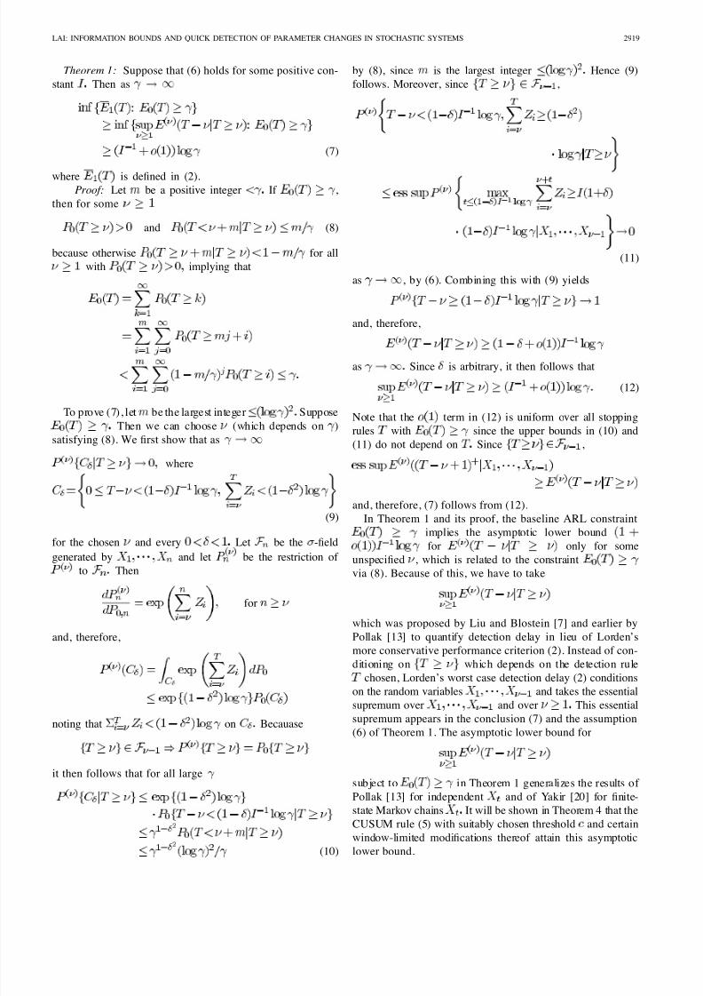
Theorem 1: Suppose that (6) holds for some positive con-
stant Then as
(7)
where is defined in (2).Proof: Let be a positive integer If ,
then for some
and (8)
because otherwise for all
with implying that
To prove (7), let be the largest integer Suppose
Then we can choose (which depends on )
satisfying (8). We first show that as
where
(9)
for the chosen and every Let be the -field
generated by and let be the restriction of
to Then
for
and, therefore,
noting that on Becauase
it then follows that for all large
(10)
by (8), since is the largest integer Hence (9)
follows. Moreover, since ,
(11)
as , by (6). Combining this with (9) yields
and, therefore,
as Since is arbitrary, it then follows that
(12)
Note that the term in (12) is uniform over all stopping
rules with since the upper bounds in (10) and
(11) do not depend on Since ,
and, therefore, (7) follows from (12).
In Theorem 1 and its proof, the baseline ARL constraintimplies the asymptotic lower bound
for only for some
unspecified , which is related to the constraint
via (8). Because of this, we have to take
which was proposed by Liu and Blostein [7] and earlier by
Pollak [13] to quantify detection delay in lieu of Lorden’s
more conservative performance criterion (2). Instead of con-
ditioning on which depends on the detection rule
chosen, Lorden’s worst case detection delay (2) conditions
on the random variables and takes the essential
supremum over and over This essential
supremum appears in the conclusion (7) and the assumption
(6) of Theorem 1. The asymptotic lower bound for
subject to in Theorem 1 generalizes the results of
Pollak [13] for independent and of Yakir [20] for finite-
state Markov chains It will be shown in Theorem 4 that the
CUSUM rule (5) with suitably chosen threshold and certain
window-limited modifications thereof attain this asymptotic
lower bound.

8/4/2019 IEEE Transactions on Information Theory 1998 Lai
http://slidepdf.com/reader/full/ieee-transactions-on-information-theory-1998-lai 4/13
2920 IEEE TRANSACTIONS ON INFORMATION THEORY, VOL. 44, NO. 7, NOVEMBER 1998
B. Information Bounds Under Alternative
Performance Criteria
As pointed out above, Lorden’s asymptotic theory and its
generalization in Theorem 1 give an asymptotic lower bound
for only at the that maximizes the
expected delay. If we want an asymptotic lower bound for
at any given , the proof of Theorem
1 suggests that the baseline ARL constraintshould be replaced by
with but ; see (8).
Indeed, under this probability constraint, we can use the same
arguments as in (9) and (11) to show that
(13)
However, the conditional probability
is difficult to evaluate when the denominator is small. Ignoring
the denominator leads to a simpler probability constraint of the
form We shall require this bound
to hold for all and some that depends only
on , i.e.,
where
but
as (14)
The next theorem gives a uniform (over ) asymptotic lower
bound for under the probability constraint (14)
and the following relaxation of assumption (6): As
(15)
It will be shown later that certain window-limited modifica-
tions of the CUSUM rule (5) attain the asymptotic lower bound
for the detection delay
subject to the probability constraint (14).
Theorem 2: Suppose that (14) and (15) hold for some
positive constant Then as
uniformly in (16)
Proof: For any , define by (9) with re-
placed by Then the same change-of-measure argu-
ment as in (10) shows that for all sufficiently small
by (14), since for all small
Moreover, as in (11), (15) implies that
as Hence
and, therefore,
where the term is uniform in Since
(16) follows.
A Bayesian alternative to the ARL constraint is
the false-alarm probability constraint
(17)
where is a probability measure on the positive integers.
Interpreting as the prior distribution of the change time ,
the left-hand side of (17) is The following theorem,
whose proof is given in the Appendix, gives an asymptoticlower bound for
and shows that the CUSUM rule (5) with suitably chosen
attains the lower bound under certain conditions.
Theorem 3: Suppose that (15) holds for some positive
constant Let be a probability measure on the positive
integers such that as
and
for some positive constant Let be a detection rule
satisfying the probability constraint (17). Then
(18)
Among the three false-alarm constraints (14), (17), and
considered in Theorems 1–3, (14) can be regarded

8/4/2019 IEEE Transactions on Information Theory 1998 Lai
http://slidepdf.com/reader/full/ieee-transactions-on-information-theory-1998-lai 5/13
LAI: INFORMATION BOUNDS AND QUICK DETECTION OF PARAMETER CHANGES IN STOCHASTIC SYSTEMS 2921
as the most stringent. Suppose a detection rule satisfies (14).
Then for and
(19)
Hence if ,
and, therefore,
(20)
Since as Note
that the asymptotic lower bound in Theorem 1 involves
only through From (19), it also follows that
i.e., (17) holds with in place of When
as
since , and the asymptotic
lower bound (18) involves only through In the
sequel we shall therefore focus on the constraint (14), which
is the most stringent among the three false-alarm constraints
discussed above.
C. Window-Limited CUSUM and Moving Average Rules
Let be positive integers such that
but
as (21)
Consider the probability constraint (14). To begin with, sup-
pose the are independent with common density function
for , and common density function for For
the CUSUM rule (1)
for some
for some
(22)
where the second inequality follows from the fact that
has the same distribution under as
and the last inequality is a consequence of
Doob’s submartingale inequality (cf. [17]). Hence
if is so chosen that
When the are not i.i.d. under , the time reversal
argument in (22) breaks down and the CUSUM rule (5)
with need not satisfy (14). To circumvent this
difficulty, we replace in (5) by ,
leading to the window-limited CUSUM rule
(23)
The next theorem, whose proof is goven in the Appendix,
shows that with satisfies (14) and that it
attains the asymptotic lower bound (16) under the condition
(24)
It also shows that under (24) the rules and with suitably
chosen thresholds attain the asymptotic lower bounds fordetection delay in Theorems 1 and 3.
Theorem 4:
i) For the detection rule (23),
If satisfies (21), and (15) and (24) hold for
some then as
uniformly in
ii) If (24) holds for some
and satisfies (21), then
as
and
as
iii) Let be a probability measure on the positive integers
such that
as
Then the Bayesian probability constraint (17) holds for
with
and for with

8/4/2019 IEEE Transactions on Information Theory 1998 Lai
http://slidepdf.com/reader/full/ieee-transactions-on-information-theory-1998-lai 6/13
2922 IEEE TRANSACTIONS ON INFORMATION THEORY, VOL. 44, NO. 7, NOVEMBER 1998
If (24) holds for some and satisfies (21), then
as
The window-limited CUSUM rule (23) with suitably chosenthreshold is therefore asymptotically optimal under the
different performance criteria of Theorems 1–3. Note that (23)
can be written as a composite of moving average rules
where
(25)
The proof of Theorem 4 i) in the Appendix shows that those
with are the most crucial in ensuring the asymptotic
optimality of Moving average rules will be discussed
further at the end of Section IV. In practice, usually involves
unknown parameters that make it impossible to determine
and the optimal window in advance. As will be shown in
the next section, replacing the likelihood ratio statistics (4)
in by mixture or generalized likelihood ratio statistics to
handle unknown parameters leads to detection rules that are
asymptotically as efficient as the window-limited CUSUM
rules which assume knowledge of the unknown parameters.
III. ASYMPTOTICALLY OPTIMAL
COMPOSITE MOVING AVERAGE RULES IN
THE PRESENCE OF UNKNOWN PARAMETERS
In practice, the post-change distribution often involves un-known parameters. Although the setting of a completely
known distribution considered in Section II seems sim-
plistic, the optimal detection theory developed in that setting
provides benchmarks and ideas for the development of de-
tection rules in the presence of unknown parameters. In
particular, suitable modifications of the likelihood ratio sta-
tistics in (25) to handle these unknown parameters
will be shown to provide detection rules that attain the above
asymptotic lower bounds for detection delay.
A. Rules Based on Mixture Likelihood Ratios
Instead of a known conditional density function
for
suppose that one has a parametric family of conditional density
functions so that the baseline distribution
corresponds to the parameter value and the conditional
distribution after the change time corresponds to some other
element of the parameter space As in Section II, we let
denote the case Unlike Section II, the value of
is not assumed to be known. We shall use (instead of
) to denote the probability measure with change time
and changed parameter Let be a probability distribution
on and define the mixture likelihood ratio statistics
Throughout this section we shall let be positive integers
such that
but as (26)
Define the window-limited mixture likelihood ratio rule
(27)
The following lemma shows that with suitably chosen
satisfies the probability constraint (14) and therefore also
(17) and the ARL constraint with
in view of (20).
Lemma 1:
where
Proof: Let be the -field generated by
Since is a nonnegative martingale with
for it follows from Doob’s submartingale
inequality (cf. [17]) that for some
Hence
for some
Let
Assume that under converges in prob-
ability to some positive constant , which we shall denote by
The following theorem, whose proof is given in the
Appendix, shows that attains the asymptotic lower bounds
for detection delay in Theorems 1 and 2 under an assumptionanalogous to (24). Note that since , the
choice of in Lemma 1 satisfies as
Theorem 5: Suppose that for every there exist
and such that and
(28)

8/4/2019 IEEE Transactions on Information Theory 1998 Lai
http://slidepdf.com/reader/full/ieee-transactions-on-information-theory-1998-lai 7/13
LAI: INFORMATION BOUNDS AND QUICK DETECTION OF PARAMETER CHANGES IN STOCHASTIC SYSTEMS 2923
Suppose in (27) satisfies as Then
(29)
uniformly in (30)
B. Window-Limited Generalized Likelihood
Ratio Detection Rules
A more commonly used alternative to the mixture likelihood
ratio statistic for testing versus based on
is the generalized likelihood ratio (GLR) statistic
Replacing by the GLR statistic in
(27) leads to the window-limited GLR rule
(31)
Detection rules of this type were first introduced by Willsky
and Jones [19]. The minimal delay is used to avoid
difficulties with GLR statistics when For example,
if in the case of a normal density with unknown
mean and variance , we need at least two observations to
define uniquely the maximum likelihood estimate of Since
the attainment of the asymptotic lower bounds in Theorems
1–3 by (23) implies that should also attain these asymptotic
lower bounds if and We nextconsider the choice of so that satisfies the probability
constraint (14) which, as pointed out earlier, is the most
stringent of the false alarm constraints in Theorems 1–3.
To analyze the probability in (14) for window-limited GLR
rules, suppose that is a compact -dimensional submanifold
of the Euclidean space and that is twice continuously
differentiable in Let and denote
the gradient vector and Hessian matrix, respectively, and let
denote the interior of It will be assumed that
and belong to For , let be the maximum
likelihood estimate of based on If
then and isnegative definite. This yields the quadratic approximation
when is near , which is commonly used to derive the lim-
iting chi-square distributions of GLR statistics. Let
denote the largest eigenvalue of a symmetric matrix To
ensure that and that is
not too large in a small neighborhood of when triggers
an alarm at time , take and modify as follows:
where
and
(32)
Lemma 2: Assume that is a compact -dimensional
submanifold of and let denote its Lebesgue measure.
Define by (32) with
Then as and (14) holds for all sufficiently
small
The proof of Lemma 2 is given in the Appendix. Examples
and refinements of the window-limited GLR rule, togetherwith simulation studies and recursive algorithms for their
implementation, are given in [5] and [6].
IV. EXAMPLES AND APPLICATIONS
We first discuss the assumptions (6) and (24) in Theorems
1 and 4. Suppose that is a Markov chain with
transition density function for and for
, with respect to some -finite measure on the state
space In this case ,
and (6) and (24) reduce to
for every (33)
Suppose that the transition density function is uniformly
recurrent in the sense that there exist and
a probability measure on such that
(34)
for all measurable subsets and all Then the Markov
chain has a stationary distribution under and (33) holds
with
In particular, assumptions (6) and (24) are satisfied by finite-
state, irreducible chains. Note that assumption (15) in Theo-
rems 2 and 3 is considerably weaker than (6).
Suppose that is the transition density function of a
Markov chain , where assumes the value
before the change time and the value at and after The
parameter space is assumed to be a metric space. Here

8/4/2019 IEEE Transactions on Information Theory 1998 Lai
http://slidepdf.com/reader/full/ieee-transactions-on-information-theory-1998-lai 8/13
2924 IEEE TRANSACTIONS ON INFORMATION THEORY, VOL. 44, NO. 7, NOVEMBER 1998
Suppose that the chain has a stationary distribution under
and
and that (33) (with replaced by holds. Assume
further that
as (35)
where denotes a ball with center and radius From
(35), it follows that
as
Using this together with Markov’s inequality and (33), it
follows that for every , there exists such that (28)holds with noting that in the present Markov
case, (28) reduces to
To fulfill the assumptions of Theorem 5, assume in addition to
(33) and (35) that for every ball centered at
Window-limited GLR rules of the form (31) were introduced
by Willsky and Jones [19] in the context of detecting additive
changes in linear state-space models. Consider the stochastic
system
(36a)
(36b)
in which the unobservable state vector , the input vector ,
and the measurement vector have dimensions and
respectively, and are independent Gaussian vectors with
zero means and The Kalman
filter provides a recursive algorithm to compute the conditional
expectation of the state given the past observations
. The innovations
are independent zero-mean Gaussian vectors with
given recursively by
where
(37)
Suppose at an unknown time the system undergoes some
additive change in the sense that and/or
are added to the right-hand side of (36a) and/or (36b). Then
the innovations are still independent Gaussian vectors with
covariance matrices , but their means are of the
form for instead of the baseline values
for The are matrices that can be evaluated
recursively for when and are specified up to
an unknown parameter (cf. [1, p. 282]). Without assuming
prior knowledge of the parameter and the change time , the
window-limited GLR detector has the form
(38)
where denotes the -dimensional
normal density, , and so that the
matrix whose inverse appears in (38) is nonsingular.
Note that the window-limited GLR rule (38) involves par-
allel recursions, one for each within a moving window. This
can be easily implemented by initializing a new recursion
at every stage while deleting the recursion that has been
initialized at Only those recursions initialized at
are used in the GLR detector (38).
We shall assume that and converge to
and exponentially fast and that the Kalman
filter is asymptotically stable in the sense that defined
in (37) converges exponentially fast to the solution of theRiccati equation
Then
and converges exponentially fast to a limiting matrix
as Under the probability measure associated
with the change time and the parameter ,
(39)
are independent normal random variables with means
and variances for Moreover, converges expo-
nentially fast to
as , and with thus defined, assumption (15) is
satisfied in view of normal tail probability bounds. Since the

8/4/2019 IEEE Transactions on Information Theory 1998 Lai
http://slidepdf.com/reader/full/ieee-transactions-on-information-theory-1998-lai 9/13
LAI: INFORMATION BOUNDS AND QUICK DETECTION OF PARAMETER CHANGES IN STOCHASTIC SYSTEMS 2925
TABLE IAVERAGE RUN LENGTHS OF FOUR DETECTION RULES FOR WITH DIFFERENT WINDOW SIZES
TABLE IIAVERAGE RUN LENGTHS OF THE DETECTION RULES IN TABLE I AT THREE OTHER VALUES OF
are independent, asumption (6) reduces to (15). Similarly, by
independence, assumption (24) reduces in the present setting to
which is clearly satisfied because of normal tail probability
bounds. Therefore, the theory developed in Sections II and III
is applicable to the problem of detecting additive changes in
linear state-space models. As shown in [6], we can choose
as so that (14) holds for the GLR rule
defined in (38) without modifying it as in Lemma 2 for the
general setting. In fact, for linear Gaussian state-space models,
[6, Theorem 1] shows that
as but where is a positive
constant.
Tables I and II report the results of a simulation study of
the performance of the window-limited GLR rule (38) for theproblem of detecting additive changes in the state-space model
where and
are two-dimensional random vectors,
and are independent, zero-mean Gaussian vectors. Here
the in (38) are matrices that can be computedrecursively for as follows:
We set in (38), in which the matrix
is invertible for , and chose three different values of
in this study. The tables consider four different values of thevector of additive changes, resulting in four different values
of It is assumed that the initial state
has the stationary distribution under The threshold is
so chosen that , using Monte Carlo simulations
to evaluate and
The tables show that performs well in detecting changes
with , which is consistent with the asymptotic
theory of developed in [6] showing that attains the
asymptotic lower bounds for detection delay in Theorems
1 and 2 if and as Note in
this connection that in (26) we choose satisfying
so that for fixed and
Instead of taking an inordinately large window
size which is much larger than and for which the
computational complexity of may become unmanageable,
[5] and [6] develop a modification of (38) that is not too
demanding in computational requirements for on-line imple-
mentation and yet is nearly optimal under the performance
criteria of Theorems 1 and 2. The basic idea is to generalize
the Willsky–Jones window to the form
, where with
for some Simulation studies and asymptotic
properties of this modified version of (38) are given in [6].
Tables I and II also study the performance of the window-
limited CUSUM rule defined in (23), which requiresspecification of the vector whose nominal value is chosen
to be in the tables. In Table I, is correctly
specified , and the rule (23) performs well when the
window size satisfies , which is consistent with
Theorem 4 (see condition (21) on the window size). Taking
in (23) yields the CUSUM rule (5). Although the
CUSUM rule (1) has the simple recursive representation
(40)
8/4/2019 IEEE Transactions on Information Theory 1998 Lai
http://slidepdf.com/reader/full/ieee-transactions-on-information-theory-1998-lai 10/13
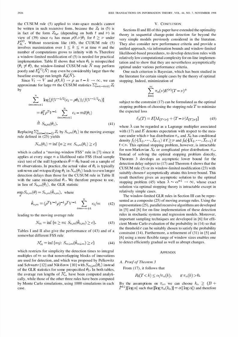
2926 IEEE TRANSACTIONS ON INFORMATION THEORY, VOL. 44, NO. 7, NOVEMBER 1998
the CUSUM rule (5) applied to state-space models cannot
be written in such recursive form, because the in (5) is
in fact of the form (depending on both and ) in
view of (39) since has mean for under
Without recursions like (40), the CUSUM rule (5)
involves maximization over at time and the
number of computations grows to infinity with Therefore
a window-limited modification of (5) is needed for practical
implementation. Table II shows that when is misspecified
, the window-limited CUSUM rule may perform
poorly and may even be considerably larger than the
baseline average run length
Since and as , we can
approximate for large the CUSUM statistics
by
(41)
Replacing by in the moving average
rule defined in (25) yields
which is called a “moving-window FSS” rule in [7] since it
applies at every stage a likelihood ratio FSS (fixed sample
size) test of the null hypothesis based on a sample of
observations. In practice, the actual value of is typically
unknown and misspecifying in leads to even longer
detection delays than those for the CUSUM rule in Table IIwith the same misspecified We therefore propose to use,
in lieu of , the GLR statistic
where
(42)
leading to the moving average rule
(43)
Tables I and II also give the performance of (43) and of a
somewhat different FSS rule
(44)
which restricts for simplicity the detection times to integral
multiples of so that nonoverlapping blocks of innovations
are used for detection, and which was proposed by Pelkowitz
and Schwartz [12] and Nikiforov [10] with instead
of the GLR statistics for some prespecified In both tables,
the average run lengths of have been computed analyti-
cally, while those of the other three rules have been computed
by Monte Carlo simulations, using 1000 simulations in each
case.
V. CONCLUSION
Sections II and III of this paper have extended the optimality
theory in sequential change-point detection far beyond the
very simple models previously considered in the literature.
They also consider new performance criteria and provide a
unified approach, via information bounds and window-limited
likelihood-based procedures, to develop detection rules with
relatively low computational complexity for on-line implemen-tation and to show that they are nevertheless asymptotically
optimal under various performance criteria.
One such criterion is Bayesian, which has been studied in
the literature for certain simple cases by the theory of optimal
stopping. Indeed, minimization of
subject to the constraint (17) can be formulated as the optimal
stopping problem of choosing the stopping rule to minimize
the expected loss
(45)
where can be regarded as a Lagrange multiplier associated
with (17) and denotes expectation with respect to the mea-
sure under which has distribution and has conditional
density if and if
This optimal stopping problem, however, is intractable
for non-Markovian or complicated prior distributions
Instead of solving the optimal stopping problem directly,
Theorem 3 develops an asymptotic lower bound for the
detection delay subject to (17) and Theorem 4 shows that the
CUSUM rule (5) or its window-limited modification (23) with
suitably chosen asymptotically attains this lower bound. This
result therefore gives an asymptotic solution to the optimalstopping problem (45) when , whose exact
solution via optimal stopping theory is intractable except in
relatively simple cases.
The window-limited GLR rules in Section III can be repre-
sented as a composite (25) of moving average rules. Using the
representation (25), parallel recursive algorithms are developed
in [5] and [6] for on-line implementation of these detection
rules in stochastic systems and regression models. Moreover,
important sampling techniques are developed in [6] for effi-
cient Monte Carlo evaluation of the probability in (14) so that
the threshold can be suitably chosen to satisfy the probability
constraint (14). Furthermore, a refinement of (31) in [5] and
[6] using a more flexible range of window sizes enables oneto detect efficiently gradual as well as abrupt changes.
APPENDIX
A. Proof of Theorem 3
From (17), it follows that
if
By the assumptions on we can choose
such that and therefore

8/4/2019 IEEE Transactions on Information Theory 1998 Lai
http://slidepdf.com/reader/full/ieee-transactions-on-information-theory-1998-lai 11/13
LAI: INFORMATION BOUNDS AND QUICK DETECTION OF PARAMETER CHANGES IN STOCHASTIC SYSTEMS 2927
Hence for
(46)
Define by (9) with replaced by Then as in
(10), for sufficiently small
by (46). Moreover, from (15), it follows as in (11) that
as Hence
so
noting that By (17),
as
Since
it then follows that
Since can be arbitrarily small, (18) follows.
B. Proof of Theorem 4
We first prove part ii) of the theorem. Let be the -fieldgenerated by Clearly, and therefore
To prove that define the stopping times
and
for Let Then on
for some (47)
by Doob’s submartingale inequality and the optional sampling
theorem (cf. [17]), since is a
nonnegative martingale under with mean (see also (51)
below). Let
and
for some
Then
by (47), and, therefore,
Since
it then follows that
To prove that when (21) and (24)
hold and , it suffices to show that for any
such that (see (21))
(48)
as Let be the largest integer
By (24)
(49)
for all large Since and lim inf , it
follows that for all sufficiently small
for any and , as can be shown by applying
(49) and conditioning on for
in succession (in view of the property

8/4/2019 IEEE Transactions on Information Theory 1998 Lai
http://slidepdf.com/reader/full/ieee-transactions-on-information-theory-1998-lai 12/13
2928 IEEE TRANSACTIONS ON INFORMATION THEORY, VOL. 44, NO. 7, NOVEMBER 1998
if is a sub- - field of ). Hence for all
sufficiently large
(50)
implying (48) sinceWe next prove part i) of the theorem. From (23) it follows
that
for some
As in (47), it follows from Doob’s submartingale inequality
(cf. [17]) that for every
(51)
Hence
for all and, therefore, (14) holds if For
this choice of , since (14) and (15) hold, (16) holds with
replaced by Moreover,
since under (21). Hence, under (24), (48)
holds for all sufficiently small , from which it follows
that as
uniformly in (52)
since
To prove part iii) of the theorem, first note that
and that (52) yields
as
since
As in (19), we have
by part i) of the theorem. Hence
Similarly,
follows from
for some
where the last inequality follows from (51).
C. Proof of Theorem 5
The proof of (29) is similar to that of (50), noting that
Moreover, as in the derivation of (52), (30) follows from (29).
D. Proof of Lemma 2
First note that
where
To analyze , we use a change-of-measure
argument. Let denote the probability measure under
which the conditional density of given is
for and is for
Define a measure Since is
compact and therefore has finite Lebesgue measure, is
a finite measure. For , the Radon–Nikodym derivative
of the restriction of to relative to the restriction of to is
Hence by Wald’s likelihood ratio identity (cf. [16])
(53)

8/4/2019 IEEE Transactions on Information Theory 1998 Lai
http://slidepdf.com/reader/full/ieee-transactions-on-information-theory-1998-lai 13/13
LAI: INFORMATION BOUNDS AND QUICK DETECTION OF PARAMETER CHANGES IN STOCHASTIC SYSTEMS 2929
For , if , then and,
therefore, by Taylor’s theorem
where for some Hence if
and , then
as Therefore, by the definition of and (53),
Since
(14) holds for all small if the threshold for is chosen
as in Lemma 2.
REFERENCES
[1] R. K. Bansal and P. Papantoni-Kazakos, “An algorithm for detectinga change in a stochastic process,” IEEE Trans. Inform. Theory, vol.
IT-32, pp. 227–235, Mar. 1986.[2] M. Basseville and I. V. Nikiforov, Detection of Abrupt Changes. Theory
and Applications. Englewood Cliffs, NJ: Prentice-Hall, 1993.[3] T. Bojdecki, “Probability maximizing approach to optimal stopping and
its application to a disorder problem,” Stochastics, vol. 3, pp. 61–71,
1979.
[4] T. L. Lai, “Asymptotic optimality of invariant sequential probabiity ratiotests,” Ann. Statist., vol. 9, pp. 318–333, 1981.
[5] , “Sequential changepoint detection in quality control and dy-namical systems,” J. Roy. Statist. Soc. Ser. B, vol. 57, pp. 613–658,
1995.[6] T. L. Lai and J. Z. Shan, “Efficient recursive algorithms for detection of
abrupt changes in signals and control systems,” IEEE Trans. Automat.
Contr., vol. 44, May 1999, to be published.[7] Y. Liu and S.D. Blostein, “Quickest detection of an abrupt change in a
random sequence with finite change-time,” IEEE Trans. Inform. Theory,vol. 40, pp. 1985–1993, Nov. 1994.
[8] G. Lorden, “Procedures for reacting to a change in distribution,” Ann.
Math. Statist., vol. 42, pp. 1897–1908, 1971.[9] G. Moustakides, “Optimal procedures for detecting changes in distribu-
tions,” Ann. Statist., vol. 14, pp. 1379–1387, 1986.[10] I. V. Nikiforov, “Two strategies in the problem of change detection and
isolation,” IEEE Trans. Inform. Theory, vol. 43, pp. 770–776, Mar. 1997.[11] E. S. Page, “Continuous inspection schemes,” Biometrika, vol. 41, pp.
100–115, 1954.[12] L. Pelkowitz and S. C. Schwartz, “Asymptotically optimum sample
size for quickest detection,” IEEE Trans. Aerosp. Electron. Syst., vol.AES-23, pp. 263–272, Mar. 1987.
[13] M. Pollak, “Optimal detection of a change in distribution,” Ann. Statist.,vol. 13, pp. 206–227, 1985.
[14] Y. Ritov, “Decision theoretic optimality of the CUSUM procedure,”
Ann. Statist., vol. 18, pp. 1464–1469, 1990.[15] A. N. Shiryayev, Optimal Stopping Rules. New York: Springer-Verlag,
1978.[16] D. Siegmund, Sequential Analysis: Tests and Confidence Intervals.
New York: Springer-Verlag, 1985.[17] D. Williams, Probability with Martingales. Cambridge, U.K.: Cam-
bridge Univ. Press, 1991.[18] A. S. Willsky, “A survey of design methods for failure detection in
dynamic systems,” Automatica, vol. 12, pp. 601–611, 1976.[19] A. S. Willsky and H. L. Jones, “A generalized likelihood ratio approachto detection and estimation of jumps in linear systems,” IEEE Trans.
Automat Contr., vol. AC-21, pp. 108–112, Feb. 1976.[20] B. Yakir, “Optimal detection of a change in distribution when the obser-
vations form a Markov chain with a finite state space,” in Change-Point
Problems, E. Carlstein, H. Muller, and D. Siegmund, Eds. Hayward,
CA: Inst. Math. Statist., 1994, pp. 346–358.