IEEE TRANSACTIONS ON INDUSTRIAL ELECTRONICS 1 Adaptive ...

0278-0046 (c) 2016 IEEE. Personal use is permitted, but republication/redistribution requires IEEE permission. See http://www.ieee.org/publications_standards/publications/rights/index.html for more information.

This article has been accepted for publication in a future issue of this journal, but has not been fully edited. Content may change prior to final publication. Citation information: DOI 10.1109/TIE.2017.2674581, IEEETransactions on Industrial Electronics

IEEE TRANSACTIONS ON INDUSTRIAL ELECTRONICS 1

Adaptive Dynamic Programming-Based OptimalControl Scheme for Energy Storage Systems With

Solar Renewable EnergyQinglai Wei, Member, IEEE, Guang Shi, Ruizhuo Song, Member, IEEE, and Yu Liu

Abstract— In this paper, a novel optimal energy storage controlscheme is investigated in smart grid environments with solarrenewable energy. Based on the idea of adaptive dynamicprogramming (ADP), a self-learning algorithm is constructed toobtain the iterative control law sequence of the battery. Based onthe data of the real-time electricity price (electricity rate in brief),the load demand (load in brief), and the solar renewable energy(solar energy in brief), the optimal performance index function,which minimizes the total electricity cost and simultaneouslyextends the battery’s lifetime, is established. A new analysismethod of the iterative ADP algorithm is developed to guaranteethe convergence of the iterative value function to the optimumunder iterative control law sequence for any time index in aperiod. Numerical results and comparisons are presented toillustrate the effectiveness of the developed algorithm.

Index Terms— Adaptive critic designs, adaptive dynamic pro-gramming, approximate dynamic programming, solar renewableenergy, energy storage system, optimal control, energy storage.

I. INTRODUCTION

ALONG with the development of smart grid, more andmore intelligence has been required in the design of

smart energy storage systems [1]–[3]. Energy storage systemsof the future will provide end users a better energy manage-ment, reducing waste and advanced optimization technology.Renewable energies, electricity load, and energy storage e-quipments (battery) can be defined as smart energy storagesystems which are able to operate with physically islanded[4], [5]. The intelligent optimal utilization of energy storage,along with the development of computational intelligences, hasreceived much attention in recent years [6]–[8].

Adaptive dynamic programming (ADP) is an important andpowerful brain-like intelligent optimal control method [9]–[20], due to its strong abilities of self-learning and adaptivity,and has widely been applied to obtain the optimal control forenergy storage systems [21]–[24]. In [25], an action-dependentheuristic dynamic programming (ADHDP) algorithm, which is

This work was supported in part by the National Natural Science Foun-dation of China under Grants 61374105, 61533017, 61273140, 61673054,61503379, and 61233001.

Q. Wei and G. Shi are with The State Key Laboratory of Management andControl for Complex Systems, Institute of Automation, Chinese Academyof Sciences, Beijing 100190, China and also with the University of ChineseAcademy of Sciences, Beijing 100049, China. (phone: +86-10-82544517; fax:+86-10-82544799; emails: [email protected], [email protected]).

R. Song is with the School of Automation and Electrical Engineering,University of Science and Technology Beijing, Beijing 100083, China (email:[email protected], [email protected]).

Y. Liu is with Institute of Automation, Chinese Academy of Sciences,Beijing 100190, China (e-mail: [email protected]).

also called Q-learning algorithm [26], was proposed to obtainthe optimal energy storage (battery) control law in achievingminimization of the cost through neural network learning.In [27], a time-based Q-learning algorithm was proposed toobtain the optimal battery control law to minimize the totalelectricity cost for energy storage systems, where the wind andsolar energies were taken into consideration. In [28], a particleswarm optimization (PSO) algorithm was introduced to pre-train the weights of the neural networks, which speeds up thetraining of neural networks in ADP. In [29], a new event-triggered ADP algorithm was proposed to obtain the optimalfrequency control law of the load.

In previous ADP algorithms for energy storage systems,however, it is mainly focused on the structure improvements,while the properties of the proposed ADP structures areseldom analyzed. In this case, the optimality of the achievedcontrol scheme cannot be guaranteed. Second, the previousADP algorithms required that the time index t reach infinity toobtain the optimal performance index function, which meansthat the optimal performance index function and optimalcontrol law are time-invariant functions as t → ∞. As theelectricity rate, the load demand, and the solar renewableenergy are generally time-variant functions, the convergedtime-invariant functions cannot effectively approximate theoptimal performance index function and optimal control lawof the energy storage systems. In [30], without consideringthe renewable energy, a dual iterative Q-learning algorithmof ADP was proposed to obtain the optimal battery controlpolicy for energy storage systems, where it was proven thatthe iterative Q function is convergent to the optimum, as theiteration index increases to infinity. Considering the renewableenergy, it presents a more complex scheme comparing with[30], where the optimal decisions for the power flows shouldcover all the possibilities for the renewable energy resource,the load, and the battery. Hence, the ADP algorithm andthe property analysis in [30] cannot directly be applied toenergy storage systems with renewable energy. A new ADPalgorithm with new property analysis methods is necessary forthe optimal battery control of the energy storage systems withrenewable energy. This motivates our research.

In this paper, inspired by [25], [27], [30], a new iterativeADP algorithm is developed to obtain the optimal battery con-trol for energy storage systems with solar renewable energy.According to the data of the electricity rate, the load, and thesolar energy, the energy storage system is described and theoptimization objective is established. Based on the established




system, the iterative ADP algorithm is implemented, where ineach iteration, an iterative control law sequence of a period isobtained instead of a single control law. Next, the propertiesof the iterative ADP algorithm are analyzed. As the iterationindex increases to infinity, we emphasize that the iterativevalue function for any time index in the period is proven toconverge to the optimal performance index function. Finally,numerical experiments and comparisons are presented to showthe effectiveness of the iterative ADP algorithm.

II. PRELIMINARIES AND ASSUMPTIONS

In this section, the energy storage system with renewableenergy, i.e., solar energy, is described and the optimizationobjective of our research will be defined.

A. NotationThe list of used notations is reported as follows.k, t Time indices.i, j Iteration indices.zb,k Battery energy (kWh).zmin

b /zmaxb Minimum/maximum storage energy of

the battery (kWh).ϑ(·) Charging/discharging efficiency of battery.Trate Rated charing/discharging power of the

battery (kW).TG,k Power supply of the grid (kW).TL,k Power of the load (kW).TR,k Power of the renewable resource (kW).TRL,k Power from the renewable resource to the

load (kW).TRB,k Power from the renewable resource to the

battery (kW).TGL,k Power from the power grid to the load

(kW).TGB,k Power from the power grid to the

battery (kW).TBL,k Power from the battery to the load (kW).λ Periods of the load, electricity rate, and

the renewable resource.GHIk Global horizontal irradiance received on a

horizontal surface (kWh/m2).ϑpv the efficiency of the PV.Apv the total area of the PV panel (m2).Ck Electricity rate (cents/kWh).zo

b Middle of storage limit (kWh).α, β, δ Given positive constants in performance

index function.γ Discount factor.xk System state.uk Control input.uk Control law sequence from k to ∞.Uk Control sequence in a period.U(·) Control law sequence in a period.F (·), F (·) System functions.L (·), U (·) Utility functions.J(·) Performance index function.V ji (·) Iterative value function.

Ψ(·) Initial iterative value function.

B. Energy Storage System With Solar Renewable Energy

The energy storage system with solar renewable energyis described in [27], [28], which is shown in Fig. 1. It iscomposed of the power grid, the solar renewable energy (solarenergy in brief) resource, the load demand (load in brief), andthe battery system. In the energy storage system, the solar

Renewable

EnergyGrid Battery

Power Management Unit

Load

Unidirectional

Power Flow

Unidirectional

Power Flow

Unidirectional

Power Flow

Bidirectional

Power Flow

Fig. 1. Energy storage system with solar energy

energy can (i) meet the load; (ii) charge the battery. The batterycan (i) charge from the grid; (ii) charge from solar energyresource; (iii) discharge to meet the load; (iv) idle. There arethree power flows to meet the load, including the power grid,the renewable resource, and the battery, where the load balancecan be defined as

TL,k = TRL,k + TGL,k + TBL,k. (1)

The balance of the power grid can be defined as

TG,k = TGL,k + TGB,k. (2)

In this paper, the renewable energy, i.e., solar energy, isconsidered. The power of the solar energy depends on positionof the sun in the sky and hence the estimated total solar energyvaries in each hour of a day. A typical solar panel characteristicis chosen as in [27], [28], [31]. The solar energy in first weekof August 2014 in San Francisco is shown in Fig. 2(a). Theaverage solar energy in a day is shown in Fig. 2(b). The power

20 40 60 80 100 120 140 160

Time (Hours)(a)

0

0.2

0.4

0.6

0.8

1

Sol

ar e

nerg

y (k

W)

2 4 6 8 10 12 14 16 18 20 22 24

Time (Hours)(b)

0

0.2

0.4

0.6

0.8

1

Sol

ar e

nerg

y (k

W)

Fig. 2. Solar energy in San Francisco. (a) Solar energy in 168 hours. (b)Average solar energy in a day.

output for a photovoltaic (PV) panel [27], [32] at k = 0, 1, . . .can be expressed as TR,k = GHIk · ϑpv · Apv, where ϑpv isincluded in the range [ 0, 1]. In this paper, as the solar energy




can meet the load and charge the battery, the energy balanceof the solar energy can be expressed as

TR,k = TRL,k + TRB,k. (3)

C. Battery Model

The battery model used in this work is based on [25],[33], [34], where battery efficiency is considered to extendthe battery’s lifetime as far as possible. Under the situationthat the battery cannot charge and discharge simultaneously,the battery model can be expressed as

zb,k+1 =zb,k − TBL,k(0.898− 0.173TBL,k/Trate)+ (TRB,k + TGB,k)(0.898− 0.173(TRB,k

+ TGB,k)/Trate). (4)

In this paper, for the convenience of analysis, the battery self-discharge is not considered. The storage limits are defined asfollowing

zminb ≤ zb,k ≤ zmax

b . (5)

D. Assumptions and Optimization Objectives

For convenience of analysis, results of this paper are basedon the following assumptions.

Assumption 1: The power flow from the energy storagesystem to the grid is not permitted.

Assumption 2: The electricity rate, the load, and the solarenergy are periodic functions with the period λ = 24 hours.

From Assumption 1, we can get TBL,k ≥ 0. According toAssumption 2, the parameters Ck, TL,k, and TR,k satisfy

Ck = Ck+λ, TL,k = TL,k+λ, TR,k = TR,k+λ. (6)

Inspired by [30], the performance index function, which isexpected to be minimized, is expressed as

∞∑k=0

γk(α(CkTGL,k)

2 + β(zb,k −zob)

2

+ δ(TRB,k + TGB,k − TBL,k)2), (7)

where zob = 1

2 (zminb +zmax

b ) is the middle of storage limit.The first term of the performance index function aims tominimize the total cost from the grid. The second term avoidsfully charging/discharging of the battery and the third term isto prevent large charging/discharging power of the battery.

III. ITERATIVE ADP ALGORITHM FOR ENERGY STORAGESYSTEMS WITH SOLAR ENERGY

In this section, a novel iterative ADP algorithm is developed,which aims to maintain the energy storage systems at theoptimum operating point under the solar energy.

A. System Establishment and Algorithm Derivations

As the solar energy is cost free, the energy of the renewableresource, first and foremost, is desired to meet the load andthe rest of the energy is desired to charge the battery. Thus,we can derive that

TRL,k =

{TR,k, TL,k − TR,k ≥ 0,TL,k, TL,k − TR,k < 0,

(8)

and

TRB,k =

{0, TL,k − TR,k ≥ 0,

TR,k − TL,k, TL,k − TR,k < 0.(9)

According to (2) and (9), the load balance (1) can berewritten as PL,k = TG,k + (TBL,k −TGB,k). The renewableenergy to charge the battery is PR,k = TR,k − TL,k forTR,k − TL,k ≥ 0, and PR,k = 0 for TR,k − TL,k < 0.For convenience of analysis, we introduce delays in PL,k,TBL,k and TGB,k. Then, we can define the load balance asPL,k−1 = TG,k + TBL,k−1 − TGB,k−1. Let x1,k = TG,k

and x2,k = zb,k − zob be the two system states. From the

model of the battery, we know that the power flows TGB,k,and TBL,k are nonnegative values, i.e., TGB,k ≥ 0 andTBL,k ≥ 0. As the battery is not permitted to charge anddischarge simultaneously, we know TBL,k = 0, if TGB,k ≥ 0and TGB,k = 0, if TBL,k ≥ 0. Then, we can define the controlinput as uk = TBL,k − TGB,k. Letting xk = [x1,k, x2,k]

T, theequation of the energy storage system can be written as

xk+1 = F (xk, uk, k)

=

(PL,k − uk

x2,k − (uk − PR,k)ϑ(uk − PR,k)

), (10)

where ϑ(uk −PR,k) = 0.898− 0.173|uk −PR,k|/Trate. Letuk = (uk, uk+1, . . .) denote the control sequence from k to

∞. Let Mk =

[αC2

k 00 β

]and let x0 be the initial state.

According to the definitions of the states and controls, theperformance index function can be written as J(x0, u0, 0) =∞∑k=0

γkL (xk, uk, k), and the optimal performance index func-

tion satisfies the following Bellman equation

J∗(xk, k) = infuk

{L (xk, uk, k) + γJ∗(xk+1, k + 1)

}, (11)

where L (xk, uk, k) = xTkMkxk + δu2

k.In the following, the detailed derivations of the iterative

ADP algorithm is presented. First, according to (10), for j =0, 1, . . . λ− 1, we define a new system as

xk+1 = F (xk, uk, j)

=

(PL,λ−1−j − uk

x2,k − (uk − PR,λ−1−j)ϑ(uk − PR,λ−1−j)

).

(12)

For j = 0, 1, . . . , λ− 1, we let

U (xk, uk, j) = xTkMλ−1−jxk + δu2

k, (13)

where Mλ−1−j =

[α(Cλ−1−j)

2 00 β

]. Let the initial itera-

tive value function Ψ(xk) be an arbitrary positive semi-definitefunction. For i = 0, 1, . . . and j = 0, 1, . . . , λ− 1 be iteration




indices. For i = 0 and j = 0, the initial iterative value functionis defined as V 0

0 (xk) = Ψ(xk). Then, for j = 0, 1, . . . , λ− 1,the iterative control law is obtained by

vj0(xk) = argminuk

{U (xk, uk, j) + γV j0 (xk+1)}, (14)

where xk+1 = F (xk, uk, j) is defined in (12) and the utilityfunction U (xk, uk, j) is defined in (13). According to theiterative control law vj0(xk), we can update the iterative valuefunction by

V j+10 (xk) = U (xk, v

j0(xk), j) + γV j

0 (F (xk, vj0(xk), j)).

(15)

For i = 1, 2, . . ., we let V 0i (xk) = V λ

i−1(xk). Then, fori = 1, 2, . . ., j = 0, 1, . . . , λ − 1, the iterative control lawis obtained by

vji (xk) = argminuk

{U (xk, uk, j) + γV ji (xk+1)}, (16)

and the iterative value function is updated by

V j+1i (xk) = U (xk, v

ji (xk), j) + γV j

i (F (xk, vji (xk), j)).

(17)

Then, for any i = 0, 1, . . . and j = 0, 1, . . . , λ − 1, we canconstruct the periodic iterative control law sequence by

Uji (xk) =

{vji (xk), v

j−1i (xk), . . . , v

0i (xk), v

λ−1i (xk),

vλ−2i (xk), . . . , v

j+1i (xk)

}. (18)

Remark 1: The developed iterative ADP algorithm (14)–(17) possesses inherent differences comparing with the it-erative Q-learning algorithm in [30]. First, in [30], withoutconsidering the solar energy, the iterative Q-learning algorithmwas developed to obtain the optimal battery control for theenergy storage system. In this paper, the solar energy is clearlyconsidered in the iterative ADP algorithm (14)–(17), whichdisplays a more complex system. Second, in [30], the iterativeQ function, which contains both state and control information,was constructed. In this paper, the iterative value functionV ji (xk) is only the function of state. Hence, the computation

quantity for updating the iterative value function is smallerthan the iterative Q function in [30]. Third, in [30], it wasrequired that the time index satisfied k ∈ {0, λ, 2λ, . . .}to construct the Q-learning algorithm, while in this paper,the time index is k = 0, 1, . . .. Furthermore, in [30], theproperties of the iterative Q function for k ∈ {0, λ, 2λ, . . .}were analyzed, which lacked analyzing the properties forother time index. Thus, we say that the analysis in [30] isnot complete and may not be applicable. For the developediterative ADP algorithm in this paper, a new analysis methodwill be presented.

B. Property Analysis

In this subsection, the properties of the iterative ADPalgorithm (14)–(17) will be analyzed. It will be shown thatthe iterative value function will converge to the optimum asthe iteration index increases to infinity. First, we will analyzethe property of the optimal performance index function. It will

be shown that the optimal performance index function is aperiodic function under the assumptions in this paper.

Theorem 1: If Assumptions 1–2 hold, then for any statexk, k = 0, 1, . . ., the optimal performance index functionJ∗(xk, k) satisfies

J∗(xk, k) = J∗(xk, k + λ). (19)The proof of Theorem 1 is shown in Appendix I. From

Theorem 1, we know that the optimal performance indexfunction is a periodic function with the period λ = 24.Next, the convergence of the iterative value function will beanalyzed. It will be proven that the iterative value functionconverges to the optimum as the iteration index increases toinfinity.

Theorem 2: For i = 0, 1, . . . and j = 0, 1, . . . , λ − 1, letV j+1i (xk) and vji (xk) be obtained by (14)–(17). If Assump-

tions 1–2 holds, then for any j = 0, 1, . . . , λ− 1, the iterativevalue function V j+1

i (xk) converges to its optimal performanceindex function as i → ∞, which satisfies

limi→∞

V j+1i (xk) = J∗(xk, λ− j − 1). (20)

The proof of Theorem 2 is shown in Appendix II.

IV. NUMERICAL EXPERIMENTS

In this section, numerical experiments and comparisons willbe displayed to show the performance of the iterative ADPalgorithm. The profiles of the real-time electricity rate and theload are chosen from ComEd Company in [35] and NAHBResearch report in [36], respectively. The trajectories of theelectricity rate and the load in 168 hours (one week) are shownin Figs. 3(a) and (c), respectively. The average trajectoriesof the electricity rate and the load are shown in Figs. 3(b)and (d), respectively. In this paper, the average electricity rate,average load, and average solar energy are used as the periodicfunctions with the period λ = 24 to implement the iterativeADP algorithm.

0 50 100 1501.5

2

2.5

3

3.5

4

4.5

Time (Hours)(a)

Rat

e (c

ents

/kW

h)

0 5 10 15 20 251.5

2

2.5

3

3.5

4

4.5

Time (Hours)(b)

Rat

e (c

ents

/kW

h)

0 50 100 1500.5

1

1.5

2

Time (Hours)(c)

Load

(kW

)

0 5 10 15 20 250.5

1

1.5

2

Time (Hours)(d)

Load

(kW

)

Fig. 3. Electricity rate and load power. (a) Electricity rate for 168 hours.(b) Average electricity rate. (c) Load for 168 hours. (b) Average load.

Choose the capacity of the battery as 16 kWh. The ratedpower of the battery is 3 kW. Let the lower and upper storagelimits of the battery be zmin

b = 2 kWh and zmaxb = 14

kWh, respectively. Let γ = 0.95. The initial level of thebattery is 9 kWh. Let the performance index function beexpressed as in (7), where we set α = 1, β = 0.3 and




δ = 0.2. Choose the initial function as Ψ(xk) = xTkPxk,

where P = [2.05, 0.11; 0.11, 8.07]. Let the initial state bex0 = [1, 9]T. After normalizing the data of the electricityrate, the load, and the solar energy [26], we implement thedeveloped iterative ADP algorithm for i = 15 iterations tomake the iterative value function convergent. The simulationplots of the iterative value function V j

i (xk) for i = 0, 1, . . . , 15and j = λ − 1 are shown in Fig. 4. The trajectory of theiterative value function V j

i (xk) at x0 is shown in Fig. 5. Fromthe simulation results, for any j = 0, 1, . . . , λ−1, the iterativevalue function is convergent after 15 iterations, which justifiesthe correctness of the developed algorithm.

Fig. 4. The plots of the iterative value function V ji (xk) for i = 0, 1, . . .

and j = λ− 1

0

5

10

15

20

25

0

5

10

15

4

5

6

7

8

9

10

11

ji

Itera

tive

valu

e fu

nctio

n

Fig. 5. The trajectory of the iterative value function V ji (xk) at x0

After i = 15 iterations, the optimal battery control law forthe energy storage system is achieved. The optimal batterycontrol in 168 hours is shown in Fig. 6. The plot of theoptimal battery energy is shown in Fig. 7. From Figs. 6 and7, for different time indices, the optimal battery control lawis different and the optimal charging/discharging power of thebattery at each hour is obtained.

To show the superiority of the developed iterative ADPalgorithm, three traditional optimal control methods, includingtime-based Q-learning (TBQL) algorithm [25], [26], particleswarm optimization (PSO) algorithm [28] and model predic-tive control (MPC) algorithm [37], [38], are employed fornumerical comparisons. In the TBQL algorithm [25], [26], fork = 1, 2, . . ., the iterative control law is designed to satisfythe following optimality equation

Q(xk−1, uk−1, k − 1) = U(xk, uk, k) +Q(xk, uk, k). (21)

20 40 60 80 100 120 140 160−1.5

−1

−0.5

0

0.5

1

1.5

2

Time (Hours)

Opt

imal

bat

tery

cha

rgin

g/di

scha

rgin

g po

wer

(kW

)

Fig. 6. Optimal battery control with solar energy

20 40 60 80 100 120 140 1600

2

4

6

8

10

12

14

Time (Hours)

Bat

tery

Ene

rgy

(kW

h)

Fig. 7. Optimal battery energy in 168 hours

We implement the TBQL for 150 time steps, which makes theQ function converge.

In PSO algorithm [28], the movement of each particlenaturally evolves to an optimal or near-optimal solution. Let Gbe the swarm size. The position of each particle is representedby xℓ

k, ℓ = 1, 2, . . . ,G and its movement by the velocity vectorvℓk. Then, the update rule of PSO can be expressed as

xℓk = xℓ

k−1 + νℓk

νℓk = ωνℓk−1 + rand1ρT1 (p

ℓ − xℓk−1) + rand2ρ

T2 (pg − xℓ

k−1).(22)

Choose the swarm size G = 30. Let the inertia factor be ω =0.7. Let the correction factors ρ1 = ρ2 = [1, 1]T . Let rand1and rand2 be random numbers in [0, 1]. Let pℓ be the bestposition of particles and let pg be the global best position. Weimplement the PSO algorithm for 120 iterations, which makesthe performance index function minimized.

Within the MPC framework [37], [38], it is to solve theoptimization problem at the current time step k = 0, 1, . . ..In the MPC, the receding horizon control algorithm [38] isemployed to obtain the optimal battery control law. For k =0, 1, . . ., the finite horizon value function is expressed as

V (xk, k) =k+T∑τ=k

γτL (xτ , uτ , τ), (23)

where we let γ = 0.95 and T = 20. In each receding horizon,the shooting method and sequential quadratic programming[39] are used to obtain the current optimal control law, wherethe terminal value function is set as V (xk+T , k + T ) = 0.




Based on the TBQL, PSO, MPC and the iterative ADPalgorithm, the comparisons of the power supply from the gridis shown in Fig. 8(a). The comparisons of the battery powersupply is shown in Fig. 8(b). The battery charging power andthe real-time cost comparisons for TBQL, PSO, MPC andthe iterative ADP algorithm are shown in Figs. 8(c) and (d),respectively.

0 50 100 150

Time (Hours)(a)

0

0.5

1

1.5

2

2.5

Pow

er s

uppl

y fr

om g

rid (

kW)

Iterative ADP TBQL MPC PSO

0 50 100 150

Time (Hours)(b)

0

0.5

1

1.5

Pow

er s

uppl

y fr

om b

ater

y (k

W)


0 50 100 150

Time (Hours)(c)

-1.5

-1

-0.5

0

Bat

tery

cha

rgin

g po

wer

(kW

)


0 50 100 150

Time (Hours)(d)

0

2

4

6

8

Rea

l-tim

e co

st (

cent

s)

Original Iterative ADP TBQL MPC PSO

Fig. 8. Simulation comparisons. (a) Power supply from the grid. (b) Powersupply from the battery. (c) Charging power of the battery. (b) Real-time cost.

From Figs. 8(a)–(d), when the electricity rate and the loaddemand are low, comparing with TBQL, PSO and MPCalgorithms, the iterative ADP algorithm reaches the maximumpower supply from the grid to charge the battery. When theelectricity rate and the load demand are high, the iterativeADP algorithm supplies the maximum battery power to meetthe load demand and thus, iterative ADP algorithm reachesthe minimum real-time cost comparing with TBQL, PSO andMPC algorithms. On the other hand, when the solar energyis high, it directly meet the load demands, which preventsthe power from the grid and the battery. Using the iterativeADP algorithm, the grid and battery supply powers are theminimium when the solar energy is high, comparing withTBQL, PSO and MPC algorithms. Thus, using the iterativeADP algorithm, the minimum cost can be achieved. Thetotal cost comparisons of the TBQL, PSO, MPC, and theiterative ADP algorithm are shown in Table I, which verifiesthe superiority of the developed ADP algorithm.

TABLE ICOST COMPARISON

Original TBQL PSO MPC Iterative ADPTotal cost (cents)in San Francisco 682.46 454.32 477.99 467.93 441.27

Saving (%) 33.48 30.01 31.49 35.43Total cost (cents)

in Boston 459.19 474.14 465.34 438.95Saving (%) 32.72 30.52 31.81 35.68

Now, we choose solar energy in first week of August 2014in Boston [27], [28] to verify the effectiveness of the iterativeADP algorithm. The solar energy in a week is shown in Fig.9(a) and the average one is displayed in Fig. 9(b). Let the rate

and load data be the same as in Figs. 3(a) and (c), respectively.Implementing the iterative ADP algorithm for 15 iterations,such that the iterative value function converges to the optimum.The plots of the optimal battery control and optimal batteryenergy are shown in Fig. 9(c) and (d), respectively, where theoptimal battery control law can be achieved. TBQL, PSO, andMPC methods are also employed for comparisons. Based onthe new solar energy, the comparisons of the power supplyfrom the grid is shown in Fig. 10(a). The comparisons ofthe battery power supply is shown in Fig. 10(b). The batterycharging power and the real-time cost comparisons for TBQL,PSO, MPC and the iterative ADP algorithm are shown inFigs. 10(c) and (d), respectively. It can be seen that whenthe electricity rate and the load demand are low, the iterativeADP algorithm reaches the maximum power supply to chargethe battery comparing with TBQL, PSO and MPC algorithms.The grid and battery supply powers are the minimium usingthe iterative ADP algorithm, when the solar energy is high.The total cost comparisons of the TBQL, PSO, MPC, and theiterative ADP algorithm under the new solar energy are shownin Table I, which can verify the superiority of the developedADP algorithm.

20 40 60 80 100 120 140 160

Time (Hours)(a)

0

0.2

0.4

0.6

0.8

1

Sol

ar e

nerg

y (k

W)

5 10 15 20

Time (Hours)(b)

0

0.2

0.4

0.6

0.8

1

Sol

ar e

nerg

y (k

W)

20 40 60 80 100 120 140 160

Time (Hours)(c)

-1.5

-1

-0.5

0

0.5

1

1.5

Bat

tery

cha

rgin

g/di

scha

rgin

g po

wer

(kW

)

20 40 60 80 100 120 140 160

Time (Hours)(d)

0

2

4

6

8

10

12

Bat

tery

ene

rgy

(kW

h)

Fig. 9. Solar energy in Boston and control results. (a) Solar energy inBoston. (b) Average solar energy. (c) Optimal battery control. (d) Optimalbattery energy.

0 50 100 150

Time(Hours)(a)

0

0.5

1

1.5

2

2.5

Pow

er s

uppl

y fr

om g

rid (

kW)


0 50 100 150

Time(Hours)(b)

0

0.5

1

1.5

Pow

er s

uppl

y fr

om b

ater

y (k

W)

Iterative ADP PSO MPC TBQL

0 50 100 150

Time(Hours)(c)

-1.5

-1

-0.5

0

Bat

tery

cha

rgin

g po

wer

(kW

)


0 50 100 150

Time(Hours)(d)

0

2

4

6

8

Rea

l-tim

e co

st (

cent

s)

Original Iterative ADP TBQL MPC PSO

Fig. 10. Simulation results. (a) Optimal battery control by MPC. (b) Batteryenergy by MPC. (c) Real-time cost comparison. (d) Trajectory of V j

i (xk) atx0 without solar energy.

Next, we choose new simulation data to justify the correct-




ness of the developed iterative ADP algorithm. The new solarenergy in 168 hours is shown in Fig. 11(a), which is doublepower of the one in Fig. 9(a) with modifications. The averagesolar energy is shown in Fig. 11(d). The new electricity rate[40] and the load [25] are shown in Figs. 12(a) and (c),respectively. The average electricity rate and load are shown inFigs. 12(b) and (d), respectively. Define the parameters of thebattery as in [25], where the capacity of the battery is definedas 100 kWh and the rated power of the battery is 16 kW. Letthe upper and lower storage limits of the battery be zmin

b = 20kWh and zmax

b = 80 kWh, respectively. Implementing theiterative ADP algorithm for 20 iterations based on the newdata, the trajectory of the iterative value function is shownin Fig. 13, where the iterative value function is convergentto the optimum. The optimal battery control is shown in Fig.14, where the battery charges in the hours that electricity rate,the load are low and the solar energy is high. The batterydischarges in the hours that electricity rate and the load arehigh and the solar energy is low. Thus, the correctness of thedeveloped iterative ADP algorithm can be verified.

20 40 60 80 100 120 140 160

Time (Hours)(a)

0

0.5

1

1.5

2

Sol

ar e

nerg

y (k

W)

2 4 6 8 10 12 14 16 18 20 22 24

Time (Hours)(b)

0

0.5

1

1.5

2

Sol

ar e

nerg

y (k

W)

Fig. 11. Simulation results. (a) Optimal battery control without solar energy.(b) Optimal battery energy without solar energy. (c) Solar energy in 168 hours.(d) Average solar energy.

50 100 150

Time (Hours)(a)

2

3

4

5

6

7

Rat

e (c

ents

/kW

h)

0 5 10 15 20 25

Time (Hours)(b)

2

3

4

5

6

7

Rat

e (c

ents

/kW

h)

50 100 150

Time (Hours)(c)

2

4

6

8

Load

(kW

)

0 5 10 15 20 25

Time (Hours)(d)

2

4

6

8

Load

(kW

)

Fig. 12. Electricity rate and load. (a) Electricity rate for 168 hours. (b)Average electricity rate. (c) Load for 168 hours. (d) Average load.

V. CONCLUSIONS

In this paper, a new optimal battery control scheme isobtained for the energy storage systems with solar energyvia an effective iterative ADP algorithm. The present iterative

0

5

10

15

20

25

0

5

10

15

20

0

10

20

30

40

50

60

ji

Itera

tive

valu

e fu

nctio

n

Fig. 13. The trajectory of the iterative value function V ji (xk) at x0

20 40 60 80 100 120 140 160

Time (Hours)

-15

-10

-5

0

5

10

Bat

tery

cha

rgin

g/di

scha

rgin

g po

wer

(kW

)

Fig. 14. Optimal control of the battery in 168 hours

ADP algorithm is initialized by an arbitrary positive semi-definite function. In each iteration i = 0, 1, . . ., the iterativecontrol law sequence is obtained, instead of obtaining a singleiterative control law. According to the data of the electricityrate, the load and the solar energy, it is proven that theiterative value function converges to the corresponding optimalperformance index function as the iterative index increases toinfinity. Finally, numerical experiments and comparisons areshown to justify the effectiveness of the developed iterativeADP algorithm.

APPENDIX IPROOF OF THEOREM 1

For any k = 0, 1, . . ., let u∗k = (u∗

k, u∗k+1, . . .) be

the optimal control sequence, which is expressed as u∗k =

arg infuk

{ ∞∑t=k

γt−kL (xt, ut, t)

}. The optimal performance

index function J∗(xk, k) in (11) can be expressed as

J∗(xk, k) = infuk

{ ∞∑t=k


}=

∞∑t=k

γt−k

(x∗Tt

[α(Ct)2 0

0 β

]x∗t + δu∗T

t u∗t

),

(24)

where the system state x∗k+p, p = 0, 1, . . ., satisfies

x∗k+p+1

= F (x∗k+p, u

∗k+p, k + p)

=

(PL,k+p − u∗

k+p

x∗2,k+p − (u∗

k+p − PR,k+p)ϑ(u∗k+p − PR,k+p)

),

(25)




and x∗k = xk. According to (8)–(10) and Assumption 2, we

can derive PL,k+p = PL,k+p+λ, and PR,k+p = PR,k+p+λ.On the other hand, the performance index function

J(xk, k + λ) can be expressed as

J(xk,k + λ)

=

∞∑t=k

γt−k

(xTt

[α(Ct+λ)

20

0 β

]xt + δuT

t ut

), (26)

where for p = 0, 1, . . ., the state xk+p+1 satisfies

xk+p+1

= F (xk+p, uk+p, k + λ+ p)

=

(PL,k+p+λ − uk+p

x2,k+p − (uk+p − PR,k+p+λ)ϑ(uk+p − PR,k+p+λ)

).

(27)

Substituting u∗k into (27), for p = 0, 1, . . ., we can get

xk+p+1

=

(PL,k+p+λ − u∗

k+p

x∗2,k+p − (u∗

k+p − PR,k+p+λ)ϑ(u∗k+p − PR,k+p+λ)

)=

(PL,k+p − u∗

k+p

x∗2,k+p − (u∗

k+p − PR,k+p)ϑ(u∗k+p − PR,k+p)

)= F (x∗

k+p, u∗k+p, k + p)

= x∗k+p+1. (28)

As the optimal performance index function J∗(xk, k + λ)can be expressed as

J∗(xk, k + λ) = infuk

{ ∞∑t=k

γt−kL (xt, ut, t+ λ)

}, (29)

according to the definition of u∗k, we can

get u∗k = arg infuk

{ ∞∑t=k


}=

arg infuk

{ ∞∑t=k

γt−kL (xt, ut, t+ λ)

}, where for

p = 0, 1, . . ., xk+p+1 = F (xk+p, uk+p, k + λ + p) =F (xk+p, uk+p, k + p). Thus, we know that the controlsequence u∗

k is the optimal control sequence for theperformance index function (26). Hence we can obtain

J∗(xk, k + λ)

= infuk

{ ∞∑t=k

γt−k

(xTt

[α(Ct+λ)

20

0 β

]xt + δuT

t ut

)}

= infuk

{ ∞∑t=k

γt−k

(xTt

[α(Ct)2 0

0 β

]xt + δuT

t ut

)}=J∗(xk, k). (30)

The proof is complete.

APPENDIX IIPROOF OF THEOREM 2

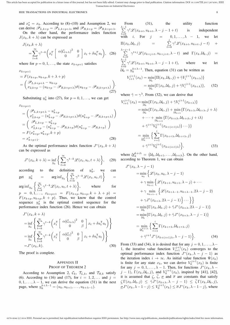
According to Assumption 2, Ck, TL,k, and TR,k satisfy(6). According to (16) and (17), for i = 1, 2, . . . and j =0, 1, . . . , λ − 1, we can derive the equation (31) in the nextpage, where uk+λ−1

k = (uk, uk+1, . . . , uk+λ−1).

From (31), the utility functionλ−1∑t=0

γtL (xk+t, uk+t, λ− j − 1 + t) is independent

with i. For j = 0, 1, . . . , λ − 1, we let

Π(xk,Uk, j) =j∑

t=0γtL (xk+t, uk+t, j − t) +

λ−j−1∑t=0

γt+jL (xk+j+t, uk+j+t, λ− t) and Γ(xk,Uk, j) =

λ−1∑t=0

γtL (xk+t, uk+t, λ− j − 1 + t), where we let

Uk = uk+λ−1k . Then, equation (31) can be written as

V j+1i+1 (xk) = min

Uk

{Π(xk,Uk, j) + γ̃V j+1i (xk+λ)}

= minUk

{Γ(xk,Uk, j) + γ̃V j+1i (xk+λ)}, (32)

where γ̃ = γλ. From (32), we can derive that

V j+1i+1 (xk) =min

Uk

{Γ(xk,Uk, j) + γ̃V j+1i (xk+λ)}

=minUk

{Γ(xk,Uk, j) + minUk+λ

{Γ(xk+λ,Uk+λ, j + λ)

+ · · ·+ minUk+iλ

{Γ(xk+iλ,Uk+iλ, j + iλ)

+ γ̃i+1V j+10 (xk+(i+1)λ)} · · · }}

= minUk+iλ

k

{ i∑τ=1

Γ(xk+τλ,Uk+τλ, j)

+ γ̃i+1V j+10 (xk+(i+1)λ)

}, (33)

where Uk+iλk =

(Uk,Uk+1, . . . ,Uk+iλ

). On the other hand,

according to Theorem 1, we can obtain

J∗(xk, λ− j − 1)

=minuk

{L (xk, uk, λ− j − 1)

+ γ minuk+1

{L (xk+1, uk+1, λ− j) + · · ·

+ γ minuk+λ−1

{L (xk+λ−1, uk+λ−1, 2λ− j − 2)

+ γJ∗(xk+λ, 2λ− j − 1)}· · ·

}}=min

Uk

{Γ(xk,Uk, j) + γ̃J∗(xk+λ, 2λ− j − 1)}

=minUk

{Γ(xk,Uk, j) + γ̃J∗(xk+λ, λ− j − 1)}

= minUk+iλ

k

{ i∑τ=1

Γ(xk+τλ,Uk+τλ, j)

+ γ̃i+1J∗(xk+(i+1)λ, λ− j − 1)}. (34)

From (33) and (34), it is desired that for any j = 0, 1, . . . , λ−1, the iterative value function V j+1

i+1 (xk) converges to theoptimal performance index function J∗(xk, λ − j − 1) asthe iteration index i → ∞. As initial value function Ψ(xk)is finite for any state xk, we can derive V j+1

0 (xk) is finitefor any j = 0, 1, . . . , λ − 1. Then, for functions J∗(xk, λ −j − 1), Γ(xk,Uk, j), and V j+1

0 (xk), inspired by [41], [42],it is assumed that ζ, ζ, σ and σ are constants that satisfyζ Γ(xk,Uk, j) ≤ γ̃J∗(xk+λ, λ − j − 1) ≤ ζ Γ(xk,Uk, j),σJ∗(xk, λ− 1− j) ≤ V j+1

0 (xk) ≤ σJ∗(xk, λ− 1− j), where




Vij+1(xk)

=minuk

{U (xk, uk, j) + γV j

i (xk+1)}

=minuk

{U (xk, uk, j) + γ min

uk+1

{U (xk+1, uk+1, j − 1) + · · ·+ γ min

uk+j

{U (xk+j , uk+j , 0) + γV 0

i (xk+j)}· · ·

}}=min

uk


uk+1

{U (xk+1, uk+1, j − 1) + · · ·+ γ min

uk+j

{U (xk+j , uk+j , 0) + γV λ

i−1(xk+j)}· · ·

}}=min

uk


uk+1

{U (xk+1, uk+1, j − 1) + · · ·+ γ min

uk+j

{U (xk+j , uk+j , 0)

+ γ minuk+j+1

{U (xk+j , uk+j , λ− 1) + · · ·+ min

uk+λ−1

{U (xk+λ−1, uk+λ−1, j + 1) + γV j+1

i−1 (xk+λ)}· · ·

}}· · ·

}}=min

uk

{L (xk, uk, λ− j − 1) + γ min

uk+1

{L (xk+1, uk+1, λ− j) + · · ·+ γ min

uk+j

{L (xk+j , uk+j , λ− 1)

+ γ minuk+j+1

{L (xk+j , uk+j , λ) + · · ·+ min

uk+λ−1

{L (xk+λ−1, uk+λ−1, 2λ− j − 2) + γV j+1

i−1 (xk+λ)}· · ·

}}· · ·

}}= min

uk+λ−1k

{ λ−1∑t=0

γtL (xk+t, uk+t, λ− j − 1 + t) + γλV j+1i−1 (xk+λ)

}. (31)

0 < ζ ≤ ζ < ∞ and 0 ≤ σ ≤ 1 ≤ σ < ∞. Let i = 1. Forany j = 0, 1, . . . , λ − 1, according to the idea in [41], [42],we can obtain

V j+11 (xk) =min

Uk

{Γ(xk,Uk, j) + γ̃V j+1

0 (xk+λ)}

≤minUk

{Γ(xk,Uk, j) + γ̃σJ∗(xk+λ, λ− j − 1)

}≤min

Uk

{(1 +

σ − 1

(1 + ζ̄)ζ̄)Γ(xk,Uk, j)

+(σ − σ − 1

(1 + ζ)

)γ̃J∗(xk+λ, λ− j − 1

)}=(1 +

σ − 1

(1 + ζ−1

)

)J∗(xk, λ− j − 1). (35)

According to mathematical induction, we can obtain(1+

σ − 1

(1 + ζ −1)i

)J∗(xk, λ− j − 1) ≤ V j+1

i (xk)

≤(1 +

σ − 1

(1 + ζ−1

)i

)J∗(xk, λ− j − 1). (36)

Letting i → ∞, we can obtain (20), which completes theproof.

REFERENCES

[1] C. S. Lai and M. D. McCulloch, “Sizing of stand-alone solar PV andstorage system with anaerobic digestion biogas power plants,” IEEETransactions on Industrial Electronics, article in press, 2016. DOI:10.1109/TIE.2016.2625781

[2] H. Liu, P. C. Loh, X. Wang, Y. Yang, W. Wang, and D. Xu, “Droopcontrol with improved disturbance adaption for a PV system with twopower conversion stages,” IEEE Transactions on Industrial Electronics,vol. 63, no. 10, pp. 6073–6085, Oct. 2016.

[3] E. Chatzinikolaou and D. J. Rogers, “Cell SoC balancing using a cascad-ed full-bridge multilevel converter in battery energy storage systems,”IEEE Transactions on Industrial Electronics, vol. 63, no. 9, pp. 5394–5402, Sep. 2016.

[4] Q. Shafiee, C. Stefanovic, T. Dragicevic, P. Popovski, J. C. Vasquez, andJ. M. Guerrero, “Robust networked control scheme for distributed sec-ondary control of islanded microgrids,” IEEE Transactions on IndustrialElectronics, vol. 61, no. 10, pp. 5363–5374, Oct. 2014.

[5] J. Appen, T. Stetz, M. Braun, and A. Schmiegel, “Local voltagecontrol strategies for PV storage systems in distribution grids,” IEEETransactions on Smart Grid, vol. 5, no. 2, pp. 1002–1009, Mar. 2014.

[6] S. Park, J. Lee, S. Bae, G. Hwang, and J. Choi, “Contribution basedenergy trading mechanism in micro-grids for future smart grid: A gametheoretic approach,” IEEE Transactions on Industrial Electronics, articlein press, 2016. DOI: 10.1109/TIE.2016.2532842

[7] Y. Lee, W. Hsiao, C. Huang, and S. T. Chou, “An integrated cloud-based smart home management system with community hierarchy,”IEEE Transactions on Consumer Electronics, vol. 62, no. 1, pp. 1–9,Jan. 2016.

[8] Q. Wei, D. Liu, Y. Liu, and R. Song, “Optimal constrained self-learningbattery sequential management in microgrids via adaptive dynamicprogramming,” IEEE/CAA Journal of Automatica Sinica, accept forpublication, 2016. DOI: 10.1109/JAS.2016.7510262

[9] F. L. Lewis, D. Vrabie, and K. G. Vamvoudakis, “Reinforcementlearning and feedback control: Using natural decision methods to designoptimal adaptive controllers,” IEEE Control Systems, vol. 32, no. 6, pp.76–105, Dec. 2012.

[10] Q. Yang, S. Jagannathan, and Y. Sun, “Robust integral of neural networkand error sign control of MIMO nonlinear systems,” IEEE Transactionson Neural Networks and Learning Systems, vol. 26, no. 12, pp. 3278–3286, Dec. 2015.

[11] Y. Jiang and Z. P. Jiang, “Robust adaptive dynamic programming andfeedback stabilization of nonlinear systems,” IEEE Transactions onNeural Networks and Learning Systems, vol. 25, no. 5, pp. 882–893,May 2014.

[12] Z. Ni, H. He, D. Zhao, X. Xu, and D. V. Prokhorov, “GrDHP: A generalutility function representation for dual heuristic dynamic programming,”IEEE Transactions on Neural Networks and Learning Systems, vol. 26,no. 3, pp. 614–627, Mar. 2015.

[13] Q. Wei, D. Liu, and H. Lin, “Value iteration adaptive dynamic pro-gramming for optimal control of discrete-time nonlinear systems,” IEEETransactions on Cybernetics, vol. 46, no. 3, pp. 840–853, Mar. 2016.

[14] Q. Wei, R. Song, and P. Yan, “Data-driven zero-sum neuro-optimalcontrol for a class of continuous-time unknown nonlinear systems withdisturbance using ADP,” IEEE Transactions on Neural Networks andLearning Systems, vol. 27, no. 2, pp. 444–458, Feb. 2016.

[15] Q. Wei, D. Liu, and X. Yang, “Infinite horizon self-learning optimalcontrol of nonaffine discrete-time nonlinear systems,” IEEE Transactionson Neural Networks and Learning Systems, vol. 26, no. 4, pp. 866–879,Apr. 2015.

[16] Q. Wei, F. Wang, D. Liu, and X. Yang, “Finite-approximation-errorbased discrete-time iterative adaptive dynamic programming,” IEEETransactions on Cybernetics, vol. 44, no. 12, pp. 2820–2833, Dec. 2014.

[17] Q. Wei and D. Liu, “Data-driven neuro-optimal temperature controlof water gas shift reaction using stable iterative adaptive dynamicprogramming,” IEEE Transactions on Industrial Electronics, vol. 61,no. 11, pp. 6399–6408, Nov. 2014.




[18] Q. Wei, F. L. Lewis, D. Liu, R. Song, and H. Lin, “Discrete-time localvalue Iteration adaptive dynamic programming: Convergence analysis,”IEEE Transactions on Systems, Man, and Cybernetics: Systems, articlein press, 2016. DOI: 10.1109/TSMC.2016.2623766

[19] R. Song, F. L. Lewis, Q. Wei, H. Zhang, Z. Jiang, and D. Levine,“Multiple actor-critic structures for continuous-time optimal controlusing input-output data,” IEEE Transactions on Neural Networks andLearning Systems, vol. 26, no. 4, pp. 851–865, Apr. 2015.

[20] R. Song, F. L. Lewis, Q. Wei, and H. Zhang, “Off-policy actor-criticstructure for optimal control of unknown systems with disturbances,”IEEE Transactions on Cybernetics, vol. 46, no. 5, pp. 1041–1050, Apr.2016.

[21] Q. Wei, D. Liu, G. Shi, and Y. Liu, “Optimal multi-battery coordinationcontrol for home energy management systems via distributed iterativeadaptive dynamic programming,” IEEE Transactions on Industrial Elec-tronics, vol. 42, no. 7, pp. 4203–4214, Jul. 2015.

[22] Q. Wei, D. Liu, F. L. Lewis, and Y. Liu, “Mixed iterative adaptivedynamic programming for optimal battery energy control in smartresidential microgrids,” IEEE Transactions on Industrial Electronics,accept, 2016. DOI: 10.1109/TIE.2017.2650872

[23] R. Song, W. Xiao, H. Zhang, and C. Sun, “Adaptive dynamic pro-gramming for a class of complex-valued nonlinear systems,” IEEETransactions on Neural Networks and Learning Systems, vol. 25, no.9, pp. 1733–1739, Sep. 2014.

[24] G. K. Venayagamoorthy, R. K. Sharma, P. K. Gautam, and A. Ahmadi,“Dynamic energy management system for a smart microgrid,” IEEETransactions on Neural Networks and Learning Systems, article in press,2016. DOI: 10.1109/TNNLS.2016.2514358

[25] T. Huang and D. Liu, “A self-learning scheme for residential energysystem control and management,” Neural Computing and Applications,vol. 22, no. 2, pp. 259–269, Feb. 2013.

[26] J. Si and Y.-T. Wang, “On-line learning control by association andreinforcement,” IEEE Transactions on Neural Networks, vol. 12, no.2, pp. 264–276, Mar. 2001.

[27] M. Boaro, D. Fuselli, F. D. Angelis, D. Liu, Q. Wei, and F. Piaz-za, “Adaptive dynamic programming algorithm for renewable energyscheduling and battery management,” Cognitive Computation, vol. 5,no. 2, pp. 264–277, Jun. 2013.

[28] D. Fuselli, F. D. Angelis, M. Boaro, D. Liu, Q. Wei, S. Squartini, andF. Piazza, “Action dependent heuristic dynamic programming for homeenergy resource scheduling,” International Journal of Electrical Powerand Energy Systems, vol. 48, pp. 148–160, Jun. 2013.

[29] L. Dong, Y. Tang, H. He, and C. Sun, “An event-triggered approachfor load frequency control with supplementary ADP,” IEEE Trans-actions on Power Systems, article in press, 2016. DOI: 10.1109/TP-WRS.2016.2537984

[30] Q. Wei, D. Liu, and G. Shi, “A novel dual iterative Q-learning methodfor optimal battery management in smart residential environments,”IEEE Transactions on Industrial Electronics, vol. 62, no. 4, pp. 2509–2518, Apr. 2015.

[31] National renewable energy laboratory (NREL) of U.S. Department ofEnergy, Office of Energy Efficiency and Renewable Energy, operatedby the Alliance for Sustainable Energy, LLC. [Online]. Available:http://www.nrel.gov/rredc/

[32] T. Markvart, Solar electricity (2nd Edition). New York: Wiley, 2000.[33] T. Y. Lee, “Operating schedule of battery energy storage system in a

time-of-use rate industrial user with wind turbine generators: A multi-pass iteration particle swarm optimization approach,” IEEE Transactionson Energy Conversion, vol. 22, no. 3, pp. 774–782, Mar. 2007.

[34] T. Yau, L. N. Walker, H. L. Graham, and R. Raithel, “Effects of batterystorage devices on power system dispatch,” IEEE Transactions on PowerApparatus and Systems, vol. PAS-100, no. 1, pp. 375–383, Jan. 1981.

[35] Data of electricity rate from ComEd Company, USA. [Online].https://rrtp.comed.com/live-prices/?.

[36] NAHB Research Center, Inc., “Review of residential electrical energyuse data,” 400 Prince George’s Boulevard Upper Marlboro, MD, USA,July 16, 2001. [Online]. http://www.toolbase.org/PDF/CaseStudies /Res-Electrical-EnergyUseData.pdf

[37] T. Wang, H. Kamath, and S. Willard, “Control and otimization of grid-tied photovoltaic storage systems using model predictive control,” IEEETransactions on Smart Grid, vol. 5, no. 2, pp. 1010–1017, Mar. 2014.

[38] E. F. Camacho and C. Bordons, Model Predictive Control. Berlin,Germany: Springer, 1999.

[39] J. T. Betts, Practical Methods for Optimal Control and EstimationUsing Nonlinear Programming. Philadelphia: Society for Industrial andApplied Mathematics, 2010.

[40] ComEd, USA, http://www.thewattspot.com. Accessed 16 May 2010.

[41] B. Lincoln and A. Rantzer, “Relaxing dynamic programming,” IEEETransactions on Automatic Control, vol. 51, no. 8, pp. 1249–1260, Aug.2006.

[42] A. Rantzer, “Relaxed dynamic programming in switching systems,” IETControl Theory and Applications vol. 153, no. 5, pp. 567–574, Sep.2006.

Qinglai Wei (M’11) received Ph.D. degree in con-trol theory and control engineering, from the North-eastern University, Shenyang, China, in 2009. From2009–2011, he was a postdoctoral fellow with TheState Key Laboratory of Management and Controlfor Complex Systems, Institute of Automation, Chi-nese Academy of Sciences, Beijing, China. He iscurrently a Professor of the institute. He is also aProfessor of the University of Chinese Academy ofSciences. He has authored two books, and publishedover 60 international journal papers. His research

interests include adaptive dynamic programming, neural-networks-based con-trol, optimal control, nonlinear systems and their industrial applications.

Dr. Wei is an Associate Editor of IEEE Transaction on Systems Man,and Cybernetics: Systems since 2016, Information Sciences since 2016,Neurocomputing since 2016, Optimal Control Applications and Methods since2016, Acta Automatica Sinica since 2015, and has been holding the sameposition for IEEE Transactions on Neural Networks and Learning Systemsduring 2014–2015. He is the Secretary of IEEE Computational IntelligenceSociety (CIS) Beijing Chapter since 2015.

Guang Shi received the B.S. degree in automationfrom Zhejiang University, Hangzhou, China, in July,2012. Currently, he is working towards the Ph.D.degree at The State Key Laboratory of Managementand Control for Complex Systems, Institute of Au-tomation, Chinese Academy of Sciences, Beijing,China. His research interests include neural network-s, adaptive dynamic programming, optimal controland energy management in smart grids.

Ruizhuo Song (M’11) received the Ph.D. degree incontrol theory and control engineering from North-eastern University, Shenyang, China, in 2012. She iscurrently an associate professor with the School ofAutomation and Electrical Engineering, Universityof Science and Technology Beijing. Her researchinterests include optimal control, neural-networks-based control, nonlinear control, wireless sensornetworks, adaptive dynamic programming and theirindustrial application.

Yu Liu received the B.S. degree in automation,the M.S. degree in Pattern Recognition and Intelli-gent Systems, from Beijing Institute of Technology,Beijing, China, in 2001 and 2004 respectively, andthe Ph.D. degree in Pattern Recognition and Intel-ligent Systems, from Institute of Automation, Chi-nese Academy of Sciences, Beijing, China, in 2010.His research interests include artificial intelligence,streaming data analysis, and energy management insmart grids.

IEEE TRANSACTIONS ON INDUSTRIAL ELECTRONICS 1 Adaptive ...

Documents

Transcript of IEEE TRANSACTIONS ON INDUSTRIAL ELECTRONICS 1 Adaptive ...