IEEE TRANSACTIONS ON CONTROL SYSTEMS TECHNOLOGY 1 Dynamic ...frborrel/pdfpub/Alex2016.pdf ·...

This article has been accepted for inclusion in a future issue of this journal. Content is final as presented, with the exception of pagination.

IEEE TRANSACTIONS ON CONTROL SYSTEMS TECHNOLOGY 1

Dynamic Positioning With Model Predictive ControlAleksander Veksler, Member, IEEE, Tor Arne Johansen, Senior Member, IEEE,

Francesco Borrelli, Senior Member, IEEE, and Bjørnar Realfsen

Abstract— Marine vessels with dynamic positioning (DP)capability are typically equipped with sufficient number ofthrusters to make them overactuated and with satellite navigationand other sensors to determine their position, heading, andvelocity. An automatic control system is tasked with coordinatingthe thrusters to move the vessel in any desired direction and tocounteract the environmental forces. The design of this controlsystem is usually separated into several levels. First, a DP controlalgorithm calculates the total force and moment of force that thethruster system should produce. Then, a thrust allocation (TA)algorithm coordinates the thrusters so that the resultant forcethey produce matches the request from the DP control algorithm.Unless significant heuristic modifications are made, theDP control algorithm has limited information about the thrustereffects such as saturations and limited rate of rotation of variable-direction thrusters, as well as systemic effects such as singularthruster configurations. The control output produced with thiscontrol architecture is therefore not always optimal, and mayresult in a position loss that would not have occurred with a moresophisticated control algorithm. Recent advances in computerhardware and algorithms make it possible to consider a model-predictive control (MPC) algorithm that combines positioningcontrol and TA into a single algorithm, which should theoreticallyyield a near-optimal controller output. This paper explores theadvantages and disadvantages of using MPC compared with thetraditional algorithms.

Index Terms— Marine vehicles, motion control, optimalcontrol, path planning, position control, predictive control.

I. INTRODUCTION

AMARINE vessel is said to have dynamic position-ing (DP) capability if it is able to maintain a prede-

termined position and heading automatically exclusively bymeans of thruster force [1]. DP is therefore an alternative and,sometimes, a supplement to the more traditional solution of

Manuscript received May 25, 2015; accepted August 29, 2015. Manuscriptreceived in final form October 25, 2015. This work was supported bythe Research Council of Norway, Kongsberg Maritime, and Det NorskeVeritas, through the Knowledge Building Project Design to verification underProject 210670 and Project 192427, and through the Centres of ExcellenceFunding Scheme under Project 223254–Center for Autonomous MarineOperations and Systems. Recommended by Associate Editor E. Kerrigan.(Corresponding author: Aleksander Veksler.)

A. Veksler is with Step Solutions, Oslo 0473, Norway (e-mail: [email protected]).

T. A. Johansen is with the Center for Autonomous Marine Operationsand Systems, Department of Engineering Cybernetics, Norwegian Universityof Science and Technology, Trondheim 7491, Norway (e-mail: [email protected]).

F. Borrelli is with the Model Predictive Control Laboratory, Universityof California at Berkeley, Berkeley, CA 94720 USA (e-mail: [email protected]).

B. Realfsen is with Kongsberg Maritime, Kongsberg 3616, Norway (e-mail:[email protected]).

Color versions of one or more of the figures in this paper are availableonline at http://ieeexplore.ieee.org.

Digital Object Identifier 10.1109/TCST.2015.2497280

anchoring a ship to the seabed. The advantages of positioninga ship with the thrusters instead of anchoring it include thefollowing.

1) Immediate position setpoint acquiring and reacquiring.A position setpoint change can usually be done with acommand from an operator station, whereas a significantposition change for an anchored vessel would require aphysical repositioning of the anchors.

2) Anchors can operate on depths of only up toabout 500 m. No such limitations are present with DP.

3) No risk of damage to seabed infrastructure and risers,which allows safe and flexible operation in crowdedoffshore production fields.

4) Accurate control of position and heading.The main disadvantages are that a ship has to be specificallyequipped to operate in DP, and that dynamically positionedships consume more power to stay in position, even thoughanchored vessels also have to expend energy to continuouslyadjust the tension in the mooring lines.

DP is usually installed on offshore service vessels, ondrill rigs, and now increasingly on production platforms thatare intended to operate on locations that are so deep thatpermanent attachment to the sea floor with, e.g., mooringlines is impractical. Several thousand ships worldwide haveDP installed.

Depending on its function, a DP vessel that fails to keepits position may risk colliding with other vessels, endangerdivers, interrupt operations, and/or cause damage to equip-ment such as risers. Vessels that are designed to performreliably typically have a high degree of redundancy in allcritical systems, including power generation, thrusters, and thecomputer system. Classification societies such as Det NorskeVeritas German Lloyds and International Maritime Organiza-tion (IMO) issue standards that include safety regulations forthe DP systems. For example, to be classified as IMO Class2, the DP system has to be designed with redundancies in thepower distribution system, power generation, thruster system,and many others; in particular, the thruster system must con-tinue to be fully capable after a failure of any single thruster.

The algorithm that coordinates the thrusters to keep asetpoint position and orientation is called the DP algorithm.A commonality for most control algorithms that are avail-able in the literature is that they separate the control taskinto two parts. First, a high-level motion control algorithmconsiders the current position and heading of the ship, anddetermines the total force and moment of force (togethercalled generalized force, further explained in Appendix B)that needs to be applied on the ship. Somewhat ambiguously,this algorithm is usually called the DP control algorithm.

1063-6536 © 2016 IEEE. Personal use is permitted, but republication/redistribution requires IEEE permission.See http://www.ieee.org/publications_standards/publications/rights/index.html for more information.


2 IEEE TRANSACTIONS ON CONTROL SYSTEMS TECHNOLOGY

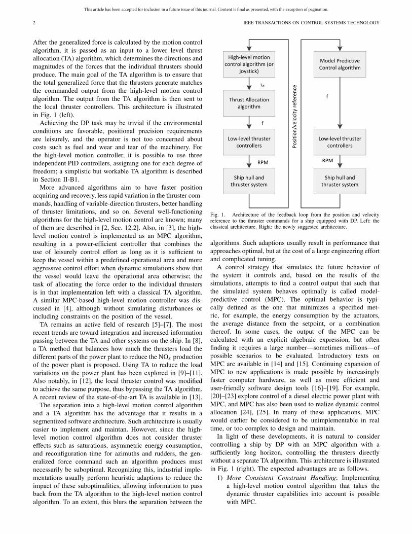
After the generalized force is calculated by the motion controlalgorithm, it is passed as an input to a lower level thrustallocation (TA) algorithm, which determines the directions andmagnitudes of the forces that the individual thrusters shouldproduce. The main goal of the TA algorithm is to ensure thatthe total generalized force that the thrusters generate matchesthe commanded output from the high-level motion controlalgorithm. The output from the TA algorithm is then sent tothe local thruster controllers. This architecture is illustratedin Fig. 1 (left).

Achieving the DP task may be trivial if the environmentalconditions are favorable, positional precision requirementsare leisurely, and the operator is not too concerned aboutcosts such as fuel and wear and tear of the machinery. Forthe high-level motion controller, it is possible to use threeindependent PID controllers, assigning one for each degree offreedom; a simplistic but workable TA algorithm is describedin Section II-B1.

More advanced algorithms aim to have faster positionacquiring and recovery, less rapid variation in the thruster com-mands, handling of variable-direction thrusters, better handlingof thruster limitations, and so on. Several well-functioningalgorithms for the high-level motion control are known; manyof them are described in [2, Sec. 12.2]. Also, in [3], the high-level motion control is implemented as an MPC algorithm,resulting in a power-efficient controller that combines theuse of leisurely control effort as long as it is sufficient tokeep the vessel within a predefined operational area and moreaggressive control effort when dynamic simulations show thatthe vessel would leave the operational area otherwise; thetask of allocating the force order to the individual thrustersis in that implementation left with a classical TA algorithm.A similar MPC-based high-level motion controller was dis-cussed in [4], although without simulating disturbances orincluding constraints on the position of the vessel.

TA remains an active field of research [5]–[7]. The mostrecent trends are toward integration and increased informationpassing between the TA and other systems on the ship. In [8],a TA method that balances how much the thrusters load thedifferent parts of the power plant to reduce the NOx productionof the power plant is proposed. Using TA to reduce the loadvariations on the power plant has been explored in [9]–[11].Also notably, in [12], the local thruster control was modifiedto achieve the same purpose, thus bypassing the TA algorithm.A recent review of the state-of-the-art TA is available in [13].

The separation into a high-level motion control algorithmand a TA algorithm has the advantage that it results in asegmentized software architecture. Such architecture is usuallyeasier to implement and maintan. However, since the high-level motion control algorithm does not consider thrustereffects such as saturations, asymmetric energy consumption,and reconfiguration time for azimuths and rudders, the gen-eralized force command such an algorithm produces mustnecessarily be suboptimal. Recognizing this, industrial imple-mentations usually perform heuristic adaptions to reduce theimpact of these suboptimalities, allowing information to passback from the TA algorithm to the high-level motion controlalgorithm. To an extent, this blurs the separation between the

Fig. 1. Architecture of the feedback loop from the position and velocityreference to the thruster commands for a ship equipped with DP. Left: theclassical architecture. Right: the newly suggested architecture.

algorithms. Such adaptions usually result in performance thatapproaches optimal, but at the cost of a large engineering effortand complicated tuning.

A control strategy that simulates the future behavior ofthe system it controls and, based on the results of thesimulations, attempts to find a control output that such thatthe simulated system behaves optimally is called model-predictive control (MPC). The optimal behavior is typi-cally defined as the one that minimizes a specified met-ric, for example, the energy consumption by the actuators,the average distance from the setpoint, or a combinationthereof. In some cases, the output of the MPC can becalculated with an explicit algebraic expression, but oftenfinding it requires a large number—sometimes millions—ofpossible scenarios to be evaluated. Introductory texts onMPC are available in [14] and [15]. Continuing expansion ofMPC to new applications is made possible by increasinglyfaster computer hardware, as well as more efficient anduser-friendly software design tools [16]–[19]. For example,[20]–[23] explore control of a diesel electric power plant withMPC, and MPC has also been used to realize dynamic controlallocation [24], [25]. In many of these applications, MPCwould earlier be considered to be unimplementable in realtime, or too complex to design and maintain.

In light of these developments, it is natural to considercontrolling a ship by DP with an MPC algorithm with asufficiently long horizon, controlling the thrusters directlywithout a separate TA algorithm. This architecture is illustratedin Fig. 1 (right). The expected advantages are as follows.

1) More Consistent Constraint Handling: Implementinga high-level motion control algorithm that takes thedynamic thruster capabilities into account is possiblewith MPC.


VEKSLER et al.: DP WITH MPC 3

2) Planning Ahead: Even with a reasonably short horizon,an MPC can plan ahead maneuvers instead of goingtoward the goal in the most direct manner possible.Such maneuvers include moving the vessel towardthe setpoint along a trajectory that is optimal andcoordinated with respect to the saturation limits of thethrusters, as well as their direction and rate of turnwhere this is applicable. If the MPC is implementedwith a sufficiently long horizon, it may be able to escapefrom local minima. A typical example is when a rotablebidirectional thruster is working in a direction in whichits propeller is suboptimal, and should be turned around.

3) Simpler Design and Tuning: The MPC intrinsicallyresolves a number of idiosyncrasies that requirecomplex adaptions with the traditional architectures,and the engineering effort that is required to design anMPC controller is therefore expected to be smaller.

The first and second advantages are mainly in reduced powerconsumption and reduced position deviation in situations withlimited thrust and power. For the third one, the advantage is inreduced development cost and faster time to market; the timespent configuring the DP system on-site may also be reduced,although it is usually possible to do most of the configurationwork off-site with hardware-in-the-loop simulation [26].

The goal of this paper is to explore the advantages andchallenges of using MPC as a dynamic positioning controller,and to determine if this technology is viable for real-lifeuse. In this work we chose to simplify the formulation byavoiding any explicit stability-enforcing terms or constraints.The main reason for this is that a sufficiently large predictionhorizon is sufficient to guarantee stability [27]. Moreover, thesystem is not unstable, and simulations show no problems withstability. If it is necessary to reduce the prediction horizonto simplify computations in an industrial implementation,stability and performance might be influenced. It is well knownhow to redesign MPC with stability-enhancing cost terms andconstraints [15].

Potential practitioners should be aware of the limited scopeof this paper. A practical DP control system would have tohandle many additional complications that are not consideredin this implementation. Such complications include model-plant mismatches in all parts of the model, imperfect positionreference, and wave filters. Practical DP codes tend for thesereasons to become very large and remain proprietary.

The structure of this paper is as following. The mathe-matical model that is used for forecasting is described inSection II, and the MPC problem is formulated and discussedin Section III. Its implementation as a computer program isdiscussed in Section IV. The proposed MPC controller wastested in simulation, and the results from four simulationscenarios are presented in Section V. A glossary of some ofthe more important terms can be found in Appendix B.

II. BRIEF INTRODUCTION TO MODELING

OF MARINE VESSELS

This section provides a basic explanation of the model thatis used to implement the MPC in this paper.

TABLE I

ABBREVIATIONS THAT ARE USED TO DESCRIBE THE POSITIONAND VELOCITY OF THE VESSEL, AS PER CONVENTION

FROM [2, p. 19] AND [28]

Fig. 2. Coordinate systems. (a) Position of the vessel is defined in the NEDcoordinate system. (b) Velocity is defined in the body coordinate system.

A. Geometry and Kinematics

The investigation that is presented here deals with a shipthat moves on the ocean surface at relatively low velocities.The roll and pitch motions of the vessel are neither monitorednor compensated. The mathematical model that is used todescribe the system can therefore be kept reasonably simpleby limiting it to the planar position and orientation of thevessel. A coordinate system is selected with the origin at theDP setpoint, the x-axis pointing to north, the y-axis pointingto east, and the (unused) z-axis pointing downward per theright-hand rule. The orientation of the ship in the xy planeis defined as clockwise rotation with the orientation with thebow pointing to the north as the zero reference.

The velocity of the vessel is usually described in its ownframe of reference called the body coordinate system. Thevelocity vector ν consists of components u, v, r , that describethe velocity in the directions forwards toward the bow,sideways towards the starboard, and clockwise yaw rotation.The abbreviations that are used to describe the position and



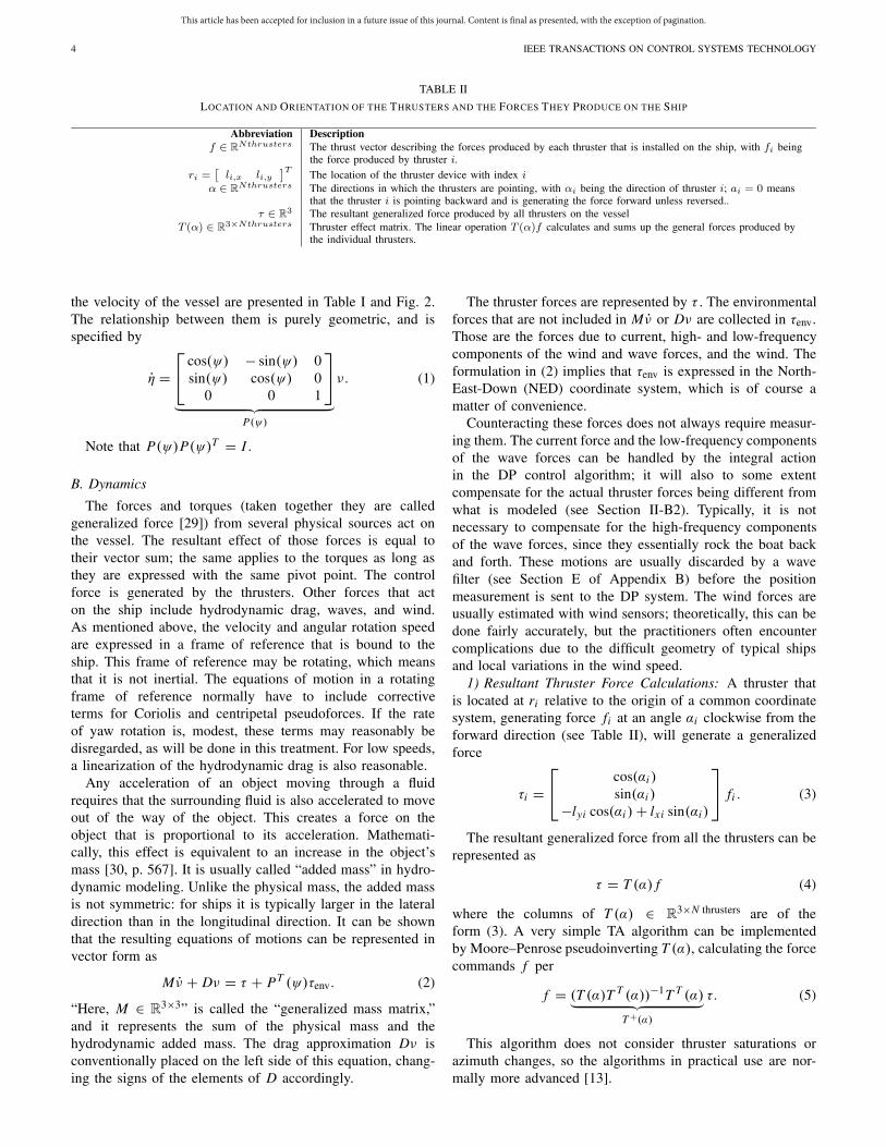
TABLE II

LOCATION AND ORIENTATION OF THE THRUSTERS AND THE FORCES THEY PRODUCE ON THE SHIP

the velocity of the vessel are presented in Table I and Fig. 2.The relationship between them is purely geometric, and isspecified by

η =⎡⎣

cos(ψ) − sin(ψ) 0sin(ψ) cos(ψ) 0

0 0 1

⎤⎦

︸︷︷︸P(ψ)

ν. (1)

Note that P(ψ)P(ψ)T = I .

B. Dynamics

The forces and torques (taken together they are calledgeneralized force [29]) from several physical sources act onthe vessel. The resultant effect of those forces is equal totheir vector sum; the same applies to the torques as long asthey are expressed with the same pivot point. The controlforce is generated by the thrusters. Other forces that acton the ship include hydrodynamic drag, waves, and wind.As mentioned above, the velocity and angular rotation speedare expressed in a frame of reference that is bound to theship. This frame of reference may be rotating, which meansthat it is not inertial. The equations of motion in a rotatingframe of reference normally have to include correctiveterms for Coriolis and centripetal pseudoforces. If the rateof yaw rotation is, modest, these terms may reasonably bedisregarded, as will be done in this treatment. For low speeds,a linearization of the hydrodynamic drag is also reasonable.

Any acceleration of an object moving through a fluidrequires that the surrounding fluid is also accelerated to moveout of the way of the object. This creates a force on theobject that is proportional to its acceleration. Mathemati-cally, this effect is equivalent to an increase in the object’smass [30, p. 567]. It is usually called “added mass” in hydro-dynamic modeling. Unlike the physical mass, the added massis not symmetric: for ships it is typically larger in the lateraldirection than in the longitudinal direction. It can be shownthat the resulting equations of motions can be represented invector form as

M ν + Dν = τ + PT (ψ)τenv. (2)

“Here, M ∈ R3×3” is called the “generalized mass matrix,”

and it represents the sum of the physical mass and thehydrodynamic added mass. The drag approximation Dν isconventionally placed on the left side of this equation, chang-ing the signs of the elements of D accordingly.

The thruster forces are represented by τ . The environmentalforces that are not included in M ν or Dν are collected in τenv.Those are the forces due to current, high- and low-frequencycomponents of the wind and wave forces, and the wind. Theformulation in (2) implies that τenv is expressed in the North-East-Down (NED) coordinate system, which is of course amatter of convenience.

Counteracting these forces does not always require measur-ing them. The current force and the low-frequency componentsof the wave forces can be handled by the integral actionin the DP control algorithm; it will also to some extentcompensate for the actual thruster forces being different fromwhat is modeled (see Section II-B2). Typically, it is notnecessary to compensate for the high-frequency componentsof the wave forces, since they essentially rock the boat backand forth. These motions are usually discarded by a wavefilter (see Section E of Appendix B) before the positionmeasurement is sent to the DP system. The wind forces areusually estimated with wind sensors; theoretically, this can bedone fairly accurately, but the practitioners often encountercomplications due to the difficult geometry of typical shipsand local variations in the wind speed.

1) Resultant Thruster Force Calculations: A thruster thatis located at ri relative to the origin of a common coordinatesystem, generating force fi at an angle αi clockwise from theforward direction (see Table II), will generate a generalizedforce

τi =⎡⎣

cos(αi )sin(αi )

−lyi cos(αi )+ lxi sin(αi )

⎤⎦ fi . (3)

The resultant generalized force from all the thrusters can berepresented as

τ = T (α) f (4)

where the columns of T (α) ∈ R3×N thrusters are of the

form (3). A very simple TA algorithm can be implementedby Moore–Penrose pseudoinverting T (α), calculating the forcecommands f per

f = (T (α)T T (α))−1T T (α)︸︷︷︸T+(α)

τ. (5)

This algorithm does not consider thruster saturations orazimuth changes, so the algorithms in practical use are nor-mally more advanced [13].



2) Relationship Between Generated Force, RPM, and PowerConsumption of the Thrusters: Dimensional analysis of apropeller in free water (i.e., far from a ship hull or otherobstructions and disturbances) combined with a few otherhydrodynamical assumptions leads to a model where, for apropeller that is stationary in water, both the trust and thetorque it produces are proportional to the square of its speedof rotation [31, p. 145].

The power that is required to keep a propeller at a constantspeed of rotation is the resistance torque times the speed ofrotation. It is therefore reasonable to assume that the powerthat is required to drive a propeller is approximately propor-tional to the power of 3/2, that is | fi |3/2. This approximationis used in many studies, including [10], [11], and [13]. Thiswork uses a penalty on the square of the force ( f 2

i ). Thisapproximately minimizes the power consumption and allowsfaster optimization problem solving. A penalty function likethis is used in, e.g., [6] and [7].

In this paper, the actual force that is produced by thethrusters is assumed to be the controlled variable. This assump-tion implies that the local thruster controllers can accept aforce setpoint [32].

C. Summary of the Model

The motion of a vessel in DP can thus be approximatedwith (1), (2), and (4). Restating them for the sake of clarity

η = P(ψ)ν (6)

M ν + Dν = τ + PT (ψ)τenv (7)

τ = T (α) f. (8)

III. MPC FORMULATION

The following continuous-time numerical optimization for-mulation summarizes the discussion in the previous section,and is proposed as a basis for the MPC of the dynamicalsystem:

J ∗ = minf +, f −,α

ˆ Te

0

{‖ f +‖2Q f+ + ‖ f −‖2Q f− + ‖α‖2Qα

+

+‖ν‖2Qν+ ‖η‖2Qη

+ ‖ˆ Te

0ηdt‖2Q´ η

}dt

+ similar terminal costs (9)

s.t. T (α) f + − T (α) f − = τ (10)

0 ≤ [ f +, f − ]T ≤ [ f , f ]T (11)

|α| ≤ ˙α (12)

M ν + Dν = τ − P(ψ)T τenv (13)

P(ψ)ν = η (14)

Initial conditions on η, ν, α (15)

τ (Te) = P(ψ)T τenv(Te). (16)

Implementation of this problem as a computer algorithm isexplained in Section IV. The thruster system constraint (10)is based on (8), but it is separated into a positive and anegative term to accommodate such thrusters. Such thrustersare designed for maximal efficiency in one direction, and areless efficient when running in reverse. The cost associated

with running them in reverse is for this reason higher, andusually the maximal attainable thrust is lower.

Similarly, constraint (11) limits the force produced by theindividual thrusters. Since not all thrusters can produce force innegative direction and some thrusters can produce more forcein positive direction than in negative, the values of f and fhave to be set separately.

The rate of change of the vector of azimuth angles forthe variable-angle thrusters α is limited in (12) because somethrusters such as azimuth thrusters and rudders cannot changetheir direction very quickly. The maximum rate of rotationvaries, but is typically on the scale of 30 s for a 360◦ turn.

With traditional TA algorithms, a slack term is often nec-essary in (10) to make sure that the allocation problem isfeasible even if a thrust command cannot be achieved. Such aterm is not necessary in this implementation, since τ representsthe actual generalized force on the vessel and not a setpointcommand as with the traditional thrust algorithms.

Constraints (13) and (14) are the dynamic and kinematicconstraints of the ship, and are a vector form formulation ofthe Newtonian laws of motion for the system as discussedin Section II. Environmental generalized force τenv representsthe resultant of the various environmental forces, such as wind,currents, waves, moorings, anchors, risers, cables (cable lay),pipes (pipe lay), hoses (offloading), and sea ice. Typically, thehigh-frequency component of the wave forces is filtered out ofthe model. The value of τenv at the initial time can be estimatedwith a combination of direct measurement with, e.g., wind sen-sors and model-based observers; the latter is mathematicallyequivalent to the integral action in a traditional PID controller.The future values of τenv can of course not be known, whichis one of the factors that limit the forecasting power of themodel. This will be further discussed in Section III-B.

The terminal costs represent how good the system state isat the end of the horizon. They can also be seen as a represen-tation of the costs that will be incurred after the optimizationhorizon. The only terminal costs that were found to benecessary in the tested models are the cost associated with thegeneralized position η and the cost associated with its integral.

Without the terminal constraint (16), the optimizer willturn off the thrusters at the end of the optimization horizon inthe open-loop simulation. In this way, it will capitalize on thefact that the resulting driftoff lags after the thrusters turn off;this driftoff cost will thus fall after the end of the predictionhorizon Te and thus outside (9). The open-loop trajectory willthus be suboptimal at the end of the horizon. The impact of thissuboptimality on the closed loop may be reduced by extendingthe length of the horizon, which of course would increasecomputational complexity.

The DP setpoint is set to the origin of the NED coordinatesystem without loss of generality.

A. Turning the Thrusters Around

A complication with the standard control architecture forDP is that the TA problem is often nonconvex. In practice,this means that a thruster may end up stuck either in anorientation where it has to produce thrust in a directionopposite to its optimal direction ( f − > 0), or, in case of



unidirectional thrusters, in an orientation where it cannotproduce any thrust that can be useful. A standard solutionto this is having an exogenous algorithm to evaluate thesituation, and turn the thrusters around if this is consid-ered beneficial (temporarily commandeering the orientationof the thruster in question from the TA algorithm). Othersources of nonconvexity are forbidden sectors and the use ofrudders [7], [13].

An MPC formulation with a horizon that is as long as theturnaround time for the thrusters could automatically considerif the thrusters should be turned or not. Care should be takenthat the numerical solver can either reliably find nonlocalminima, or, as in case with the test implementation inSection IV, that it is provided with an approximate directionfor where to look by means of an appropriate warm-starttrajectory.

The transition of the thrusters incurs a short-term cost, andunless the horizon is significantly longer than the turnaroundtime, the majority of the benefit of turning the thrusters isseen in the (reduction of the) terminal costs. Care shouldtherefore be taken during tuning to ensure that the terminalcosts correctly reflect the long-term advantage of having athruster point in the right direction.

B. Modeling Simplifications and Predictability

The MPC solver simulates the expected behavior of thevessel and calculates the thruster commands that result in abehavior of the ship that is optimal based on the specifiedcriteria. In general, the quality of MPC increases with thelength of the prediction horizon. However, the stochasticnature of the marine environment limits the predictive powerof any possible mathematical model. The predictive power ofthe mathematical model that is developed for this treatmentis certainly not improved by the approximations that weremade in Section II, but in practice the uncertainty about theparameters and the environment are likely to be more limitingthan the limitations of the model.

Constraint (13) requires an estimate of the environmentalforces τenv until the end of the simulation horizon Te (morespecifically, the part of the environmental forces that cannotbe predicted and filtered by the wave filter). It is technicallyconceivable, but not practical, to use the information fromnearby vessels or a fleet of unmanned aerial vehicles tomap the wind field and thus predict most of the variationsin the environmental forces some time ahead. Normally, theenvironmental forces do not change a lot during the timeused as the prediction horizon, so an approximation can bemade that the environmental force is constant and equal toits value at the beginning of the horizon. The latter can becalculated using an observer based on (2). The quality of anysuch estimate naturally degrades with increased length of Te.It is therefore unreasonable to expect that the forecasting madeby the MPC is a close approximation of the actual behaviorof the ship.

For these reasons, extending the prediction horizon Te

beyond a few seconds may not necessarily be better than otherheuristic adaptions.

IV. IMPLEMENTATION

In this section, the implementation of the continuous-timeMPC formulation (9)–(16) as a computer program will bediscussed.

The MPC problem formulation includes the azimuthrate constraint (12) and the the dynamic modelconstraints (13)–(14). If the state variables α, ν, and ηand the control outputs f +, f −, and α satisfy thoseconstraints, then they represent a possible trajectory of thesystem—in this case, a possible scenario for the movementof the vessel. Constraint (15) ensures that this trajectory isin fact a possible future trajectory of the vessel by matchingthe initial values of α, ν, and η to the current state of thephysical system.

Every future trajectory is associated with a cost J ∗,expressed by (9). There are costs associated with the use ofthruster force, with rotating the thrusters, and with positionand velocity deviations from the setpoint. A global solutionto this problem is a possible trajectory for the states andcontrol outputs that minimizes (9). Because of computationallimitations, this cost is evaluated only for a limited time,until Te.

The continuous-time formulation has to be discretized tobe solved on a digital computer. In a discrete-time represen-tation, the continuous-time trajectories of variables such asthe position of the ship and thruster forces are representedby a (finite) number of discrete samples; the continuous-timeconstraints should then be replaced with a finite number ofequality constraints between the samples. For example, witha prediction horizon of 45 s and discretization interval of0.5 s, there will be 90 discrete variables representing each(scalar) continuous variable. By doing this for each state andinput, it is possible to represent (9)–(16) as a—typically verylarge—numerical optimization problem; several algorithmsare available to solve such problems, both open source andcommercial.

Software packages that are capable of handling discrete-or continuous-time MPC formulations also exist. Typically,they will also automatically hand off the resulting discrete-time numerical optimization problem to a solver. The packagethat was selected for this project is called BLOM, which standsfor Berkeley Library for Optimization Modeling. It is designedto assist in rapid implementation of MPC by providing agraphical interface to allow users to create optimization prob-lems using Simulink. Using such a package allows significanttime savings compared with transforming the model into anumerical optimization problem, and graphical design usuallymeans faster and less error-prone implementation.

BLOM has a capability to handle discretization automati-cally, but in this implementation, the model was discretizedby hand with the forward Euler discretization scheme.

V. SIMULATION RESULTS

The proposed TA algorithm was tested in simulation, on amodel of SV Northern Clipper, featured in [33]. It is 76.20-mlong, with a mass of 4.591 · 106 kg. It has four thrusters,with two tunnel thrusters near the bow and two azimuth



TABLE III

SIMULATION SCENARIOS

TABLE IV

RELEVANT Bis NORMALIZATION CONSTANTS [2, TABLE 7.2]

thrusters at the stern. This configuration is illustrated in Fig. 3.The maximal force for each thruster was set to (1/60)of the ship’s dry weight. The turnaround time for thethrusters was set to relatively slow 60 s. All the thrusters arebidirectional; the tunnel thrusters in the bow are symmetric,while the azimuth thrusters use twice as much power toproduce force in reverse compared with their normal direc-tion. It was implemented in discrete-time in BLOM, using aforward Euler discretization with a 0.5-s discretization interval.Four simulations are reported. The difference between them isthat they have different starting conditions and different predic-tion horizons. Two of the scenarios have also increased relativeheading priority, to better reflect how they will typically beused. The differences between the scenarios are summarizedin Table III.

The environmental forces were set to be a constant windin the direction toward north. All numerical values weretransferred to per unit in the bis system per Table IV. Theperformance of the algorithm is compared with a baselinealgorithm with a standard architecture with a separate DPcontrol algorithm and a TA algorithm; it is based on elementsfrom several available publications on the topic, and it isdescribed in detail in Appendix A.

A. First Scenario

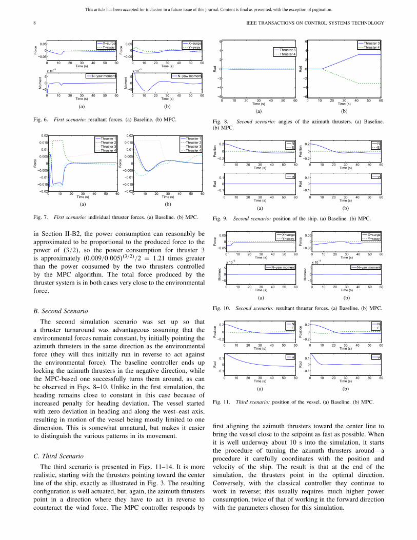
The first simulation is a deliberate worst case scenariofor the classical controller. Both azimuth thrusters initiallypoint toward the starboard, resulting in a singular thrusterconfiguration. At the start, there is no way for the thrustersystem to create force in the longitudinal direction where itis needed. The results are shown in Figs. 4–7. The classicalmotion control immediately drives the thrusters to saturation,forcing them to act against one another without producingmuch force in total. The MPC-based controller does notcommand the thrusters to use significant forces until they havehad the time to turn so that they can produce significant forcein the direction where it is needed. In fact, the MPC controlleralso turns the ship to allow some use of the bow thrusters,which would otherwise remain perpendicular to the directionwhere force is needed most and therefore almost useless.The maximal deviation is 0.41 rad. Such behavior is desirable

Fig. 3. Thruster layout of the simulated vessel, with two tunnel thrustersnear the bow and two rotable azimuth thrusters at the stern. The thrusternumbers are shown.

Fig. 4. First scenario: position of the vessel. (a) Baseline. (b) MPC.

Fig. 5. First scenario: azimuth thruster angles. (a) Baseline. (b) MPC.

in many situations, while in others, it is essential to maintainthe heading of the ship. In the second and third configurations,the cost associated with deviation in yaw is set to be muchlarger, so the resulting wandering in yaw is much smaller.

As can be observed in Fig. 5, the MPC formulation leavesthe system with both the azimuth thrusters pointing in theoptimal direction, which is right against the environmentalforces. With the classical formulation, only one thruster,number 3, does that. In the latter situation, it is optimal touse thruster 3 to produce most of the force that is requiredto hold the ship against the wind, while the other thrustersare used only to keep the ship from turning in yaw, which isneeded because thruster 3 is slightly off center. The thrusterforce asymptotically approaches 0.009 bis (it does not havequite enough time to fully converge within the time frame thatis included in the Fig. 5), while with MPC, the two thrustersconverge to producing about 0.005 bis each. As mentioned



Fig. 6. First scenario: resultant forces. (a) Baseline. (b) MPC.

Fig. 7. First scenario: individual thruster forces. (a) Baseline. (b) MPC.

in Section II-B2, the power consumption can reasonably beapproximated to be proportional to the produced force to thepower of (3/2), so the power consumption for thruster 3is approximately (0.009/0.005)(3/2)/2 = 1.21 times greaterthan the power consumed by the two thrusters controlledby the MPC algorithm. The total force produced by thethruster system is in both cases very close to the environmentalforce.

B. Second Scenario

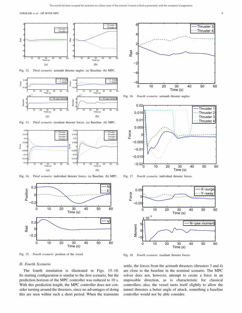
The second simulation scenario was set up so thata thruster turnaround was advantageous assuming that theenvironmental forces remain constant, by initially pointing theazimuth thrusters in the same direction as the environmentalforce (they will thus initially run in reverse to act againstthe environmental force). The baseline controller ends uplocking the azimuth thrusters in the negative direction, whilethe MPC-based one successfully turns them around, as canbe observed in Figs. 8–10. Unlike in the first simulation, theheading remains close to constant in this case because ofincreased penalty for heading deviation. The vessel startedwith zero deviation in heading and along the west–east axis,resulting in motion of the vessel being mostly limited to onedimension. This is somewhat unnatural, but makes it easierto distinguish the various patterns in its movement.

C. Third Scenario

The third scenario is presented in Figs. 11–14. It is morerealistic, starting with the thrusters pointing toward the centerline of the ship, exactly as illustrated in Fig. 3. The resultingconfiguration is well actuated, but, again, the azimuth thrusterspoint in a direction where they have to act in reverse tocounteract the wind force. The MPC controller responds by

Fig. 8. Second scenario: angles of the azimuth thrusters. (a) Baseline.(b) MPC.

Fig. 9. Second scenario: position of the ship. (a) Baseline. (b) MPC.

Fig. 10. Second scenario: resultant thruster forces. (a) Baseline. (b) MPC.

Fig. 11. Third scenario: position of the vessel. (a) Baseline. (b) MPC.

first aligning the azimuth thrusters toward the center line tobring the vessel close to the setpoint as fast as possible. Whenit is well underway about 10 s into the simulation, it startsthe procedure of turning the azimuth thrusters around—aprocedure it carefully coordinates with the position andvelocity of the ship. The result is that at the end of thesimulation, the thrusters point in the optimal direction.Conversely, with the classical controller they continue towork in reverse; this usually requires much higher powerconsumption, twice of that of working in the forward directionwith the parameters chosen for this simulation.



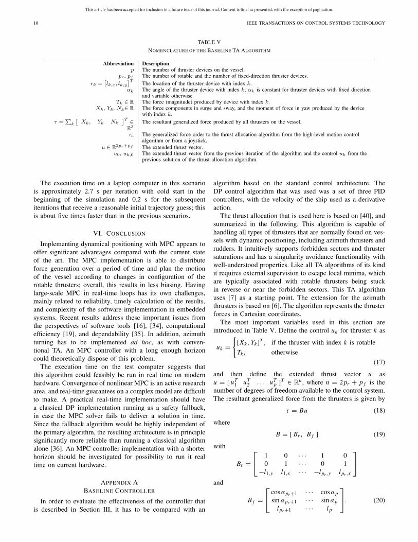
Fig. 12. Third scenario: azimuth thruster angles. (a) Baseline. (b) MPC.

Fig. 13. Third scenario: resultant thruster forces. (a) Baseline. (b) MPC.

Fig. 14. Third scenario: individual thruster forces. (a) Baseline. (b) MPC.

Fig. 15. Fourth scenario: position of the vessel.

D. Fourth Scenario

The fourth simulation is illustrated in Figs. 15–18.Its starting configuration is similar to the first scenario, but theprediction horizon of the MPC controller was reduced to 10 s.With this prediction length, the MPC controller does not con-sider turning around the thrusters, since no advantages of doingthis are seen within such a short period. When the transients

Fig. 16. Fourth scenario: azimuth thruster angles.

Fig. 17. Fourth scenario: individual thruster forces.

Fig. 18. Fourth scenario: resultant thruster forces.

settle, the forces from the azimuth thrusters (thrusters 3 and 4)are close to the baseline in the nominal scenario. The MPCsolver does not, however, attempt to create a force in animpossible direction, as is characteristic for classicalcontrollers; also, the vessel turns itself slightly to allow thetunnel thrusters a better angle of attack, something a baselinecontroller would not be able consider.



TABLE V

NOMENCLATURE OF THE BASELINE TA ALGORITHM

The execution time on a laptop computer in this scenariois approximately 2.7 s per iteration with cold start in thebeginning of the simulation and 0.2 s for the subsequentiterations that receive a reasonable initial trajectory guess; thisis about five times faster than in the previous scenarios.

VI. CONCLUSION

Implementing dynamical positioning with MPC appears tooffer significant advantages compared with the current stateof the art. The MPC implementation is able to distributeforce generation over a period of time and plan the motionof the vessel according to changes in configuration of therotable thrusters; overall, this results in less biasing. Havinglarge-scale MPC in real-time loops has its own challenges,mainly related to reliability, timely calculation of the results,and complexity of the software implementation in embeddedsystems. Recent results address these important issues fromthe perspectives of software tools [16], [34], computationalefficiency [19], and dependability [35]. In addition, azimuthturning has to be implemented ad hoc, as with conven-tional TA. An MPC controller with a long enough horizoncould theoretically dispose of this problem.

The execution time on the test computer suggests thatthis algorithm could feasibly be run in real time on modernhardware. Convergence of nonlinear MPC is an active researcharea, and real-time guarantees on a complex model are difficultto make. A practical real-time implementation should havea classical DP implementation running as a safety fallback,in case the MPC solver fails to deliver a solution in time.Since the fallback algorithm would be highly independent ofthe primary algorithm, the resulting architecture is in principlesignificantly more reliable than running a classical algorithmalone [36]. An MPC controller implementation with a shorterhorizon should be investigated for possibility to run it realtime on current hardware.

APPENDIX ABASELINE CONTROLLER

In order to evaluate the effectiveness of the controller thatis described in Section III, it has to be compared with an

algorithm based on the standard control architecture. TheDP control algorithm that was used was a set of three PIDcontrollers, with the velocity of the ship used as a derivativeaction.

The thrust allocation that is used here is based on [40], andsummarized in the following. This algorithm is capable ofhandling all types of thrusters that are normally found on ves-sels with dynamic positioning, including azimuth thrusters andrudders. It intuitively supports forbidden sectors and thrustersaturations and has a singularity avoidance functionality withwell-understood properties. Like all TA algorithms of its kindit requires external supervision to escape local minima, whichare typically associated with rotable thrusters being stuckin reverse or near the forbidden sectors. This TA algorithmuses [7] as a starting point. The extension for the azimuththrusters is based on [6]. The algorithm represents the thrusterforces in Cartesian coordinates.

The most important variables used in this section areintroduced in Table V. Define the control uk for thruster k as

uk ={[Xk,Yk ]T , if the thruster with index k is rotable

Tk, otherwise

(17)

and then define the extended thrust vector u asu = [ uT

1 uT2 . . . uT

p ]T ∈ Rn , where n = 2 pr + p f is the

number of degrees of freedom available to the control system.The resultant generalized force from the thrusters is given by

τ = Bu (18)

where

B = [ Br , B f ] (19)

with

Br =⎡⎣

1 0 · · · 1 00 1 · · · 0 1−l1,y l1,x · · · −l pr ,y l pr ,x

⎤⎦

and

B f =⎡⎣

cosαpr+1 · · · cosαp

sin αpr+1 · · · sin αp

l pr+1 · · · l p

⎤⎦. (20)



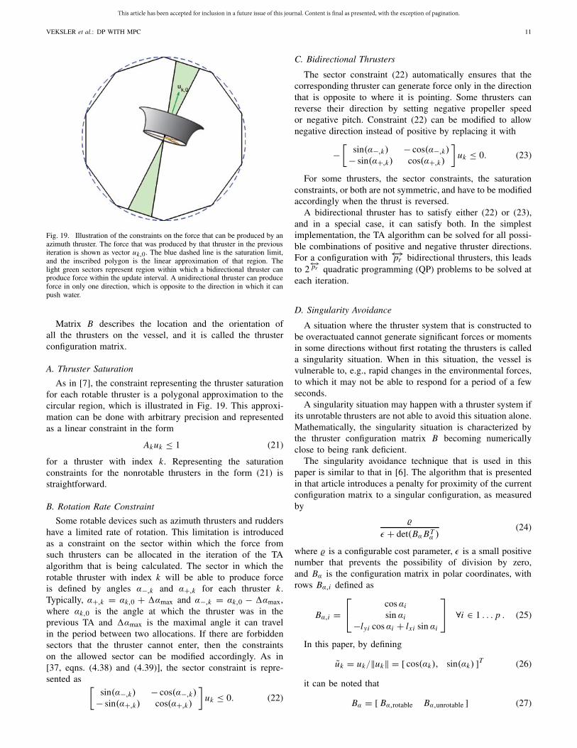
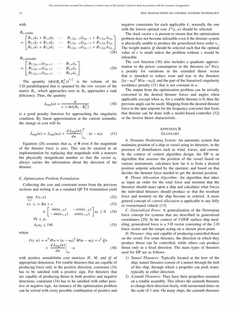
Fig. 19. Illustration of the constraints on the force that can be produced by anazimuth thruster. The force that was produced by that thruster in the previousiteration is shown as vector uk,0. The blue dashed line is the saturation limit,and the inscribed polygon is the linear approximation of that region. Thelight green sectors represent region within which a bidirectional thruster canproduce force within the update interval. A unidirectional thruster can produceforce in only one direction, which is opposite to the direction in which it canpush water.

Matrix B describes the location and the orientation ofall the thrusters on the vessel, and it is called the thrusterconfiguration matrix.

A. Thruster Saturation

As in [7], the constraint representing the thruster saturationfor each rotable thruster is a polygonal approximation to thecircular region, which is illustrated in Fig. 19. This approxi-mation can be done with arbitrary precision and representedas a linear constraint in the form

Akuk ≤ 1 (21)

for a thruster with index k. Representing the saturationconstraints for the nonrotable thrusters in the form (21) isstraightforward.

B. Rotation Rate Constraint

Some rotable devices such as azimuth thrusters and ruddershave a limited rate of rotation. This limitation is introducedas a constraint on the sector within which the force fromsuch thrusters can be allocated in the iteration of the TAalgorithm that is being calculated. The sector in which therotable thruster with index k will be able to produce forceis defined by angles α−,k and α+,k for each thruster k.Typically, α+,k = αk,0 + �αmax and α−,k = αk,0 − �αmax,where αk,0 is the angle at which the thruster was in theprevious TA and �αmax is the maximal angle it can travelin the period between two allocations. If there are forbiddensectors that the thruster cannot enter, then the constraintson the allowed sector can be modified accordingly. As in[37, eqns. (4.38) and (4.39)], the sector constraint is repre-sented as [

sin(α−,k) − cos(α−,k)− sin(α+,k) cos(α+,k)

]uk ≤ 0. (22)

C. Bidirectional Thrusters

The sector constraint (22) automatically ensures that thecorresponding thruster can generate force only in the directionthat is opposite to where it is pointing. Some thrusters canreverse their direction by setting negative propeller speedor negative pitch. Constraint (22) can be modified to allownegative direction instead of positive by replacing it with

−[


]uk ≤ 0. (23)

For some thrusters, the sector constraints, the saturationconstraints, or both are not symmetric, and have to be modifiedaccordingly when the thrust is reversed.

A bidirectional thruster has to satisfy either (22) or (23),and in a special case, it can satisfy both. In the simplestimplementation, the TA algorithm can be solved for all possi-ble combinations of positive and negative thruster directions.For a configuration with←→pr bidirectional thrusters, this leadsto 2←→pr quadratic programming (QP) problems to be solved at

each iteration.

D. Singularity Avoidance

A situation where the thruster system that is constructed tobe overactuated cannot generate significant forces or momentsin some directions without first rotating the thrusters is calleda singularity situation. When in this situation, the vessel isvulnerable to, e.g., rapid changes in the environmental forces,to which it may not be able to respond for a period of a fewseconds.

A singularity situation may happen with a thruster system ifits unrotable thrusters are not able to avoid this situation alone.Mathematically, the singularity situation is characterized bythe thruster configuration matrix B becoming numericallyclose to being rank deficient.

The singularity avoidance technique that is used in thispaper is similar to that in [6]. The algorithm that is presentedin that article introduces a penalty for proximity of the currentconfiguration matrix to a singular configuration, as measuredby

�

ε + det(BαBTα )

(24)

where � is a configurable cost parameter, ε is a small positivenumber that prevents the possibility of division by zero,and Bα is the configuration matrix in polar coordinates, withrows Bα,i defined as

Bα,i =⎡⎣

cosαi

sin αi

−lyi cosαi + lxi sin αi

⎤⎦ ∀i ∈ 1 . . . p . (25)

In this paper, by defining

uk = uk/‖uk‖ = [ cos(αk), sin(αk) ]T (26)

it can be noted that

Bα = [ Bα,rotable Bα,unrotable ] (27)



with

Bα,rotable

=⎡⎣

B1,1u1 + B1,2u2 · · · B1,2pr−1u2pr−1 + B1,2pr u2pr



⎤⎦

(28)

Bα,unrotable

=⎡⎣

B1,2pr+1u2pr+1 · · · B1,nun

B2,2pr+1u2pr+1 · · · B2,nun

B3,2pr+1u2pr+1 · · · B3,nun

⎤⎦. (29)

The quantity (det(BαBTα ))

1/2is the volume of the

3-D parallelepiped that is spanned by the row vectors of thematrix Bα, which approaches zero as Bα approaches a rankdeficiency. Thus, the quantity

Jsing(u) = �

ε + det(Bα · BT

α

) (30)

is a good penalty function for approaching the singularitycondition. By linear approximation at the current azimuths,the change in cost will be

Jsing(u) = Jsing(u0)+ d Jsing(u)

du

∣∣∣∣T

uo

· (u − u0). (31)

Equation (26) assumes that uk = 0 even if the magnitudeof the thruster force is zero. This can be ensured in animplementation by replacing that magnitude with a nonzerobut physically insignificant number so that the vector uk

always carries the information about the direction of thethruster.

E. Optimization Problem Formulation

Collecting the cost and constraint terms from the previoussections and writing it as a standard QP TA formulation yield

minu,s

J (s, u) (32)

s.t. τc = Bu + s (33)

±[


]uk ≤ 0 (34)

∀k ≤ pr

Akuk ≤ 1∀k (35)

where

J (s, u) = uT H u + (u − u0)T M(u − u0)+ sT Qs

+ d Jsing(u)

du

∣∣∣∣u0

· u (36)

with positive semidefinite cost matrices H , M , and Q ofappropriate dimension. For rotable thrusters that are capable ofproducing force only in the positive direction, constraint (34)has to be satisfied with a positive sign. For thrusters thatare capable of producing thrust in both positive and negativedirections, constraint (34) has to be satisfied with either posi-tive or negative sign. An instance of the optimization problemcan be solved with every possible combination of positive and

negative constraints for each applicable k; normally the onewith the lowest optimal cost J ∗(s, u) should be selected.

The slack vector s is present to ensure that the optimizationproblem does not become infeasible even if the thruster systemis physically unable to produce the generalized force order τc.The weight matrix Q should be selected such that the optimalvalue of s is small unless the problem without s would beinfeasible.

The cost function (36) also includes a quadratic approxi-mation to the power consumption in the thrusters (uT H u),a penalty for variations in the extended thrust vectorthat is intended to reduce wear and tear in the thrusters[(u−u0)

T M(u−u0)], and the part of the linearized singularityavoidance penalty (31) that is not constant in u.

The output from the optimization problem can be triviallyconverted to the desired thruster forces and angles whenapplicable (except when uk for a rotable thruster is 0, then theprevious angle can be used). Mapping from the desired thrusterforce to the rpm setpoint for the frequency converter that feedsthat thruster can be done with a model-based controller [32]or the inverse thrust characteristic.

APPENDIX BGLOSSARY

A. Dynamic Positioning System: An automatic system thatmaintains position of a ship or vessel using its thrusters, in thepresence of disturbances such as wind, waves, and current.In the context of control algorithm design, the DP is analgorithm that assesses the position of the vessel based onvarious instruments, calculates how far it is from a desiredposition setpoint selected by the operator, and based on thatdecides the thruster force needed to get the desired position.

B. Thrust Allocation Algorithm: An algorithm that takesas input an order for the total force and moment that thethrusters should enact upon a ship and calculates what forcesthe individual thrusters should produce so that the resultantforce and moment on the ship become as ordered. A moregeneral concept of control allocation is applicable to any fullyor overactuated vehicle [13].

C. Generalized Force: A generalization of the Newtonianforce concept for systems that are described in generalizedcoordinates [29]. In the context of 3-DOF surface ship mod-eling, generalized force is a 3-D vector consisting of the 2-Dforce vector and the torque acting on a chosen pivot point.

D. Thruster: Any unit capable of producing controlled thruston the vessel. For some thrusters, the direction in which theyproduce thrust can be controlled, while others can producethrust only in a fixed direction. The main types of thrustersused for DP are as follows.

1) Tunnel Thrusters: Typically located at the bow of theship, tunnel thrusters consist of a tunnel through the hullof this ship, through which a propeller can push water,typically in either direction.

2) Azimuth Thrusters: They have their propellers mountedon a rotable assembly. This allows the azimuth thrustersto change their direction freely, with turnaround times onthe scale of 1 min. On many ships, the azimuth thrusters



are not allowed to push water in certain directions, suchas against other thrusters or at other critical machinery.This type of thruster is typically located at the aft of theship or beneath the columns of semisubmersible rigs.

3) Ruddered or Unruddered Propellers: They are classicalpropellers, typically located at the aft of the ship andpointing backward. They are often mechanically pow-ered through a drive shaft. A rudder is most effectivewhen a propeller pushes water that passes its surface,which is typically behind the propeller. Rudders aretherefore often installed behind propellers to allow gen-erating a sideways force at the location of the rudder,which also normally creates a yaw moment on the ship.

E. Thruster Biasing: Deliberately increasing the power con-sumption in the thrusters without changing the total producedforce and moment on the ship, essentially making the thrusterswork against one another.

For a given azimuth and rudder angle vector α, the com-bined force vector and angular momentum produced by thethrusters is

τ = B(α) f (37)

and is a linear combination of the forces f generated by theindividual thrusters. If there are four or more thrusters on boardthe ship, then matrix B(α) is guaranteed to have a nontrivialnull space F0. In addition, if f ∗ is a strict global minimizer ofthe power consumption for a given τ , then for any f0 ∈ F0 \0,the power consumption for f ∗ + f0 will be higher thanfor f ∗, with the resultant generalized force remaining thesame. Therefore, biasing can always be achieved as longas there are at least four nonsaturated thrusters availablefor the purpose. Fewer than four thrusters are sufficient forconfigurations in which the columns of the matrix B(α) arenot independent.

A. Wave Filter

Waves characteristically induce a cyclic high-frequencyback-and-forth motion on ships. Compensating for the wave-induced motions would demand large power expenditure andincreased wear and tear. For this reason, the cyclic wave-induced motions of the vessel are usually allowed to runtheir course, without interference from the DP system. Thisis implemented by passing the position reference through awave filter algorithm, which calculates what the position ofthe vessel would have been without the cyclic wave-inducedmotions. Several methods for implementing such a filter havebeen proposed [2], [38], [39].

ACKNOWLEDGMENT

The authors would like to thank S. Vichik and T. Kelmanof University of California Berkeley and A. Sørensen ofNorwegian University of Science and Technology for thediscussions and advice.

REFERENCES

[1] (Jul. 2011). Rules for Classification of Ships, DNV GL Standard Part 6Chapter 7, Dynamic Positioning Systems. [Online]. Available:https://exchange.dnv.com/publishing/RulesShip/2011-01/ts607.pdf

[2] T. I. Fossen, Handbook of Marine Craft Hydrodynamics and MotionControl. New York, NY, USA: Wiley, Apr. 2011.

[3] O. G. Hvamb, “A new concept for fuel tight DP control,” in Proc. Dyn.Positioning Conf., Houston, TX, USA, Sep. 2001, pp. 1–10.

[4] H. Chen, L. Wan, F. Wang, and G. Zhang, “Model predictivecontroller design for the dynamic positioning system of a semi-submersible platform,” J. Marine Sci. Appl., vol. 11, no. 3, pp. 361–367,Sep. 2012.

[5] S. P. Berge and T. I. Fossen, “Robust control allocation of overactu-ated ships; experiments with a model ship,” in Proc. 4th IFAC Conf.Manoeuvring Control Marine Craft, 1997, pp. 166–171.

[6] T. A. Johansen, T. I. Fossen, and S. P. Berge, “Constrained nonlinearcontrol allocation with singularity avoidance using sequential quadraticprogramming,” IEEE Trans. Control Syst. Technol., vol. 12, no. 1,pp. 211–216, Jan. 2004.

[7] T. A. Johansen, T. P. Fuglseth, P. Tøndel, and T. I. Fossen, “Optimalconstrained control allocation in marine surface vessels with rudders,”Control Eng. Pract., vol. 16, no. 4, pp. 457–464, Apr. 2008.

[8] B. Realfsen, “Reducing NOx emission in DP2 and DP3 operations,”Conference Dyn. Positioning Conf., 2009.

[9] E. Mathiesen, B. Realfsen, and M. Breivik, “Methods for reducing fre-quency and voltage variations on DP vessels,” in Proc. Dyn. PositioningConf., Oct. 2012, pp. 1–11.

[10] A. Veksler, T. A. Johansen, and R. Skjetne, “Thrust allocation withpower management functionality on dynamically positioned vessels,” inProc. Amer. Control Conf., Jun. 2012, pp. 1468–1475.

[11] A. Veksler, T. A. Johansen, and R. Skjetne, “Transient power controlin dynamic positioning—Governor feedforward and dynamic thrustallocation,” in Proc. 9th IFAC Conf. Manoeuvring Control Marine Craft,2012, pp. 158–163.

[12] D. Radan, A. J. Sørensen, A. K. Ådnanes, and T. A. Johansen, “Reducingpower load fluctuations on ships using power redistribution control,”J. Marine Technol., vol. 45, no. 3, pp. 162–174, Jul. 2008.

[13] T. A. Johansen and T. I. Fossen, “Control allocation—A survey,”Automatica, vol. 49, no. 5, pp. 1087–1103, May 2013.

[14] J. B. Rawlings, “Tutorial overview of model predictive control,” IEEEControl Syst., vol. 20, no. 3, pp. 38–52, Jun. 2000.

[15] D. Q. Mayne, J. B. Rawlings, C. V. Rao, and P. O. M. Scokaert,“Constrained model predictive control: Stability and optimality,”Automatica, vol. 36, no. 6, pp. 789–814, Jun. 2000. [Online]. Available:http://www.sciencedirect.com/science/article/pii/S0005109899002149

[16] B. Houska, H. J. Ferreau, and M. Diehl, “An auto-generated real-time iteration algorithm for nonlinear MPC in the microsecond range,”Automatica, vol. 47, no. 10, pp. 2279–2285, Oct. 2011.

[17] B. Houska, H. J. Ferreau, and M. Diehl, “ACADO toolkit an open sourceframework for automatic control and dynamic optimization,” OptimalControl Appl. Methods, vol. 32, no. 3, pp. 298–312, 2011.

[18] Y. Wang and S. Boyd, “Fast model predictive control using onlineoptimization,” IEEE Trans. Control Syst. Technol., vol. 18, no. 2,pp. 267–278, Mar. 2010.

[19] D. K. M. Kufoalor, S. Richter, L. Imsland, T. A. Johansen, M. Morari,and G. O. Eikrem, “Embedded model predictive control on a PLC usinga primal-dual first-order method for a subsea separation process,” inProc. Medit. Conf. Control Autom. (MED), Palermo, Italy, Jun. 2014,pp. 368–373.

[20] J. F. Hansen, “Modelling and control of marine power systems,”Ph.D. dissertation, Dept. Eng. Cybern., Norwegian Univ. Sci. Technol.,Trondheim, Norway, 2000.

[21] T. I. Bø, “Dynamic model predictive control for load sharing in electricpower plants for ships,” M.S. thesis, Dept. Marine Technol., NorwegianUniv. Sci. Technol., Trondheim, Norway, 2012.

[22] T. I. Bø and T. A. Johansen, “Scenario-based fault-tolerant modelpredictive control for diesel-electric marine power plant,” in Proc.MTS/IEEE OCEANS, Jun. 2013, pp. 1–5.

[23] A. Veksler, T. A. Johansen, E. Mathiesen, and R. Skjetne,“Governor principle for increased safety and economy on vessels withdiesel-electric propulsion,” in Proc. Eur. Control Conf., Jul. 2013,pp. 2579–2584.

[24] Y. Luo, A. Serrani, S. Yurkovich, D. B. Doman, and M. W. Oppenheimer,“Model predictive dynamic control allocation with actuator dynamics,”in Proc. Amer. Control Conf., Boston, MA, USA, Jun./Jul. 2004,pp. 1695–1700.

[25] M. Hanger, T. A. Johansen, G. K. Mykland, and A. Skullestad,“Dynamic model predictive control allocation using CVXGEN,” in Proc.9th IEEE Int. Conf. Control Autom. (ICCA), Santiago, Chile, Dec. 2011,pp. 417–422.



[26] T. A. Johansen, A. J. Sørensen, O. J. Nordahl, O. Mo, andT. I. Fossen, “Experiences from hardware-in-the-loop (HIL) testing ofdynamic positioning and power management systems,” in Proc. OSV,Singapore, 2007.

[27] L. Grüne and J. Pannek, Nonlinear Model Predictive Control: Theoryand Algorithms (Communications and Control Engineering), 1st ed.New York, NY, USA: Springer-Verlag, 2011. [Online]. Available:http://www.springer.com/978-0-85729-500-2

[28] Nomenclature for Treating the Motion of a Submerged BodyThrough a Fluid, Technical and Research Bulletin No. 1-5,The Society of Naval Architects and Marine Engineers,Technical and Research Committee, 1950. [Online]. Available:http://www.itk.ntnu.no/fag/gnc/papers/Sname%201950.PDF

[29] H. Goldstein, C. P. Poole, Jr., and J. L. Safko, Classical Mechanics.Reading, MA, USA: Addison-Wesley, Jun. 2001.

[30] F. M. White, Fluid Mechanics. New York, NY, USA: McGraw-Hill,2003.

[31] J. D. van Manen and P. van Oossanen, “Propulsion,” in Principlesof Naval Architecture, E. V. Lewis, Ed. Jersey City, NJ, USA:SNAME, 1988, ch. 6. [Online]. Available: http://maritimesun.com/news/wp-content/uploads/2012/03/principles-of-naval-architecture-vol-2-resistance-propulsion-vibration.pdf

[32] L. Pivano, T. A. Johansen, and O. N. Smogeli, “A four-quadrant thrustestimation scheme for marine propellers: Theory and experiments,”IEEE Trans. Control Syst. Technol., vol. 17, no. 1, pp. 215–226,Jan. 2009.

[33] T. I. Fossen, Marine Control Systems. Trondheim, Norway: TapirTrykkeri, 2002.

[34] D. K. M. Kufoalor, B. J. T. Binder, H. J. Ferreau, L. Imsland,T. A. Johansen, and M. Diehl, “Automatic deployment of industrialembedded model predictive control using qpOASES,” in Proc. Eur.Control Conf., Linz, Austria, 2015, pp. 1–8.

[35] T. A. Johansen, “Toward dependable embedded model predictive con-trol,” IEEE Syst. J., to be published.

[36] A. Burns and A. Wellings, Real-Time Systems and ProgrammingLanguages, 3rd ed. Reading, MA, USA: Addison-Wesley,2001.

[37] E. Ruth, “Propulsion control and thrust allocation on marine vessels,”Ph.D. dissertation, Dept. Marine Technol., Norwegian Univ. Sci.Technol., Trondheim, Norway, 2008.

[38] M. J. Grimble, R. J. Patton, and D. A. Wise, “The design of dynamicship positioning control systems using stochastic optimal controltheory,” Optim. Control Appl. Methods, vol. 1, no. 2, pp. 167–202,Apr./Jun. 1980. [Online]. Available: http://dx.doi.org/10.1002/oca.4660010207

[39] V. Hassani, A. J. Sorensen, A. M. Pascoal, and A. P. Aguiar,“Multiple model adaptive wave filtering for dynamic positioning ofmarine vessels,” in Proc. Amer. Control Conf. (ACC), Jun. 2012,pp. 6222–6228.

[40] A. Veksler, T. A. Johansen, F. Borrelli, and B. Realfsen, “Cartesian thrustallocation algorithm with variable direction thrusters, turn rate limitsand singularity avoidance,” in Proc. IEEE MultiConf. Syst. Control,2014.

Aleksander Veksler (M’–) was born in 1982.He received the M.Sc. degree in engineering cyber-netics and the Ph.D. degree from the NorwegianUniversity of Science and Technology, Trondheim,Norway, in 2009 and 2014, respectively.

He was a Research Visitor to the University ofCalifornia at San Diego, San Diego, CA, USA,in 2008/2009, while working on his master’s thesis,and to the University of California at Berkeley,Berkeley, CA, USA, in 2013/2014, while working onhis Ph.D. thesis. He is currently a Project Engineer

with Step Solutions, Oslo, Norway, where he is involved in the developmentof ballast water treatment systems.

Tor Arne Johansen (SM’–) was born in 1966.He received the M.Sc. and Ph.D. degrees in electri-cal and computer engineering from the NorwegianUniversity of Science and Technology (NTNU),Trondheim, Norway, in 1989 and 1994, respectively.

He was with SINTEF Electronics and Cybernetics,Oslo, Norway, as a Researcher, before he wasappointed as an Associate Professor of EngineeringCybernetics with NTNU in 1997 and was promotedto Professor in 2001. He was a Research Visitor withthe University of Southern California, Los Angeles,

CA, USA, the Delft University of Technology, Delft, The Netherlands, andthe University of California at San Diego, San Diego, CA, USA. In 2002,he co-founded Marine Cybernetics AS, Oslo, where he was the Vice Presidentuntil 2008. He has supervised over ten Ph.D. students, holds several patents,and has directed numerous research projects. He is currently a PrincipalResearcher with the Center of Excellence on Autonomous Marine Operationsand Systems, NTNU. He has authored over 100 articles in internationaljournals and numerous conference articles and book chapters in nonlinearcontrol and estimation, optimization, adaptive control, and model predictivecontrol with applications in the marine, automotive, biomedical, and processindustries.

Prof. Johansen received the 2006 SAE Arch T. Colwell Merit Award.

Francesco Borrelli (SM’–) received the Laureadegree in computer science engineering from theUniversity of Naples Federico II, Naples, Italy,in 1998, and the Ph.D. degree from the Auto-matic Control Laboratory, ETH Zurich, Zurich,Switzerland, in 2002.

He is currently an Associate Professor with theDepartment of Mechanical Engineering, Universityof California at Berkeley, Berkeley, CA, USA.He has authored over 100 publications in predictivecontrol and the book entitled Constrained Optimal

Control of Linear and Hybrid Systems (Springer Verlag). His current researchinterests include constrained optimal control, model predictive control andits application to advanced automotive control, and energy efficient buildingoperation.

Prof. Borrelli was the winner of the 2009 NSF CAREER Award and the2012 IEEE Control System Technology Award.

Bjørnar Realfsen received the M.Sc. degree inmathematical modeling from the Institute of Infor-matics, University of Oslo, Oslo, Norway, in 1998.

He has been with Kongsberg Maritime,Kongsberg, Norway. He has been a majorcontributor in the development of applications forthrust allocation in dynamic positioning systemswith power limitations or power demands. He iscurrently a Principal Engineer with the Product andDevelopment Department for Dynamic PositioningSystems, Kongsberg Maritime. His current research

interests include thrust allocation and guidance and control.Mr. Realfsen’s work has been presented at the MTS DP Conference

in 2006, 2009, and 2012.

IEEE TRANSACTIONS ON CONTROL SYSTEMS TECHNOLOGY 1 Dynamic ...frborrel/pdfpub/Alex2016.pdf ·...

Documents

Transcript of IEEE TRANSACTIONS ON CONTROL SYSTEMS TECHNOLOGY 1 Dynamic ...frborrel/pdfpub/Alex2016.pdf ·...