IEEE Trans. Pattern Analysis and Machine Intelligence 1983 ...

tion,” IEEE Trans. Pattern Analysis and Machine Intelligence, PAMI-5,4, July1983.

[15] Bolles, R.C. and Horaud, P., “3DPO: A three-dimensional part orientation sys-tem,” in Three-Dimensional Machine Vision, Kluwer, Boston, MA, 1987.

[16] Koenderink, J.J. and Van Doorn, A.J., “The Singularities of the Visual Mapping,”Biological Cybernetics, 24(1), 1976

[17] Chin, R.T. and Dyer, C.R. “Model-based recognition in robot vision” ,ACM Com-puting Surveys, 18(1), 1986.

Reference

[1] Gauss, K. F.,General Investigations of Curved Surfaces, Raven Press, New York,1965.

[2] Lysternik, L.A., Convex Figures and Polyhedra, Dover Publications, New York,1963.

[3] Horn, B.K.P., “Extended Gaussian Image,”Proc. of IEEE, Vol. 72, No. 12,pp.1671-1686, December 1984.

[4] Ikeuchi, K., “Recognition of 3-D Objects using the Extended Gaussian Image,”Proc. of Intern. Joint Conf on Artificial Intelligence, Vancouver, B.C., pp.595-600,August 1981.

[5] Brou, P., “Using the Gaussian Image to Find the Orientation of Objects,” Intern.Journal of Robotics Research, Vol. 3, No. 4, pp. 89-125, Winter 1984.

[6] Little, J. J., “Determining Object Attitude from Extended Gaussian Image,”Proc.of Intern. Joint Conf on Artificial Intelligence, Los Angeles, California, pp. 960-963, August 1985.

[7] Ikeuchi, K. and Horn, B.K.P., “Picking up an Object from a Pile of Objects,” inRobotics Research:The First International Symposium, J. M. Brady & R. Paul(eds.), MIT Press, Cambridge, Massachusetts, pp. 139-162, 1984.

[8] Kang, S.B. and Ikeuchi, K., “The Complex EGI: New Representation for 3-D PoseDetermination,” IEEE Trans Pattern Analysis and Machine Intelligence, Vol. 15,No. 7, pp. 707-721, July 1993.

[9] Nalwa, V. S., “Representing Oriented Piecewise C2 Surfaces,”Proc. 2nd Intern.Conf. on Computer Vision, pp. 40-51, December 1988.

[10] Roach, J. W. Wright, J.S., and Ramesh, V., “Sperical Dual Images: A 3-D Repre-sentation Method for Solid Objects that Combines Dual Space and GaussianSphere,”Proc. IEEE Conf on Computer Vision and Pattern Recognition, pp. 236-241, June 1986.

[11] Dellingette, H., Hebert, M., and Ikeuchi, K., “A Spherical Representation for theRecognition of Curved Objects,”Proc. Intern. Conf on Computer Vision, pp.103-112, May 1993.

[12] Besl, P. and Kay, N.D., “A Method for Registeration of 3-D Shapes,” IEEE TransPatern Analysis Machine Intelligence, Vol. 14, No.2, Feb 1992.

[13] Higuchi, K. Delingette, H. Hebert, M. and Ikeuchi, K., “Merging Multiple Viewsusing a Spherical Representation,”Proc. IEEE Workshop on CAD-based Vision,pp.124-131, Feb 1993.

[14] Oshima, M. and Shirai, Y., “Object recognition using three-dimensional informa-

Acknowledgments

The research described in this paper was done with our former and current students, Dr.

Sing Bing Kang of DEC Cambridge Research Lab, Dr. Herve Delingette of INRIA Sophia-

Antipolis, Dr. Kazunori Higuchi of Toyota Central Research Lab, and Harry Shum of

CMU.. Their contributions are greatly appreciated.

4. Conclusion

In this paper, we argued that main issue in representing general objects is to be able to define

an intrinsic coordinate system on a surface, onto which properties such as curvature may be

mapped. A convenient way of addressing this problem is to define an intrinsic mapping

between a closed surface and the unit sphere.

Although we are still far from a completely satisfactory solution, we have made significant

progress. Starting with the EGI, which can only handle convex objects under rotation, we

have introduced the DEGI and the CEGI which can deal with translations and, to some

extent, with non-convexity.

Finally, the SAI relaxes many of the constraints of the EGI-like representations by preserv-

ing the connectiviy of the surface, that is, a connected path on the surface maps to a con-

nected path on the sphere. This property allows us to deal with non-convex objects and with

general transformations.

We are still a long way from a general solution, however. First of all, the SAI is limited to

objects with a genus 0 topology. Second, the algorithm used for extracting the underlying

deformable surface does have limitations with respect to the variation in the object shape.

Nevertheless, we believe that intrinsic coordinate maps are a fundamental tool for general

object matching and we working toward improving the SAI to handle more general cases.

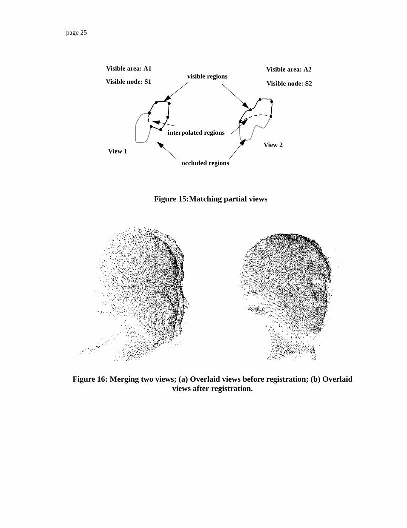
Figure 15:Matching partial views

visible regions

occluded regions

interpolated regions

View 1

Visible area: A1 Visible area: A2

Visible node: S1 Visible node: S2

View 2

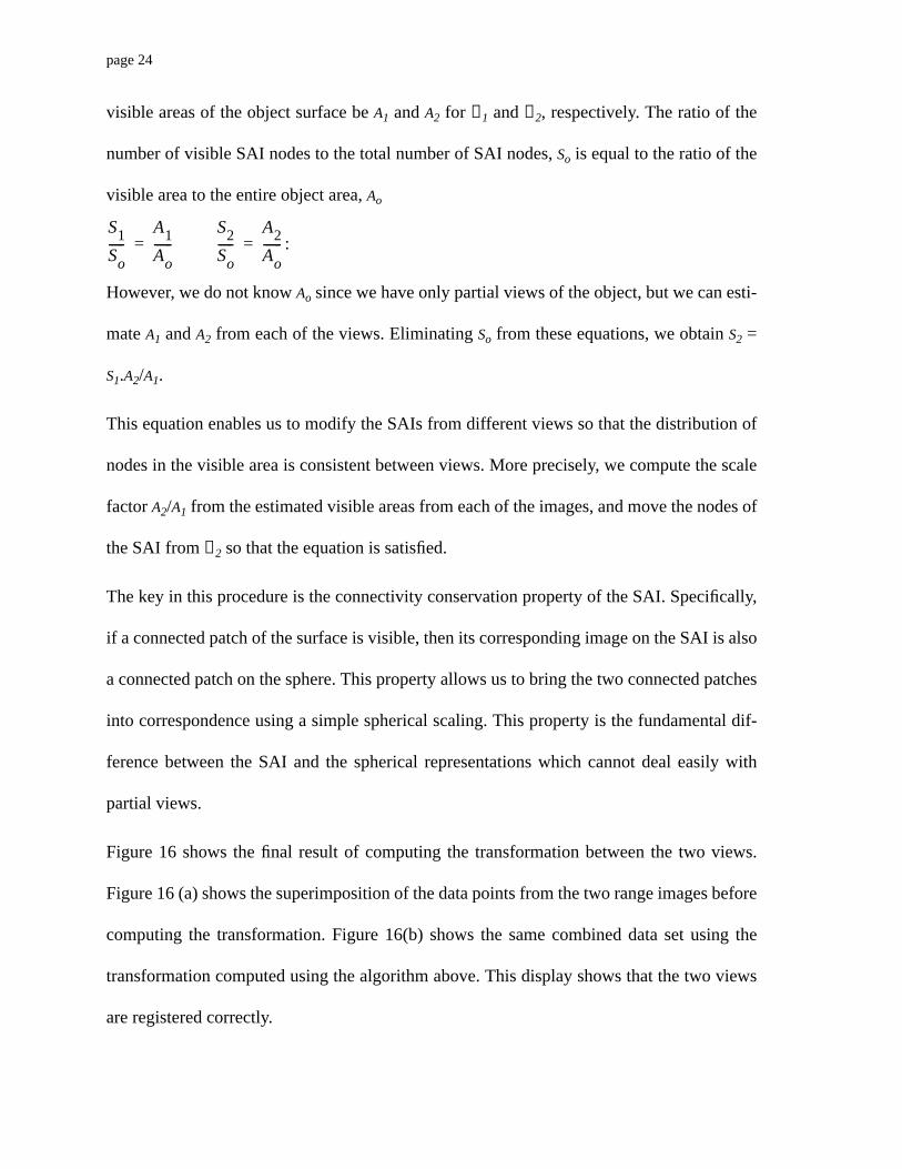
Figure 16: Merging two views; (a) Overlaid views before registration; (b) Overlaidviews after registration.

visible areas of the object surface beA1 andA2 for V1 andV2, respectively. The ratio of the

number of visible SAI nodes to the total number of SAI nodes,So is equal to the ratio of the

visible area to the entire object area,Ao

:

However, we do not knowAo since we have only partial views of the object, but we can esti-

mateA1 andA2 from each of the views. EliminatingSo from these equations, we obtainS2 =

S1.A2/A1.

This equation enables us to modify the SAIs from different views so that the distribution of

nodes in the visible area is consistent between views. More precisely, we compute the scale

factorA2/A1 from the estimated visible areas from each of the images, and move the nodes of

the SAI fromV2 so that the equation is satisfied.

The key in this procedure is the connectivity conservation property of the SAI. Specifically,

if a connected patch of the surface is visible, then its corresponding image on the SAI is also

a connected patch on the sphere. This property allows us to bring the two connected patches

into correspondence using a simple spherical scaling. This property is the fundamental dif-

ference between the SAI and the spherical representations which cannot deal easily with

partial views.

Figure 16 shows the final result of computing the transformation between the two views.

Figure 16 (a) shows the superimposition of the data points from the two range images before

computing the transformation. Figure 16(b) shows the same combined data set using the

transformation computed using the algorithm above. This display shows that the two views

are registered correctly.

S1

So-----

A1

Ao------=

S2

So-----

A2

Ao------=

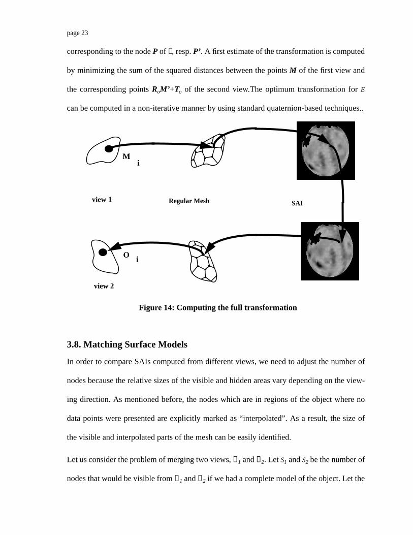
corresponding to the nodeP of S, resp.P’. A first estimate of the transformation is computed

by minimizing the sum of the squared distances between the pointsM of the first view and

the corresponding pointsRoM’ +To of the second view.The optimum transformation forE

can be computed in a non-iterative manner by using standard quaternion-based techniques..

3.8. Matching Surface Models

In order to compare SAIs computed from different views, we need to adjust the number of

nodes because the relative sizes of the visible and hidden areas vary depending on the view-

ing direction. As mentioned before, the nodes which are in regions of the object where no

data points were presented are explicitly marked as “interpolated”. As a result, the size of

the visible and interpolated parts of the mesh can be easily identified.

Let us consider the problem of merging two views,V1 andV2. LetS1 andS2 be the number of

nodes that would be visible fromV1 andV2 if we had a complete model of the object. Let the

Figure 14: Computing the full transformation

Regular Mesh SAI

M

O

i

i

view 1

view 2

The row that produces the minimumDi gives the best correspondence between nodes of the

mesh, {(Pj, P’ ij)}, which is used for computing the full transformation between the object

meshes as described in the next section.

This algorithm is guaranteed to find the global optimum ofD and it does not require an ini-

tial estimate of the transformation. It is efficient because all that is required at run time is to

look up the correspondence table, to compute sum of square differences of corresponding

nodes and to add them up

3.7. Computing the Full Transformation

The last step in matching objects is to derive the transformation between the actual objects,

given the rotation between their SAIs (See Figure 14). The rotational part of the transforma-

tion is denoted byRo, the translational part byTo. Given a SAI rotationR, we know the cor-

responding nodeP’ of each nodeP of S. Let M, resp.M’ , be the point on the view

..

..

..

..P1

P2

P3P4

Pj

P’ij

P’i2P’i3

P’i4

P’i1

PijPi1 PiK

node number

“rot

atio

n”

i

j1 K

num

ber

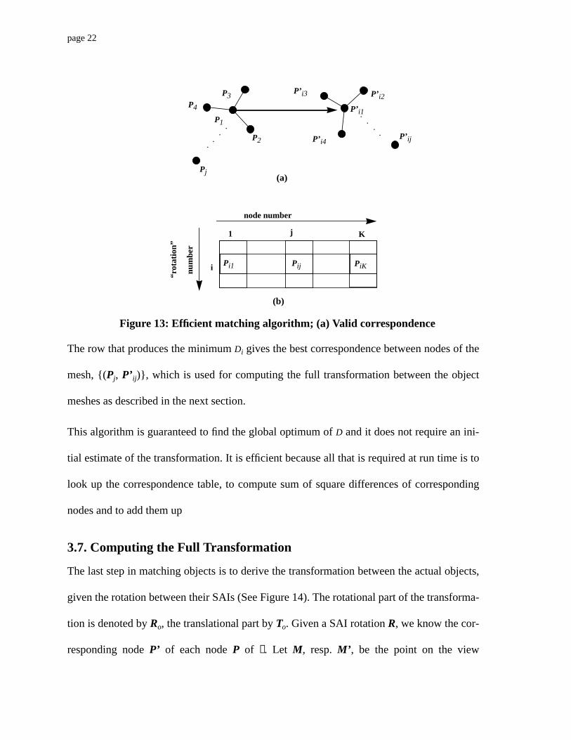
Figure 13: Efficient matching algorithm; (a) Valid correspondence

(a)

(b)

correspondences. Moreover, there is only a small number of such initial correspondences.

Based on this observation, we developed an SAI matching algorithm decomposed into two

stages: a pre-processing phase and a run-time phase. During pre-processing, we generate the

data structure shown in Figure 13(b). The data structure is a two dimensional array in which

each row corresponds to a possible rotation of the SAI and in which columnj of row i is the

index of the nodePij corresponding to nodePj and correspondence numberi. At run-time,

the distance is evaluated for each row of the array:

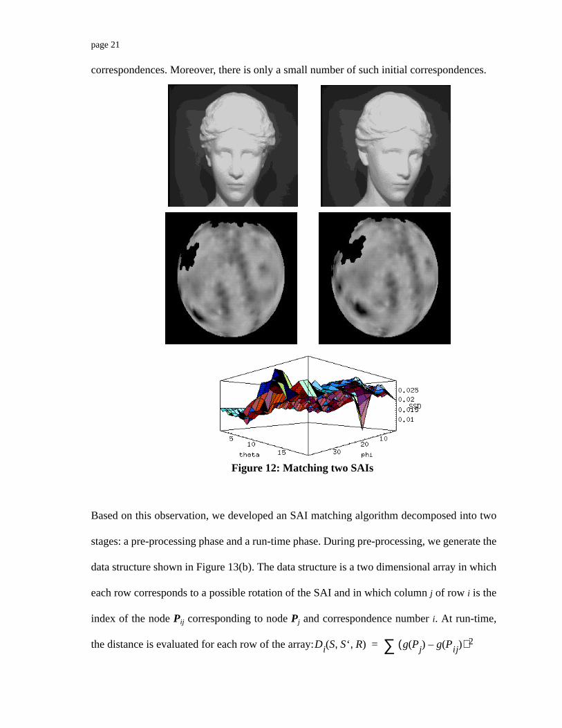
Figure 12: Matching two SAIs

Di S S‘ R, ,( ) g Pj( ) g Pij( )–( ) 2∑=

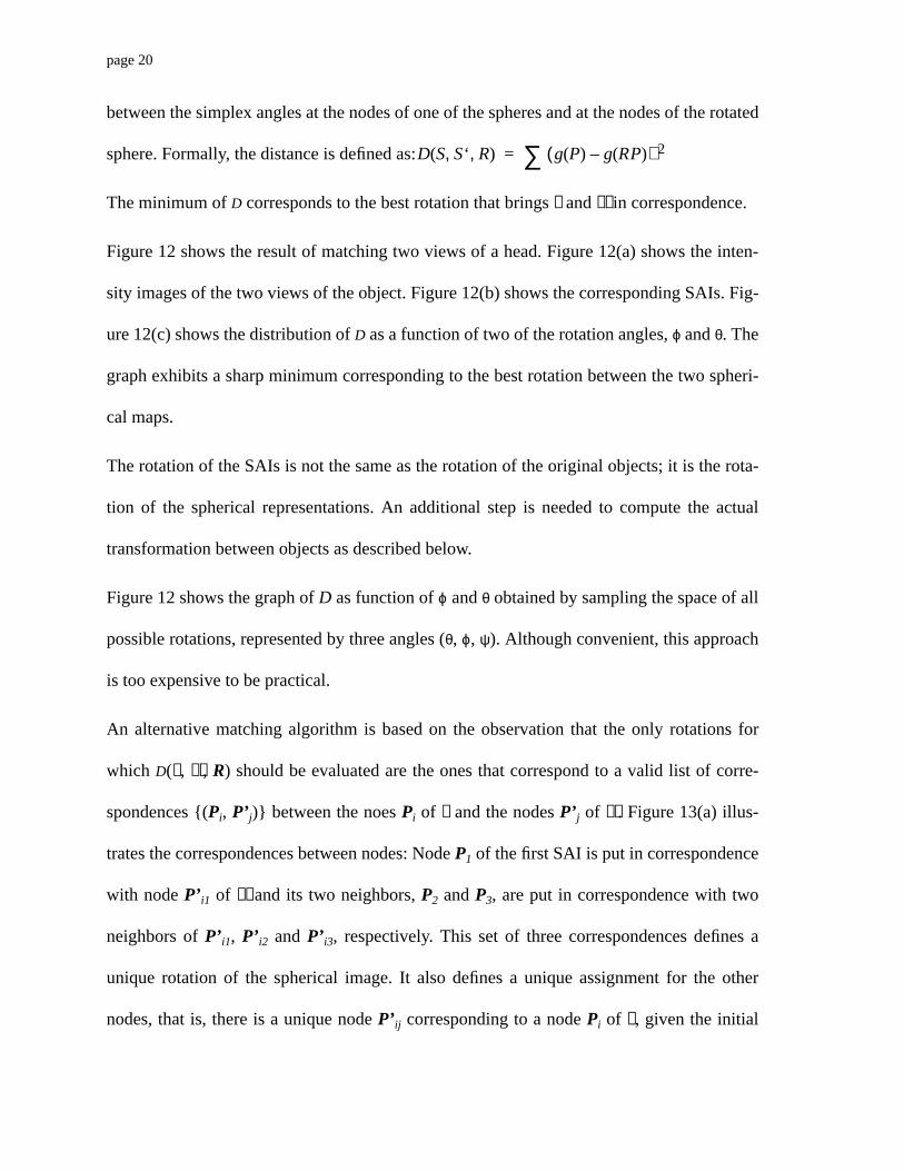
between the simplex angles at the nodes of one of the spheres and at the nodes of the rotated

sphere. Formally, the distance is defined as:

The minimum ofD corresponds to the best rotation that bringsS andS’ in correspondence.

Figure 12 shows the result of matching two views of a head. Figure 12(a) shows the inten-

sity images of the two views of the object. Figure 12(b) shows the corresponding SAIs. Fig-

ure 12(c) shows the distribution ofD as a function of two of the rotation angles,ϕ andθ. The

graph exhibits a sharp minimum corresponding to the best rotation between the two spheri-

cal maps.

The rotation of the SAIs is not the same as the rotation of the original objects; it is the rota-

tion of the spherical representations. An additional step is needed to compute the actual

transformation between objects as described below.

Figure 12 shows the graph ofD as function ofϕ andθ obtained by sampling the space of all

possible rotations, represented by three angles (θ, ϕ, ψ). Although convenient, this approach

is too expensive to be practical.

An alternative matching algorithm is based on the observation that the only rotations for

which D(S, S’, R) should be evaluated are the ones that correspond to a valid list of corre-

spondences {(Pi, P’ j)} between the noesPi of S and the nodesP’ j of S’. Figure 13(a) illus-

trates the correspondences between nodes: NodeP1 of the first SAI is put in correspondence

with nodeP’ i1 of S’ and its two neighbors,P2 andP3, are put in correspondence with two

neighbors ofP’ i1, P’ i2 andP’ i3, respectively. This set of three correspondences defines a

unique rotation of the spherical image. It also defines a unique assignment for the other

nodes, that is, there is a unique nodeP’ ij corresponding to a nodePi of S, given the initial

D S S‘ R, ,( ) g P( ) g RP( )–( ) 2∑=

3.6. Matching Surface Models

We now address the matching problem: Given two SAIs, determine the rotation between

them, and then find the rigid transformation between the two original sets of points. The rep-

resentations of a single object with respect to two different viewing directions are related by

a rotation of the underlying sphere. Therefore, the most straightforward approach is to com-

pute a distance measure between two SAIs. Once the rotation yielding minimum distance is

determined, the full 3-D transformation can be determined.

In the following discussion, we will consider only the vertices of the SAIs that correspond to

visible parts of the surface. LetS andS’ be the SAIs of two views.S andS’ are representa-

tions of the same area of the object if there exists a rotationR such thatg(P) = g (RP) for

every pointP of S.

The problem now is to find this rotation using the discrete representation ofS andS’. This is

done by defining a distanceD(S, S’, R) between SAIs as the sum of squared differences

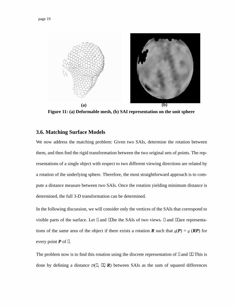
Figure 11: (a) Deformable mesh, (b) SAI representation on the unit sphere(a) (b)

transformations.

3) A connected patch of the surface maps to a connected patch of the spherical image. It is

this property that allows us to work with non-convex objects and to manipulate models of

partial surface, neither of which are possible with conventional spherical representations.

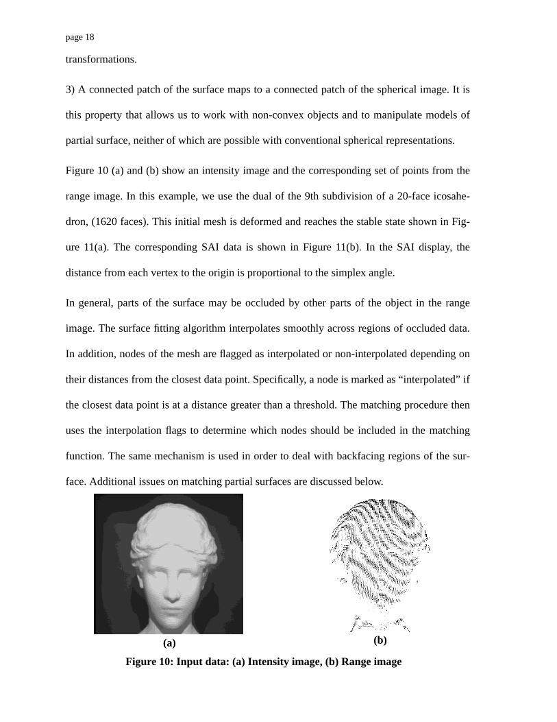
Figure 10 (a) and (b) show an intensity image and the corresponding set of points from the

range image. In this example, we use the dual of the 9th subdivision of a 20-face icosahe-

dron, (1620 faces). This initial mesh is deformed and reaches the stable state shown in Fig-

ure 11(a). The corresponding SAI data is shown in Figure 11(b). In the SAI display, the

distance from each vertex to the origin is proportional to the simplex angle.

In general, parts of the surface may be occluded by other parts of the object in the range

image. The surface fitting algorithm interpolates smoothly across regions of occluded data.

In addition, nodes of the mesh are flagged as interpolated or non-interpolated depending on

their distances from the closest data point. Specifically, a node is marked as “interpolated” if

the closest data point is at a distance greater than a threshold. The matching procedure then

uses the interpolation flags to determine which nodes should be included in the matching

function. The same mechanism is used in order to deal with backfacing regions of the sur-

face. Additional issues on matching partial surfaces are discussed below.

Figure 10: Input data: (a) Intensity image, (b) Range image

(a) (b)

which is sufficient for matching purposes. Finally, g(P) is invariant with respect to rotation,

translation, and scaling.

3.5. Deformable Surface Mapping

A regular mesh drawn on a closed surface can be mapped to a spherical mesh in a natural

way. For a given number of nodesK, we can associate with each node a unique index which

depends only on the topology of the mesh and which is independent of the shape of the

underlying surface. This numbering of the nodes defines a natural mappingh between any

meshM and a reference meshS on the unit sphere with the same number of nodes:h(P) is

the node ofS with the same index asP.

Given h, we can store at each nodeP of S the simplex angle of the corresponding node on

the surfaceg(h(P)). The resulting structure is a spherical image, that is, a tessellation on the

unit sphere, each node being associated with the simplex angle of a point on the original sur-

face. We call this representation the Spherical Attribute Image (SAI).

If the original meshM satisfies the local regularity constraint, then the corresponding SAI

has several invariance properties:

1) For a given number of nodes, the SAI is invariant by translation and scaling of the origi-

nal object.

2) The SAI represents an object unambiguously up to a rotation. More precisely, ifM andM’

are two tessellations of the same object with the same number of nodes, then the corre-

sponding SAIsS andS’ are identical up to a rotation of the unit sphere. One consequence of

this property is that two SAIs represent the same object if one is the rotated version of the

other. It is this property which will allow us to match surfaces that differ by arbitrary rigid

good approximation of the object surface. We need to add another constraint in order to

build meshes suitable for matching. Specifically, we need to make sure that the distribution

of mesh nodes on the surface is invariant with respect to rotation, translation and scale.

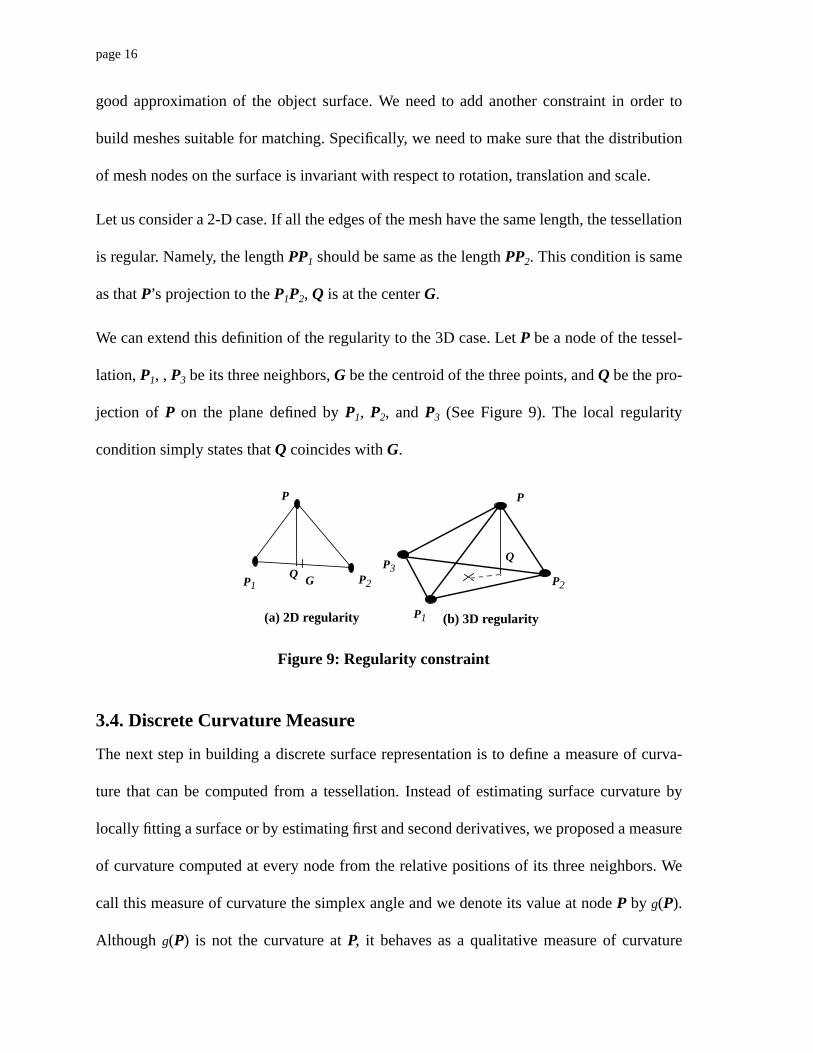
Let us consider a 2-D case. If all the edges of the mesh have the same length, the tessellation

is regular. Namely, the lengthPP1 should be same as the lengthPP2. This condition is same

as thatP’s projection to theP1P2, Q is at the centerG.

We can extend this definition of the regularity to the 3D case. LetP be a node of the tessel-

lation,P1, , P3 be its three neighbors,G be the centroid of the three points, andQ be the pro-

jection of P on the plane defined byP1, P2, andP3 (See Figure 9). The local regularity

condition simply states thatQ coincides withG.

3.4. Discrete Curvature Measure

The next step in building a discrete surface representation is to define a measure of curva-

ture that can be computed from a tessellation. Instead of estimating surface curvature by

locally fitting a surface or by estimating first and second derivatives, we proposed a measure

of curvature computed at every node from the relative positions of its three neighbors. We

call this measure of curvature the simplex angle and we denote its value at nodeP by g(P).

Although g(P) is not the curvature atP, it behaves as a qualitative measure of curvature

P1

P2

P3

P

Q

(b) 3D regularity(a) 2D regularity

P1 P2

P

QG

Figure 9: Regularity constraint

for many algorithms to have a constant number of neighbors at each node. We use a class of

tessellations such that each node has exactly three neighbors. Such a tessellation can be con-

structed as the dual of a triangulation of the surface.

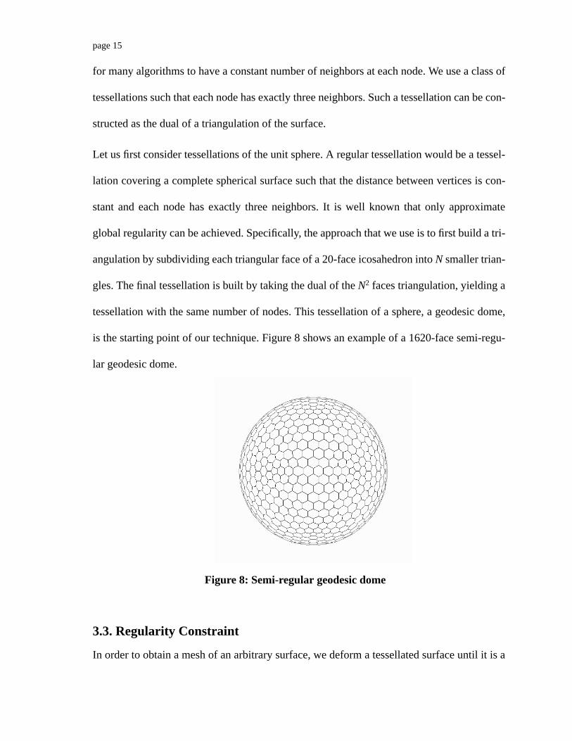
Let us first consider tessellations of the unit sphere. A regular tessellation would be a tessel-

lation covering a complete spherical surface such that the distance between vertices is con-

stant and each node has exactly three neighbors. It is well known that only approximate

global regularity can be achieved. Specifically, the approach that we use is to first build a tri-

angulation by subdividing each triangular face of a 20-face icosahedron intoN smaller trian-

gles. The final tessellation is built by taking the dual of theN2 faces triangulation, yielding a

tessellation with the same number of nodes. This tessellation of a sphere, a geodesic dome,

is the starting point of our technique. Figure 8 shows an example of a 1620-face semi-regu-

lar geodesic dome.

3.3. Regularity Constraint

In order to obtain a mesh of an arbitrary surface, we deform a tessellated surface until it is a

Figure 8: Semi-regular geodesic dome

invariants, Gaussian curvature is the most important. The distribution based on the Gaussian

curvature is referred to as the Spherical Attribute Image (SAI).

At each tessellation on the object surface, we calculate invariants such as Gaussian curva-

ture or surface albedo, and map them to the corresponding original tessellation of the geode-

sic dome. We can observe a distribution of invariants on the unit sphere. Among the possible

invariants, Gaussian curvature is the most important. The distribution based on the Gaussian

curvature is referred to as the Spherical Attribute Image (SAI).

In the following section, we will briefly describe the SAI. First, we explain how to tessellate

an arbitrary surface into a semi-regular mesh, and how to calculate the simplex angle (dis-

cretized Gaussian curvature), a variation of curvature, at the nodes of the mesh, and how to

map the mesh to a spherical image. Finally, we discuss how to handle partial views of 3-D

objects.

3.2. Semi-Regular Tessellation

A natural discrete representation of a surface is a graph of points, or tessellation, such that

each node is connected to each of its closest neighbor by an arc of the graph. It is desirable

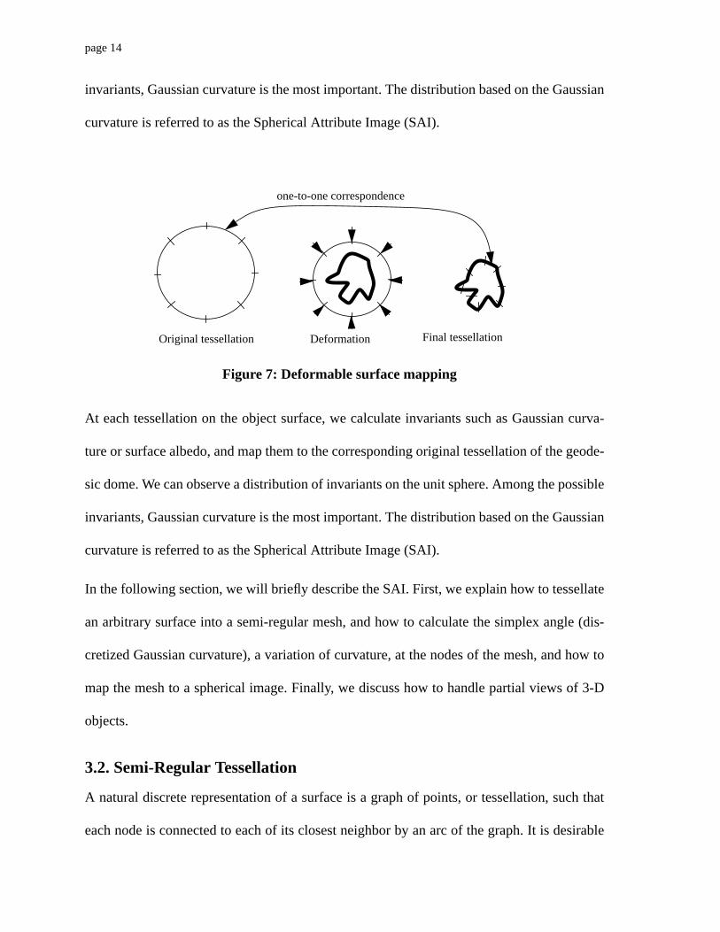
Original tessellation Deformation Final tessellation

one-to-one correspondence

Figure 7: Deformable surface mapping

3. Spherical Attribute Image

3.1. A Novel Mapping Based On Deformable Surface

The fundamental problem of the EGI family is that it depends on the Gauss mapping. For

that reason, more than two parts on an object surface may be mapped on the same point of

the sphere. More than two objects may have the same EGI. Further, a partial EGI from a part

of an object is not same as a part of EGI from the whole object. Thus, under occlusion, we

cannot perform the EGI matching. This problem is due to the fact that the Gauss mapping is

not unique for non-convex objects.

We have derived a novel method to make a one-to-one mapping between a non-convex

object surface and a spherical surface [11,13]. The method uses a deformable surface. We

first prepare a semi-regularly tessellated geodesic dome (a tessellated unit sphere). Then, we

deform the geodesic dome onto an object surface as close as possible (data force) while

maintaining the local regularity constraint (regularization force): to ensure that tessellations

have a similar area and the same topology as one another. The final representation is given

as the equilibrium between the data force and the regularization force. By doing so, 1) the

object surface is semi-uniformly tessellated, 2) each tessellation on the object surface has a

counterpart on the undeformed geodesic dome (unit sphere); thus, we can establish a one-to-

one mapping between the object surface and the unit sphere. The mapping is referred to as

deformable surface mapping (DSP) (see Figure 7).

At each tessellation on the object surface, we calculate invariants such as Gaussian curva-

ture or surface albedo, and map them to the corresponding original tessellation of the geode-

sic dome. We can observe a distribution of invariants on the unit sphere. Among the possible

tion is the signed distance of the oriented tangent plane from a predefined origin. He pro-

poses to ascribe to each different surface a separate support function value. This means that,

in general, the proposed variant of the Gauss map of a surface is not globally one to one.

Although it is less compact it can uniquely determine a surface. A method to determine

object pose based on this representation was not presented in Nalwa’s paper.

Roach et al. [10] encode positional information by expressing the equation of a surface

patch in dual space. The resulting encoded representation is called the spherical dual image.

A point in the dual space represents both the orientation and position of a patch; edges are

explicitly described as connections between dual points. A drawback of this approach is that

planes passing near or through the designated origin cannot be dualized properly; they map

to infinity or very large values.

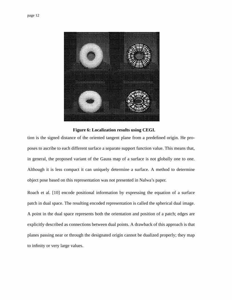
Figure 6: Localization results using CEGI.

Hence, for each point of the CEGI, the magnitude of the weight is independent of the trans-

lation. The complex number wraps around for every translation distance of 2π. Therefore,

the computed translation is known only up to 2π. To eliminate this ambiguity, all distances

are normalized such that the greatest expected change in translation distance isπ.

2.3.2. Pose Determination StrategyGiven a prototype CEGI and a partial CEGI of an unknown object, we can recognize the

object and determine its orientation as follows: First, we calculate the magnitude distribu-

tions of both CEGI’s, and second, we match the resulting distribution with that of the proto-

type. Once both the object and its orientation with respect to the stored model are identified,

the object translation can be calculated by using the suitably oriented CEGI’s.

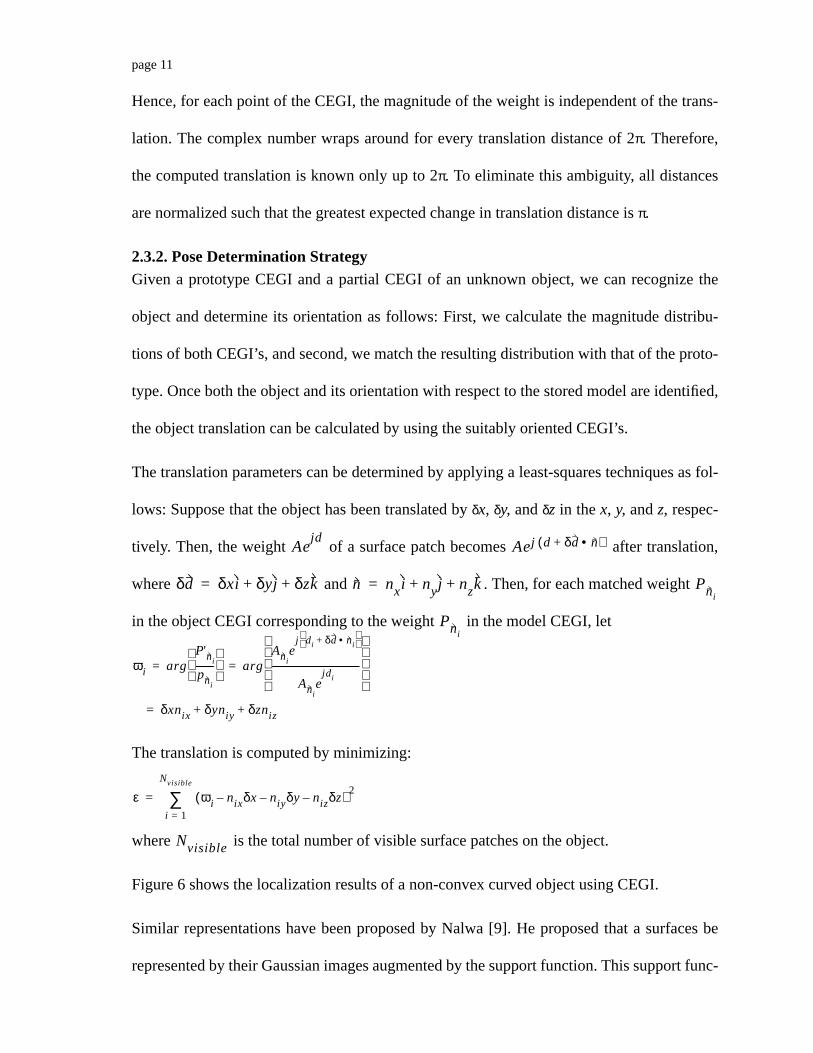
The translation parameters can be determined by applying a least-squares techniques as fol-

lows: Suppose that the object has been translated byδx, δy, andδz in thex, y, and z, respec-

tively. Then, the weight of a surface patch becomes after translation,

where and . Then, for each matched weight

in the object CEGI corresponding to the weight in the model CEGI, let

The translation is computed by minimizing:

where is the total number of visible surface patches on the object.

Figure 6 shows the localization results of a non-convex curved object using CEGI.

Similar representations have been proposed by Nalwa [9]. He proposed that a surfaces be

represented by their Gaussian images augmented by the support function. This support func-

Aejd

Aej d δd n•+( )

δd δxi δyj δzk+ += n nxi nyj nzk+ += Pni

Pni

ωi argP'ni

pni

--------

argAni

ej di δd ni•+

Anie

jdi---------------------------------------

= =

δxnix δyniy δzniz+ +=

ε ωi nixδx– niyδy– nizδz–( ) 2

i 1=

Nvisible

∑=

Nvisible

For any given point in the CEGI corresponding to normal , the magnitude of the point’s

weight is .A is independent of the normal distance, and if the object is convex, the dis-

tribution of A corresponds to the conventional EGI representation. If the object is not con-

vex, the magnitude of each weight will not necessarily be equal to the weight in the

corresponding conventional EGI.

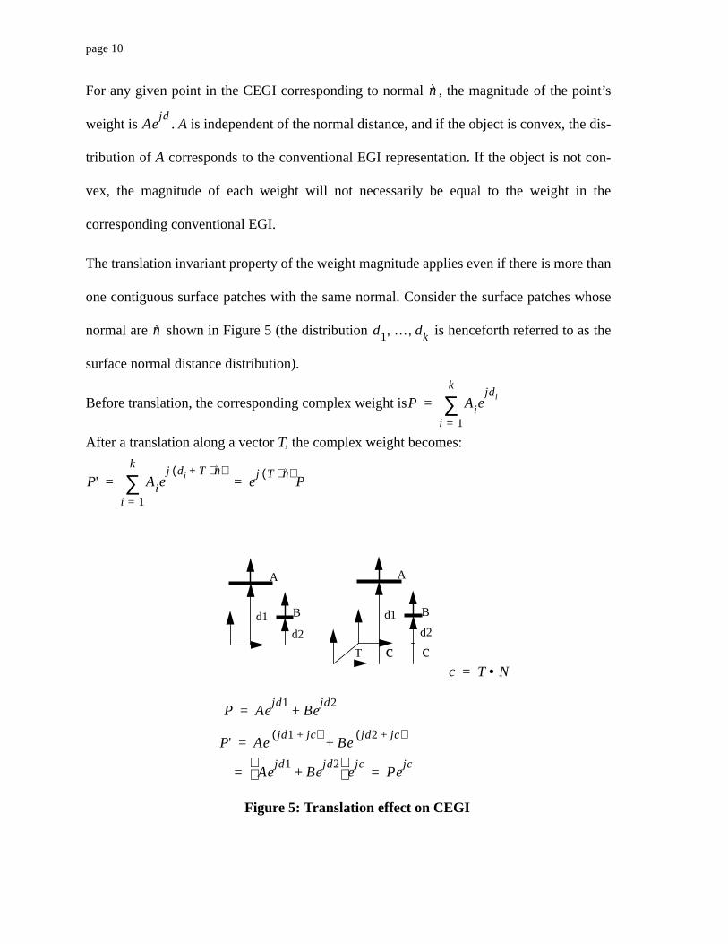
The translation invariant property of the weight magnitude applies even if there is more than

one contiguous surface patches with the same normal. Consider the surface patches whose

normal are shown in Figure 5 (the distribution is henceforth referred to as the

surface normal distance distribution).

Before translation, the corresponding complex weight is

After a translation along a vectorT, the complex weight becomes:

n

Aejd

n d1 … dk, ,

P Aiejdl

i 1=

k

∑=

P' Aiej di T n⋅+( )

i 1=

k

∑ ej T n⋅( )

P= =

A

Bd1

d2

A

Bd1

d2

c cT

c T N•=

P Aejd1

Bejd2

+=

P' Aejd1 jc+( )

Bejd2 jc+( )

+=

Aejd1

Bejd2

+

ejc

Pejc

= =

Figure 5: Translation effect on CEGI

2.3. Complex EGI

2.3.1. DefinitionOne of the problems with the EGI is that we can determine the rotation of an object but can-

not determine the translation of the object. In order to recover translation, we have intro-

duced the complex EGI to encode positional information.

We will assume some arbitrary origin of an object. We will measure the distance,d, from

this origin to each surface patch. We will stored at the corresponding point of the Gaussian

sphere. The CEGI weight at each point on the Gaussian sphere is a complex number whose

magnitude is the surface area and whose phase is the distance information. When an object

translates, the magnitude of the complex mass remains the same while its phase changes

accordingly.

Object recognition is accomplished by EGI matching using the magnitude only. The transla-

tion component is computed by using the phase difference.

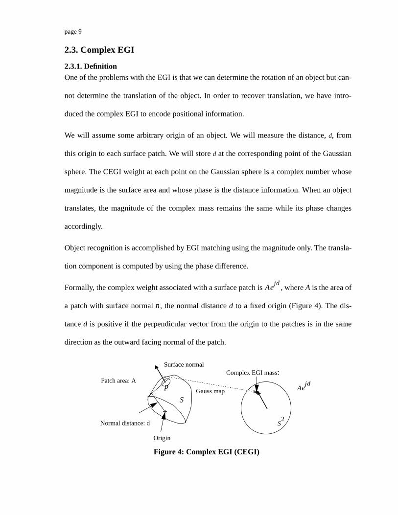
Formally, the complex weight associated with a surface patch is , whereA is the area of

a patch with surface normal , the normal distanced to a fixed origin (Figure 4). The dis-

tanced is positive if the perpendicular vector from the origin to the patches is in the same

direction as the outward facing normal of the patch.

Aejd

n

S2

p

SGauss map

Origin

Normal distance: d

Surface normal

Patch area: AComplex EGI mass:

Aejd

Figure 4: Complex EGI (CEGI)

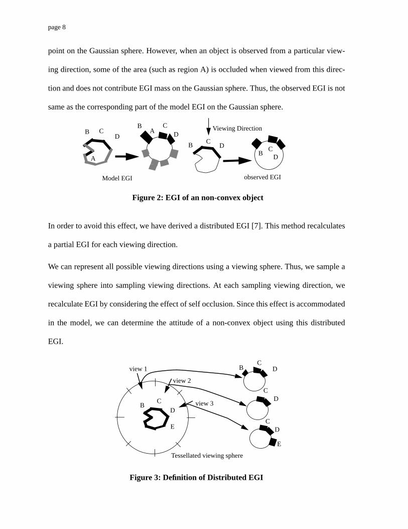
point on the Gaussian sphere. However, when an object is observed from a particular view-

ing direction, some of the area (such as region A) is occluded when viewed from this direc-

tion and does not contribute EGI mass on the Gaussian sphere. Thus, the observed EGI is not

same as the corresponding part of the model EGI on the Gaussian sphere.

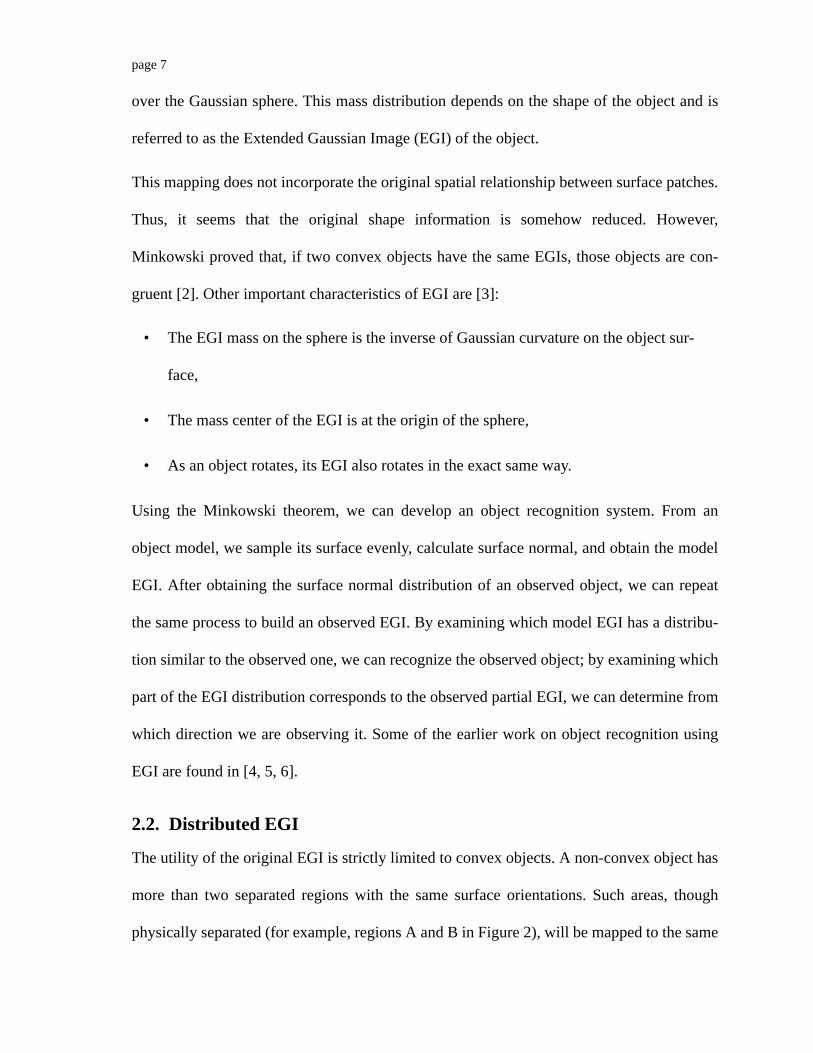
In order to avoid this effect, we have derived a distributed EGI [7]. This method recalculates

a partial EGI for each viewing direction.

We can represent all possible viewing directions using a viewing sphere. Thus, we sample a

viewing sphere into sampling viewing directions. At each sampling viewing direction, we

recalculate EGI by considering the effect of self occlusion. Since this effect is accommodated

in the model, we can determine the attitude of a non-convex object using this distributed

EGI.

A

B CD

AB C

D

BC

DB

CD

Model EGI observed EGI

Viewing Direction

Figure 2: EGI of an non-convex object

BC

D

BC

D

Tessellated viewing sphere

CD

CDE

E

view 1

view 2

view 3

Figure 3: Definition of Distributed EGI

over the Gaussian sphere. This mass distribution depends on the shape of the object and is

referred to as the Extended Gaussian Image (EGI) of the object.

This mapping does not incorporate the original spatial relationship between surface patches.

Thus, it seems that the original shape information is somehow reduced. However,

Minkowski proved that, if two convex objects have the same EGIs, those objects are con-

gruent [2]. Other important characteristics of EGI are [3]:

• The EGI mass on the sphere is the inverse of Gaussian curvature on the object sur-

face,

• The mass center of the EGI is at the origin of the sphere,

• As an object rotates, its EGI also rotates in the exact same way.

Using the Minkowski theorem, we can develop an object recognition system. From an

object model, we sample its surface evenly, calculate surface normal, and obtain the model

EGI. After obtaining the surface normal distribution of an observed object, we can repeat

the same process to build an observed EGI. By examining which model EGI has a distribu-

tion similar to the observed one, we can recognize the observed object; by examining which

part of the EGI distribution corresponds to the observed partial EGI, we can determine from

which direction we are observing it. Some of the earlier work on object recognition using

EGI are found in [4, 5, 6].

2.2. Distributed EGI

The utility of the original EGI is strictly limited to convex objects. A non-convex object has

more than two separated regions with the same surface orientations. Such areas, though

physically separated (for example, regions A and B in Figure 2), will be mapped to the same

2. Gauss Mapping and Related Representations

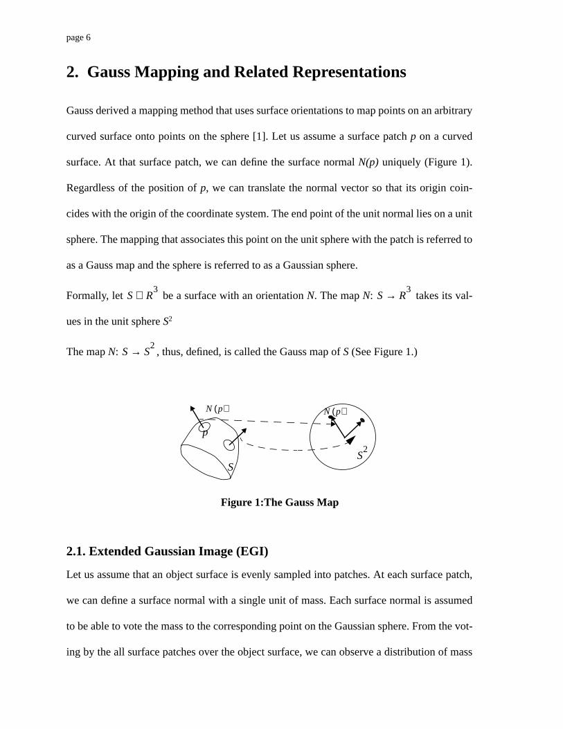
Gauss derived a mapping method that uses surface orientations to map points on an arbitrary

curved surface onto points on the sphere [1]. Let us assume a surface patchp on a curved

surface. At that surface patch, we can define the surface normalN(p) uniquely (Figure 1).

Regardless of the position ofp, we can translate the normal vector so that its origin coin-

cides with the origin of the coordinate system. The end point of the unit normal lies on a unit

sphere. The mapping that associates this point on the unit sphere with the patch is referred to

as a Gauss map and the sphere is referred to as a Gaussian sphere.

Formally, let be a surface with an orientationN. The mapN: takes its val-

ues in the unit sphereS2

The mapN: , thus, defined, is called the Gauss map ofS (See Figure 1.)

2.1. Extended Gaussian Image (EGI)

Let us assume that an object surface is evenly sampled into patches. At each surface patch,

we can define a surface normal with a single unit of mass. Each surface normal is assumed

to be able to vote the mass to the corresponding point on the Gaussian sphere. From the vot-

ing by the all surface patches over the object surface, we can observe a distribution of mass

S R3⊂ S R

3→

S S2→

Figure 1:The Gauss Map

S2

N p( )

p

N p( )

S

surface do carry useful information, such as curvature, for recognition.

It is desirable to assign a coordinate system to curved surfaces and to use invariant features,

including curvature distributions, along this particular coordinate system. This coordinate

system should be independent of the viewing direction. Since it is difficult to reliably seg-

ment a curved surface into regions, it is also desirable to define a coordinate system over the

entire object surface.

Aspherical representation maps an entire object surface to a standard coordinate system (a

unit sphere). Objects usually handled by vision systems have closed surfaces: topologically

equivalent to a spherical surface. Thus, we began our effort to develop a mapping method

from an arbitrary object surface to a spherical surface and store invariants over the spherical

surface. It is possible to define a coordinate system on a surface using two parameters such

as longitude and latitude. Such parametrization, however, require specific information, that

is, the direction of an imaginary line between North and South poles.

This paper briefly overviews our earlier efforts on such spherical representations. We begin

with a discussion of the Extended Gaussian Image developed around 1980, and, continue on

to describe our recent work on the Spherical Attribute Image.

1. Introduction

One of the fundamental problems in object recognition is how to represent the objects mod-

els. The representation govern the characteristics and efficiencies of recognition systems.

We restrict ourselves here to surface-based representations since those are the most relevant

in computer vision.

A surface-based representation describes an object as a collection of visible “faces” of the

object. Since imaging systems provide the same information as surface-based representa-

tions, it is relatively easy to use surface-based representation for object recognition. Repre-

sentative surface-based representations include edge-and/or face-based invariants, aspect

graphs, and spherical representations.

The simplest type of object representation is based on planar faces. A planar face has a clear

boundary of surface orientation discontinuity and its internal pixels provide less informa-

tion. A polyhedron, consisting of planar faces, effectively represents the relations between

faces for recognition. Early works by Oshima-Shirai [14] and Bolles [15] effectively use

such graphs of visible face relations.

One of the basic problems in using such visible graphs was determining the number of dif-

ferent graphs required to represent one object. Koendering’s aspect answers this question

[16]. The aspect representation specifies an object as a collection of all possible topologi-

cally different relational graphs of visible faces. Our earlier work on the vision algorithm

compiler used this aspect representation for object recognition.

For curved object recognition, the boundary of a curved surface patch is often ill-defined;

the relative relationships between faces are unreliable. Fortunately, however, points on the

Abstract

One of the fundamental problems in representing a curved surface is how to

define an intrinsic, i.e., viewer independent, coordinate system over a curved

object surface. In order to establish point matching between model and observed

feature distributions over the standard coordinate system, we need to set up a

coordinate system that maps a point on a curved surface to a point on a standard

coordinate system. This mapping should be independent of the viewing direc-

tion. Since the boundary of a 3-D object forms a closed surface, a coordinate sys-

tem defined on the sphere is preferred.

We have been exploring several intrinsic mappings from an object surface to a

spherical surface. We have investigated several representations including: the

EGI (Extended Gaussian Image), the DEGI (Distributed Extended Gaussian

Image), the CEGI (Complex Extended Gaussian Image), and the SAI (Spherical

Attribute Image). This paper summarizes our motivations to derive each repre-

sentation and the lessons that we have learned through this endeavor.

Keywords: Computer Vision, Scene Understanding, Robotics, Object Representation, GaussMap, Gaussian Sphere, Differential Geometry

School of Computer ScienceCarnegie Mellon University

Pittsburgh, Pennsylvania 15213-3890

Spherical Representations: from EGI to SAI

Katsushi Ikeuchi and Martial Hebert

October 1995CMU-CS-95-197

The research is sponsored in part by the Advanced Research Projects Agency under the ArmyResearch Office under Grant DAAH04-94-G-0006, and in part by National Science Foundationunder Grant IRI-9224521.

The views and conclusions contained in this document are those of the authors, and should not beinterpreted as representing the official policies, either expressed or implied, of NSF, ARPA, or theU.S. government.

IEEE Trans. Pattern Analysis and Machine Intelligence 1983 ...

Documents

Transcript of IEEE Trans. Pattern Analysis and Machine Intelligence 1983 ...