IEEE TRANS. AUDIO, SPEECH, AND LANGUAGE … · as voice search and voice interaction with mobile...
33
IEEE TRANS. AUDIO, SPEECH, AND LANGUAGE PROCESSING, VOL. X, NO. X, XXX 2013 1 An Overview of Noise-Robust Automatic Speech Recognition Jinyu Li, Member, IEEE, Li Deng, Fellow, IEEE, Yifan Gong, Senior Member, IEEE, and Reinhold Haeb-Umbach, Senior Member, IEEE Abstract—New waves of consumer-centric applications, such as voice search and voice interaction with mobile devices and home entertainment systems, increasingly require automatic speech recognition (ASR) to be robust to the full range of real- world noise and other acoustic distorting conditions. Despite its practical importance, however, the inherent links between and distinctions among the myriad of methods for noise-robust ASR have yet to be carefully studied in order to advance the field further. To this end, it is critical to establish a solid, consistent, and common mathematical foundation for noise-robust ASR, which is lacking at present. This article is intended to fill this gap and to provide a thorough overview of modern noise-robust techniques for ASR developed over the past 30 years. We emphasize methods that are proven to be successful and that are likely to sustain or expand their future applicability. We distill key insights from our comprehensive overview in this field and take a fresh look at a few old problems, which nevertheless are still highly relevant today. Specifically, we have analyzed and categorized a wide range of noise-robust techniques using five different criteria: 1) feature-domain vs. model-domain processing, 2) the use of prior knowledge about the acoustic environment distortion, 3) the use of explicit environment-distortion models, 4) deterministic vs. uncertainty processing, and 5) the use of acoustic models trained jointly with the same feature enhancement or model adaptation process used in the testing stage. With this taxonomy- oriented review, we equip the reader with the insight to choose among techniques and with the awareness of the performance- complexity tradeoffs. The pros and cons of using different noise- robust ASR techniques in practical application scenarios are provided as a guide to interested practitioners. The current challenges and future research directions in this field is also carefully analyzed. I. I NTRODUCTION Automatic speech recognition (ASR) is the process and the related technology for converting the speech signal into its corresponding sequence of words or other linguistic entities by means of algorithms implemented in a device, a computer, or computer clusters [1], [2]. Historically, ASR applications have included voice dialing, call routing, interactive voice response, data entry and dictation, voice command and con- trol, structured document creation (e.g., medical and legal transcriptions), appliance control by voice, computer-aided language learning, content-based spoken audio search, and robotics. More recently, with the exponential growth of big data and computing power, ASR technology has advanced to the stage where more challenging applications are becoming Dr. Jinyu Li, Dr. Li Deng, and Dr. Yifan Gong are with Microsoft Corpo- ration, Redmond, WA, U.S.; Dr. Reinhold Haeb-Umbach is with University of Paderborn, Paderborn, Germany a reality. Examples are voice search and interactions with mobile devices (e.g., Siri on iPhone, Bing voice search on win- Phone, and Google Now on Andriod), voice control in home entertainment systems (e.g., Kinect on xBox), and various speech-centric information processing applications capitalizing on downstream processing of ASR outputs [3]. For such large- scale, real-world applications, noise robustness is becoming an increasingly important core technology since ASR needs to work in much more difficult acoustic environments than in the past [4]. A large number of noise-robust ASR methods, in the order of hundreds, have been proposed and published over the past 30 years or so, and many of them have created significant im- pact on either research or commercial use. Such accumulated knowledge deserves thorough examination not only to define the state of the art in this field from a fresh and unifying perspective but also to point to fruitful future directions in the field. Nevertheless, a well-organized framework for relating and analyzing these methods is conspicuously missing. The existing survey papers [5]–[13] in noise-robust ASR either do not cover all recent advances in the field or focus only on a specific sub-area. Although there are also few recent books [14], [15], they are collections of topics with each chapter written by different authors and it is hard to provide a unified view across all topics. Given the importance of noise-robust ASR, the time is ripe to analyze and unify the solutions. In this paper, we elaborate on the basic concepts in noise-robust ASR and develop categorization criteria and unifying themes. Specifically, we hierarchically classify the major and significant noise-robust ASR methods using a con- sistent and unifying mathematical language. We establish their interrelations and differentiate among important techniques, and discuss current technical challenges and future research directions. This paper also identifies relatively promising, short-term new research areas based on a careful analysis of successful methods, which can serve as a reference for future algorithm development in the field. Furthermore, in the literature spanning over 30 years on noise-robust ASR, there is inconsistent use of basic concepts and terminology as adopted by different researchers in the field. This kind of inconsistency sometimes brings confusion to the field, especially for new researchers and students. It is therefore important to examine discrepancies in the current literature and re-define consistent terminology, another goal of this overview paper. This paper is organized as follows. In Section II, we discuss the fundamentals of noise-robust ASR. The impact of noise and channel distortions on clean speech is examined. Then,
Transcript of IEEE TRANS. AUDIO, SPEECH, AND LANGUAGE … · as voice search and voice interaction with mobile...
IEEE TRANS. AUDIO, SPEECH, AND LANGUAGE PROCESSING, VOL. X, NO. X, XXX 2013 1
An Overview of Noise-Robust Automatic SpeechRecognition
Jinyu Li, Member, IEEE, Li Deng, Fellow, IEEE, Yifan Gong, Senior Member, IEEE, and ReinholdHaeb-Umbach, Senior Member, IEEE
Abstract—New waves of consumer-centric applications, suchas voice search and voice interaction with mobile devices andhome entertainment systems, increasingly require automaticspeech recognition (ASR) to be robust to the full range of real-world noise and other acoustic distorting conditions. Despite itspractical importance, however, the inherent links between anddistinctions among the myriad of methods for noise-robust ASRhave yet to be carefully studied in order to advance the fieldfurther. To this end, it is critical to establish a solid, consistent,and common mathematical foundation for noise-robust ASR,which is lacking at present.
This article is intended to fill this gap and to provide athorough overview of modern noise-robust techniques for ASRdeveloped over the past 30 years. We emphasize methods thatare proven to be successful and that are likely to sustain orexpand their future applicability. We distill key insights fromour comprehensive overview in this field and take a fresh look ata few old problems, which nevertheless are still highly relevanttoday. Specifically, we have analyzed and categorized a widerange of noise-robust techniques using five different criteria:1) feature-domain vs. model-domain processing, 2) the use ofprior knowledge about the acoustic environment distortion, 3)the use of explicit environment-distortion models, 4) deterministicvs. uncertainty processing, and 5) the use of acoustic modelstrained jointly with the same feature enhancement or modeladaptation process used in the testing stage. With this taxonomy-oriented review, we equip the reader with the insight to chooseamong techniques and with the awareness of the performance-complexity tradeoffs. The pros and cons of using different noise-robust ASR techniques in practical application scenarios areprovided as a guide to interested practitioners. The currentchallenges and future research directions in this field is alsocarefully analyzed.
I. INTRODUCTION
Automatic speech recognition (ASR) is the process and therelated technology for converting the speech signal into itscorresponding sequence of words or other linguistic entitiesby means of algorithms implemented in a device, a computer,or computer clusters [1], [2]. Historically, ASR applicationshave included voice dialing, call routing, interactive voiceresponse, data entry and dictation, voice command and con-trol, structured document creation (e.g., medical and legaltranscriptions), appliance control by voice, computer-aidedlanguage learning, content-based spoken audio search, androbotics. More recently, with the exponential growth of bigdata and computing power, ASR technology has advanced tothe stage where more challenging applications are becoming
Dr. Jinyu Li, Dr. Li Deng, and Dr. Yifan Gong are with Microsoft Corpo-ration, Redmond, WA, U.S.; Dr. Reinhold Haeb-Umbach is with Universityof Paderborn, Paderborn, Germany
a reality. Examples are voice search and interactions withmobile devices (e.g., Siri on iPhone, Bing voice search on win-Phone, and Google Now on Andriod), voice control in homeentertainment systems (e.g., Kinect on xBox), and variousspeech-centric information processing applications capitalizingon downstream processing of ASR outputs [3]. For such large-scale, real-world applications, noise robustness is becomingan increasingly important core technology since ASR needsto work in much more difficult acoustic environments than inthe past [4].
A large number of noise-robust ASR methods, in the orderof hundreds, have been proposed and published over the past30 years or so, and many of them have created significant im-pact on either research or commercial use. Such accumulatedknowledge deserves thorough examination not only to definethe state of the art in this field from a fresh and unifyingperspective but also to point to fruitful future directions in thefield. Nevertheless, a well-organized framework for relatingand analyzing these methods is conspicuously missing. Theexisting survey papers [5]–[13] in noise-robust ASR eitherdo not cover all recent advances in the field or focus onlyon a specific sub-area. Although there are also few recentbooks [14], [15], they are collections of topics with eachchapter written by different authors and it is hard to providea unified view across all topics. Given the importance ofnoise-robust ASR, the time is ripe to analyze and unify thesolutions. In this paper, we elaborate on the basic conceptsin noise-robust ASR and develop categorization criteria andunifying themes. Specifically, we hierarchically classify themajor and significant noise-robust ASR methods using a con-sistent and unifying mathematical language. We establish theirinterrelations and differentiate among important techniques,and discuss current technical challenges and future researchdirections. This paper also identifies relatively promising,short-term new research areas based on a careful analysisof successful methods, which can serve as a reference forfuture algorithm development in the field. Furthermore, in theliterature spanning over 30 years on noise-robust ASR, there isinconsistent use of basic concepts and terminology as adoptedby different researchers in the field. This kind of inconsistencysometimes brings confusion to the field, especially for newresearchers and students. It is therefore important to examinediscrepancies in the current literature and re-define consistentterminology, another goal of this overview paper.
This paper is organized as follows. In Section II, we discussthe fundamentals of noise-robust ASR. The impact of noiseand channel distortions on clean speech is examined. Then,
2 IEEE TRANS. AUDIO, SPEECH, AND LANGUAGE PROCESSING, VOL. X, NO. X, XXX 2013
we build a general framework for noise-robust ASR and definefive ways of categorizing noise-robust ASR techniques. (Thisexpands the previous taxonomy-oriented review from the useof two criteria to five [10].) Section III is devoted to the firstcategory — feature-domain vs. model-domain techniques. Thesecond category, detailed in Section IV, comprises methodsthat exploit prior knowledge about the signal distortion. Meth-ods that incorporate an explicit distortion model to predict thedistorted speech from a clean one define the third category,covered in Section V. The use of uncertainty constitutes thefourth way to categorize a wide range of noise-robust ASRalgorithms, and is covered in Section VI. Uncertainty in eitherthe model space or feature space may be incorporated withinthe Bayesian framework to promote noise-robust ASR. Thefinal, fifth way to categorize and analyze noise-robust ASRtechniques utilizes joint model training, described in SectionVII. With joint model training, environmental variability inthe training data is removed in order to generate canonicalmodels. We conclude this overview paper in Section VIII, withdiscussions on future directions for noise-robust ASR.
II. THE BACKGROUND AND SCOPE
In this section, we establish some fundamental conceptsthat are most relevant to the discussions in the remainder ofthis paper. Since mathematical language is an essential toolin our exposition, we first introduce our notation in Table I.Throughout this paper, vectors are in bold type and matricesare capitalized.
TABLE IDEFINITIONS OF A SUBSET OF COMMONLY USED SYMBOLS AND NOTIONS
IN THIS ARTICLE
Symbol MeaningT number of frames in a speech sequenceX sequence of clean speech vectors (x1,x2, ......,xT )
Y sequence of distorted speech vectors (y1,y2, ......,yT )
θ sequence of speech states (θ1, θ2, ......, θT )
Λ acoustic model parameterΓ language model parameterC discrete cosine transform (DCT) matrixx clean speech in the cepstral domainy distorted speech in the cepstral domainn noise in the cepstral domainh channel in the cepstral domainµx clean speech mean in the cepstral domainµy distorted speech mean in the cepstral domainµn noise mean in the cepstral domainµh channel mean in the cepstral domainN Gaussian distribution
A. Modeling Distortions of Speech in Acoustic Environments
Mel-frequency cepstral coefficients (MFCCs) [16] are themost widely used acoustic features. The short-time discreteFourier transform (STDFT) is applied to the speech signal,and the power or magnitude spectrum is generated. A set ofMel scale filters is applied to obtain Mel-filter-bank output.
Then the log operator is used to get the log-filter-bank output.Finally, the discrete cosine transform (DCT) is used to generateMFCCs. In the following, we use MFCCs as the acousticfeature to elaborate on the relation between clean and distortedspeech.
Figure 1 shows a time domain model for speech degradedby both additive noise and convolutive channel distortions [5].The observed distorted speech signal y[m], where m denotesthe discrete time index, is generated from the clean speechsignal x[m] with additive noise n[m] and convolutive channeldistortions h[m] according to
y[m] = x[m] ∗ h[m] + n[m], (1)
where ’∗’ denotes the convolution operator.
Fig. 1. A model of acoustic environment distortion in the discrete-timedomain relating clean speech samples x[m] to distorted speech samples y[m].
After applying the STDFT, the following equivalent relationcan be established in the spectral domain:
y[k] = x[k]h[k] + n[k]. (2)
Here, k is the frequency bin index. Note that we left out theframe index for ease of notation. To arrive at Eq-2 we assumedthat the impulse response h[m] is much shorter than the DFTanalysis window. Then we can make use of the multiplicativetransfer function approximation by which a convolution in thetime domain corresponds to a multiplication in the STDFTdomain [17]. This approximation does not hold in the presenceof reverberated speech, because the acoustic impulse responsecharacterizing the reverberation is typically much longer thanthe STDFT window size. Thus Eq-2 is not adequate to describereverberated speech in the STDFT domain.
The power spectrum of the distorted speech can then beobtained as:
|y[k]|2 = |x[k]|2|h[k]|2 + |n[k]|2 + 2|x[k]||h[k]||n[k]| cosβk,(3)
where βk denotes the (random) angle between the two com-plex variables n[k] and x[k]h[k]. If cosβk is set as 0, Eq-3will become:
|y[k]|2 = |x[k]|2|h[k]|2 + |n[k]|2. (4)
Removing this “phase” term is a common practice in theformulation of speech distortion in the power spectral domain;e.g. in the spectral subtraction technique. So is approximatingthe phase term in the log-spectral domain; e.g. [18]. Whileachieving simplicity in developing speech enhancement algo-rithms, removing this term is a partial cause of the degradationof enhancement performance at low SNRs (around 0 dB) [19].
By applying a set of Mel-scale filters (L in total) to thepower spectrum in Eq-3, we have the l-th Mel-filter-bank
J. LI et al.: AN OVERVIEW OF NOISE-ROBUST AUTOMATIC SPEECH RECOGNITION 3
energies for distorted speech, clean speech, noise and channel:
|y[l]|2 =∑k
Wk[l]|y[k]|2 (5)
|x[l]|2 =∑k
Wk[l]|x[k]|2 (6)
|n[l]|2 =∑k
Wk[l]|n[k]|2 (7)
|h[l]|2 =
∑kWk[l]|x[k]|2|h[k]|2
|x[l]|2(8)
where the l-th filter is characterized by the transfer functionWk[l] ≥ 0 with
∑kWk[l] = 1.
The phase factor α[l] of the l-th Mel-filter-bank is [19]
α[l] =
∑kWk[l]|x[k]||h[k]||n[k]| cosβk
|x[l]||h[l]||n[l]|(9)
Then, the following relation is obtained in the Mel-filter-bankdomain for the l-th Mel-filter-bank output
|y[l]|2 = |x[l]|2|h[l]|2 + |n[l]|2 + 2α[l]|x[l]||h[l]||n[l]|, (10)
By taking the log operation in both sides of Eq-10, we havethe following in the log-Mel-filter-bank domain, using vectornotation
y = x + h + log(
1 + exp(n− x− h)
+2α. ∗ exp(n− x− h
2)
). (11)
The .∗ operation for two vectors denotes element-wise product,and taking the logarithm and exponentiation of a vector aboveare also element-wise operations.
By applying the DCT transform to Eq-11, we can get thedistortion formulation in the cepstral domain as
y = x + h + C log(1 + exp(C−1(n− x− h))
+2α. ∗ exp(C−1 n− x− h
2)
), (12)
where C denotes the DCT matrix.In [19], it was shown that the phase factor α[l] for each Mel-
filter l can be approximated by a weighted sum of a numberof independent zero-mean random variables distributed over[−1, 1], where the total number of terms equals the numberof DFT bins. When the number of terms becomes large, thecentral limit theorem postulates that α[l] will be approximatelyGaussian. A more precise statistical description has beendeveloped in [20], where it is shown that all moments of α[l]of odd order are zero.
If we ignore the phase factor, Eq-11 and Eq-12 can besimplified to
y = x + h + log(1 + exp(n− x− h)), (13)y = x + h + C log(1 + exp(C−1(n− x− h))), (14)
which are the log-Mel-filter-bank and cepstral representations,respectively, corresponding to Eq-4 in the power spectraldomain. Eq-13 and Eq-14 are widely used in noise-robustASR technology as the basic formulation that characterizes
the relationship between clean and distorted speech in thelogarithmic domain. The effect of the phase factor is smallif noise estimates are poor. However, with an increase in thequality of the noise estimates, the effect of the phase factor isshown experimentally to be stronger [19].
In ASR, Gaussian mixture models (GMMs) are widely usedto characterize the distribution of speech in the log-Mel-filter-bank or cepstral domain. It is important to understand theimpact of noise, which is additive in the spectral domain,on the distribution of noisy speech in the log-Mel-filter-bankand cepstral domains. Using Eq-13 while setting h = 0 forsimplicity, we can simulate noisy speech in the log-filter-bankdomain. In Figure 2, we show the impact of noise on the cleanspeech signal in the log-filter-bank domain with increasingnoise mean values, i.e., decreasing SNRs. The clean speechshown with solid lines is Gaussian distributed, with a meanvalue of 25 and a standard deviation of 10. The noise n is alsoGaussian distributed, with different mean values and a standarddeviation of 2. The noisy speech shown with dashed linesdeviates from the Gaussian distribution to a varying degree.We can use a Gaussian distribution, shown with dotted lines,to make an approximation. The approximation error is largein the low SNR cases. When the noise mean is raised to 20and 25, as in Figure 2(c) and 2(d), the distribution of noisyspeech is skewed far away from a Gaussian distribution.
A natural way to deal with noise in the acoustic environmentis to use multi-style training [21], which trains the acousticmodel with all available noisy speech data. The hope is thatone of the noise types in the training set will appear in thedeployment scenario. However, there are two major problemswith multi-style training. The first is that during training it ishard to enumerate all noise types and SNRs encountered in testenvironments. The second is that the model trained with multi-style training has a very broad distribution because it needs tomodel all the environments. Given the unsatisfactory behaviorof multi-style training, it is necessary to work on technologiesthat directly deal with the noise and channel impacts. In thenext section, we lay down a general mathematical frameworkfor noise-robust speech recognition.
B. A General Framework for Noise-Robust Speech Recogni-tion
The goal of ASR is to obtain the optimal word sequence W,given the spoken speech signal X, which can be formulatedas the well-known maximum a posteriori (MAP) problem:
W = argmaxW
PΛ,Γ(W|X), (15)
where Λ and Γ are the acoustic model (AM) and languagemodel (LM) parameters. Using Bayes’ rule
PΛ,Γ(W|X) =pΛ(X|W)PΓ(W)
p(X), (16)
Eq-15 can be re-written as:
W = argmaxW
pΛ(X|W)PΓ(W), (17)
where pΛ(X|W) is the AM likelihood and PΓ(W) is theLM probability. When the time sequence is expanded and the

4 IEEE TRANS. AUDIO, SPEECH, AND LANGUAGE PROCESSING, VOL. X, NO. X, XXX 2013
(a) noise mean = 5 (b) noise mean = 10
(c) noise mean = 20 (d) noise mean = 25
Fig. 2. The impact of noise, with varying mean values from 5 in (a) to 25 in (d), in the log-filter-bank domain. The clean speech has a mean value of 25and a standard deviation of 10. The noise has a standard deviation of 2.
observations xt are assumed to be generated by hidden Markovmodels (HMMs) with hidden states θt, we have
W = argmaxW
PΓ(W)∑θ
T∏t=1
pΛ(xt|θt)PΛ(θt|θt−1), (18)
where θ belongs to the set of all possible state sequences forthe transcription W .
When the noisy speech Y is presented, the decision rulebecomes
W = argmaxW
PΛ,Γ(W|Y). (19)
Introducing clean speech as a hidden variable, we have
PΛ,Γ(W|Y) =
∫PΛ,Γ(W|X,Y)p(X|Y)dX
=
∫PΛ,Γ(W|X)p(X|Y)dX. (20)
In Eq-20 we exploited the fact that the distorted speechsignal Y doesn’t deliver additional information if the cleanspeech signal X is given. With Eq-16, PΛ,Γ(W|Y) can bere-written as
PΛ,Γ(W|Y) = PΓ(W)
∫pΛ(X|W)
p(X)p(X|Y)dX. (21)
Note that
pΛ(X|W) =∑θ
pΛ(X|θ,W)PΛ(θ|W) (22)
and then Eq-21 becomes
PΓ(W)
∫ ∑θ pΛ(X|θ,W)PΛ(θ|W)
p(X)p(X|Y)dX. (23)
Under some mild assumptions this can be simplified to [11],[22]
PΛ,Γ(W|Y) = PΓ(W)∑θ
T∏t=1
∫pΛ(xt|θt)p(xt|Y)
p(xt)dxt
PΛ(θt|θt−1). (24)
One key component in Eq-24 is p(xt|Y), the clean speech’sposterior given noisy speech Y. In principle, it is computedvia
p(xt|Y) ∝ p(Y|xt)p(xt), (25)
i.e., employing an a priori model p(xt) of clean speech andan observation model p(Y|xt), which relates the clean tothe noisy speech features. Noise robustness techniques maybe categorized by the kind of observation models used, alsoaccording to whether an explicit or an implicit distortion modelis used, and according to whether or not prior knowledge aboutdistortion is employed to learn the relationship between xt andyt, as we will further develop in later sections of the article.
For simplicity, many noise-robust ASR techniques use apoint estimate. That is, the back-end recognizer considersthe cleaned or denoised signal xt(Y) as an estimate without

J. LI et al.: AN OVERVIEW OF NOISE-ROBUST AUTOMATIC SPEECH RECOGNITION 5
uncertainty:
p(xt|Y) = δ(xt − xt(Y)), (26)
where δ(.) is a Kronecker delta function. Then, Eq-24 isreduced to
PΛ,Γ(W|Y) = PΓ(W)∑θ
T∏t=1
pΛ(xt(Y)|θt)p(xt(Y))
PΛ(θt|θt−1).
(27)Because the denominator, p(xt(Y)), is independent of theunderlying word sequence, the decision is further reduced to
W = argmaxW
PΓ(W)∑θ
T∏t=1
pΛ(xt(Y)|θt)PΛ(θt|θt−1).
(28)Eq-28 is the formulation most commonly used. Comparingwith Eq-18, the only difference is that xt(Y) is used to replacext. In feature processing methods, only the distorted feature ytis enhanced with xt(Y), without changing the acoustic modelparameter, Λ.
In contrast, there is another major category of model-domainprocessing methods, which adapt model parameters to fit thedistorted speech signal
Λ = F(Λ,Y) (29)
and in this case the posterior used in the MAP decision ruleis computed using
PΛ,Γ(W|Y) = PΓ(W)∑θ
T∏t=1
pΛ(yt|θt)PΛ(θt|θt−1). (30)
C. Five Ways of Categorizing and Analyzing Noise-RobustASR Techniques: An Overview
The main theme of this article is to provide insights frommultiple perspectives in organizing a multitude of noise-robust ASR techniques. Based on the general frameworkin this section, we provide a comprehensive overview, in amathematically rigorous and unified manner, of noise-robustASR using five different ways of categorizing, analyzing, andcharacterizing major existing techniques. The categorizationis based on the following key attributes of the algorithms inour review:
1) Feature-Domain vs. Model-Domain Compensation: Theacoustic mismatch between training and testing conditionscan be viewed from either the feature domain or the modeldomain, and noise or distortion can be compensated forin either space. Some methods are formulated in both thefeature and model domains, and can thus be categorized as“hybrid”. Feature-space approaches usually do not changethe parameters of acoustic models. Most feature-spacemethods use Eq-28 to compute the posterior PΛ,Γ(W|Y)after “plugging in” the enhanced signal xt(Y). On theother hand, model-domain methods modify the acousticmodel parameters with Eq-29 to incorporate the effects ofthe distortion, as in Eq-30. In contrast with feature-spacemethods, the model-domain methods are closely linked
with the objective function of acoustic modeling. Whiletypically achieving higher accuracy than feature-domainmethods, they usually incur significantly larger computationalcosts. We will discuss both the feature- and model-domainmethods in detail in Sections III-A and III-B. Specifically,noise-resistant features, feature moment normalization, andfeature compensation methods are presented in III-A1, III-A2,and III-A3, respectively.
2) Compensation Using Prior Knowledge about AcousticDistortion: This axis for categorizing and analyzing noise-robust ASR techniques examines whether the method exploitsprior knowledge about the distortion. Details follow in SectionIV. Some of these methods, discussed in Section IV-A, learnthe mapping between clean and noisy speech features whenthey are available as a pair of “stereo” data. During decoding,with the pre-learned mapping, the clean speech feature xt(Y)can be estimated and plugged into Eq-28 to decode the wordsequence. Another method presented in Section IV-B buildsmultiple models or dictionaries of speech and noise frommulti-environment data. Some examples discussed in IV-B1collect and learn a set of models first, each correspondingto one specified environment in training. These pre-trainedmodels are then combined online to form a new model Λthat fits the test environment best. The methods described insection IV-B2 are usually based on source separation — theybuild clean speech and noise exemplars from training data,and then reconstruct the speech signal xt(Y) only from theexemplars of clean speech. With variable-parameter HMMmethods, examined in IV-B3, the acoustic model parametersor transforms are polynomial functions of an environmentvariable.
3) Compensation with Explicit vs. Implicit DistortionModeling: To adapt the model parameters in Eq-29, generaltechnologies make use of a set of linear transformations tocompensate for the mismatch between training and testingconditions. This involves many parameters and thus typicallyrequires a large amount of data for estimation. This difficultycan be overcome when exploiting an explicit distortion modelwhich takes into account the way in which distorted speechfeatures are produced. That is, the distorted speech featuresare represented using a nonlinear function of clean speechfeatures, additive noise, and convolutive distortion. Thistype of physical model enables structured transformationsto be used, which are generally nonlinear and involve onlya parsimonious set of free parameters to be estimated. Werefer to a noise-robust method as an explicit distortionmodeling one when a physical model for the generation ofdistorted speech features is employed. If no physical model isexplicitly used, the method will be referred to as an implicitdistortion modeling method. Since physical constraints aremodeled, the explicit distortion modeling methods exhibithigh performance and require a relatively small number ofdistortion parameters to be estimated. Explicit distortionmodels can also be applied to feature processing. With theguide of explicit modeling, the enhancement of speech oftenbecomes more effective. Noise-robust ASR techniques with

6 IEEE TRANS. AUDIO, SPEECH, AND LANGUAGE PROCESSING, VOL. X, NO. X, XXX 2013
explicit distortion modeling will be explored in Section V. Inparticular, parallel model combination is briefly described inSection V-A, and vector Taylor series (VTS) is presented inSection V-B, along with the details of VTS model adaption,distortion estimation, VTS feature enhancement, and recentimprovements. Finally, sampling-based methods, such asdata-driven PMC and the unscented transform, are examinedin Section V-C.
4) Compensation with Deterministic vs. UncertaintyProcessing: Most noise-robust ASR methods use adeterministic strategy; i.e., the compensated feature is apoint estimate from the corrupted speech feature with Eq-26,or the compensated model is a point estimate as adapted fromthe clean speech model with Eq-29. We refer to methods inthis category as deterministic processing methods. However,strong noise and unreliably decoded transcriptions necessarilycreate inherent uncertainty in either the feature or the modelspace, which should be accounted for in MAP decoding.When a noise-robust method takes that uncertainty intoconsideration, we call it an uncertainty processing method.In the feature space, the presence of noise brings uncertaintyto the enhanced speech signal, which is modeled as adistribution instead of a deterministic value. In the generalcase, p(xt|Y) in Eq-24 is not a Kronecker delta functionand there is uncertainty in the estimate of xt given Y.Uncertainty can also be introduced in the model space whenassuming the true model parameters are in a neighborhoodof the trained model parameters Λ, or compensated modelparameters Λ. We will study uncertainty methods in featureand model spaces in Sections VI-B and VI-A, respectively.Then joint uncertainty decoding is described in Section VI-Cand missing feature approaches are discussed in Section VI-D.
5) Disjoint vs. Joint Model Training: Finally, we can cat-egorize most existing noise-robust techniques in the literatureinto two broad classes depending on whether or not theacoustic model, Λ, is trained jointly with the same process offeature enhancement or model adaptation used in the test stage.Among the joint model training methods, the most prominentset of techniques are based on a paradigm called noise adaptivetraining (NAT) which applies consistent processing duringthe training and testing phases while eliminating any residualmismatch in an otherwise disjoint training paradigm. Furtherdevelopments of NAT include joint training of a canonicalacoustic model and a set of transforms under maximumlikelihood estimation or a discriminative training criterion. InSection VII, these methods will be examined in detail.
Note that the chosen categories discussed above are by nomeans orthogonal. While it may be ambiguous under whichcategory a particular noise-robustness approach would fit thebest, we have used our best judgement with a balanced view.
D. Standard Evaluation Database
In the early years of developing noise-robust ASR technolo-gies, it was very hard to conclude which technology was bettersince different groups used different databases for evaluation.
The introduction of a standard evaluation database and trainingrecipes finally allowed noise-robustness methods developed bydifferent groups to be compared fairly using the same task,thereby fast-tracking development of these methods. Amongthe standard evaluation databases, the most famous tasksare the Aurora series developed by the European Telecom-munications Standards Institute (ETSI), although there aresome other tasks such as Noisex-92 [23], SPINE (SPeech InNoisy Environments) [24], and the recently developed CHiME(Computational Hearing in Multisource Environments) task[25].
The first Aurora database is Aurora 2 [26], a task of rec-ognizing digit strings in noise and channel distorted environ-ments. The evaluation data is artificially corrupted. The Aurora3 task consists of noisy speech data recorded inside cars aspart of the SpeechDatCar project [27]. Although still a digitrecognition task, the utterances in Aurora 3 are collected inreal noisy environments. The Aurora 4 task [28] is a standardlarge vocabulary continuous speech recognition (LVCSR) taskwhich is constructed by artificially corrupting the clean datafrom the Wall Street Journal (WSJ) corpus [29]. Aurora 5 [30]was mainly developed to investigate the influence of hands-free speech input on the performance of digit recognitionin noisy room environments and over a cellular telephonenetwork. The evaluation data is artificially simulated. Theprogression of the Aurora tasks after Aurora 2 show a cleartrend: from real noisy environments (Aurora 3), to a LVCSRtask (Aurora 4), to working in the popular cellular scenario(Aurora 5). This is consistent with the need to develop noise-robust ASR technologies for real-world deployment.
E. The Scope of This Overview
Noise robustness in ASR is a vast topic, spanning researchliterature over 30 years. In developing this overview, wenecessarily have to limit its scope. In particular,• we only consider single-channel input, thus leaving out
the topics of acoustic beamforming, multi-channel speechenhancement and source separation;
• we assume that the noise can be considered more station-ary than speech, thus disregarding for the most part therecognition of speech in the presence of music or othercompeting speakers;
• we assume that the channel impulse response is muchshorter than the frame size; i.e., we do not consider thecase of reverberation, but rather convolutional channeldistortions caused by, e.g., different microphone charac-teristics.
Readers interested in the topic of multi-channel speech pro-cessing are referred to recent books in this field, whichprovide overview articles on acoustic beamforming, multi-channel speech enhancement, source separation and speechdereverberation [15], [31]–[33]. Recognition of reverberantspeech is covered by the book of Woelfel and McDonough[34] and tutorial articles of more recent developments are [35],[36]. Further, [37] provides an overview of speech separationin the presence of non-stationary distortions. A source of manygood tutorial articles on recent developments in automatic

J. LI et al.: AN OVERVIEW OF NOISE-ROBUST AUTOMATIC SPEECH RECOGNITION 7
speech recognition is [38]. Some specific techniques pertainingto the above topics not covered in this article can be foundin [39] for multi-sensory speech detection, in [40], [41] fornonstationary noise estimation and ASR robustness againstnonstationary noise, in [42] for a new multichannel frameworkfor speech source separation and noise reduction, in [43], [44]for robustness against reverberation, and in [45] for speech-music separation.
What remains is still a huge field of research. We hope thatdespite the limited scope the reader will find this overviewuseful.
III. FEATURE-DOMAIN AND MODEL-DOMAIN METHODS
Feature-space approaches usually do not change the pa-rameters of the acoustic model (e.g., HMMs). They eitherrely on auditory features that are inherently robust to noiseor modify the test features to match the training features.Because they are not related to the back-end, usually thecomputational cost of these methods is low. In contrast, model-domain methods modify the acoustic model parameters toincorporate the effects of noise. While typically achievinghigher accuracy than feature-domain methods, they usuallyincur significantly larger computational cost.
A. Feature-space approaches
Feature-space methods can be classified further into threesub-categories:• noise-resistant features, where robust signal processing is
employed to reduce the sensitivity of the speech featuresto environment conditions that don’t match those used totrain the acoustic model;
• feature normalization, where the statistical moments ofspeech features are normalized; and
• feature compensation, where the effects of noise embed-ded in the observed speech features are removed.
1) Noise-Resistant Features: Noise-resistant featuremethods focus on the effect of noise rather than on theremoval of noise. One of the advantages of these techniquesis that they make only weak or no assumptions about thenoise. In general, no explicit estimation of the noise statisticsis required. On the other hand, this can be a shortcomingsince it is impossible to make full use of the characteristicsspecific to a particular noise type.
a) Auditory-Based Feature: Perceptually based linearprediction (PLP) [46], [47] filters the speech signal with aBark-scale filter-bank. The output is converted into an equal-loudness representation. The resulting auditory spectrum isthen modeled by an all-pole model. A cepstral analysis canalso be performed.
Many types of additive noise as well as most channeldistortions vary slowly compared to the variations in speechsignals. Filters that remove variations in the signal that areuncharacteristic of speech (including components with both
slow and fast modulation frequencies) improve the recogni-tion accuracy significantly [48]. Relative spectral processing(RASTA) [49], [50] consists of suppressing constant additiveoffsets in each log spectral component of the short-termauditory-like spectrum. This analysis method can be appliedto PLP parameters, resulting in RASTA-PLP [49], [50]. Eachfrequency band is filtered by a noncausal infinite impulseresponse (IIR) filter that combines both high- and low-passfiltering. Assuming a frame rate of 100 Hz, the transferfunction
H(z) = 0.1z4 2 + z−1 − z−3 − 2z−4
1− 0.98z−1(31)
yields a spectral zero at zero modulation frequency and a pass-band approximately from 1 to 12 Hz. While the design ofthe IIR-format RASTA filter in Eq-31 is based on auditoryknowledge, the RASTA filter can also be designed as a linearfinite impulse response (FIR) filter in a data-driven way usingtechnology such as linear discriminant analysis (LDA) [51].
There are plenty of other auditory-based feature extractionmethods, such as zero crossing peak amplitude (ZCPA) [52],average localized synchrony detection (ALSD) [53], percep-tual minimum variance distortionless response (PMVDR) [54],power-normalized cepstral coefficients (PNCC) [55], invariant-integration features (IIF) [56], amplitude modulation spectro-gram [57], Gammatone frequency cepstral coefficients [58],sparse auditory reproducing kernel (SPARK) [59], and Gaborfilter bank features [60], to name a few. [61] provides a rel-atively complete review on auditory-based features. All thesemethods are designed by utilizing some auditory knowledge.However, there is no universally-accepted theory about whichkind of auditory information is most important to robustspeech recognition. Therefore, it is hard to argue which onein theory is better than another.
Since there is no universally-accepted auditory theoryfor robust speech recognition, it is sometimes very hard toset the right parameter values in auditory methods. Someparameters can be learned from data [62], but this may notalways be the case. Although the auditory-based featurescan usually achieve better performance than MFCC, theyhave a much more complicated generation process whichsometimes prevents them from being widely used togetherwith some noise-robustness technologies. For example, inSection II-A, the relation between clean and noisy speechfor MFCC features can be derived as Eq-12. However,it is very hard to derive such a relation for auditory-based features. As a result, MFCC is widely used as theacoustic feature for methods with explicit distortion modeling.
b) Neural Network Approaches: Artificial neural net-work (ANN) based methods have a long history of providingeffective features for ASR. For example, ANN-HMM hybridsystems [63] replace the GMM acoustic model with an ANNwhen evaluating the likelihood score. The ANNs used before2009 usually had the multi-layer perceptron (MLP) structurewith one hidden layer. Hybrid systems have been shown tohave comparable performance to GMM-based systems.
The TANDEM system was later proposed in [64] to com-
8 IEEE TRANS. AUDIO, SPEECH, AND LANGUAGE PROCESSING, VOL. X, NO. X, XXX 2013
bine ANN discriminative feature processing with a GMM,and it demonstrated strong performance on the Aurora 2noisy continuous digit recognition task. Instead of using theposterior vector for decoding as in the hybrid system, theTANDEM system omits the final nonlinearity in the ANNoutput layer and applies a global decorrelation to generate anew set of features used to train a GMM system. One reasonthe TANDEM system has very good performance on noise-robust tasks is that the ANN has the modeling power in smallregions of feature space that lie on phone boundaries [64].Another reason is due to the nonlinear modeling power of theANN, which can normalize data from different sources well.
Another way to obtain probabilistic features is TempoRALPattern (TRAP) processing [65], which captures the appropri-ate temporal pattern with a long temporal vector of log-spectralenergies from a single frequency band. One main reason forthe noise-robustness of TRAP is the ability to handle band-specific processing [66]. Even if one band of speech is pollutedby noise, the phoneme classifier in another band can stillwork very well. TRAP processing works on temporal patterns,differing from the conventional spectral feature vector. Hence,TRAP can be combined very well with MFCC or PLP featuresto further boost performance [67].
Building upon the above-mentioned methods, bottle-neck(BN) features [68] were developed as a new method touse ANNs for feature extraction. A five-layer MLP with anarrow layer in the middle (bottle-neck) is used to extractBN features. The fundamental difference between TANDEMand BN features is that the latter are not derived from theposterior vector. Instead, they are obtained as linear outputsof the bottle-neck layer. Principal component analysis (PCA)or heteroscedastic linear discriminant analysis (HLDA) [69]is used to decorrelate the BN features which then becomeinputs to the GMM-HMM system. Although current researchof BN features is not focused on noise robustness, it has beenshown that BN features outperform TANDEM features onsome LVCSR tasks [68], [70]. Therefore, it is also possiblethat BN features can perform well on noise-robust tasks.
More recently, a new acoustic model, referred to as thecontext-dependent deep neural network hidden Markov model(CD-DNN-HMM), has been developed. It has been shown,by many groups [71]–[75], to outperform the conventionalGMM-HMMs in many ASR tasks. The CD-DNN-HMMis also a hybrid system. There are three key componentsin the CD-DNN-HMM: modeling senones (tied states)directly even though there might be thousands or even tensof thousands of senones; using deep instead of shallowmulti-layer perceptrons; and using a long context windowof frames as the input. These components are critical forachieving the huge accuracy improvements reported in [71],[73], [76]. Although the conventional ANN in TANDEM alsotakes a long context window as the input, the key to successof the CD-DNN-HMM is due to the combination of thesecomponents. With the excellent modeling power of the DNN,in [77] it is shown that DNN-based acoustic models can easilymatch state-of-the-art performance on the Aurora 4 task [28],which is a standard noise-robustness LVCSR task, withoutany explicit noise compensation. The CD-DNN-HMM is
expected to make further progress on noise-robust ASR dueto the DNN’s ability to handle heterogeneous data [77], [78].Although the CD-DNN-HMM is a modeling technology, itslayer-by-layer setup provides a feature extraction strategythat automatically derives powerful noise-resistant featuresfrom primitive raw data for senone classification. In additionto using the standard feed-forward structure of DNNs,recurrent neural networks (RNN) that model temporal signaldependence in an explicit way have also been exploited fornoise-robust ASR, either in modeling the posterior [79] orpredicting clean speech from noisy speech [80].
2) Feature Moment Normalization: Feature momentnormalization methods normalize the statistical moments ofspeech features. Cepstral mean normalization (CMN) [81]and cepstral mean and variance normalization (CMVN) [82]normalize the first and second order statistical moments,respectively, while histogram equalization (HEQ) [83]normalizes the higher order statistical moments through thefeature histogram.
a) Cepstral Mean Normalization: Cepstral mean nor-malization (CMN) [81] is the simplest feature moment nor-malization technique. Given a sequence of cepstral vectors[x0,x1, ...,xT−1], CMN subtracts the mean value µx fromeach cepstral vector xt to obtain the normalized cepstral vectorxt. After normalization, the mean of the cepstral sequence is0. It is easy to show that, in absence of noise, the convolutivechannel distortion in the time domain has an additive effectin the log-Mel-filter-bank domain and the cepstral domain.Therefore, CMN is good at removing the channel distortion. Itis also shown in [9] that CMN can help to improve recognitionin noisy environments even if there is no channel distortion.
Instead of using a single mean for the whole utterance,CMN can be extended to use multi-class normalization. Betterperformance is obtained with augmented CMN [84], wherespeech and silence frames are normalized to their own refer-ence means rather than a global mean.
For real-time applications, CMN is unacceptable becausethe mean value is calculated using the features in the wholeutterance. Hence, it needs to be modified for deployment ina real-time system. CMN can be considered as a high-passfilter with a cutoff frequency that is arbitrarily close to 0 Hz[1]. Following this interpretation, it is reasonable to use othertypes of high-pass filters to approximate CMN. A widely usedone is a first-order recursive filter, in which the cepstral meanis a function of time according to
µxt= αxt + (1− α)µxt−1
, (32)xt = xt − µxt
, (33)
where α is chosen in the way that the filter has a timeconstant of at least 5 seconds of speech [1]. Other types offilters can also be used. For example, the band-pass IIR filterof RASTA shown in Eq-31 performs similarly to CMN [85].Its high-pass portion of the filter is used to compensate forchannel convolution effects as with CMN, while its low-passportion helps to smooth some of the fast frame-to-frame

J. LI et al.: AN OVERVIEW OF NOISE-ROBUST AUTOMATIC SPEECH RECOGNITION 9
spectral changes which should not exist in speech.
b) Cepstral Mean and Variance Normalization: Cepstralmean and variance normalization (CMVN) [82] normalizesthe mean and covariance together. After normalization, thesample mean and variance of the cepstral sequence are 0 and1, respectively. CMVN has been shown to outperform CMNin noisy test conditions. [9] gives a detailed comparison ofCMN and CMVN, and discusses different strategies to applythem. [86] proposes a method is to combine mean subtraction,variance normalization, and ARMA filtering (MVA) post-processing together. An analysis showing why MVA workswell is also presented in [86].
Although mean normalization is directly related toremoving channel distortion, variance normalization cannotbe easily associated with removing any distortion explicitly.Instead, CMN and CMVN can be considered as ways toreduce the first- and second-order moment mismatchesbetween the training and testing conditions. In this way, thedistortion brought by additive noise and a convolutive channelcan be reduced to some extent. As an extension, third-order[87] or even higher-order [88] moment normalization canbe used to further improve noise robustness. Multi-classextensions can also be applied to CMVN to further improverobustness [89].
c) Histogram Equalization: A natural extension to themoments normalization techniques is to normalize the dis-tribution between training and testing data. This normalizesall of the moments in the speech-feature distribution. Thisapproach is called histogram equalization method (HEQ) [83],[90]–[92]. HEQ postulates that the transformed speech-featuredistributions of the training and test data are the same. Eachfeature vector dimension is normalized independently. HEQcan be applied either in the Mel-filter-bank domain [92], [93]or the cepstral domain [91], [94].
The following transformation function f(.) is applied to thetest feature y:
f(y) = C−1x (Cy(y)), (34)
where Cy(.) is the cumulative distribution function (CDF) ofthe test data, and C−1
x (.) is the inverse CDF of the trainingdata. Afterwards, the transformed test feature will have thedistribution of the training data. In this way, HEQ reduces thesystematic statistical mismatch between test and training data.
While the underlying principle is rather straightforward,the problem is how to reliably estimate CDFs. When a largeamount of data is available, the CDFs can be accurately ap-proximated by the cumulative histogram. Such approximationsbecome unreliable for short test utterances. Order-statisticsbased methods tend to be more accurate and reliable whenthere is an insufficient amount of data [91], [94].
There are several implementation methods for HEQ. Table-based HEQ (THEQ) is a popular method [90] that uses acumulative histogram to estimate the corresponding CDF valueof the feature vector elements. In THEQ, a look-up table isused as the implementation C−1
x in Eq-34. This requires thatall of the look-up tables in every feature dimension are kept
in memory, causing a large deployment cost that applicationswith limited resources may find unaffordable. Also, the testingCDF is not as reliable as the training CDF because limiteddata is available for the estimation. Therefore, several methodsare proposed to work with only limited test data, such asquantile-based HEQ (QHEQ) [95] and polynomial-fit HEQ(PHEQ) [96]. Instead of fully matching the training and testCDF, QHEQ calibrates the test CDF to the training CDF ina quantile-corrective manner. To achieve this goal, it usesa transformation function which is estimated by minimizingthe mismatch between the quantiles of the test and trainingdata. In PHEQ, a polynomial function is used to fit C−1
x . Thepolynomial coefficients are learned by minimizing the squarederror between the input feature and the approximated featurefor all the training data.
One HEQ assumption is that the distributions of acousticclasses (e.g., phones) should be identical or similar for bothtraining and test data. However, a test utterance is usually tooshort for the acoustic class distribution to be similar enoughto the training distribution. To remedy this problem, two-class[97], [98] or multi-class HEQ [99]–[101] can be used. Allof these methods equalize different acoustic classes separatelyaccording to their corresponding class-specific distribution.
Conventional HEQ always equalizes the test utterance aftervisiting the whole utterance. This is not a problem for offlineprocessing. However, for commercial systems with real-timerequirements this is not acceptable. Initially proposed toaddress the time-varying noise issue, progressive HEQ[102] is a good candidate to meet the real-time processingrequirement by equalizing with respect to a short intervalaround the current frame. The processing delay can bereduced from the length of the whole utterance to just half ofthe reference interval.
3) Feature Compensation: Feature compensation aims toremove the effect of noise from the observed speech features.In this section, we will introduce several methods in thisclass, but leave some to be discussed in later sections.
a) Spectral Subtraction: The spectral subtraction [103]method assumes that noise and clean speech are uncorrelatedand additive in the time domain. Assuming the absence ofchannel distortions in Eq-4, the power spectrum of the noisysignal is the sum of the noise and the clean speech powerspectrum:
|y[k]|2 = |x[k]|2 + |n[k]|2, (35)
The method assumes that the noise characteristics changeslowly relative to those of the speech signal. Therefore, thenoise spectrum estimated during a non-speech period canbe used for suppressing the noise contaminating the speech.The simplest way to get the estimated noise power spectrum,|ˆn[k]|2, is to average the noise power spectrum in N non-speech frames:
|ˆn[k]|2 =1
N
N−1∑i=0
|yi[k]|2, (36)

10 IEEE TRANS. AUDIO, SPEECH, AND LANGUAGE PROCESSING, VOL. X, NO. X, XXX 2013
where |yi[k]|2 denotes the kth bin of the speech powerspectrum in the ith frame.
Then the clean speech power spectrum can be estimated bysubtracting |ˆn[k]|2 from the noisy speech power spectrum:
|ˆx[k]|2 = |y[k]|2 − |ˆn[k]|2 (37)= |y[k]|2G2[k] (38)
where
G[k] =
√SNR(k)
1 + SNR(k)(39)
is a real-valued gain function, and
SNR(k) =|y[k]|2 − |ˆn[k]|2
|ˆn[k]|2(40)
is the frequency-dependent signal-to-noise ratio estimate.While the method is simple and efficient for stationary or
slowly varying additive noise, it comes with several problems:• The estimation of the noise spectrum from noisy speech
is not an easy task. The simple scheme outlined in Eq-36 relies on a voice activity detector (VAD). However,voice activity detection in low SNR is known to beerror-prone. Alternatives have therefore been developedto estimate the noise spectrum without the need of a VAD.A comprehensive performance comparison of state of theart noise trackers can be found in [104].
• The instantaneous noise power spectral density will fluc-tuate around its temporally and spectrally smoothed esti-mate, resulting in amplification of random time frequencybins, a phenomenon known under the name musical noise[105], which is not only annoying to a human listener butalso leads to word errors in a machine recognizer.
• The subtraction in Eq-37 may result in negative powerspectrum values because |ˆn[k]|2 is an estimated value andmay be greater than |y[k]|2. If this happens the numeratorof Eq-40 should be replaced by a small positive constant.
Many very sophisticated gain functions have been proposedwhich are derived from statistical optimization criteria.
b) Wiener Filtering: Wiener filtering is similar to spectralsubtraction in that a real-valued gain function is applied inorder to suppress the noise.
Wiener filtering aims at finding a linear filter g[m] such thatthe sequence
x[m] = y[m] ∗ g[m] =
∞∑i=−∞
g[i]y[m− i] (41)
has the minimum expected squared error from x[m]. Thisresults in the frequency domain filter
G[k] =Sxy[k]
Syy[k]. (42)
Here, Sxy and Syy are the cross power spectral densitybetween clean and noisy speech and the power spectral densityof noisy speech, respectively.
With the assumption that the clean speech signal and thenoise signal are independent, Eq-42 becomes
G[k] =Sxx[k]
Sxx[k] + Snn[k], (43)
which is referred to as the Wiener filter [106], [107], and canbe realized only if Sxx(f) and Snn(f) are known.
In practice the power spectra have to be estimated, e.g., viathe periodograms |ˆx[k]|2 and |ˆn[k]|2. Plugging them in Eq-43we obtain
G[k] =|y[k]|2 − |ˆn[k]|2
|y[k]|2
=SNR(k)
1 + SNR(k), (44)
which shows that Wiener filtering and spectral subtraction areclosely related.
From Eq-44, it is easy to see that the Wiener filterattenuates low SNR regions more than high SNR regions.If the speech signal is very clean with very large SNRapproaching to ∞, G[k] is close to 1, resulting in noattenuation. In contrast, if the speech is buried in the noisewith very low SNR approaching 0, G[k] is close to 0,resulting in total attenuation. Similar reasoning also appliesto spectral subtraction.
c) Advanced Front-End: In 2002, the advanced front-end (AFE) for distributed speech recognition (DSR) wasstandardized by ETSI [108]. It obtained 53% relative worderror rate reduction from the MFCC baseline on the Aurora2 task [109]. The AFE is one of the most popular methodsfor comparison in the noise robustness literature. It integratesseveral noise robustness methods to remove additive noisewith two-stage Mel-warped Wiener filtering [109] and SNR-dependent waveform processing [110], and mitigates the chan-nel effect with blind equalization [111].
The two-stage Mel-warped Wiener filtering algorithm isthe main body of the noise reduction module and accountsfor the major gain of noise reduction. It is a combinationof the two-stage Wiener filter scheme from [112] and thetime domain noise reduction proposed in [113]. The algorithmhas two stages of Mel Wiener filtering. The denoised signalin the first stage is passed to the second stage, which isused to further reduce the residual noise. Although havingoutstanding performance, the two-stage Mel-warped Wienerfiltering algorithm has a high computational load which issignificantly reduced in [114] by constructing and applyingWiener filters in the Mel-warped filter-bank domain.
The basic idea behind SNR-dependent waveform processing[110] is that the speech waveform exhibits periodic maximaand minima in the voiced speech segments due to the glottalexcitation while the additive noise energy is relatively constant.Therefore, the overall SNR of the voiced speech segments canbe boosted if one can locate the high (or low) SNR periodportions and increase (or decrease) their energy.
Blind equalization [111] reduces convolutional distortion byminimizing the mean square error between the current and tar-get cepstrum. The target cepstrum corresponds to the cepstrum
J. LI et al.: AN OVERVIEW OF NOISE-ROBUST AUTOMATIC SPEECH RECOGNITION 11
of a flat spectrum. Blind equalization is an online method toremove convolutional distortion without the need to first visitthe whole utterance as the standard CMN does. As shownin [111], it can obtain almost the same performance as theconventional offline cepstral subtraction approach. Therefore,it is preferred in real-time applications.
B. Model-space approaches
Model-domain methods modify the acoustic model pa-rameters to incorporate the effects of noise. While typicallyachieving higher accuracy than feature-domain methods, theyusually incur significantly higher computational cost. Themodel-domain approaches can be further classified into twosub-categories: general adaptation and noise-specific com-pensation. General adaptation methods compensate for themismatch between training and testing conditions by usinggeneric transformations to convert the acoustic model param-eters. These methods are general, applicable not only to noisecompensation but also to other types of acoustic variations.
As in Eq-29, model-domain methods only adapt the modelparameters to fit the distorted speech signal. The modeladaptation can operate in either supervised or unsupervisedmode. In supervised mode, the correct transcription of theadapting utterance is available. It is used to guide modeladaptation to obtain the adapted model, Λ, used to decodethe incoming utterances. In unsupervised mode, the correcttranscription is not available, and usually two-pass decodingis used. In the first pass, the initial model Λ is used to decodethe utterance to generate a hypothesis. Usually one hypothesisis good enough. The gain from using a lattice or N-best listto represent multiple hypotheses is limited [115]. Then, Λis obtained with the model adaptation process and used togenerate the final decoding result.
Popular speaker adaptation methods such as maximum aposteriori (MAP) and its extensions such as structural MAP(SMAP) [116], MAPLR [117], and SMAPLR [118], maynot be a good fit for most noise-robust speech recognitionscenarios where only a very limited amount of adaptationdata is available, e.g., when only the utterance itself is usedfor unsupervised adaptation. Most popular methods use themaximum likelihood estimation (MLE) criterion [119], [120].Discriminative adaptation is also investigated in some studies[121]–[123]. Unlike MLE adaptation, discriminative adaptionis very sensitive to hypothesis errors [124]. As a result, mostdiscriminative adaptation methods only work in supervisedmode [121], [122]. Special processing needs to be used forunsupervised discriminative adaptation. In [123], a speaker-independent discriminative mapping transformation (DMT) isestimated during training. During testing, a speaker-specifictransform is estimated with unsupervised ML, and the speaker-independent DMT is then applied. In this way, discriminativeadaptation is implicitly applied without the strict dependencyon a correct transcription.
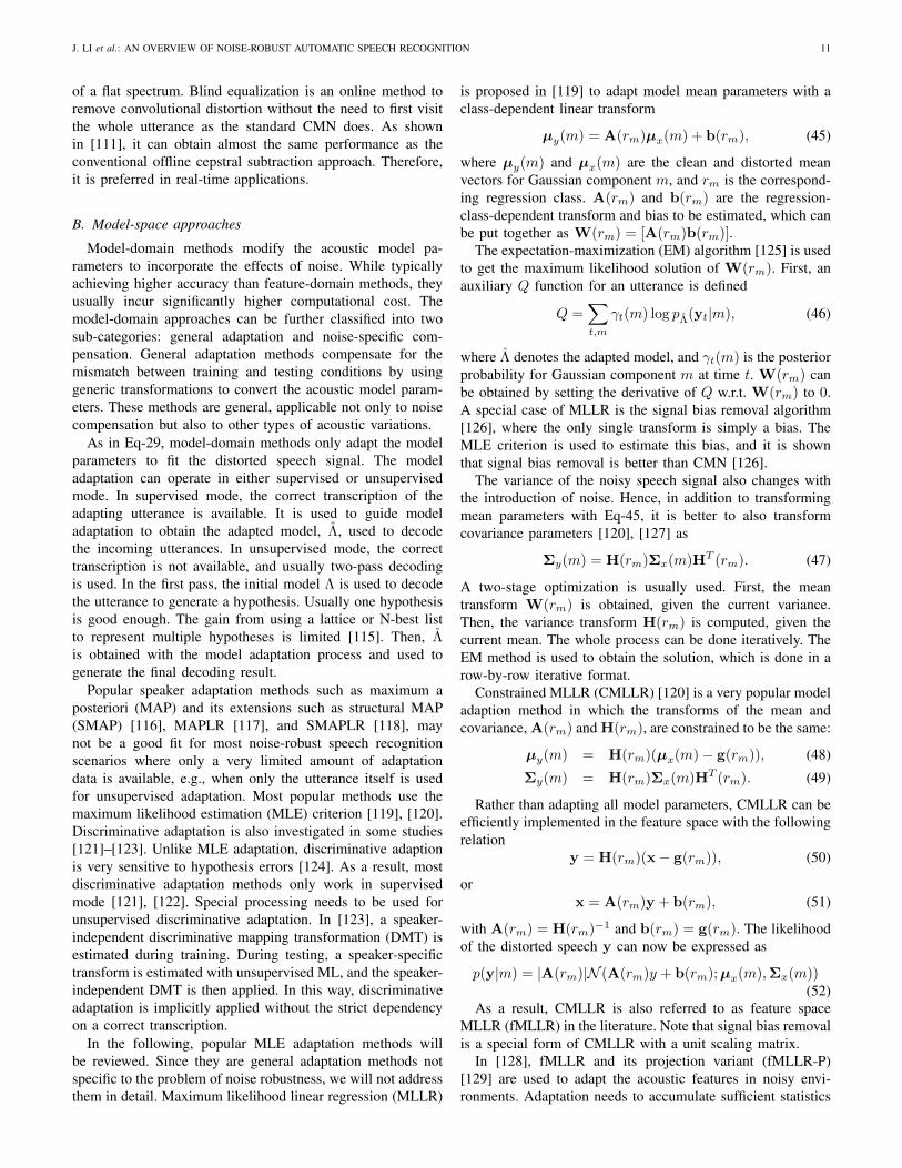
In the following, popular MLE adaptation methods willbe reviewed. Since they are general adaptation methods notspecific to the problem of noise robustness, we will not addressthem in detail. Maximum likelihood linear regression (MLLR)
is proposed in [119] to adapt model mean parameters with aclass-dependent linear transform
µy(m) = A(rm)µx(m) + b(rm), (45)
where µy(m) and µx(m) are the clean and distorted meanvectors for Gaussian component m, and rm is the correspond-ing regression class. A(rm) and b(rm) are the regression-class-dependent transform and bias to be estimated, which canbe put together as W(rm) = [A(rm)b(rm)].
The expectation-maximization (EM) algorithm [125] is usedto get the maximum likelihood solution of W(rm). First, anauxiliary Q function for an utterance is defined
Q =∑t,m
γt(m) log pΛ(yt|m), (46)
where Λ denotes the adapted model, and γt(m) is the posteriorprobability for Gaussian component m at time t. W(rm) canbe obtained by setting the derivative of Q w.r.t. W(rm) to 0.A special case of MLLR is the signal bias removal algorithm[126], where the only single transform is simply a bias. TheMLE criterion is used to estimate this bias, and it is shownthat signal bias removal is better than CMN [126].
The variance of the noisy speech signal also changes withthe introduction of noise. Hence, in addition to transformingmean parameters with Eq-45, it is better to also transformcovariance parameters [120], [127] as
Σy(m) = H(rm)Σx(m)HT (rm). (47)
A two-stage optimization is usually used. First, the meantransform W(rm) is obtained, given the current variance.Then, the variance transform H(rm) is computed, given thecurrent mean. The whole process can be done iteratively. TheEM method is used to obtain the solution, which is done in arow-by-row iterative format.
Constrained MLLR (CMLLR) [120] is a very popular modeladaption method in which the transforms of the mean andcovariance, A(rm) and H(rm), are constrained to be the same:
µy(m) = H(rm)(µx(m)− g(rm)), (48)
Σy(m) = H(rm)Σx(m)HT (rm). (49)
Rather than adapting all model parameters, CMLLR can beefficiently implemented in the feature space with the followingrelation
y = H(rm)(x− g(rm)), (50)
orx = A(rm)y + b(rm), (51)
with A(rm) = H(rm)−1 and b(rm) = g(rm). The likelihoodof the distorted speech y can now be expressed as
p(y|m) = |A(rm)|N (A(rm)y + b(rm);µx(m),Σx(m))(52)
As a result, CMLLR is also referred to as feature spaceMLLR (fMLLR) in the literature. Note that signal bias removalis a special form of CMLLR with a unit scaling matrix.
In [128], fMLLR and its projection variant (fMLLR-P)[129] are used to adapt the acoustic features in noisy envi-ronments. Adaptation needs to accumulate sufficient statistics
12 IEEE TRANS. AUDIO, SPEECH, AND LANGUAGE PROCESSING, VOL. X, NO. X, XXX 2013
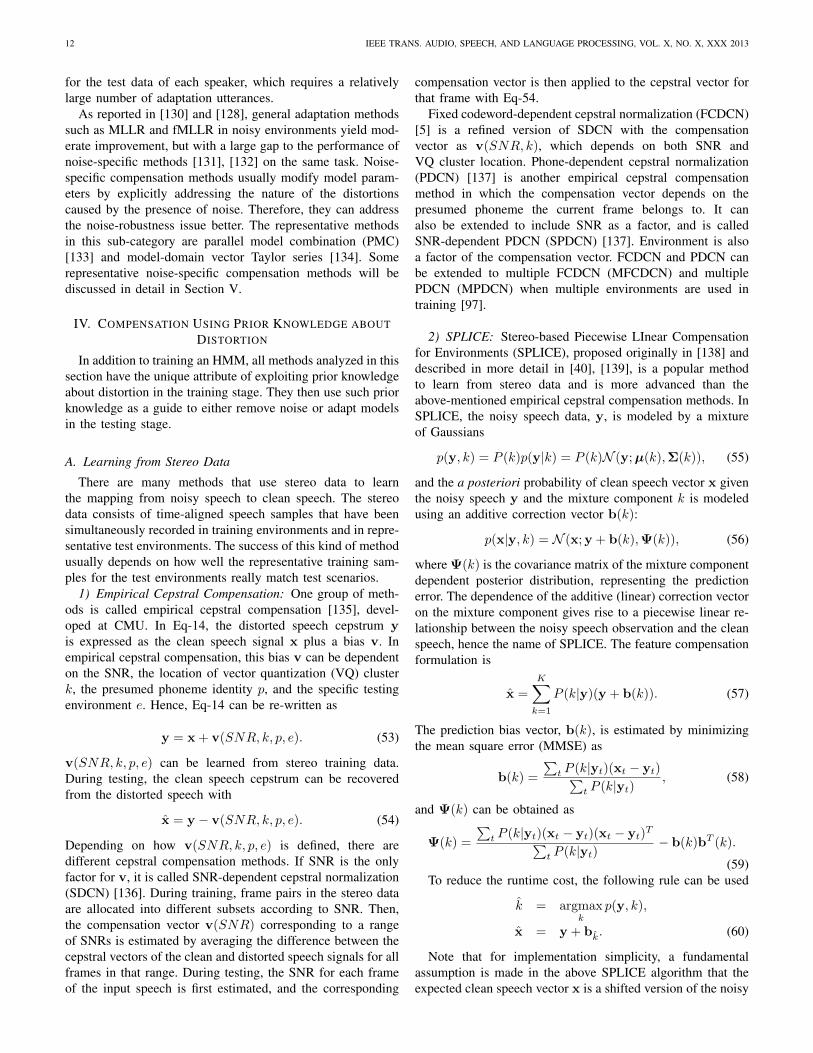
for the test data of each speaker, which requires a relativelylarge number of adaptation utterances.
As reported in [130] and [128], general adaptation methodssuch as MLLR and fMLLR in noisy environments yield mod-erate improvement, but with a large gap to the performance ofnoise-specific methods [131], [132] on the same task. Noise-specific compensation methods usually modify model param-eters by explicitly addressing the nature of the distortionscaused by the presence of noise. Therefore, they can addressthe noise-robustness issue better. The representative methodsin this sub-category are parallel model combination (PMC)[133] and model-domain vector Taylor series [134]. Somerepresentative noise-specific compensation methods will bediscussed in detail in Section V.
IV. COMPENSATION USING PRIOR KNOWLEDGE ABOUTDISTORTION
In addition to training an HMM, all methods analyzed in thissection have the unique attribute of exploiting prior knowledgeabout distortion in the training stage. They then use such priorknowledge as a guide to either remove noise or adapt modelsin the testing stage.
A. Learning from Stereo Data
There are many methods that use stereo data to learnthe mapping from noisy speech to clean speech. The stereodata consists of time-aligned speech samples that have beensimultaneously recorded in training environments and in repre-sentative test environments. The success of this kind of methodusually depends on how well the representative training sam-ples for the test environments really match test scenarios.
1) Empirical Cepstral Compensation: One group of meth-ods is called empirical cepstral compensation [135], devel-oped at CMU. In Eq-14, the distorted speech cepstrum yis expressed as the clean speech signal x plus a bias v. Inempirical cepstral compensation, this bias v can be dependenton the SNR, the location of vector quantization (VQ) clusterk, the presumed phoneme identity p, and the specific testingenvironment e. Hence, Eq-14 can be re-written as
y = x + v(SNR, k, p, e). (53)
v(SNR, k, p, e) can be learned from stereo training data.During testing, the clean speech cepstrum can be recoveredfrom the distorted speech with
x = y − v(SNR, k, p, e). (54)
Depending on how v(SNR, k, p, e) is defined, there aredifferent cepstral compensation methods. If SNR is the onlyfactor for v, it is called SNR-dependent cepstral normalization(SDCN) [136]. During training, frame pairs in the stereo dataare allocated into different subsets according to SNR. Then,the compensation vector v(SNR) corresponding to a rangeof SNRs is estimated by averaging the difference between thecepstral vectors of the clean and distorted speech signals for allframes in that range. During testing, the SNR for each frameof the input speech is first estimated, and the corresponding
compensation vector is then applied to the cepstral vector forthat frame with Eq-54.
Fixed codeword-dependent cepstral normalization (FCDCN)[5] is a refined version of SDCN with the compensationvector as v(SNR, k), which depends on both SNR andVQ cluster location. Phone-dependent cepstral normalization(PDCN) [137] is another empirical cepstral compensationmethod in which the compensation vector depends on thepresumed phoneme the current frame belongs to. It canalso be extended to include SNR as a factor, and is calledSNR-dependent PDCN (SPDCN) [137]. Environment is alsoa factor of the compensation vector. FCDCN and PDCN canbe extended to multiple FCDCN (MFCDCN) and multiplePDCN (MPDCN) when multiple environments are used intraining [97].
2) SPLICE: Stereo-based Piecewise LInear Compensationfor Environments (SPLICE), proposed originally in [138] anddescribed in more detail in [40], [139], is a popular methodto learn from stereo data and is more advanced than theabove-mentioned empirical cepstral compensation methods. InSPLICE, the noisy speech data, y, is modeled by a mixtureof Gaussians
p(y, k) = P (k)p(y|k) = P (k)N (y;µ(k),Σ(k)), (55)
and the a posteriori probability of clean speech vector x giventhe noisy speech y and the mixture component k is modeledusing an additive correction vector b(k):
p(x|y, k) = N (x; y + b(k),Ψ(k)), (56)
where Ψ(k) is the covariance matrix of the mixture componentdependent posterior distribution, representing the predictionerror. The dependence of the additive (linear) correction vectoron the mixture component gives rise to a piecewise linear re-lationship between the noisy speech observation and the cleanspeech, hence the name of SPLICE. The feature compensationformulation is
x =
K∑k=1
P (k|y)(y + b(k)). (57)
The prediction bias vector, b(k), is estimated by minimizingthe mean square error (MMSE) as
b(k) =
∑t P (k|yt)(xt − yt)∑
t P (k|yt), (58)
and Ψ(k) can be obtained as
Ψ(k) =
∑t P (k|yt)(xt − yt)(xt − yt)
T∑t P (k|yt)
− b(k)bT (k).
(59)To reduce the runtime cost, the following rule can be used
k = argmaxk
p(y, k),
x = y + bk. (60)
Note that for implementation simplicity, a fundamentalassumption is made in the above SPLICE algorithm that theexpected clean speech vector x is a shifted version of the noisy
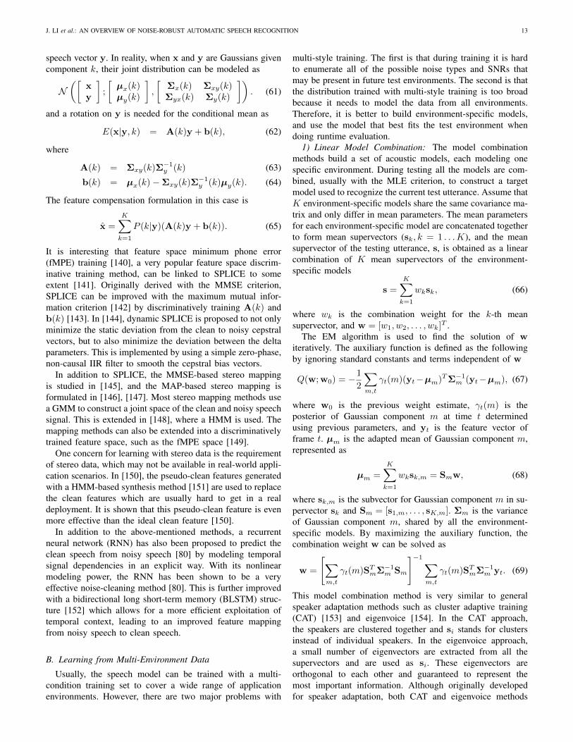
J. LI et al.: AN OVERVIEW OF NOISE-ROBUST AUTOMATIC SPEECH RECOGNITION 13
speech vector y. In reality, when x and y are Gaussians givencomponent k, their joint distribution can be modeled as
N([
xy
];
[µx(k)µy(k)
],
[Σx(k) Σxy(k)Σyx(k) Σy(k)
]). (61)
and a rotation on y is needed for the conditional mean as
E(x|y, k) = A(k)y + b(k), (62)
where
A(k) = Σxy(k)Σ−1y (k) (63)
b(k) = µx(k)−Σxy(k)Σ−1y (k)µy(k). (64)
The feature compensation formulation in this case is
x =
K∑k=1
P (k|y)(A(k)y + b(k)). (65)
It is interesting that feature space minimum phone error(fMPE) training [140], a very popular feature space discrim-inative training method, can be linked to SPLICE to someextent [141]. Originally derived with the MMSE criterion,SPLICE can be improved with the maximum mutual infor-mation criterion [142] by discriminatively training A(k) andb(k) [143]. In [144], dynamic SPLICE is proposed to not onlyminimize the static deviation from the clean to noisy cepstralvectors, but to also minimize the deviation between the deltaparameters. This is implemented by using a simple zero-phase,non-causal IIR filter to smooth the cepstral bias vectors.
In addition to SPLICE, the MMSE-based stereo mappingis studied in [145], and the MAP-based stereo mapping isformulated in [146], [147]. Most stereo mapping methods usea GMM to construct a joint space of the clean and noisy speechsignal. This is extended in [148], where a HMM is used. Themapping methods can also be extended into a discriminativelytrained feature space, such as the fMPE space [149].
One concern for learning with stereo data is the requirementof stereo data, which may not be available in real-world appli-cation scenarios. In [150], the pseudo-clean features generatedwith a HMM-based synthesis method [151] are used to replacethe clean features which are usually hard to get in a realdeployment. It is shown that this pseudo-clean feature is evenmore effective than the ideal clean feature [150].
In addition to the above-mentioned methods, a recurrentneural network (RNN) has also been proposed to predict theclean speech from noisy speech [80] by modeling temporalsignal dependencies in an explicit way. With its nonlinearmodeling power, the RNN has been shown to be a veryeffective noise-cleaning method [80]. This is further improvedwith a bidirectional long short-term memory (BLSTM) struc-ture [152] which allows for a more efficient exploitation oftemporal context, leading to an improved feature mappingfrom noisy speech to clean speech.
B. Learning from Multi-Environment Data
Usually, the speech model can be trained with a multi-condition training set to cover a wide range of applicationenvironments. However, there are two major problems with
multi-style training. The first is that during training it is hardto enumerate all of the possible noise types and SNRs thatmay be present in future test environments. The second is thatthe distribution trained with multi-style training is too broadbecause it needs to model the data from all environments.Therefore, it is better to build environment-specific models,and use the model that best fits the test environment whendoing runtime evaluation.
1) Linear Model Combination: The model combinationmethods build a set of acoustic models, each modeling onespecific environment. During testing all the models are com-bined, usually with the MLE criterion, to construct a targetmodel used to recognize the current test utterance. Assume thatK environment-specific models share the same covariance ma-trix and only differ in mean parameters. The mean parametersfor each environment-specific model are concatenated togetherto form mean supervectors (sk, k = 1 . . .K), and the meansupervector of the testing utterance, s, is obtained as a linearcombination of K mean supervectors of the environment-specific models
s =
K∑k=1
wksk, (66)
where wk is the combination weight for the k-th meansupervector, and w = [w1, w2, . . . , wk]T .
The EM algorithm is used to find the solution of witeratively. The auxiliary function is defined as the followingby ignoring standard constants and terms independent of w
Q(w; w0) = −1
2
∑m,t
γt(m)(yt−µm)TΣ−1m (yt−µm), (67)
where w0 is the previous weight estimate, γt(m) is theposterior of Gaussian component m at time t determinedusing previous parameters, and yt is the feature vector offrame t. µm is the adapted mean of Gaussian component m,represented as
µm =
K∑k=1
wksk,m = Smw, (68)
where sk,m is the subvector for Gaussian component m in su-pervector sk and Sm = [s1,m, . . . , sK,m]. Σm is the varianceof Gaussian component m, shared by all the environment-specific models. By maximizing the auxiliary function, thecombination weight w can be solved as
w =
[∑m,t
γt(m)STmΣ−1m Sm
]−1∑m,t
γt(m)STmΣ−1m yt. (69)
This model combination method is very similar to generalspeaker adaptation methods such as cluster adaptive training(CAT) [153] and eigenvoice [154]. In the CAT approach,the speakers are clustered together and si stands for clustersinstead of individual speakers. In the eigenvoice approach,a small number of eigenvectors are extracted from all thesupervectors and are used as si. These eigenvectors areorthogonal to each other and guaranteed to represent themost important information. Although originally developedfor speaker adaptation, both CAT and eigenvoice methods

14 IEEE TRANS. AUDIO, SPEECH, AND LANGUAGE PROCESSING, VOL. X, NO. X, XXX 2013
can be used for noise-robust speech recognition. Storing Ksupervectors in memory during online model combination maybe too demanding. One way to reduce the cost is to usemethods such as eigenMLLR [155], [156] and transform-basedCAT [153] by adapting a canonical mean with environmentdependent transforms. In this way, only K transforms arestored in memory. Moreover, adaptive training can be usedto find the canonical mean as in CAT [153].
One potential problem of ML model combination is thatusually all combination weights are not zero, i.e., everyenvironment-dependent model contributes to the final model.This is obviously not optimal if the test environment is exactlythe same as one of the training environments. There is also ascenario where the test environment can be approximated wellby interpolating only few training environments. Includingunrelated models into the construction brings unnecessarydistortion to the target model. This can be solved by ensemblespeaker and speaking environment modeling [157], in whichan online cluster selection is first used to locate the mostrelevant cluster and then only the supervectors in this selectedcluster contribute to the model combination. Another way isto use Lasso (least absolute shrinkage and selection operator)[158] to impose an L1 regularization term in the weightestimation problem. In [159], it is shown that Lasso usuallyshrinks the weights of the mean supervectors not relevant tothe test environment to zero. By removing some irrelevantsupervectors, the resulting mean supervectors are found to bemore robust to noise distortions.
Note that the noisy speech signal variance changes withthe introduction of noise, therefore simply adjusting the meanvector of the speech model cannot solve all of the problems.It is better to adjust the model variance as well. One wayis to combine the pre-trained CMLLR matrices as in [160].However, this is not trivial, requiring numerical optimizationmethods, such as the gradient descent method or a Newtonmethod as in [160].
2) Source Separation: In Section IV-B1, the acoustic modelfor the current test utterance is obtained by combining the pre-trained acoustic models. Recently, there is increasing interestto use exemplar-based methods for general ASR [161], [162]and noise-robust ASR [163]–[165]. Exemplar refers to an ex-ample speech segment from the training corpus. In exemplar-based noise-robust ASR [163]–[165], noisy speech is modeledby a linear combination of speech and noise [163], [165] (orother interfering factors, such as music [164]) exemplars. Ifthe reconstructed speech consists of only the exemplars ofclean speech, the impact of noise is removed. This is a sourceseparation approach, and non-negative matrix factorization(NMF) [166] has been shown to be a very successful method[167], [168], and can directly benefit noise-robust ASR [163]–[165], [169]. The source separation process with NMF isdescribed below.
First the training corpus is used to create a dictionaryxl(1 ≤ l ≤ L) of clean speech exemplars and a matrix Xis formed as X = [x1x2 . . .xL]. The exemplars are drawnrandomly from a collection of magnitude spectral vectors in atraining set. Similarly, the noise matrix N is formed with noise
exemplars. Then speech and noise exemplars are concatenatedtogether to form a single matrix A = [XN], with a total of Kexemplars. The exemplars of A are denoted Ak, 1 ≤ k ≤ K.The reconstruction signal is
y =
K∑k=1
wkAk = Aw, s.t. wk ≥ 0 (70)
with w as the K-dimension activation vector. All exemplarsand activation weights are non-negative. The objective is tominimize the reconstruction error d(y,Aw) between the ob-servation y and the reconstruction signal y while constrainingthe matrices to be element-wise non-negative. It is also goodto embed sparsity into the objective function so that the noisyspeech can be represented as a combination of a small set ofexemplars. This is done by penalizing the nonzero entries ofw with the L1 norm of the activation vector w, weighted byelement-wise multiplication (operation .*) of a non-negativevector λ. Therefore the objective function is
d(y,Aw) + ||λ. ∗w||1 s.t. wk ≥ 0 (71)
If all the elements of λ are zero, there is no enforced sparsity[164]. Otherwise, sparsity is enforced [163], [165]. In [166],two measures are used for the reconstruction error, namelyEuclidean distance and divergence. In most speech-relatedwork [163]–[165], Kullback-Leibler (KL) divergence is usedto measure the reconstruction error.
d(y, y) =
E∑e=1
ye log
(yeye
)− ye + ye, (72)
where E is the vector dimension.To solve Eq-71, the entries of the vector w are initialized
to unity. Then Eq-71 can be minimized by iteratively applyingthe update rule [165]
w← w. ∗ (A(y./(Aw)))./(A1 + λ) (73)
with .∗ and ./ denoting element-wise multiplication and divi-sion, respectively. 1 is a vector with all elements set to 1.
After getting w, the clean speech feature can be recon-structed by simply combining all the speech exemplars withnonzero weights [167]. Good recognition performance hasbeen observed particulary at very low SNR (below 0 dB).Better results are reported by using the following filtering[164], [165], [170] as
x = y. ∗Axwx./(Axwx + Anwn), (74)
where Ax and wx denote the exemplars and activation vectorfor clean speech, respectively, and An and wn denote theexemplars and activation vector for noise, respectively. This isreferred as feature enhancement (FE) in [165], [170].
Instead of cleaning the noisy speech magnitude spectrum,a sparse classification (SC) method is proposed in [163] todirectly use the activation weights to estimate the state orword likelihood. Since each frame of each speech exemplar inthe speech dictionary has state or word labels obtained fromthe alignment with conventional HMMs, the weights of theexemplars in the sparse representation wx can be used to

J. LI et al.: AN OVERVIEW OF NOISE-ROBUST AUTOMATIC SPEECH RECOGNITION 15
calculate the state or word likelihood. Then, these activation-based likelihoods are used in a Viterbi search to obtain thestate sequence with maximum likelihood.
Although the root methodology of FE and SC are thesame, i.e., NMF source separation, it is shown in [170],[171] that they are complementary. If combined together,more gain can be achieved. There are also variations ofstandard NMF source separation. For example, a sliding timewindow approach [172], that allows the exemplars to spanmultiple frames is used for decoding utterances of arbitrarylength. Convolutive extension of NMF is proposed to handlepotential dependencies across successive input columns [171],[173]. Prior knowledge of the co-occurrence statistics ofthe basis functions for each source can also be employedto improve the performance of NMF [174]. In [175],by minimizing cross-coherence between the dictionariesof all sources in the mixed signal, the bases set of onesource dictionary can be prevented from representing theother source signals. This clearly gives better separationresults than the traditional NMF. Superior digit recognitionaccuracy has been reported in [170] with the exemplar-basedmethod by increasing the number of update iterations andexemplars, designing artificial noise dictionary, doing noisesniffing, and combining SC with FE. An advantage of theexemplar-based approach is that it can deal with highlynon-stationary noise, such as speech recognition in thepresence of background music. However, there are still plentyof challenges. e.g., how to deal with convolutive channeldistortions, how to most effectively deal with noise types intesting that have not been previously seen in the developmentof the noise dictionary, and how to generalize to LVCSR tasks.
3) Variable-Parameter HMM: Variable-parameter HMM(VPHMM) [176] models the speech Gaussian mean andvariance parameters as a set of polynomial functions ofthe environment variable v, which is SNR in [176].Hence, the Gaussian component m is now modeled asN (y;µ(m, v),Σ(m, v)). µ(m, v) and Σ(m, v) are poly-nomial functions of environment variable v. For example,µ(m, v) can be denoted by
µ(m, v) =
P∑p=0
cp(m)vp, (75)
where cp(m) is a vector with the same dimension as theinput feature vectors. The choice of polynomial function isbased on its good approximation to continuous functions, itssimple derivation operations, and the fact that the change ofmeans and variances in terms of the environment is smoothand can be modeled by low order polynomials. Other functionscan also be used. For example, in [177], piecewise splineinterpolation is used to represent the dependency of the HMMparameters on the conditioning parameters. To reduce thetotal number of parameters for VPHMM, parameter clusteringcan be employed [178]. The VPHMM parameters can betrained either with the MLE criterion [176] or a discriminativecriterion [179]. In addition to Gaussian mean and varianceparameters, other model parameters can also be modeled.
In [180], [181], a more generalized form of VPHMM isinvestigated by modeling tied linear transforms as a functionof environment variables.
During testing, speech model parameters can be calculatedwith the estimated environment variable. Even if the estimatedenvironment is not seen during training, the curve fitting opti-mization naturally uses the information on articulation/contextfrom neighboring environments. Therefore, VPHMM canwork well in unseen environments.
V. EXPLICIT DISTORTION MODELING
An explicit distortion modeling method is a noise-robustnessmethod that employs a physical model of how distorted speechfeatures are generated. Because the physical constraints areexplicitly modeled, the explicit distortion modeling methodsrequire only a relatively small number of distortion parametersto be estimated. They also exhibit high noise-robustness per-formance due to the explicit modeling of the distorted speechgeneration process.
A. Parallel Model Combination
Parallel model combination (PMC) uses the explicit dis-tortion model to adapt the clean speech model. The modelparameters of clean speech and noise in the cepstral domainare first transformed to the log-Mel-filter-bank domain andfurther to the Mel-filter-bank domain. Then, the model pa-rameters of distorted speech in the Mel-filter-bank domaincan be calculated by using the explicit distortion model whichassumes that noise and clean speech are independent and addi-tive in the Mel-filter-bank domain. With either the log-normalapproximation [133] or the log-add approximation [133], themodel parameters of distorted speech in the log-Mel-filter-bank domain can be obtained and finally are transformed backto the cepstral domain with the DCT transform.
The basic PMC method can also be extended for situationswhere there is channel distortion as well as additive noise[133]. A simple technique presented in [133] uses a one statesingle Gaussian speech model to calculate the convolutivecomponent. An approximate solution of the convolutive com-ponent by steepest descent methods has also been reported[182], which relies on the Viterbi approximation and does nothandle mixture of Gaussian distributions. The method in [183]uses an additional universal speech Gaussian mixture modeland incorporates an existing bias estimation procedure [184]for channel estimation.
As shown in [185], the vector Taylor series (VTS) ap-proximation appears to be more accurate than the log-normalapproximation in PMC. Therefore, many studies of explicitdistortion modeling have switched to the VTS direction overthe last decade.
B. Vector Taylor Series
In recent years, a model-domain approach that jointlycompensates for additive and convolutive (JAC) distortions(e.g., [131], [132], [134], [185]–[189]) has yielded promisingresults. The various methods proposed so far use a parsimo-nious nonlinear physical model to describe the environmental

16 IEEE TRANS. AUDIO, SPEECH, AND LANGUAGE PROCESSING, VOL. X, NO. X, XXX 2013
distortion and use the VTS approximation technique to findclosed-form HMM adaptation and noise/channel parameterestimation formulas. Although some methods are referred towith different names, such as Jacobian adaptation [186] andJAC [131], [132], [188], they are in essence the VTS methodssince VTS is used to linearize the involved nonlinearity, fromwhich the solutions are derived.
Eq-14 is a popular nonlinear distortion model between cleanand distorted speech in the cepstral domain. It can be re-written as
y = x + h + g(x,h,n), (76)
where
g(x,h,n) = C log(1 + exp(C−1(n− x− h)))). (77)
In standard VTS adaptation [134], the nonlinear functionin Eq-77 is approximated using a first order VTS expansionat point (µx(m),µh,µn). µx(m), µn, and µh are the staticcepstral means of the clean speech Gaussian component m,noise, and channel, respectively.
Denoting
∂y
∂x|µx(m),µn,µh
=∂y
∂h|µx(m),µn,µh
= G(m), (78)
∂y
∂n|µx(m),µn,µh
= I−G(m) = F(m), (79)
where G(m) is the Jacobian matrix for Gaussian componentm, defined as
G(m)=Cdiag
(1
1 + exp(C−1(µn − µx(m)− µh))
)C−1,
(80)Eq-76 can then be approximated by a vector Taylor seriesexpansion, truncated after the linear term:
y|µx(m),µh,µn≈ µx(m) + µh + g(µx(m),µh,µn)
+G(m)(x− µx(m))+G(m)(h− µh)+F(m)(n− µn), (81)
With Eq-81, the distorted speech y is now a linear functionof the clean speech x, the noise n, and the channel h,in the cepstral domain. This linearity facilitates the HMMmodel adaptation and distortion parameter estimation byproviding possible closed-form solutions because a Gaussiandistribution, dominantly used in ASR, with linear operationis still a Gaussian distribution.
1) Vector Taylor Series Model Adaptation: By taking theexpectation on both sides of Eq-81, the static mean of thedistorted speech signal µy for Gaussian component m can bewritten as
µy(m) ≈ µx(m) + µh + g(µx(m),µh,µn), (82)
and the static variance of the distorted speech signal µy forGaussian component m can be obtained by taking the varianceoperation on both sides of Eq-81:
Σy(m) ≈ diag(G(m)Σx(m)G(m)T + F(m)ΣnF(m)T ),(83)
The delta parameters can be updated [185] with the contin-uous time approximation [190]:
µ∆y(m) ≈ G(m)µ∆x(m), (84)
Σ∆y(m) ≈ diag(G(m)Σ∆x(m)G(m)T
+F(m)Σ∆nF(m)T), (85)
The delta-delta model parameters are updated similarly.Note that although the cepstral distortion formulation,
i.e., Eq-14, is widely used in VTS studies, the log spectraldistortion formulation, i.e., Eq-13, can also be used [188].Some studies [191] even work in the linear frequencydomain. However, this brings a large computational cost andthe diagonal covariance assumption used in [191] may not bevalid for linear frequency. Therefore, there are only a smallnumber of VTS methods working in the linear frequencydomain.
2) Distortion Estimation in VTS: Although proposed in1996 [134], VTS model adaptation has shown great accuracyadvantages over other noise-robustness methods only recently[131], [132] when the distortion model parameters are re-estimated based on the first-pass decoding result with theexpectation-maximization (EM) algorithm [131], [132]. First,an auxiliary Q function for an utterance is
Q =∑t,m
γt(m) log pΛ(yt|m), (86)
where Λ denotes the adapted model, and γt(m) is the posteriorprobability for the Gaussian component m of the HMM, i.e.,
γt(m) = pΛ0(m|Y), (87)
where Λ0 denotes the previous model.To maximize the auxiliary function in the M-step of the EM
algorithm, the derivatives of Q are taken with respect to µnand µh, and are set to 0. Then, the mean of the noise µn canbe updated according to [132]:
µn = µn,0 + A−1n bn, (88)
with
An =∑t,m
γt(m)F(m)TΣ−1y (m)F(m), (89)
bn =∑t,m
γt(m)F(m)TΣ−1y (m)(yt − µy,0(m)), (90)
µy,0(m) = µx(m)− µh,0 − g(µx(m),µh,0,µn,0). (91)
where µn,0 and µh,0 are the VTS expansion points for µnand µh, respectively. The channel mean µh can be updatedsimilarly as in [132]. Newton’s method, an iterative secondorder approach, is used to estimate the noise variance [132].
Distortion parameter estimation can also be done in otherways. In [192], a gradient-descent method is used to obtainthe noise variance estimate. Since there is no guarantee thatthe auxiliary function will increase, a back-off step is needed.In [193], a Gauss-Newton method is used by discarding thesecond derivative of the residual with respect to the distortionparameters when calculating the Hessian. In [187], both the

J. LI et al.: AN OVERVIEW OF NOISE-ROBUST AUTOMATIC SPEECH RECOGNITION 17
static mean and variance parameters in the cepstral domain areadjusted using the VTS approximation technique. In that work,however, noise was estimated on a frame-by-frame basis,which is complex and computationally costly. It is shown in[194] that the estimation method used in this section [131],[132] is clearly better than the estimation method in [187].
3) VTS Feature Enhancement: As shown in [132], VTSmodel adaptation achieves much better accuracy than severalpopular model adaptation technologies. Although VTS modeladaptation can achieve high accuracy, the computational costis very high as all the Gaussian parameters in the recognizerneed to be updated every time the environmental parameterschange. This time-consuming requirement hinders VTS modeladaptation from being widely used, especially in LVCSR taskswhere the number of model parameters is large.
On the other hand, VTS feature enhancement has beenproposed as a lower-cost alternative to VTS model adaptation.For example, a number of techniques have been proposedthat can be categorized as model-based feature enhancementschemes [134], [195]–[197]. These methods use a small GMMin the front-end and the same methodology used in VTS modeladaptation to derive a minimum-mean-square-error (MMSE)estimate of the clean speech features given the noisy obser-vations. In addition to the advantage of a low runtime cost,VTS feature enhancement can be easily combined with otherpopular feature-based technologies, such as CMN, HLDA,fMPE, etc., which are challenging to VTS model adaptation.
In general, the MMSE method can be used to get theestimate of clean speech
x = E(x|y) =
∫xp(x|y)dx. (92)
Denote the clean-trained GMM as
pΛ(x) =
K∑k=1
c(k)N (x;µx(k),Σx(k)), (93)
along with Eq-14, the MMSE estimate of clean speech be-comes
x = y − h−K∑k=1
P (k|y)∫C log(1 + exp(C−1(n− x− h)))p(x|y, k)dx,(94)
where P (k|y) is the Gaussian posterior probability, calculatedas
P (k|y) =c(k)N (y;µy(k),Σy(k))∑Kk=1 c(k)N (y;µy(k),Σy(k))
. (95)
If the 0th-order VTS approximation is used for the nonlinearterm in Eq-94, the MMSE estimate of cleaned speech x isobtained as
x = y−h−K∑k=1
P (k|y)C log(1+exp(C−1(µn−µx(k)−µh))).
(96)
This formulation was first proposed in [134]. In [195], anothersolution was proposed when expanding Eq-14 with the 1st-order VTS. For the kth GMM component, the joint distributionof x and y is modeled as Eq-61.
The following can be derived [195]
E(x|y, k) = µx|y(k) = µx(k)+Σxy(k)Σ−1y (k)(y−µy(k)).
(97)Then the MMSE estimate of clean speech is [195]
x =
K∑k=1
P (k|y)(µx(k) + Σx(k)G(k)
TΣ−1y (k)(y − µy(k))
).
(98)Two key aspects of VTS feature enhancement are how to
obtain reliable estimates of the noise and channel distortionparameters and how to accurately calculate the Gaussian oc-cupancy probability. In contrast to using static features alone tocalculate the Gaussian occupancy probability [189], both staticand dynamic features are used to obtain more reliable Gaussianoccupancy probabilities. Then, these probabilities are pluggedinto Eq-96 or Eq-98. In [198], it is shown that recent improve-ments in VTS model adaptation can be incorporated into VTSfeature enhancement to improve the algorithm performance:Updating all of the environment distortion parameters [131]and subsequently carrying out noise adaptive training [199].
A common concern of feature enhancement is that afterthe enhancement, the clean speech signal is distorted and theaccuracy on clean testing will drop. As shown in [200], VTSfeature enhancement enjoys the nice property that it signif-icantly improves accuracy in noisy test conditions withoutdegrading accuracy in clean test conditions.
By incorporating the recent advances in VTS modeladaptation, VTS feature enhancement can obtain very highaccuracy on some noisy tasks [198]. However, it is shownthat there is still a small accuracy gap between VTS featureenhancement and VTS model adaptation [198]. Regarding theruntime cost, VTS model adaptation needs to adapt HMMparameters twice, while VTS feature enhancement needsto adapt GMM parameters twice. Usually, the number ofparameters in a front-end GMM is much smaller than that inthe back-end HMM. Furthermore, two rounds of decodingare needed in VTS model adaptation while only one roundof decoding is performed in VTS feature enhancement. Asa consequence, VTS feature enhancement has a much lowercomputational cost than VTS model adaptation. Therefore,the tradeoff between accuracy and computational cost willdetermine which technology is more suitable in a real worlddeployment scenario.
4) Improvements over VTS: Recently, there has been a se-ries of studies focusing on how to improve the performance ofVTS. A natural extension to the VTS methods described in theprevious section is to use high-order VTS expansion insteadof first-order VTS expansion. That way, the nonlinear relationfound in Eq-14 can be well modeled. There are several studies[201]–[203] along this line. As shown in [203], the 2nd-orderVTS is shown to achieve a noticeable performance gain overthe 1st-order VTS, although the accuracy gap between the

18 IEEE TRANS. AUDIO, SPEECH, AND LANGUAGE PROCESSING, VOL. X, NO. X, XXX 2013
3rd-order VTS and 2nd-order VTS is small. Another way toaddress the inaccuracy problem of the first-order Taylor seriesexpansion in the VTS is to use piecewise functions to modelthe nonlinearity, such as a piecewise linear approximation[204] or linear spline interpolation [205].
Eq-14 is simplified from Eq-12 of the phase-sensitivemodel, by approximating α[l] as 0 [19]. There is some work[202] that uses the phase-sensitive model for better modelingof the distortion. α can be estimated from the training set[202]. Due to its physical interpretation, the value of elementsin α ranges from -1 to 1. In [206], this value constraint isbroken by assigning a constant value α to the elements of α.If α is set to 0 and 1, VTS can be considered to work withMFCCs extracted from the power spectrum and magnitudespectrum, respectively [132]. It is shown in [206] that the bestaccuracy is obtained on the Aurora 2 task when the valueis set to around 2.5, which is larger than 1, the theoreticalmaximum value. Similar observations are also reported inlater work [207], [208]. Therefore, the phase-sensitive modelwith a constant α value can also be considered to be ageneralization function of the distortion model. The phase-sensitive model with a large α value may be consideredas a way to compensate the loss brought by the inaccurateapproximation in VTS. Another way to handle the phase termis to use the ALGONQUIN algorithm [209], which modelsthe phase term as the modeling error with Eq-76.
In standard VTS, the delta and delta-delta model parametersare updated [185] with the continuous time approximation[190], which makes the assumption that the dynamic cepstralcoefficients are the time derivatives of the static cepstralcoefficients. In [210], extended VTS is proposed to providea more accurate form to adapt dynamic model parameters.Extended VTS has been shown to outperform standard VTSwith the cost of more expensive computation [210].
As mentioned before, high computational cost is a concernfor VTS model adaptation. Feature VTS enhancement usesa small GMM on the front-end and the same methodologyused in VTS model adaptation to derive a MMSE estimateof the clean speech features given the noisy observations.However, even after employing the recent advanced methodsin VTS model adaptation, feature VTS enhancement stillhas an obvious accuracy gap between it and VTS modeladaptation [198]. In [200], VTS model adaptation with adiagonal Jacobian approximation method is proposed to havea relatively small accuracy loss and to offer a drastic savingsin computational cost over all three major components in stan-dard VTS model adaptation. The computational cost reductionis on a scale of O(D) for the Jacobian calculation and mostparts of parameter adaptation, and O(D2) for online distortionestimation, where D is the dimension of static cepstral feature.There is also a family of joint uncertainty decoding (JUD)methods [211]–[213] that can reduce the computational cost ofVTS by changing the Jacobian in Eq-80 from being Gaussian-dependent to regression-class-dependent. We will discuss thesemethods in Section VI-C2.
C. Sampling-Based Methods
The PMC methods in Section V-A rely on either the log-normal or the log-add approximation while the VTS methodsin Section V-B rely on the first-order or higher-order VTSapproximation. These approximations inevitably cause lossin model adaptation or feature enhancement. To improvethe implementation accuracy of explicit distortion modeling,sampling-based methods can be used.
1) Data-Driven PMC: Data-driven parallel model combi-nation (DPMC) [133] can be used to improve the modelingaccuracy of PMC. This method is based on Monte-Carlo(MC) sampling by drawing random samples from the cleanspeech and noise distributions. In a non-iterative DPMC,the frame/state component alignment within a state does notchange, and the clean speech samples are drawn from eachGaussian of the clean speech distributions.
x(m) ∼ N (µx(m),Σx(m))
n ∼ N (µn,Σn) (99)
Then, the distorted speech samples can be obtained with Eq-14, and the static mean and variance of the distorted speechfor Gaussian component m are estimated as the sample meanand variance of N distorted speech samples.
As N → ∞, the sample mean and covariance areapproaching the true values. However, due to the nature ofrandom sampling, N needs to be very large to guarantee theapproximation accuracy. Hence, the biggest disadvantage ofDPMC is the computational cost. As a solution, a modeladaptation method based on the unscented transform [214] isproposed in [215], [216].
2) Unscented Transform: Originally developed to improvethe extended Kalman filter and introduced to the field of robustASR in [215], [216], the unscented transform (UT) [214] givesan accurate estimate of the mean and variance parameters ofa Gaussian distribution under a nonlinear transformation bydrawing only a limited number of samples. This is achieved bysystematically drawing samples jointly from the clean speechand noise distributions, described in the following.
An augmented signal s = [xT ,nT ]T is formed with a D-dimensional clean speech cepstral vector x and a noise cepstralvector n, with dimensionality Ds = Dx +Dn = 2D. The UTalgorithm samples the Gaussian-dependent augmented signalwith 4D + 1 sigma points si(m).
In the feature space, the transformed sample yi(m) fromthe sigma point si(m) = [xi(m)T ,nT ]T is obtained with themapping function of Eq-14. Then, the static mean and varianceof the distorted speech are estimated as the sample mean andvariance of these 4D + 1 transformed samples.
It is shown in [214] that the UT accurately matches themean and covariance of the true distribution. Due to thespecial sampling strategy of the UT, the number of samplesto be computed, 4D + 1, is much smaller than N . Thereforemodel adaptation with the UT is more affordable than the MCmethod.
In [216], the static mean and variance of nonlinearlydistorted speech signals are estimated using the UT, but the

J. LI et al.: AN OVERVIEW OF NOISE-ROBUST AUTOMATIC SPEECH RECOGNITION 19
static noise mean and variance are estimated from a simpleaverage of the beginning and ending frames of the currentutterance. This technique was improved in [217], where thestatic noise parameters were estimated online with MLE usingthe VTS approximation and the estimates were subsequentlyplugged into the UT formulation to obtain the estimate ofthe mean and variance of the static distorted speech features.In [218], a robust feature extraction technique is proposedto estimate the parameters of the conditional noise andchannel distribution using the UT and embed the estimatedparameters into the EM framework. In all of these approaches[216]–[218], sufficient statistics of only the static featuresor model parameters are estimated using the UT althoughadaptation of the dynamic model parameters with reliablenoise and channel estimations has shown to be important[131], [132]. As a solution, an approach is proposed in [219]to unify static and dynamic model parameter adaptation withonline estimation of noise and channel parameters in the UTframework.
3) Methods Beyond the Gaussian Assumption: As shown inFigure 2, with the introduction of noise, the distorted speechis no longer Gaussian distributed. Therefore, the popularone-to-one Gaussian mapping used in the above-mentionedmethods has a theoretic flaw. The iterative DPMC method[133] solves this problem by sampling from GMMs insteadof Gaussians and then uses the Baum-Welch algorithm tore-estimate the distorted speech parameters. This is extendedin [220], where a variational method is used to removethe constraint that the samples must be used to model theGaussians they are originally drawn from. This is alsoextended to variational PCMLLR [220], which is shownto be better than PCMLLR [211] and has a much lowercomputational cost than variational DPMC. In [221] theGaussian at the input of the nonlinearity is approximatedby a GMM whose individual components have a smallervariance than the original Gaussian. A VTS linearization ofthe individual GMM components then incurs fewer errorsthan the linearization of the original Gaussian. Thus theoverall modeling accuracy could be improved.
The explicit distortion modeling methods discussed in thissection separate the clean speech feature from the environment(noise and channel) factors. This can be further extended toan acoustic factorization [222] problem: separate the cleanspeech feature/model from the multiple speaker and environ-mental factors irrelevant to the phonetic classification. Thereare plenty of recent studies addressing acoustic factorization[223]–[228].
From the work on explicit distortion modeling and acousticfactorization, we can see the trend of building increasinglysophisticated models to characterize the impact of differentdistortion sources, such as noise, channel, and speaker, onclean speech. Importantly, these better and better explicit dis-tortion models and the related techniques are already providingoutstanding performance which is superior to other methodsexploiting less powerful distortion models. A greater perfor-mance gap is expected in the future as more advanced explicit
distortion models are being developed and incorporated intonoise-robust ASR methods.
VI. COMPENSATION WITH UNCERTAINTY PROCESSING
The effects of strong noise necessarily create inherentuncertainty, either in the feature or model space, which can bebeneficially integrated into the popular plug-in MAP decod-ing in the ASR process. When a noise-robust method takesinto consideration that uncertainty, we call it an uncertaintyprocessing method.
A. Model-Domain Uncertainty
Uncertainty in the HMM parameters has been representedby their statistical distribution [229]. In order to take advantageof the model parameter uncertainty, the decision rule forrecognition can be improved from the conventional MAPdecision rule in Eq-100
W = argmaxW
pΛ(Y|W)PΓ(W). (100)
to the minimax decision rule [230]1
W = argmaxW
(PΓ(W) max
Λ∈ΩpΛ(Y|W)
), (101)
or to the Bayesian prediction classification (BPC) rule [231],[232]
W = argmaxW
(∫Λ∈Ω
pΛ(Y|W)p(Λ|φ,W)dΛ
)PΓ(W),
(102)where φ is the hyper-parameter characterizing the distributionof acoustic model parameter Λ, and Ω denotes the spacethat Λ lies in. Both minimax classification and BPC considerthe uncertainty of the estimated model, reflected by Ω. Theychange the decision rule to address this uncertainty usingtwo steps. In the first step, either the maximum value ofpΛ(Y|W) within the parameter neighborhood (as in minimaxclassification) or the integration of pΛ(Y|W) in this parameterneighborhood (as in BPC) for word W is obtained. In thesecond step, the value obtained in the first step is pluggedinto the MAP decision rule.
It is usually difficult to define the parameter neighborhoodΩ. Moreover, with two-stage processing the computationalcost of model space uncertainty using the modified decisionrule is very large. It usually involves a very complicatedimplementation, which prevents this type of method frombeing widely used although there was some research intominimax classification [230], [233] and BPC [231], [232] untilaround 10 years ago. An alternative treatment of uncertaintyis by integrating over the feature space instead of over themodel space. This will offer a much simpler system imple-mentation and lower computational cost. Therefore, researchhas switched to feature space uncertainty or joint uncertaintydecoding as described in the following sections.
1This is derived from minimizing the upper bound of the worse-caseprobability of classification error.
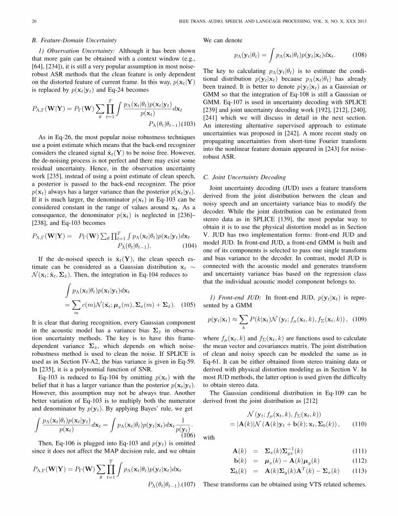
20 IEEE TRANS. AUDIO, SPEECH, AND LANGUAGE PROCESSING, VOL. X, NO. X, XXX 2013
B. Feature-Domain Uncertainty
1) Observation Uncertainty: Although it has been shownthat more gain can be obtained with a context window (e.g.,[64], [234]), it is still a very popular assumption in most noise-robust ASR methods that the clean feature is only dependenton the distorted feature of current frame. In this way, p(xt|Y)is replaced by p(xt|yt) and Eq-24 becomes
PΛ,Γ(W|Y) = PΓ(W)∑θ
T∏t=1
∫pΛ(xt|θt)p(xt|yt)
p(xt)dxt
PΛ(θt|θt−1).(103)
As in Eq-26, the most popular noise robustness techniquesuse a point estimate which means that the back-end recognizerconsiders the cleaned signal xt(Y) to be noise free. However,the de-noising process is not perfect and there may exist someresidual uncertainty. Hence, in the observation uncertaintywork [235], instead of using a point estimate of clean speech,a posterior is passed to the back-end recognizer. The priorp(xt) always has a larger variance than the posterior p(xt|yt).If it is much larger, the denominator p(xt) in Eq-103 can beconsidered constant in the range of values around xt. As aconsequence, the denominator p(xt) is neglected in [236]–[238], and Eq-103 becomes
PΛ,Γ(W|Y) = PΓ(W)∑θ
∏Tt=1
∫pΛ(xt|θt)p(xt|yt)dxt
PΛ(θt|θt−1). (104)
If the de-noised speech is xt(Y), the clean speech es-timate can be considered as a Gaussian distribution xt ∼N (xt; xt,Σx). Then, the integration in Eq-104 reduces to∫
pΛ(xt|θt)p(xt|yt)dxt
=∑m
c(m)N (xt;µx(m),Σx(m) + Σx). (105)
It is clear that during recognition, every Gaussian componentin the acoustic model has a variance bias Σx in observa-tion uncertainty methods. The key is to have this frame-dependent variance Σx, which depends on which noise-robustness method is used to clean the noise. If SPLICE isused as in Section IV-A2, the bias variance is given in Eq-59.In [235], it is a polynomial function of SNR.
Eq-103 is reduced to Eq-104 by omitting p(xt) with thebelief that it has a larger variance than the posterior p(xt|yt).However, this assumption may not be always true. Anotherbetter variation of Eq-103 is to multiply both the numeratorand denominator by p(yt). By applying Bayes’ rule, we get∫
pΛ(xt|θt)p(xt|yt)p(xt)
dxt =
∫pΛ(xt|θt)p(yt|xt)dxt
1
p(yt).
(106)Then, Eq-106 is plugged into Eq-103 and p(yt) is omitted
since it does not affect the MAP decision rule, and we obtain
PΛ,Γ(W|Y) = PΓ(W)∑θ
T∏t=1
∫pΛ(xt|θt)p(yt|xt)dxt
PΛ(θt|θt−1).(107)
We can denote
pΛ(yt|θt) =
∫pΛ(xt|θt)p(yt|xt)dxt. (108)
The key to calculating pΛ(yt|θt) is to estimate the condi-tional distribution p(yt|xt) because pΛ(xt|θt) has alreadybeen trained. It is better to denote p(yt|xt) as a Gaussian orGMM so that the integration of Eq-108 is still a Gaussian orGMM. Eq-107 is used in uncertainty decoding with SPLICE[239] and joint uncertainty decoding work [192], [212], [240],[241] which we will discuss in detail in the next section.An interesting alternative supervised approach to estimateuncertainties was proposed in [242]. A more recent study onpropagating uncertainties from short-time Fourier transforminto the nonlinear feature domain appeared in [243] for noise-robust ASR.
C. Joint Uncertainty Decoding
Joint uncertainty decoding (JUD) uses a feature transformderived from the joint distribution between the clean andnoisy speech and an uncertainty variance bias to modify thedecoder. While the joint distribution can be estimated fromstereo data as in SPLICE [139], the most popular way toobtain it is to use the physical distortion model as in SectionV. JUD has two implementation forms: front-end JUD andmodel JUD. In front-end JUD, a front-end GMM is built andone of its components is selected to pass one single transformand bias variance to the decoder. In contrast, model JUD isconnected with the acoustic model and generates transformand uncertainty variance bias based on the regression classthat the individual acoustic model component belongs to.
1) Front-end JUD: In front-end JUD, p(yt|xt) is repre-sented by a GMM
p(yt|xt) ≈∑k
P (k|xt)N (yt; fµ(xt, k), fΣ(xt, k)) , (109)
where fµ(xt, k) and fΣ(xt, k) are functions used to calculatethe mean vector and covariances matrix. The joint distributionof clean and noisy speech can be modeled the same as inEq-61. It can be either obtained from stereo training data orderived with physical distortion modeling as in Section V. Inmost JUD methods, the latter option is used given the difficultyto obtain stereo data.
The Gaussian conditional distribution in Eq-109 can bederived front the joint distribution as [212]
N (yt; fµ(xt, k), fΣ(xt, k))
= |A(k)|N (A(k)yt + b(k); xt,Σb(k)) , (110)
with
A(k) = Σx(k)Σ−1yx (k) (111)
b(k) = µx(k)−A(k)µy(k) (112)
Σb(k) = A(k)Σy(k)AT (k)−Σx(k) (113)
These transforms can be obtained using VTS related schemes.

J. LI et al.: AN OVERVIEW OF NOISE-ROBUST AUTOMATIC SPEECH RECOGNITION 21
Using Eq-110 and a rough assumption that P (k|xt) ≈P (k|yt), Eq-108 can be re-written as [212]
pΛ(yt|θt) =∑k
∑m
c(m)P (k|yt)|A(k)|
N (A(k)yt + b(k);µx(m),Σx(m) + Σb(k)) (114)
The summation in Eq-114 is time consuming, involving theclean speech GMM component m and the front-end GMMcomponent k. One popular approach is to select the mostdominating front-end component k∗
k∗ = argmaxk
P (k|yt) (115)
and Eq-114 can be simplified as
pΛ(yt|θt) ≈∑m
c(m)|A(k∗)|
N (A(k∗)yt + b(k∗);µx(m),Σx(m) + Σb(k∗)) (116)
Comparing Eq-116 with Eq-105, we can see that front-enduncertainty decoding transfers the distorted feature yt inaddition to adding a variance bias. SPLICE with uncertaintydecoding [239] is similar to front-end JUD, but with a differentformat of A(k), b(k), and Σb(k).
As discussed in [212], [244], in low SNR conditions wherenoise dominates the speech signal, the conditional distributionp(yt|xt) degenerates to the distribution of additive noise ntas
p(yt|xt) ≈ N (nt;µn,Σn). (117)
Then the distribution of distorted speech in Eq-108 alsobecomes the distribution of additive noise
pΛ(yt|θt) = N (nt;µn,Σn). (118)
With Eq-118, the distribution of every state is thesame. Therefore, the current frame cannot contribute todifferentiating states using acoustic model scores. This is thebiggest theoretical issue with front-end uncertainty decoding,although SPLICE with uncertainty decoding can circumventthis issue with additional processing [239].
2) Model JUD: In front-end JUD, its conditional distribu-tion is completely decoupled from the acoustic model used forrecognition. In contrast, model JUD [192] links them togetherwith
p(yt|xt) ≈ N (yt; fµ(xt, rm), fΣ(xt, rm)) , (119)
where rm is the regression class index of acoustic modelGaussian component m, generated with the method in [245].The joint distribution of clean and noisy speech can bemodeled similarly as in Eq-61 by replacing the front-endcomponent index k with the regression class index rm. Witha similar derivation as in front-end JUD, the likelihood ofdistorted speech can be denoted by
pΛ(yt|θt) ≈∑m
c(m)|A(rm)|N (A(rm)yt + b(rm);
µx(m),Σx(m) + Σb(rm)) (120)
Comparing Eq-120 with Eq-116, we can tell that the differencebetween model JUD and front-end JUD is that in front-end JUD only the best component k∗ selected in front-endprocessing is passed to modify the likelihood evaluation duringdecoding while in model JUD every Gaussian component isassociated with a regression-class-dependent transform. There-fore, in model JUD, the distorted feature yt is transformedby multiple transforms, similar to CMLLR [120]. However,it differs from CMLLR due to the regression-class-dependentvariance term Σb(rm).
There are several extensions of model JUD. Σb(rm) in Eq-120 is a full covariance matrix. This brings a large computa-tional cost when evaluating the likelihood. One direct solutionis to diagonalize it, however, this solution turns out to havepoor performance [244]. Predictive CMLLR (PCMLLR) [211]can be used to avoid the full covariance matrix by applyinga CMLLR-like transform in the feature space transformed bymodel JUD
yt = A(rm)yt + b(rm). (121)
The likelihood for PCMLLR decoding is given by
pΛ(yt|θt) ≈∑m
c(m)|Ap(rm)||A(rm)|N (Ap(rm)yt
+ bp(rm);µx(m),Σx(m)) (122)
Ap(rm) and bp(rm) are obtained by using CMLLR, with thestatistics obtained from the model JUD transformed featureyt. With Eq-122, the clean acoustic model is unchanged.
Another alternative is with VTS-JUD [213], [246] in whichthe likelihood is computed as
pΛ(yt|θt) ≈∑m
c(m)N (yt; H(rm)(µx(m)− b(rm)),
diag(H(rm)(Σx(m) + Σb(rm))HT (rm))) (123)
where H(rm) = A−1(rm). VTS-JUD can be considered asthe model space implementation of model JUD, very similarto VTS but with less computational cost. In [247], noiseCMLLR is also proposed to extend the conventional CMLLRin Section III-B to reflect additional uncertainty from noisyfeatures by introducing a covariance bias with the same formas Eq-119. All of model JUD, VTS-JUD, and PCMLLR useVTS in Section V to calculate the regression-class-dependenttransforms. If the number of regression classes is identical tothe number of Gaussians, it can be proven that all of thesemethods are the same as VTS. By using regression classes,some computational cost can be saved. For example, in Eq-123 of VTS-JUD, although it still needs to apply transformsto every Gaussian mean and variance of the clean acousticmodel, the cost of calculating transforms is reduced becausethey are now regression-class-dependent instead of Gaussian-dependent.
Recently, subspace Gaussian mixture models (SGMM) areproposed in [248] with better performance than GMMs. In[249], an extension of JUD when using SGMMs is presentedwith good improvements in noisy conditions.

22 IEEE TRANS. AUDIO, SPEECH, AND LANGUAGE PROCESSING, VOL. X, NO. X, XXX 2013
D. Missing-Feature Approaches
Missing-feature approaches [250], [251], also known asmissing-data approaches, introduce the concept of uncertaintyinto feature processing. The methods are based on the inherentredundancy in the speech signal: one may still be able to recog-nize speech effectively even with only a fraction of the spectro-temporal information in the speech signal. They attempt todetermine which time-frequency cells are unreliable due tothe introduction of noise or other types of interference. Theseunreliable cells are either ignored or filled in by estimates oftheir putative values in subsequent processing [252], [253].
There are two major types of missing-feature approaches,namely, feature vector imputation and classifier modification[254]. Feature imputation methods treat unreliable spectralcomponents as missing components and attempt to reconstructthem by utilizing spectrum statistics. There are several typicalmethods. In correlation-based reconstruction [255], the spec-tral samples are considered to be the output of a Gaussianwide-sense stationary random process which implies that themeans of the spectral vectors and the covariance betweenspectral components are independent of their positions in thespectrogram. A joint distribution of unreliable componentsand reliable neighborhood components can be constructed andthe reconstruction is then estimated using a bounded MAPestimation procedure. On the other hand, in cluster-basedreconstruction [255] the unreliable components are recon-structed only based on the relationships among the componentswithin individual vectors. Soft-mask-based MMSE estimationis similar to cluster-based reconstruction, but with soft masks[256].
In the second category of missing-feature approaches, clas-sifier modification, one may discern between class-conditionalimputation and marginalization. In class-conditional imputa-tion, HMM state-specific estimates are derived for the missingcomponents [257]. Marginalization, on the other hand, directlyperforms optimal classification based on the observed reliableand unreliable components. One extreme and popularly-usedcase is where only the reliable component is used duringrecognition.
While with feature vector imputation recognition can bedone with features that may be different from the recon-structed log-spectral vectors, it was, until recently, commonunderstanding that state-based imputation and marginalizationprecluded the use of cepstral features for recognition. This wasa major drawback, since the log-spectral features to be usedinstead exhibit strong spatial correlations, which either resultedin a loss of recognition accuracy at comparable acoustic modelsize or required significantly more mixture components toachieve competitive recognition rates, compared to cepstralfeatures. However, recently it has been demonstrated that thetechniques can be applied in any domain that is a lineartransform of log-spectra [258]. In [259] it has been shownthat (cepstral) features directly computed from the maskedspectrum can outperform imputation techniques, as long asvariance normalization is applied on the resulting features.Given the ideal binary mask, recognition on masked speechhas been shown to outperform recognition on reconstructed
speech. However, mask estimation is never perfect, and asthe quality of the mask estimation degrades, recognition onreconstructed speech begins to outperform recognition onmasked speech [260].
The most difficult part of missing-feature methods is theaccurate estimation of spectral masks which identify unreliablespectrum cells. The estimation can be performed in multipleways: SNR-dependent estimation [261]–[263], Bayesian esti-mation [264], [265], and with perceptual criteria [266], [267].Also, deep neural networks have been employed for supervisedlearning of the mapping of the features to the desired soft masktarget [268].
However, it is impossible to estimate the mask perfectly.Unreliable mask estimation significantly reduces the recog-nition accuracy of missing-feature approaches [265]. Thisproblem can be remedied to some extent by using soft masks[264], [265], [269] which use a probability to represent thereliability of a spectrum cell. Strictly speaking, missing featureapproaches using soft masks can be categorized as uncertaintyprocessing methods, but not those that use binary masks.In [258] it was shown how soft masks can be used withimputation techniques. Further, the estimation of the ideal ratiomask, a soft mask version of the ideal binary mask, was shownto outperform the estimated ideal binary mask in [268]. Thereis a close link between missing data approaches employing asoft mask and optimal MMSE estimation of the clean speechfeatures, as was shown, among others, in [270].
Instead of treating the mask estimation and the classificationas two separate tasks, combining the two promises superiorperformance. A first approach in this direction was the speechfragment decoder of [253]. The fragment decoder simultane-ously searches for the optimal mask and the optimal HMMstate sequence. Its initial limitations, which were that ASRhad to be carried out in the spectral domain and that the time-frequency fragments were formed prior to the ASR decodingstage and therefore could not benefit form the powerful ASRacoustic models, have been recently overcome [271]–[274].In [272] ASR-driven mask estimation is proposed. Similarly,the bidirectional speech decoding of [274] also exploits themodeling power of the ASR models for mask estimation. Itgenerates multiple candidate ASR features at every time frame,with each candidate corresponding to a particular back-endacoustic phonetic unit. The ASR decoder then selects the mostappropriate candidate via a maximum likelihood criterion.Ultimately one could envision an iterative process, where abaseline recognizer will generate first hypotheses for maskestimation. Using the estimated mask ASR is improved whichin turn results in improved mask estimation [272].
To summarize, the state of the art in missing data techniqueshas matured in recent years and the method has become a high-performance noise robust ASR technique also for medium tolarge vocabulary tasks.
VII. COMPENSATION WITH JOINT MODEL TRAINING
Most noise-robust methods assume that the ASR recognizerhas been trained from clean speech, and in the testing stagenoise robustness methods are used to reduce the mismatch

J. LI et al.: AN OVERVIEW OF NOISE-ROBUST AUTOMATIC SPEECH RECOGNITION 23
between the clean acoustic model and distorted speech witheither feature enhancement or model adaptation techniques.However, it is very difficult to collect clean training datain most practical ASR deployment scenarios. Usually, thetraining set may contain distorted speech data obtained in allkinds of environments. There are several issues related to theacoustic model trained from multi-style training data. First, theassumption of most noise-robust methods is no longer valid.For example, in the explicit modeling technique discussed inSection V, such as vector Taylor series (VTS), the explicitdistortion model assumes that the speech model is only trainedfrom clean data. Another issue is that the trained model is toobroad to model the data from all environments. It fails to givea sharp distribution of speech classes because it needs to coverthe factors from different environments.
All of these problems can be solved with joint modeltraining which applies the same process at both the trainingand testing stage so that the same sources of variabilitycan be removed consistently. More specifically, the featurecompensation or model adaptation technique used in the teststage is also used in the training stage so that a pseudo-cleanacoustic model is obtained in training. Using the criterion ofwhether the ASR models are trained jointly with the processof feature compensation or model adaptation in the test stage,we can categorize most existing noise-robust techniques in theliterature into two broad classes: disjoint and joint model train-ing. The disjoint model training methods are straightforward.We will focus on joint model training in this section.
Among the joint model training methods, the most promi-nent set of techniques are based on a paradigm called noiseadaptive training (NAT) first published in year 2000 [138],which can also be viewed as a hybrid strategy of featureenhancement and model adaptation. One specific exampleof NAT is the multi-style training of models in the featureenhanced domain, where noisy training data is first cleanedby feature compensation methods, and subsequently the en-hanced features are used to retrain the acoustic model forthe evaluation of enhanced test features. This feature-spaceNAT (fNAT) strategy can achieve better performance than thestandard noisy matched scheme, because it applies consis-tent processing during the training and testing phases whileeliminating residual mismatch in an otherwise disjoint trainingparadigm. The feature compensation can be any form of noisereduction or feature enhancement. The model compensationcan be any form of MLE or discriminative training, where itis multi-style training operating on the feature-compensatedtraining data.
fNAT is popular because it is easy to implement and hasbeen shown to be very effective, and hence it has been adoptedas one of the two major evaluation paradigms, called multi-style training (after denoising), in the popular series of Auroratasks. However, fNAT decouples the optimization objectiveof the feature compensation and model training parts, whichare not jointly optimized under a common objective function.In contrast, the model-space NAT (mNAT) methods jointlytrain a canonical acoustic model and a set of transforms ordistortion parameters under MLE or discriminative trainingcriteria, with examples such as source normalization training
[275], joint adaptive training (JAT) [241], irrelevant variabilitynormalization (IVN) [121], [276], and VTS-NAT [199], [277].All of these model-space joint model training methods sharethe same spirit with speaker adaptive training (SAT) [278],proposed in 1996 for speaker adaptation. One differencebetween SAT and NAT methods is whether there is a goldentarget for canonical model learning. In NAT, the golden targetis the truly clean speech features or the model trained from it.However, in SAT, there is no such predefined golden speakeras the target.
A. Speaker Adaptive and Source Normalization Training
General adaptation methods, such as MLLR and CMLLR,are initially proposed for speaker adaptation. A speaker-independent acoustic model is obtained from a multi-speakertraining set using the standard MLE method. In testing,speaker-dependent transforms are estimated for specific speak-ers. However, the acoustic model estimated in this way maybe a good model for average speakers, but not optimal for anyspecific speaker. SAT [278] is proposed to train a canonicalacoustic model with less inter-speaker variability. A com-pact HMM model Λc and the speaker-dependent transformsW = (W(1),W(2) . . .W(R)) are jointly estimated from aR-speaker training set by maximizing the likelihood of thetraining data
(Λc, W) = argmaxΛc,W
ΠRr=1L(Y(r); W(r)(Λc)), (124)
where Y(r) is the observation sequence of speaker r. Atransform W (r) = [A(r)b(r)] for speaker r in the training setmaps the compact model Λc to a speaker dependent modelin the same way as the speaker adaptation methods used inthe testing stage. With the compact model Λc, the speaker-specific variation in the training stage is reduced and thetrained compact model represents the phonetic variation moreaccurately.
Eq-124 can be solved with the EM algorithm by maximizingthe auxiliary Q function when the MLLR transform is used
Q =∑r,t,m
γ(r)t (m) logN (y
(r)t ; A(r)µ(m) + b(r),Σ(m)).
(125)As shown in Figure 3, SAT is done with an iterative two-stage scheme. In the first stage, the auxiliary Q function ismaximized with respect to the speaker-dependent transformsW while keeping the Gaussian model parameters of thecompact model Λc fixed. By setting the derivative of Q withrespect to W to 0, the solution of W can be obtained asin Section III-B. In the second stage, the model parametersare updated by maximizing the auxiliary Q function whilekeeping the speaker-dependent transformsW fixed. By settingthe derivative of Q with respect to µ(m) and Σ(m) to 0, themodel parameters can be obtained.
While the SAT formulations are derived with MLLR as theadaptation method, a similar process can also be applied toother adaptation methods, such as CMLLR described in III-B.Although initially proposed to reduce speaker-specific varia-tion in training, SAT can also be used to reduce environment-

24 IEEE TRANS. AUDIO, SPEECH, AND LANGUAGE PROCESSING, VOL. X, NO. X, XXX 2013
Fig. 3. Speaker adaptive training
specific variation when MLLR or CMLLR is used to adaptmodels in noisy environments.
In some real applications, we need to adapt to a clusterof distortions such as a group of speakers or backgroundnoise instead of individual speakers. Source normalization(SNT) training [275] generalizes SAT, by introducing anotherhidden variable to model distortion sources. SNT subsumesSAT by extending the speaker ID to a hidden variable intraining and testing. In SNT the distortion sources (e.g. aspeaker) do not have to be tagged; they are discovered byunsupervised training with the EM algorithm. SNT was used toexplicitly address environment-specific normalization in 1997[275]. In [275], an environment can refer to speaker, handset,transmission channel or noise background condition.
MLLR and CMLLR are general adaptation technologies,and cannot work as effectively as the noise-specific explicitmodeling methods in noise-robust ASR tasks. Therefore, theSAT-like methods are not as popular as the model spacenoise adaptive training methods of the next section which arecoupled with the explicit distortion model methods in SectionV.
B. Model Space Noise Adaptive Training
The model space noise adaptive training (mNAT) schemeis very similar to SAT in Figure 3. The speaker-dependenttransforms W are replaced with the distortion model Φ =(Φ(1),Φ(2) . . .Φ(R)), where R is the total number of trainingutterances. Every utterance r = 1 . . . R, has its own utterance-dependent noise, channel, and adapted HMM parameters.However, all utterances share the same set of canonical HMMparameters. Similar to SAT, the mNAT methods are effectivewhen the same model adaptation methods are used in bothtraining and testing stages. The representative mNAT methodsare joint adaptive training (JAT) [241], irrelevant variabilitynormalization (IVN) [276], and VTS-NAT [199], [277]. TheJAT work uses joint uncertainty decoding (JUD) [192], [240]as its model adaptation scheme. The IVN work uses the VTSalgorithm presented in [187] for model adaptation. The VTS-NAT work is coupled with VTS adaptation in [131], [132],which is described in detail in Section V-B1.
VTS-NAT model estimation is also done with an iterativetwo-stage scheme. In the first stage, the auxiliary Q function ismaximized with respect to the utterance-dependent distortionmodel parameters Φ(r) while keeping the canonical Gaussianmodel parameters fixed. The auxiliary Q function can be
written as
Q =∑t,r,m
γ(r)t (m) log pΛ(r)
(y
(r)t |m
), (126)
where Λ(r) denotes the adapted model for utterance r. Com-paring this with the auxiliary function in Eq-86, an additionalterm r is summed in Eq-126 to include all the trainingutterances. The solution is the same as in Section V-B1.
In the second stage, the canonical model parameters areupdated by maximizing the auxiliary Q function while keep-ing the utterance-dependent distortion model parameters Φ(r)
fixed. The mean parameters of the canonical model are ob-tained by taking the derivative of Q with respect to them andsetting the result to zero.
Similar to the solution of noise variance update in VTS, aNewton’s method can be used to update the model variance[199]. All of the joint model training techniques learn thecanonical model to represent the pseudo-clean speech model,and the transforms are then used to represent the non-linguisticvariability such as environmental variations. It has been wellestablished that joint training methods achieve consistent im-provement over the disjoint training methods. The latter aremuch easier to implement, and easier to train the acousticmodel parameters alone without making them compact andwithout removing the non-linguistic variability.
Coupled with model JUD instead of VTS, JAT [241] isanother variation of NAT. Similar to VTS-NAT, the adaptivetransform in JAT is parameterized, and its parameters arejointly trained with the HMM parameters by the same kindof maximum likelihood criterion. While most noise adaptivetraining studies are based on the maximum likelihood criterion,discriminative adaptive training can be used to further improveaccuracy [279]. To do so, standard MLE-based noise adaptivetraining [241] is first performed to get the HMM parametersand distortion model parameters. Then, the distortion modelparameters are fixed and the discriminative training criterion isapplied to further optimize the HMM parameters. While JATis initially proposed to handle GMMs, it is extended in [208]to work with subspace GMMs to get further improvement.
The idea of irrelevant variability normalization (IVN) is avery general concept. The argument is that HMMs trainedfrom a large amount of diversified data, which consists of dif-ferent speakers, acoustic environments, channels etc., may tendto fit the variability of data irrelevant to phonetic classification.The term IVN is proposed in [280] to build a better decisiontree that has better modeling capability and generalizability byremoving the speaker factors during the decision tree buildingprocess. Then from 2002, IVN is widely used as a noise-robustness method for jointly training the front-end and back-end together for stochastic vector mapping [281], which mapsthe corrupted speech feature to a clean speech feature by atransform. Every environment can have a bias vector [281],[282], or one environment-dependent transform [283], or evenmultiple environment transforms [284].
Although some forms of IVN are similar to SAT, IVN isdesigned for noise robustness by using environment-dependenttransforms and biases to map the corrupted speech featureto the clean speech feature. In [276], IVN is further linked

J. LI et al.: AN OVERVIEW OF NOISE-ROBUST AUTOMATIC SPEECH RECOGNITION 25
with VTS (VTS-IVN) by using explicit distortion modeling tocharacterize the distortion caused by noise.
VIII. SUMMARY AND FUTURE DIRECTIONS
In this paper, we have provided an overview of noise-robustASR techniques guided by a unified mathematical framework.Since noise robustness for ASR is a very large subject, anumber of topics had to be excluded to keep the overviewreasonably concise. Among the topics excluded are robustnessagainst room reverberation, blind speaker separation, micro-phone array processing, highly nonstationary noise, and voiceactivity detection. The included topics have covered major coretechniques in the field, many of which are currently exploitedin modern speech recognition systems.
To offer insight into the distinct capabilities of these tech-niques and their connections, we have conducted this overviewusing the taxonomy-oriented approach. We have used five keyattributes — feature vs. model domain processing, explicit vs.implicit distortion modeling, use of prior knowledge aboutdistortion or otherwise, deterministic vs. uncertain processing,and joint vs. disjoint training, to organize the vast amount ofmaterial and to demonstrate the commonalities and differencesamong the plethora of noise-robust ASR methods surveyedin this paper. We conclude this paper by summarizing themethods surveyed in this paper in Table II using the fivedistinct attributes discussed in this study. Note that the columnwith the heading “explicit modeling” refers to the use ofan explicit model for the physical relation between cleanand distorted speech. As such, signal processing methods,such as PLP and RASTA, while having auditory modelinginside, are not classified as explicit distortion modeling. CMNis considered to be an explicit modeling method because itcan remove the convolutive channel effect while CMVN isconsidered to be a representative of implicit modeling becausecepstral variance normalization does not explicitly address anydistortion. We classify observation uncertainty and front-enduncertainty decoding as hybrid (domain) methods in Table IIbecause the uncertainty is obtained in the feature space andis then passed to the back-end recognizer by modifying themodel covariance with a bias.
In our survey we note that some methods were proposed along time ago, and they were revived when more advancedtechnologies were adopted. As an example, VTS was firstproposed in 1996 [134] for both model adaptation and featureenhancement. But VTS has only quite recently demonstratedan advantage with the advanced online re-estimation for allthe distortion parameters [131], [132]. Another example isthe famous Wiener filter, proposed as early as 1979 [106] toimprove the performance on noisy speech. Only after some20 years, in 2002, two-stage Mel-warped Wiener filteringwas proposed to boost the performance of Wiener filteringin several key aspects, and has become the main componentof the ETSI advanced front-end. Furthermore, ANN-HMMhybrid systems [63] were studied in the 1990s, and again onlyafter 20 years, expanded to deep architectures with improvedlearning algorithms to achieve much greater success in ASRand in noise robustness in particular [71], [73]. Hence, un-derstanding current well-established technologies is important
for providing a foundation for further technology development,and is one of the goals of this overview paper.
In the early years of noise-robust ASR research, the focuswas mostly on feature-domain methods due to their efficientruntime implementation. Runtime efficiency is always a factorwhen it comes to deployment of noise-robustness technologies.A good example is CMLLR which can be effectively realizedin the feature space with very small cost although it canalso be implemented in the model space with a much largercost by transforming all of the acoustic model parametersinstead of very limited ones (e.g. a single vector per frame)as in MLLR. Feature normalization methods come with verylow cost and hence are widely used. But they address noise-robustness problems in an implicit way. In contrast, spectralsubtraction, Wiener filtering, and VTS feature enhancementuse explicit distortion modeling to remove noise, and aremore effective. Note that most feature-domain methods aredecoupled from the ASR objective function, hence they maynot perform as well as model-domain methods. In contrast,while typically achieving higher accuracy than feature-domainmethods, model-domain methods usually incur significantlylarger computational costs. With increasing computationalpower, research on model-domain methods is expected to be-come increasingly active. With the introduction of bottleneckfeatures enabled by the DNN, and the use of DNN technologyitself as acoustic models for ASR, we also expect increasingactivity in neural-network-based noise-robustness methods forASR in the coming years.
As we have reviewed in this paper, many of the modeland feature domain methods use explicit distortion models todescribe the physical relationship between clean and distortedor noisy speech. Because the physical constraints are explicitlyrepresented in the models, the explicit distortion modelingmethods require only a relatively small number of distortionparameters to be estimated. In contrast to the general-purposetechniques, they also exhibit high performance due to theexplicit exploitation of the distorted speech generation process.One of the most important explicit distortion modeling tech-niques is VTS model adaptation [131], [132], which has beendiscussed in detail in this paper. However, all of the modeladaptation methods using such explicit distortion models relyon validity of the physical constraints expressed by the partic-ular features used. Even with a simple feature normalizationtechnology such as CMN, the distortion model such as inEq-14 is no longer valid. As a result, model adaption usingexplicit distortion modeling cannot be easily combined withall of the feature post-processing technologies, such as CMN,HLDA, and fMPE etc. One solution is to use VTS featureenhancement, which still utilizes explicit distortion modelingand can also be combined with other feature post-processingtechnologies, despite the small accuracy gap between VTS fea-ture enhancement and VTS model adaptation [198]. Anotheradvantage of VTS feature enhancement is that it can reduce thecomputational cost of VTS model adaptation, which is alwaysan important concern in ASR system deployment. JUD [192],PCMLLR [211], and VTS-JUD [246] have been developedalso addressing such concerns. As shown in Section V, betterdistortion modeling results in better algorithm performance,

26 IEEE TRANS. AUDIO, SPEECH, AND LANGUAGE PROCESSING, VOL. X, NO. X, XXX 2013
TABLE IIA SUMMARY OF THE REPRESENTATIVE METHODS IN NOISE-ROBUST ASR SURVEYED IN THIS PAPER. THEY ARE ARRANGED ALPHABETICALLY.
Methods Timeofpubli-cation
Model vs.feature do-main
Explicitvs. implicitdistortionmodeling
Use priorknowledgeaboutdistortionor not
Deterministicvs.uncertaintyprocessing
Joint vs.disjointtraining
ANN-HMM hybrid systems [63] 1994 feature implicit not use deterministic disjointBayesian predictive classification (BPC) [231] 1997 model implicit not use uncertainty disjointbottle-neck feature [68] 2007 feature implicit not use deterministic disjointcepstral mean normalization (CMN) [81] 1974 feature explicit not use deterministic disjointcepstral mean and variance normalization (CMVN) [82] 1998 feature implicit not use deterministic disjointconstrained MLLR (CMLLR) [120] 1998 both implicit not use deterministic disjointcontext-dependent deep neural network HMM (CD-DNN-HMM) [71], [73]
2010 feature implicit not use deterministic disjoint
empirical cepstral compensation [5], [135], [136] 1990 feature implicit use deterministic disjointexemplar-based reconstruction use non-negative matrix fac-torization [163], [164]
2010 feature explicit use deterministic disjoint
eigenvoice [154] 2000 model implicit use deterministic disjointETSI advanced front-end (AFE) [108] 2002 feature explicit not use deterministic disjointfeature space noise adaptive training (NAT) [138] 2000 feature implicit both deterministic jointfront-end uncertainty decoding [239], [240] 2002 hybrid implicit use uncertainty disjointhistogram equalization method (HEQ) [83] 2003 feature implicit use deterministic disjointirrelevant variability normalization [276], [281] 2002 both both both deterministic jointjoint adaptive training (JAT) [241] 2007 hybrid explicit not use uncertainty jointjoint uncertainty decoding (JUD) [240] 2005 hybrid explicit not use uncertainty disjointMel-warped Wiener filtering [109], [114] 2002 feature explicit not use deterministic disjointmaximum likelihood linear regression (MLLR) [119] 1995 model implicit not use deterministic disjointmissing feature [250], [252], [255] 1994 feature implicit not use uncertainty disjointmulti-style training [21] 1987 model implicit use deterministic disjointobservation uncertainty [235], [236], [238] 2002 hybrid implicit both uncertainty disjointparallel model combination (PMC) [133] 1995 model explicit not use deterministic disjointperceptual linear prediction (PLP) [46] 1985 feature implicit not use deterministic disjointrelative spectral processing (RASTA) [49], [285] 1991 feature implicit not use deterministic disjointspeaker adaptive training (SAT) [278] 1996 model implicit not use deterministic jointspectral subtraction [103] 1979 feature explicit not use deterministic disjointstereo piecewise linear compensation for environment(SPLICE) [138]
2000 feature implicit use deterministic disjoint
TANDEM [64] 2000 feature implicit not use deterministic disjointTempoRAL Pattern (TRAP) processing [65] 1998 feature implicit not use deterministic disjointunscented transform (UT) [216], [219] 2006 model explicit not use deterministic disjointvariable-parameter HMM (VPHMM) [176] 2007 model implicit use deterministic disjointvector Taylor series (VTS) model adaptation [132], [134],[185]
1996 model explicit not use deterministic disjoint
VTS feature enhancement [134], [195], [198] 1996 feature explicit not use deterministic disjointVTS-JUD [213], [246] 2009 model explicit not use deterministic disjointVTS-NAT [199], [277] 2009 model explicit not use deterministic jointWiener filter [106] 1979 feature explicit not use deterministic disjoint
but also incurs a large computation cost (e.g., UT [216], [219]).While most adaptation is a one-to-one mapping between theclean Gaussian and the distorted Gaussian due to easy imple-mentation, recent work has appeared covering distributionalmappings between the GMMs [220]. In conclusion, researchin explicit distortion modeling is expected to grow, and animportant direction will be how to combine better modelingwith runtime efficiency and how to make it capable of workingwith other feature processing methods.
Without explicit distortion modeling, it is very difficult topredict the impact of noise on clean speech during testing ifthe acoustic model is trained only from clean speech. Themore prior knowledge of that impact we have, the more wecan better recognize the corrupted speech during testing. Themethods utilizing prior knowledge about distortion discussedin this paper are motivated by such reasoning. Methods likeSPLICE learn the environment-dependent mapping from cor-rupted speech to clean speech. The extreme case is exemplar-
based reconstruction with NMF, which restores cleaned speechby constructing the noisy speech with pre-trained clean speechand noise exemplars and by keeping only the clean speechexemplars. However, the main challenge in the future directionis that methods utilizing prior knowledge need to preform alsowell for unseen environments, and we expect more researchin this direction in the future.
Since neither feature enhancement nor model adaptation isperfect, there always exists uncertainty in feature or modelspace, and uncertainty processing has been designed to ad-dress this issue as reviewed in this paper. The initial studyin the model space modified the decision rule to use theminimax rule or the BPC rule. Although the mathematicsis well grounded, the computational cost is very large andit is difficult to define the model neighborhood. Researchwas subsequently switched to the feature space, resulting inthe methods exploiting observation uncertainty and JUD. Thelatter also serves as an excellent approximation to VTS with

J. LI et al.: AN OVERVIEW OF NOISE-ROBUST AUTOMATIC SPEECH RECOGNITION 27
much lower computational cost. Future research in uncertaintyprocessing is expected to focus on the feature space, and oncombining the technique with advances in other areas such asexplicit distortion modeling.
Joint training is a good way to obtain canonical acousticmodels. Feature-space NAT is a common practice that isnow widely used while model-space NAT is much harder todevelop and deploy partly because of the difficulty in findingclosed-form solutions in model learning and because of thecomputational complexity. Despite the difficulty, joint trainingis more promising in the long run because it removes theirrelevant variability to phonetic classification during training,and multi-style training data is easier to obtain than cleantraining data in real world applications. Better integratedalgorithm design, improved joint optimization of model andtransform parameters, and clever use of metadata as labels forthe otherwise hidden “distortion condition” variables are allpromising future research directions.
By comparing the methods in Table II, we clearly seethe advantages of explicit distortion modeling, using priorknowledge, uncertainty, and joint training methods over theircounterparts. When developing a noise-robust ASR method,their combinations should be explored. For real-world appli-cations, there are also some other factors to consider. Forexample, there is always a tradeoff between high accuracyand low computational cost. Special attention should also bepaid to non-stationary noise. Some methods such as NMFcan handle non-stationary noise very well because the noiseexemplars are extracted from a large dictionary which canconsist of different types of noise. The effectiveness of manyframe-by-frame feature compensation methods (e.g., spectralsubtraction and Wiener filtering) depends on whether the noisetracking module is good at tracking non-stationary noise. Somemethods such as the standard VTS may not directly handlenon-stationary noise well because they assume the noise isGaussian distributed. This problem can be solved by relaxingthe assumption using a time-dependent noise estimate (e.g.,[286]).
Finally, the recent acoustic modeling technology, CD-DNN-HMM, brings new challenges to conventional noise-robustnesstechnologies. We classify CD-DNN-HMM as a feature-basednoise robust ASR technology since its layer-by-layer setupprovides a feature extraction strategy that automatically de-rives powerful noise-resistant features from primitive rawdata for senone classification. In [77], the CD-DNN-HMMtrained with multi-style data easily matches the state-of-the-art performance obtained with complicated conventional noise-robustness technology on GMM systems [227]. With deepand wide hidden layers, the DNN provides a very strongnormalization to heterogeneous data [77], [78], [287]. Thenoise, channel, and speaker factors may already be well nor-malized by the complex nonlinear transform inside the DNN.In other words, the layer-by-layer feature extraction strategy indeep learning provides an opportunity to automatically derivepowerful features from primitive raw data for HMM stateclassification. However, this does not mean that the noise-robustness technologies are not necessary when used togetherwith CD-DNN-HMM. It is shown in [288]–[290] that a robust
front-end is still helpful if the CD-DNN-HMM is trainedwith clean data, and tested with noisy data. In a multi-styletraining setup, although some robust front-ends cannot benefitDNNs [77], [289], VTS with explicit distortion modeling andDOLPHIN (dominance based locational and power-spectralcharacteristics integration) are still very useful to improve theASR performance [288], [290]. One possible reason is thatthe nonlinear distortion model used in VTS and the spatialinformation used in DOLPHIN are not available to the DNN.Therefore, one potential way to work with a CD-DNN-HMMis to incorporate technologies utilizing the information notexplicitly exploited in DNN training. The explicit modelingtechnologies such as VTS should work very well. The DNNalso makes it easy to work on all kinds of acoustic features,which may be hard for a GMM. For example, log-filter-bankfeatures are usually not used as the input to a GMM because ofthe correlation among feature dimensions. In [78], [291], it isshown that log-filter-bank features are significantly better thanthe widely-used MFCCs when used as the input to the DNN.And in [292], the filter bank is replaced with a filter banklayer that is learned jointly with the rest of DNN by takingthe linear frequency power spectrum as the input. Furthermore,some of the noise-robustness methods, as surveyed in thispaper, have the underlying assumption that a GMM is usedfor state likelihood evaluation. If the CD-DNN-HMM is used,this assumption is no longer valid. One potential solution isto use the DNN-derived bottleneck features in a GMM-HMMsystem, thereby utilizing both the power of DNN nonlinearnormalization and the GMM assumption validating many ofthe currently successful noise-robustness approaches describedin this paper. The impact of using the DNN and DNN-inducedbottleneck features on noise-robustness ASR deserve intensiveresearch.
ACKNOWLEDGMENT
The authors want to thank Jon Grossmann for proofreadingthe manuscript.
REFERENCES
[1] X. Huang, A. Acero, and H. W. Hon, Spoken Language Processing,Prentice-Hall, 2001.
[2] L. Deng and D. O’Shaughnessy, Speech Processing — A Dynamic andOptimization-Oriented Approach, Marcel Dekker Inc, NY, 2003.
[3] X. He and L. Deng, “Speech-centric information processing: Anoptimization-oriented approach,” Processings of the IEEE, vol. 101,no. 5, pp. 1116–1135, 2013.
[4] L. Deng, K. Wang, H. Hon A. Acero, and X. Huang, “Distributedspeech processing in mipad’s multimodal user interface,” IEEE T-ASLP, vol. 10, no. 8, pp. 605–619, 2002.
[5] A. Acero, Acoustical and Environmental Robustness in AutomaticSpeech Recognition, Cambridge University Press, 1993.
[6] Y. Gong, “Speech recognition in noisy environments: A survey,”Speech Communication, vol. 16, pp. 261–291, 1995.
[7] C. H. Lee, “On stochastic feature and model compensation approachesto robust speech recognition,” Speech Communication, vol. 25, pp.29–47, 1998.
[8] Q. Huo and C. H. Lee, “Robust speech recognition based on adaptiveclassification and decision strategies,” Speech Communication, vol. 34,no. 1-2, pp. 175–194, 2001.
[9] J. Droppo and A. Acero, “Environmental robustness,” in Handbookof Speech Processing, J. Benesty, M. M. Sondhi, and Y. Huang, Eds.,chapter 33. Springer, 2008.

28 IEEE TRANS. AUDIO, SPEECH, AND LANGUAGE PROCESSING, VOL. X, NO. X, XXX 2013
[10] L. Deng, “Front-end, back-end, and hybrid techniques for noise-robustspeech recognition,” in Robust Speech Recognition of Uncertain orMissing Data: Theory and Application, pp. 67–99. Springer, 2011.
[11] R. Haeb-Umbach, “Uncertainty decoding and conditional Bayesianestimation,” in Robust Speech Recognition of Uncertain or MissingData: Theory and Application, pp. 9–34. Springer, 2011.
[12] M. J. F. Gales, “Model-based approaches to handling uncertainty,” inRobust Speech Recognition of Uncertain or Missing Data: Theory andApplication, pp. 101–125. Springer, 2011.
[13] K. Kumatani, J. W. McDonough, and B. Raj, “Microphone array pro-cessing for distant speech recognition: From close-talking microphonesto far-field sensors,” IEEE Signal Process. Mag., vol. 29, no. 6, pp.127–140, 2012.
[14] D. Kolossa and R. Haeb-Umbach eds., Robust speech recognition ofuncertain or missing data: theory and applications, Springer, 2011.
[15] T. Virtanen, R. Singh, and B. Raj eds., Techniques for noise robustnessin automatic speech recognition, John Wiley & Sons, 2012.
[16] S. B. Davis and P. Mermelstein, “Comparison of parametric repre-sentation for monosyllabic word recognition in continuously spokensentences,” IEEE T-ASSP, vol. 28, no. 4, pp. 357–366, 1980.
[17] I. Cohen and S. Gannot, “Spectral enhancement methods,” in Hand-book of Speech Processing, J. Benesty, M. M. Sondhi, and Y. Huang,Eds., chapter 44. Springer, 2008.
[18] L. Deng, J. Droppo, and A. Acero, “Estimating cepstrum of speechunder the presence of noise using a joint prior of static and dynamicfeatures,” IEEE T-ASLP, vol. 12, no. 3, pp. 218–233, 2004.
[19] L. Deng, J. Droppo, and A. Acero, “Enhancement of Log Melpower spectra of speech using a phase-sensitive model of the acousticenvironment and sequential estimation of the corrupting noise,” IEEET-SAP, vol. 12, no. 2, pp. 133–143, 2004.
[20] V. Leutnant and R. Haeb-Umbach, “An analytic derivation of a phase-sensitive observation model for noise-robust speech recognition,” inProc. Interspeech, 2009, pp. 2395–2398.
[21] R. Lippmann, E. Martin, and D. Paul, “Multi-style training for robustisolated-word speech recognition,” in Proc. ICASSP, 1987, pp. 705–708.
[22] V. Ion and R. Haeb-Umbach, “A novel uncertainty decoding rule withapplications to transmission error robust speech recognition,” IEEET-ASLP, vol. 16, no. 5, pp. 1047 –1060, 2008.
[23] A. Varga, H. J. M. Steeneken, M. Tomlinson, and D. Jones, “TheNOISEX–92 study on the effect of additive noise on automatic speechrecognition,” Technical Report, DRA Speech Research Unit, 1992.
[24] A. Schmidt-Nielsen, E. Marsh, J. Tardelli, P. Gatewood, E. Kreamer,T. Tremain, C. Cieri, and J. Wright, “Speech in noisy environments(SPINE) evaluation audio,” Linguistic Data Consortium, 2000.
[25] H. Christensen, J. Barker, N. Ma, and P. Green, “The CHiME corpus:a resource and a challenge for computational hearing in multisourceenvironments.,” in Proc. Interspeech, 2010, pp. 1918–1921.
[26] H. G. Hirsch and D. Pearce, “The Aurora experimental framework forthe performance evaluation of speech recognition systems under noisyconditions,” in ISCA ITRW ASR, 2000.
[27] A. Moreno, B. Lindberg, C. Draxler, G. Richard, K. Choukri, S. Euler,and J. Allen, “SPEECHDAT-CAR. a large speech database forautomotive environments.,” in LREC, 2000.
[28] N. Parihar and J. Picone, “Aurora working group: DSR front endLVCSR evaluation AU/384/02,” Tech. Rep., Institute for Signal andInfomation Processing, Mississippi State Univ., 2002.
[29] D. B. Paul and J. M. Baker, “The design for the Wall Street Journal-based CSR corpus,” in Proceedings of the workshop on Speech andNatural Language. Association for Computational Linguistics, 1992,pp. 357–362.
[30] H. G. Hirsch, “Aurora-5 experimental framework for the performanceevaluation of speech recognition in case of a hands-free speech inputin noisy environments,” Niederrhein Univ. of Applied Sciences, 2007.
[31] S. Makino, T.-W. Lee, and H. Sawada, Eds., Blind Speech Separation,Springer, 2007.
[32] J. Benesty, M. M. Sondhi, and Y. Huang, Eds., Springer Handbook ofSpeech Processing, Springer, 2007.
[33] P.A. Naylor and N.D. Gaubitch, Eds., Speech Dereverberation,Springer, 2010.
[34] M. Woelfel and J. McDonough, Distant Speech Recognition, Wiley,2009.
[35] T. Yoshioka, A. Sehr, M. Delcroix, K. Kinoshita, R. Maas, T. Nakatani,and W. Kellermann, “Making machines understand us in reverberantrooms: Robustness against reverberation for automatic speech recogni-tion,” IEEE Signal Processing Magazine, vol. 29, no. 6, pp. 114–126,2012.
[36] R. Haeb-Umbach and A. Krueger, “Reverberant speech recognition,”in Noise Robustness in Automatic Speech Recognition, T. Virtanen,R. Singh, and B. Raj, Eds. Wiley, 2012.
[37] P. Smaragdis, “Extraction of speech from mixture signals,” in NoiseRobustness in Automatic Speech Recognition, T. Virtanen, R. Singh,and B. Raj, Eds. Wiley, 2012.
[38] S. Furui, L. Deng, M. Gales, H. Ney, and K. Tokuda (Eds.), “Specialissue on fundamental technologies in modern speech recognition,”IEEE Signal Process. Mag., vol. 29, no. 6, 2012.
[39] Z. Zhang, Z. Liu, and M. Sinclair etc., “Multi-sensory microphonesfor robust speech detection, enhancement and recognition,” in Proc.ICASSP, 2004, pp. 781–784.
[40] L. Deng, J. Droppo, and A. Acero, “Recursive estimation of nonsta-tionary noise using iterative stochastic approximation for robust speechrecognition,” IEEE T-ASLP, vol. 11, no. 6, pp. 568–580, 2003.
[41] T. Yoshioka and T. Nakatani, “Noise model transfer: Novel approachto robustness against nonstationary noise,” IEEE T-ASLP, vol. 21, no.10, pp. 2182–2192, 2013.
[42] M. Souden, S. Araki, K. Kinoshita, T. Nakatani, and H. Sawada, “Amultichannel mmse-based framework for speech source separation andnoise reduction,” IEEE T-ASLP, vol. 21, no. 9, pp. 1913–1928, 2013.
[43] Chang Woo Han, Shin Jae Kang, and Nam Soo Kim, “Reverberationand noise robust feature compensation based on imm,” IEEE T-ASLP,vol. 21, no. 8, pp. 1598–1611, 2013.
[44] S. Mosayyebpour, M. Esmaeili, and T.A. Gulliver, “Single-microphoneearly and late reverberation suppression in noisy speech,” IEEE T-ASLP, vol. 21, no. 2, pp. 322–335, 2013.
[45] C. Demir, M. Saraclar, and A.T. Cemgil, “Single-channel speech-musicseparation for robust asr with mixture models,” IEEE T-ASLP, vol. 21,no. 4, pp. 725–736, 2013.
[46] H. Hermansky, B. A. Hanson, and H. Wakita, “Perceptually basedlinear predictive analysis of speech,” in Proc. ICASSP, 1985, vol. I,pp. 509–512.
[47] H. Hermansky, “Perceptual linear predictive (PLP) analysis of speech,”JASA, vol. 87, no. 4, pp. 1738–1752, 1990.
[48] B. A. Hanson and T. H. Applehaum, “Subband or cepstral domainfiltering for recognition of Lombard and channel-distorted speech,” inProc. ICASSP, 1993, vol. II, pp. 79–82.
[49] H. Hermansky, N. Morgan, A. Bayya, and P. Kohn, “Compensationfor the effect of communication channel in auditory-like analysis ofspeech (RASTA-PLP),” in Proceedings of European Conference onSpeech Technology, 1991, pp. 1367–1370.
[50] H. Hermansky and N. Morgan, “RASTA processing of speech,” IEEET-SAP, vol. 2, no. 4, pp. 578–589, 1994.
[51] C. Avendano, S. van Vuuren, and H. Hermansky, “Data-based RASTA-like filter design for channel normalization in ASR,” in Proc. ICSLP,1996, pp. 2087–2090.
[52] D. S. Kim, S. Y. Lee, and R. M. Kil, “Auditory processing of speechsignals for robust speech recognition in real-world noisy environments,”IEEE T-SAP, vol. 7, no. 1, pp. 55–69, 1999.
[53] A. M. A. Ali, J. Van der Spiegel, and P. Mueller, “Robust auditory-based speech processing using the average localized synchrony detec-tion,” IEEE T-SAP, vol. 10, no. 5, pp. 279–292, 2002.
[54] U. H. Yapanel and J. H. L. Hansen, “A new perceptually moti-vated MVDR-based acoustic front-end (PMVDR) for robust automaticspeech recognition,” Speech Communication, vol. 50, no. 2, pp. 142–152, 2008.
[55] C. Kim and R. M. Stern, “Feature extraction for robust speech recogni-tion based on maximizing the sharpness of the power distribution andon power flooring,” in Proc. ICASSP, 2010, pp. 4574–4577.
[56] F. Muller and A. Mertins, “Contextual invariant-integration featuresfor improved speaker-independent speech recognition,” Speech Com-munication, vol. 53, no. 6, pp. 830–841, 2011.
[57] N. Moritz, J. Anemuller, and B. Kollmeier, “Amplitude modulationspectrogram based features for robust speech recognition in noisy andreverberant environments,” in Proc. ICASSP, 2011, pp. 5492–5495.
[58] Y. Shao, S. Srinivasan, Z. Jin, and D. Wang, “A computationalauditory scene analysis system for speech segregation and robustspeech recognition,” Computer Speech & Language, vol. 24, no. 1,pp. 77–93, 2010.
[59] A. Fazel and S Chakrabartty, “Sparse auditory reproducing kernel(SPARK) features for noise-robust speech recognition,” IEEE T-ASLP,vol. 20, no. 4, pp. 1362–1371, 2012.
[60] N. Moritz, M. Schadler, K. Adiloglu, B. Meyer, T. Jurgens, T. Gerk-mann, B. Kollmeier, S. Doclo, and S. Goetze, “noise robust distantautomatic speech recognition utilizing nmf based source separation and

J. LI et al.: AN OVERVIEW OF NOISE-ROBUST AUTOMATIC SPEECH RECOGNITION 29
auditory feature extraction,” in the 2nd CHiME workshop on machinelistening and multisource environments, 2013.
[61] R. Stern and N. Morgan, “Features based on auditory physiology andperception,” Techniques for Noise Robustness in Automatic SpeechRecognition, 2012.
[62] Y. H. Chiu, B. Raj, and R. M. Stern, “Learning-based auditory encodingfor robust speech recognition,” IEEE T-ASLP, vol. 20, no. 3, pp. 900–914, 2012.
[63] H. Bourlard and N. Morgan, Connectionist speech recognition - AHybrid approach, Kluwer Academic Press, 1994.
[64] H. Hermansky, D. P. W. Ellis, and S. Sharma, “Tandem connectionistfeature extraction for conventional HMM systems,” in Proc. ICASSP,2000, vol. 3, pp. 1635–1638.
[65] H. Hermansky and S. Sharma, “TRAPs - classifiers of temporalpatterns,” in Proc. ICSLP, 1998.
[66] P. Jain, H. Hermansky, and B. Kingsbury, “Distributed speech recogni-tion using noise-robust MFCC and TRAPS-estimated manner features,”in Proc. Interspeech, 2002.
[67] B. Chen, Q. Zhu, and N. Morgan, “Learning long-term temporalfeatures in LVCSR using neural networks,” in Proc. Interspeech, 2004.
[68] F. Grezl, M. Karafiat, S. Kontar, and J. Cernocky, “Probabilistic andbottle-neck features for LVCSR of meetings,” in Proc. ICASSP, 2007,vol. IV, pp. 757–760.
[69] N. Kumar and A. G. Andreou, “Heteroscedastic discriminant analysisand reduced rank HMMs for improved speech recognition,” SpeechCommunication, vol. 26, no. 4, pp. 283–297, 1998.
[70] Z. Tuske, R. Schluter, N. Hermann, and M. Sundermeyer, “Context-dependent MLPs for LVCSR: Tandem, hybrid or both?,” in Proc.Interspeech, 2012, pp. 18–21.
[71] D. Yu, L. Deng, and G. Dahl, “Roles of pretraining and fine-tuningin context-dependent DBN-HMMs for real-world speech recognition,”in Proc. NIPS Workshop on Deep Learning and Unsupervised FeatureLearning, 2010.
[72] T.N. Sainath, B. Kingsbury, H. Soltau, and B. Ramabhadran, “Opti-mization techniques to improve training speed of deep neural networksfor large speech tasks,” IEEE T-ASLP, vol. 21, no. 11, pp. 2267–2276,2013.
[73] G. E. Dahl, D. Yu, L. Deng, and A. Acero, “Context-dependent pre-trained deep neural networks for large-vocabulary speech recognition,”IEEE T-ASLP, vol. 20, no. 1, pp. 30–42, 2012.
[74] G. Hinton, L. Deng, D. Yu, and G. Dahl et al., “Deep neural networksfor acoustic modeling in speech recognition,” IEEE Sig. Proc. Mag.,vol. 29, no. 6, pp. 82–97, 2012.
[75] A. Mohamed, G. E. Dahl, and G. Hinton, “Acoustic modeling usingdeep belief networks,” Audio, Speech, and Language Processing, IEEETransactions on, vol. 20, no. 1, pp. 14–22, 2012.
[76] T. N. Sainath, B. Kingsbury, B. Ramabhadran, P. Fousek, P. Novak,and A. Mohamed, “Making deep belief networks effective for largevocabulary continuous speech recognition,” in Proc. ASRU, 2011, pp.30–35.
[77] M. L. Seltzer, D. Yu, and Y. Wang, “An investigation of deep neuralnetworks for noise robust speech recognition,” in Proc. ICASSP, 2013,pp. 7398–7402.
[78] J. Li, D. Yu, J. T. Huang, and Y. Gong, “Improving wideband speechrecognition using mixed-bandwidth training data in CD-DNN-HMM,”in Proc. IEEE SLT, 2012, pp. 131–136.
[79] O. Vinyals, S. V. Ravuri, and D. Povey, “Revisiting recurrent neuralnetworks for robust ASR,” in Proc. ICASSP, 2012, pp. 4085–4088.
[80] A. L. Maas, Q. V. Le, T. M. O’Neil, O. Vinyals, P. Nguyen, and A. Y.Ng, “Recurrent neural networks for noise reduction in robust ASR,”in Proc. Interspeech, 2012, pp. 22–25.
[81] B. Atal, “Effectiveness of linear prediction characteristics of the speechwave for automatic speaker identification and verification,” JASA, vol.55, pp. 1304–1312, 1974.
[82] O. Viikki, D. Bye, and K. Laurila, “A recursive feature vectornormalization approach for robust speech recognition in noise,” inProc. ICASSP, 1998, pp. 733–736.
[83] S. Molau, F. Hilger, and H. Ney, “Feature space normalization inadverse acoustic conditions,” in Proc. ICASSP, 2003, vol. 1, pp. 656–659.
[84] A. Acero and X. Huang, “Augmented cepstral normalization for robustspeech recognition,” in Proc. of the IEEE Workshop on AutomaticSpeech Recognition, 1995.
[85] A. Anastasakos, F. Kubala, J. Makhoul, and R. Schwartz, “Adaptationto new microphones using tied-mixture normalization,” in Proc.ICASSP, 1994, vol. I, pp. 433–436.
[86] C. P. Chen and J. Bilmes, “Mva processing of speech features,” IEEET-ASLP, vol. 15, no. 1, pp. 257–270, 2007.
[87] Y. H. Suk, S. H. Choi, and H. S. Lee, “Cepstrum third-order normal-ization method for noisy speech recognition,” Electronics Letters, vol.35, no. 7, pp. 527–528, 1999.
[88] C. W. Hsu and L. S. Lee, “Higher order cepstral moment normalizationfor improved robust speech recognition,” IEEE T-ASLP, vol. 17, no.2, pp. 205–220, 2009.
[89] X. Xiao, J. Li, C. E. Siong, and H. Li, “Feature normalization usingstructured full transforms for robust speech recognition,” in Proc.Interspeech, 2011, pp. 693–696.
[90] S. Dharanipragada and M. Padmanabhan, “A nonlinear unsupervisedadaptation technique for speech recognition,” in Proc. ICASSP, 2000,pp. 556–559.
[91] A. de la Torre, A. M. Peinado, J. C. Segura, J. L. Perez-Cordoba,M. C. Benitez, and A. J. Rubio, “Histogram equalization of speechrepresentation for robust speech recognition,” IEEE T-SAP, vol. 13,no. 3, pp. 355–366, 2005.
[92] F. Hilger and H. Ney, “Quantile based histogram equalization for noiserobust large vocabulary speech recognition,” IEEE T-ASLP, vol. 14, no.3, pp. 845–854, 2006.
[93] S. Molau, M. Pitz, and H. Ney, “Histogram based normalization in theacoustic feature space,” in Proc. ASRU, 2001, pp. 21–24.
[94] J. C. Segura, C. Benitez, A. Torre, A. J. Rubio, and J. Ramirez, “Cep-stral domain segmental nonlinear feature transformations for robustspeech recognition,” IEEE Signal Processing Letters, vol. 11, no. 5,pp. 517–520, 2004.
[95] F. Hilger and H. Ney, “Quantile based histogram equalization for noiserobust speech recognition,” in Proc. Eurospeech, 2001, vol. 2, pp.1135–1138.
[96] S. H. Lin, Y. M. Yeh, and B. Chen, “Exploiting polynomial-fithistogram equalization and temporal average for robust speech recog-nition,” in Proc. ICSLP, 2006, pp. 2522–2525.
[97] B. Liu, L. Dai, J. Li, and R. H. Wang, “Double Gaussian basedfeature normalization for robust speech,” in International Symposiumon Chinese Spoken Language Processing, 2004, pp. 705–708.
[98] L. Garcıa, J. C. Segura, J. Ramrez, A. de la Torre, and C. Bentez,“Parametric nonlinear feature equalization for robust speech recogni-tion,” in Proc. ICASSP, 2006, vol. I, pp. 529–532.
[99] Y. Suh, M. Ji, and H. Kim, “Probabilistic class histogram equalizationfor robust speech recognition,” IEEE Signal Processing Letters, vol.14, no. 4, pp. 287–290, 2007.
[100] L. Garcıa, C. B. Ortuzar, A. de la Torre, and J. C. Segura, “Class-basedparametric approximation to histogram equalization for ASR,” IEEESignal Processing Letters, vol. 19, no. 7, pp. 415–418, 2012.
[101] X. Xiao, E. S. Chng, and H. Li, “Attribute-based histogram equalization(HEQ) and its adaptation for robust speech recognition,” in Proc.Interspeech, 2013, pp. 876–880.
[102] S. N. Tsai and L. S. Lee, “A new feature extraction front-end for robustspeech recognition using progressive histogram equalization and mulit-eigenvector temporal filtering,” in Proc. ICSLP, 2004, pp. 165–168.
[103] S. F. Boll, “Suppression of acoustic noise in speech using spectralsubtraction,” IEEE T-ASSP, vol. 27, no. 2, pp. 113–120, 1979.
[104] J. Taghia, J. Taghia, N. Mohammadiha, J. Sang, V. Bouse, andR. Martin, “An evaluation of noise power spectral density estimationalgorithms in adverse acoustic environments,” in Proc. ICASSP, 2011,pp. 4640–4643.
[105] M. Berouti, R. Schwartz, and J. Makhoul, “Enhancement of speechcorrupted by additive noise,” in Proc. ICASSP, 1979, pp. 208–211.
[106] J. S. Lim and A. V. Oppenheim, “Enhancement and bandwidthcompression of noisy speech,” Proceedings of the IEEE, vol. 67, no.12, pp. 1586–1604, 1979.
[107] T. F. Quatieri, Discrete-Time Speech Signal Processing: Principles andPractice, Prentice Hall, 2001.
[108] ETSI, Speech processing, transmission and quality aspects (STQ);distributed speech recognition; advanced front-end feature extractionalgorithm; compression algorithms, 2002.
[109] D. Macho, L. Mauuary, B. Noe, Y. M. Cheng, D. Ealey, D. Jouvet,H. Kelleher, D. Pearce, and F. Saadoun, “Evaluation of a noise-robustDSR front-end on Aurora databases,” in Proc. ICSLP, 2002, pp. 17–20.
[110] Y. M. Cheng D. Macho, “SNR-dependent waveform processing forrobust speech recognition,” in Proc. ICASSP, 2001, vol. 1, pp. 305–308.
[111] L. Mauuary, “Blind equalization in the cepstral domain for robusttelephone based speech recognition,” in EUSPICO, 1998, vol. 1, pp.359–363.

30 IEEE TRANS. AUDIO, SPEECH, AND LANGUAGE PROCESSING, VOL. X, NO. X, XXX 2013
[112] A. Agarwal and Y. M. Cheng, “Two-stage mel-warped wiener filterfor robust speech recognition,” in Proc. ASRU, 1999, pp. 67–70.
[113] B. Noe, J. Sienel, D. Jouvet, L. Mauuary, L. Boves, J. De Veth, andF. de Wet, “Noise reduction for noise robust feature extraction fordistributed speech recognition,” in Proc. Eurospeech, 2001.
[114] J. Li, B. Liu, R. H. Wang, and L. Dai, “A complexity reduction ofETSI advanced front-end for DSR,” in Proc. ICASSP, 2004, vol. 1,pp. 61–64.
[115] M. Padmanabhan, G. Saon, and G. Zweig, “Lattice-based unsupervisedMLLR for speaker adaptation,” in Proc. ISCA ITRW ASR, 2000, pp.128–131.
[116] K. Shinoda and C. H. Lee, “A structural Bayes approach to speakeradaptation,” IEEE T-SAP, vol. 9, no. 3, pp. 276–287, 2001.
[117] O. Siohan, C. Chesta, and C. H. Lee, “Joint maximum a posterioriadaptation of transformation and HMM parameters,” IEEE Transac-tions on Speech and Audio Processing, vol. 9, no. 4, pp. 417–428,2001.
[118] O. Siohan, T. A. Myrvoll, and C. H. Lee, “Structural maximuma posteriori linear regression for fast HMM adaptation,” Computer,Speech and Language, vol. 16, no. 1, pp. 5–24, 2002.
[119] C. Leggetter and P. Woodland, “Maximum likelihood linear regressionfor speaker adaptation of continuous density hidden Markov models,”Computer, Speech and Language, vol. 9, no. 2, pp. 171–185, 1995.
[120] M. J. F. Gales, “Maximum likelihood linear transformations for HMM-based speech recognition,” Computer, Speech and Language, vol. 12,pp. 75–98, 1998.
[121] J. Wu and Q. Huo, “Supervised adaptation of MCE-trained CDHMMsusing minimum classification error linear regression,” in Proc. ICASSP,2002, vol. I, pp. 605–608.
[122] X. He and W. Chou, “Minimum classification error linear regressionfor acoustic model adaptation of continuous density HMMs,” in Proc.ICASSP, 2003, vol. I, pp. 556–559.
[123] K. Yu, M. J. F. Gales, and P. C. Woodland, “Unsupervised adaptationwith discriminative mapping transforms,” IEEE T-ASLP, vol. 17, no.4, pp. 714–723, 2009.
[124] L. Wang and P. C. Woodland, “MPE-based discriminative lineartransform for speaker adaptation,” in Proc. ICASSP, 2004, pp. 321–324.
[125] A. P. Dempster, N. M. Laird, and D. B. Rubin, “Maximum likelihoodfrom incomplete data via the EM algorithm,” Journal of the RoyalStatistical Society, vol. 39, no. 1, pp. 1–38, 1977.
[126] M. G. Rahim and B. H. Juang, “Signal bias removal by maximumlikelihood estimation for robust telephone speech recognition,” IEEET-SAP, vol. 4, no. 1, pp. 19–30, 1996.
[127] M. J. F. Gales and P. C. Woodland, “Mean and variance adaptationwithin the MLLR framework,” Computer, Speech and Language, vol.10, pp. 249–264, 1996.
[128] G. Saon, J. M. Huerta, and E. E. Jan, “Robust digit recognition innoisy environments: the IBM Aurora 2 system,” in Proc. Interspeech,2001, pp. 629–632.
[129] G. Saon, G. Zweig, and M. Padmanabhan, “Linear feature spaceprojections for speaker adaptation,” in Proc. ICASSP, 2001, vol. 1,pp. 325–328.
[130] X. Cui and A. Alwan, “Noise robust speech recognition using featurecompensation based on polynomial regression of utterance SNR,” IEEET-SAP, vol. 13, no. 6, pp. 1161–1172, 2005.
[131] J. Li, L. Deng, D. Yu, Y. Gong, and A. Acero, “High-performanceHMM adaptation with joint compensation of additive and convolutivedistortions via vector Taylor series,” in Proc. ASRU, 2007, pp. 65–70.
[132] J. Li, L. Deng, D. Yu, Y. Gong, and A. Acero, “A unified framework ofHMM adaptation with joint compensation of additive and convolutivedistortions,” Computer, Speech and Language, vol. 23, no. 3, pp. 389–405, 2009.
[133] M. J. F. Gales, Model-based techniques for noise robust speechrecognition, Ph.D. thesis, University of Cambridge, 1995.
[134] P. J. Moreno, Speech recognition in noisy environments, Ph.D. thesis,Carnegie Mellon University, 1996.
[135] R. Stern, A. Acero, F. H. Liu, and Y. Ohshima, “Signal processingfor robust speech recognition,” in Automatic speech and speakerrecognition : advanced topics, C.-H. Lee, F. K. Soong, and K. K.Paliwal, Eds., chapter 15, pp. 357–384. Kluwer Academic Publishers,1996.
[136] A. Acero and R. Stern, “Environmental robustness in automatic speechrecognition,” in Proc. ICASSP, 1990, vol. 2, pp. 849–852.
[137] F.-H. Liu, R. M. Stern, A. Acero, and P. Moreno, “Environment normal-ization for robust speech recognition using direct cepstral comparison,”in Proc. ICASSP, 1994, vol. I, pp. 61–64.
[138] L. Deng, A. Acero, M. Plumpe, and X. Huang, “Large vocabularyspeech recognition under adverse acoustic environment,” in Proc.ICSLP, 2000, vol. 3, pp. 806–809.
[139] L. Deng, A. Acero, L. Jiang, J. Droppo, and X. D. Huang, “High-performance robust speech recognition using stereo training data,” inProc. ICASSP, 2001, pp. 301–304.
[140] D. Povey, B. Kingsbury, L. Mangu, G. Saon, H. Soltau, and G. Zweig,“fMPE: Discriminatively trained features for speech recognition,” inProc. ICASSP, 2005, vol. 1, pp. 961–964.
[141] L. Deng, J. Wu, J. Droppo, and A. Acero, “Analysis and comparison oftwo speech feature extraction/compensation algorithms,” IEEE SignalProcessing Letters, vol. 12, no. 6, pp. 477–480, 2005.
[142] L. R. Bahl, P. F. Brown, P. V. De Souza, and R. L. Mercer, “Maximummutual information estimation of hidden Markov model parameters forspeech recognition,” in Proc. ICASSP, 1997, vol. 11, pp. 49–52.
[143] J. Droppo and A. Acero, “Maximum mutual information SPLICEtransform for seen and unseen conditions,” in Proc. Interspeech, 2005,pp. 989–992.
[144] J. Droppo, L. Deng, and A. Acero, “Evaluation of the SPLICEalgorithm on the Aurora2 database,” in Proc. Eurospeech, 2001, pp.217–220.
[145] X. Cui, M. Afify, and Y. Gao, “MMSE-based stereo feature stochasticmapping for noise robust speech recognition,” in Proc. ICASSP, 2008,pp. 4077–4080.
[146] M. Afify, X. Cui, and Y. Gao, “Stereo-based stochastic mapping forrobust speech recognition,” in Proc. ICASSP, 2007, vol. IV, pp. 377–380.
[147] M. Afify, X. Cui, and Y. Gao, “Stereo-based stochastic mapping forrobust speech recognition,” IEEE T-ASLP, vol. 17, no. 7, pp. 1325–1334, 2009.
[148] X. Cui, M. Afify, and Y. Gao, “N-best based stochastic mapping onstereo HMM for noise robust speech recognition,” in Proc. Interspeech,2008, pp. 1261–1264.
[149] X. Cui, M. Afify, and Y. Gao, “Stereo-based stochastic mapping withdiscriminative training for noise robust speech recognition,” in Proc.ICASSP, 2009, pp. 3933–3936.
[150] J. Du, Y. Hu, L. R. Dai, and R. H. Wang, “HMM-based pseudo-cleanspeech synthesis for splice algorithm,” in Proc. ICASSP, 2010, pp.4570–4573.
[151] K. Tokuda, T. Yoshimura, T. Masuko, T. Kobayashi, and T. Kitamura,“Speech parameter generation algorithms for HMM-based speech syn-thesis,” in Proc. ICASSP, 2000, vol. 3, pp. 1315–1318.
[152] M. Wollmer, Z. Zhang, F. Weninger, B. Schuller, and G. Rigoll,“Feature enhancement by bidirectional lstm networks for conversationalspeech recognition in highly non-stationary noise,” in Proc. ICASSP,2013, pp. 6822–6826.
[153] M. J. F. Gales, “Cluster adaptive training of hidden Markov models,”IEEE T-SAP, vol. 8, no. 4, pp. 417–428, 2000.
[154] R. Kuhn, J.-C. Junqua, P. Nguyen, and N. Niedzielski, “Rapid speakeradaptation in eigenvoice space,” IEEE T-SAP, vol. 8, no. 6, pp. 695–707, 2000.
[155] K. T. Chen, W. W. Liau, H. M. Wang, and L. S. Lee, “Fastspeaker adaptation using eigenspace-based maximum likelihood linearregression,” in Proc. ICSLP, 2000, vol. 3, pp. 742–745.
[156] N.J.-C. Wang, S.S.-M. Lee, F. Seide, and L. S. Lee, “Rapid speakeradaptation using a priori knowledge by eigenspace analysis of MLLRparameters,” in Proc. ICASSP, 2001, vol. 1, pp. 345–348.
[157] Y. Tsao and C. H. Lee, “An ensemble speaker and speaking environ-ment modeling approach to robust speech recognition,” IEEE T-SAP,vol. 17, no. 5, pp. 1025–1037, 2009.
[158] R. Tibshirani, “Regression shrinkage and selection via the lasso,” J.Royal. Statist. Soc B., vol. 58, no. 1, pp. 267–288, 1996.
[159] X. Xiao, J. Li, E. S. Chng, and H. Li, “Lasso environment modelcombination for robust speech recognition,” in Proc. ICASSP, 2012,pp. 4305–4308.
[160] X. Cui, J. Xue, and B. Zhou, “Improving online incremental speakeradaptation with eigen feature space MLLR,” in Proc. ASRU, 2009, pp.136–140.
[161] K. Demuynck, D. Seppi, D. Van Compernolle, P. Nguyen, andG. Zweig, “Integrating meta-information into exemplar-based speechrecognition with segmental conditional random fields,” in Proc.ICASSP, 2011, pp. 5048–5051.
[162] T. N. Sainath, B. Ramabhadran, M. Picheny, D. Nahamoo, andD. Kanevsky, “Exemplar-based sparse representation features: fromTIMIT to LVCSR,” IEEE T-ASLP, vol. 19, no. 8, pp. 2598–2613,2011.

J. LI et al.: AN OVERVIEW OF NOISE-ROBUST AUTOMATIC SPEECH RECOGNITION 31
[163] J. F. Gemmeke and T. Virtanen, “Noise robust exemplar-basedconnected digit recognition,” in Proc. ICASSP, 2010, pp. 4546–4549.
[164] B. Raj, T. Virtanen, S. Chaudhuri, and R. Singh, “Non-negativematrix factorization based compensation of music for automatic speechrecognition,” in Proc. Interspeech, 2010, pp. 717–720.
[165] J. F. Gemmeke, T. Virtanen, and A. Hurmalainen, “Exemplar-basedsparse representations for noise robust automatic speech recognition,”IEEE T-ASLP, vol. 19, no. 7, pp. 2067–2080, 2011.
[166] D. D. Lee and H. S. Seung, “Algorithms for non-negative matrixfactorization,” in Proc. NIPS, 2000, pp. 556–562.
[167] M. N. Schmidt and R. K. Olsson, “Linear regression on sparsefeatures for single-channel speech separation,” in IEEE Workshop onApplications of Signal Processing to Audio and Acoustics, 2007, pp.26–29.
[168] T. Virtanen, “Monaural sound source separation by nonnegative matrixfactorization with temporal continuity and sparseness criteria,” IEEET-ASLP, vol. 15, no. 3, pp. 1066–1074, 2007.
[169] N. Mohammadiha, P. Smaragdis, and A. Leijon, “Supervised and unsu-pervised speech enhancement using nonnegative matrix factorization,”IEEE T-ASLP, vol. 21, no. 10, pp. 2140–2151, 2013.
[170] J. F. Gemmeke and H. Van hamme, “Advances in noise robustdigit recognition using hybrid exemplar-based techniques,” in Proc.Interspeech, 2012, pp. 2134–2137.
[171] F. Weninger, M. Wollmer, J. Geiger, B. Schuller, J. Gemmeke,A. Hurmalainen, T. Virtanen, and G. Rigoll, “Non-negative matrixfactorization for highly noise-robust ASR: to enhance or to recognize?,”in Proc. ICASSP, 2012, pp. 4681–4684.
[172] J. F. Gemmeke, L. ten Bosch, L. Boves, and B. Cranen, “Using sparserepresentations for exemplar based continuous digit recognition,” inProc. EUSIPCO, 2009, pp. 1755–1759.
[173] P. Smaragdis, “Convolutive speech bases and their application tosupervised speech separation,” IEEE T-ASLP, vol. 15, no. 1, pp. 1–12,2007.
[174] K. W. Wilson, B. Raj, P. Smaragdis, and A. Divakaran, “speechdenoising using nonnegative matrix factorization with priors,” in Proc.ICASSP, 2008, pp. 4029–4032.
[175] E. M. Grais and H. Erdogan, “Discriminative nonnegative dictionarylearning using cross-coherence penalties for single channel sourceseparation,” in Proc. Interspeech, 2013, pp. 808–812.
[176] X. Cui and Y. Gong, “A study of variable-parameter Gaussian mixturehidden Markov modeling for noisy speech recognition,” IEEE T-ASLP,vol. 15, no. 4, pp. 1366–1376, 2007.
[177] D. Yu, L. Deng, Y. Gong, and A. Acero, “A novel frameworkand training algorithm for variable-parameter hidden Markov models,”IEEE T-ASLP, vol. 17, no. 7, pp. 1348–1360, 2009.
[178] D. Yu, L. Deng, Y. Gong, and A. Acero, “Parameter clusteringand sharing in variable-parameter HMMs for noise robust speechrecognition,” in Proc. Interspeech, 2008, pp. 1253–1256.
[179] D. Yu, L. Deng, Y. Gong, and A. Acero, “Discriminative trainingof variable-parameter HMMs for noise robust speech recognition,” inProc. Interspeech, 2008, pp. 285–288.
[180] N. Cheng, X. Liu, and L. Wang, “Generalized variable parameterHMMs for noise robust speech recognition,” in Proc. Interspeech,2011, pp. 481–484.
[181] Y. Li, X. Liu, and L. Wang, “Feature space generalized variableparameter HMMs for noise robust recognition,” in Proc. Interspeech,2013, pp. 2968–2972.
[182] Y. Minami and S. Furui, “A maximum likelihood procedure for auniversal adaptation method based on HMM composition,” in Proc.ICASSP, 1995, pp. 129–132.
[183] Y. Minami and S. Furui, “Adaptation method based on HMMcomposition and EM algorithm,” in Proc. ICASSP, 1996, pp. 327–330.
[184] A. Sankar and C.-H. Lee, “Robust speech recognition based onstochastic matching,” in Proc. ICASSP, 1995, pp. 121–124.
[185] A. Acero, L. Deng, T. Kristjansson, and J. Zhang, “HMM adaptationusing vector Taylor series for noisy speech recognition,” in Proc.ICSLP, 2000, pp. 869–872.
[186] S. Sagayama, Y. Yamaguchi, S. Takahashi, and J. Takahashi, “Jacobianapproach to fast acoustic model adaptation,” in Proc. ICASSP, 1997,vol. 2, pp. 835–838.
[187] D. Y. Kim, C. K. Un, and N. S. Kim, “Speech recognition innoisy enviornments using first-order vector Taylor series,” SpeechCommunication, vol. 24, no. 1, pp. 39–49, 1998.
[188] Y. Gong, “A method of joint compensation of additive and convolutivedistortions for speaker-independent speech recognition,” IEEE T-SAP,vol. 13, no. 5, pp. 975–983, 2005.
[189] V. Stouten, Robust Automatic Speech Recognition in Time-varyingEnvironments, Ph.D. thesis, K. U. Leuven, 2006.
[190] R. A. Gopinath, M. Gales, P. S. Gopalakrishnan, S. Balakrishnan-Aiyer,and M. A. Picheny, “Robust speech recognition in noise - performanceof the IBM continuous speech recognizer on the ARPA noise spokentask,” in Proc. of DARPA Workshop on Spoken Language System andTechnology, 1995, pp. 127–130.
[191] Y. Zhao, “Frequency-domain maximum likelihood estimation forautomatic speech recognition in additive and convolutive noises,” IEEET-SAP, vol. 8, no. 3, pp. 255–266, 2000.
[192] H. Liao and M. J. F. Gales, “Joint uncertainty decoding for robust largevocabulary speech recognition,” Tech. Rep. CUED/TR552, Universityof Cambridge, 2006.
[193] Y. Zhao and B. H. Juang, “Nonlinear compensation using the Gauss-Newton method for noise-robust speech recognition,” IEEE T-ASLP,vol. 20, no. 8, pp. 2191–2206, 2012.
[194] Y. Zhao and B. H. Juang, “A comparative study of noise estimationalgorithms for VTS-based robust speech recognition,” in Proc. Inter-speech, 2010, pp. 2090–2093.
[195] V. Stouten, H. Van Hamme, K. Demuynck, and P. Wambacq, “Robustspeech recognition using model-based feature enhancement,” in Proc.Eurospeech, 2003, pp. 17–20.
[196] J. Droppo, L. Deng, and A. Acero, “A comparison of three non-linearobservation models for noisy speech features,” in Proc. Eurospeech,2003, pp. 681–684.
[197] J. Li, L. Deng, D. Yu, and Y. Gong, “Towards high-accuracy low-cost noisy robust speech recognition exploiting structured mode,”in ICML Workshop on Learning Architectures, Representations, andOptimization for Speech and Visual Information Processing, 2011.
[198] J. Li, M. L. Seltzer, and Y. Gong, “Improvements to VTS featureenhancement,” in Proc. ICASSP, 2012, pp. 4677–4680.
[199] O. Kalinli, M. L. Seltzer, J. Droppo, and A. Acero, “Noise adaptivetraining for robust automatic speech recognition,” IEEE T-ASLP, vol.18, no. 8, pp. 1889–1901, 2010.
[200] J. Li, M. L. Seltzer, and Y. Gong, “Efficient VTS adaptation usingJacobian approximation,” in Proc. Interspeech, 2012, pp. 1906–1909.
[201] N. S. Kim, “Statistical linear approximation for environment com-pensation,” IEEE Signal Processing Letters, vol. 5, no. 1, pp. 8–10,1998.
[202] V. Stouten, H. Van Hamme, and P. Wambacq, “Effect of phase-sensitiveenvironment model and higher order VTS on noisy speech featureenhancement,” in Proc. ICASSP, 2005, vol. I, pp. 433–436.
[203] J. Du and Q. Huo, “A feature compensation approach using high-ordervector Taylor series approximation of an explicit distortion model fornoisy speech recognition,” IEEE T-ASLP, vol. 19, no. 8, pp. 2285–2293, 2011.
[204] J. Du and Q. Huo, “A speech enhancement approach using piecewiselinear approximation of an explicit model of environmental distortions,”in Proc. Interspeech, 2008, pp. 569–572.
[205] K. Kalgaonkar, M. L. Seltzer, and A. Acero, “Noise robust modeladaptation using linear spline interpolation,” in Proc. ASRU, 2009, pp.199–204.
[206] J. Li, L. Deng, D. Yu, Y. Gong, and A. Acero, “HMM adaptationusing a phase-sensitive acoustic distortion model for environment-robust speech recognition,” in Proc. ICASSP, 2008, pp. 4069–4072.
[207] M. J. F. Gales and F. Flego, “Discriminative classifiers and generativekernels for noise robust speech recognition,” Tech. Rep. CUED/TR605,University of Cambridge, 2008.
[208] L. Lu, A. Ghoshal, and S. Renals, “Noise adaptive training for subspaceGaussian mixture models,” in Proc. Interspeech, 2013, pp. 3492–3496.
[209] B. Frey, L. Deng, A. Acero, and T. Kristjansson, “ALGONQUIN:iterating Laplace’s method to remove multiple types of acoustic dis-tortion for robust speech recognition,” in Proc. Interspeech, 2001, pp.901–904.
[210] R. C. van Dalen and M. J. F. Gales, “Extended VTS for noise-robustspeech recognition,” IEEE T-ASLP, vol. 19, no. 4, pp. 733–743, 2011.
[211] M. J. F. Gales and R. C. van Dalen, “Predictive linear transforms fornoise robust speech recognition,” in Proc. ASRU, 2007, pp. 59–64.
[212] H. Liao and M. J. F. Gales, “Issues with uncertainty decoding for noiserobust automatic speech recognition,” Speech Communication, vol. 50,no. 4, pp. 265–277, 2008.
[213] H. Xu, M. J. F. Gales, and K. K. Chin, “Joint uncertainty decodingwith predictive methods for noise robust speech recognition,” IEEET-ASLP, vol. 19, no. 6, pp. 1665 – 1676, 2011.
[214] S. J. Julier and J. K. Uhlmann, “Unscented filtering and nonlinearestimation,” Proceedings of IEEE, vol. 92, no. 3, pp. 401–422, 2004.

32 IEEE TRANS. AUDIO, SPEECH, AND LANGUAGE PROCESSING, VOL. X, NO. X, XXX 2013
[215] V. Stouten, H. Van Hamme, and P. Wambacq, “Kalman and unscentedKalman filter feature enhancement for noise robust ASR,” in Proc.Interspeech, 2005, pp. 953–956.
[216] Y. Hu and Q. Huo, “An HMM compensation approach using unscentedtransformation for noisy speech recognition,” in ISCSLP, 2006.
[217] H. Xu and K. K. Chin, “Comparison of estimation techniques in jointuncertainty decoding for noise robust speech recognition,” in Proc.Interspeech, 2009, pp. 2403–2406.
[218] F. Faubel, J. McDonough, and D. Klakow, “On expectation maximiza-tion based channel and noise estimation beyond the vector Taylor seriesexpansion,” in Proc. ICASSP, 2010, pp. 4294–4297.
[219] J. Li, D. Yu, Y. Gong, and L. Deng, “Unscented transform with onlinedistortion estimation for HMM adaptation,” in Proc. Interspeech, 2010,pp. 1660–1663.
[220] R. C. van Dalen and M. J. F. Gales, “A variational perspective onnoise-robust speech recognition,” in Proc. ASRU, 2011, pp. 125–130.
[221] V. Leutnant, A. Krueger, and R. Haeb-Umbach, “A versatile Gaussiansplitting approach to non-linear state estimation and its application tonoise-robust ASR,” in Proc. Interspeech, 2011, pp. 1641–1644.
[222] M. J. F. Gales, “Acoustic factorisation,” in Proc. ASRU, 2001, pp.77–80.
[223] L. Garcıa, C. Benıtez, J. C. Segura, and S. Umesh, “Combiningspeaker and noise feature normalization techniques for automaticspeech recognition,” in Proc. ICASSP, 2011, pp. 5496–5499.
[224] M. L. Seltzer and A. Acero, “Separating speaker and environmentalvariability using factored transforms,” in Proc. Interspeech, 2011, pp.1097–1100.
[225] M. Rouvier, M. Bouallegue, D. Matrouf, and G. Linares, “Factoranalysis based session variability compensation for automatic speechrecognition,” in Proc. ASRU, 2011, pp. 141–145.
[226] M. Karafiat, L. Burget, P. Matejka, O. Glembek, and J. Cernocky,“iVector-based discriminative adaptation for automatic speech recogni-tion,” in Proc. ASRU, 2011, pp. 152–157.
[227] Y. Wang and M. J. F. Gales, “Speaker and noise factorisation for robustspeech recognition,” IEEE T-ASLP, vol. 20, no. 7, pp. 2149 – 2158,2012.
[228] Y. Wang and M. J. F. Gales, “An explicit independence constraintfor factorised adaptation in speech recognition,” in Proc. Interspeech,2013, pp. 1233 – 1237.
[229] H. Jiang and L. Deng, “A robust compensation strategy for extraneousacoustic variations in spontaneous speech recognition,” IEEE T-SAP,vol. 10, no. 1, pp. 9–17, 2002.
[230] N. Merhav and C. H. Lee, “A minimax classification approach withapplication to robust speech recognition,” IEEE T-SAP, vol. 1, no. 1,pp. 90–100, 1993.
[231] Q. Huo, H. Jiang, and C. H. Lee, “A Bayesian predictive classificationapproach to robust speech recognition,” in Proc. ICASSP, 1997, pp.1547–1550.
[232] Q. Huo and C. H. Lee, “A Bayesian predictive classification approachto robust speech recognition,” IEEE T-SAP, vol. 8, no. 2, pp. 200–204,2000.
[233] M. Afify, O. Siohan, and C. H. Lee, “Upper and lower bounds on themean of noisy speech: application to minimax classification,” IEEET-SAP, vol. 10, no. 2, pp. 79–88, 2002.
[234] J. Du and Q. Huo, “IVN-based joint training of GMM and HMMsusing an improved VTS-based feature compensation for noisy speechrecognition,” in Proc. Interspeech, 2012, pp. 1227–1230.
[235] J. A. Arrowood and M. A. Clements, “Using observation uncertaintyin HMM decoding,” in Proc. Interspeech, 2002, pp. 1561–1564.
[236] L. Deng, J. Droppo, and A. Acero, “Exploiting variances in robustfeature extraction based on a parametric model of speech distortion,”in Proc. Interspeech, 2002, pp. 2449–2452.
[237] L. Deng, J. Droppo, and A. Acero, “Dynamic compensation of HMMvariances using the feature enhancement uncertainty computed from aparametric model of speech distortion,” IEEE T-SAP, vol. 13, no. 3,pp. 412–421, 2005.
[238] V. Stouten, H. Van Hamme, and P. Wambacq, “Model-based featureenhancement with uncertainty decoding for noise robust ASR,” SpeechCommunication, vol. 48, no. 11, pp. 1502–1514, 2006.
[239] J. Droppo, L. Deng, and A. Acero, “Uncertainty decoding with SPLICEfor noise robust speech recognition,” in Proc. ICASSP, 2002, vol. 1,pp. 57–60.
[240] H. Liao and M. J. F. Gales, “Joint uncertainty decoding for noise robustspeech recognition,” in Proc. Interspeech, 2005, pp. 3129–3132.
[241] H. Liao and M. J. F. Gales, “Adaptive training with joint uncertaintydecoding for robust recognition of noisy data,” in Proc. ICASSP, 2007,vol. 4, pp. 389–392.
[242] S. Srinivasan and D. Wang, “Transforming binary uncertainties forrobust speech recognition,” IEEE T-ASLP, vol. 15, no. 7, pp. 2130–2140, 2007.
[243] R.F. Astudillo and R. Orglmeister, “Computing MMSE estimates andresidual uncertainty directly in the feature domain of asr using stftdomain speech distortion models,” IEEE T-ASLP, vol. 21, no. 5, pp.1023–1034, 2013.
[244] H. Liao and M. J. F. Gales, “Issues with uncertainty decoding for noiserobust speech recognition,” in Proc. Interspeech, 2006, pp. 1121–1124.
[245] M. J. F. Gales, “The generation and use of regression class treesfor MLLR adaptation,” Tech. Rep. CUED/TR263, University ofCambridge, 1996.
[246] H. Xu, M. J. F. Gales, and K. K. Chin, “Improving joint uncertaintydecoding performance by predictive methods for noise robust speechrecognition,” in Proc. ASRU, 2009, pp. 222–227.
[247] D. K. Kim and M. J. F. Gales, “Noisy constrained maximum-likelihoodlinear regression for noise-robust speech recognition,” IEEE T-ASLP,vol. 19, no. 2, pp. 315–325, 2011.
[248] D. Povey, L. Burget, M. Agarwal, P. Akyazi, K. Feng, A. Ghoshal,O. Glembek, N.K. Goel, M. Karafiat, A. Rastrow, R.C. Rose,P. Schwarz, and S. Thomas, “Subspace Gaussian mixture models forspeech recognition,” in Proc. ICASSP, 2010, pp. 4330–4333.
[249] L. Lu, K.K. Chin, A. Ghoshal, and S. Renals, “Joint uncertaintydecoding for noise robust subspace Gaussian mixture models,” IEEET-ASLP, vol. 21, no. 9, pp. 1791–1804, 2013.
[250] M. Cooke, P. D. Green, and M. Crawford, “Handling missing data inspeech recognition,” in Proc. ICSLP, 1994, pp. 1555–1558.
[251] R. Lippmann and B. Carlson, “Using missing feature theory to activelyselect features for robust speech recognition with interruptions, filteringand noise,” in Proc. Eurospeech, 1997, pp. 37–40.
[252] M. Cooke, P. D. Green, L. Josifovski, and A. Vizinho, “Robustautomatic speech recognition with missing and unreliable acousticdata,” Speech Communication, vol. 34, no. 3, pp. 267–285, 2001.
[253] J. P. Barker, M. P. Cooke, and D. P. W. Ellis, “Decoding speech in thepresence of other sources,” Speech Communication, vol. 45, no. 1, pp.5–25, 2005.
[254] B. Raj and R.M. Stern, “Missing-feature approaches in speechrecognition,” IEEE Signal Processing Magazine, vol. 22, no. 5, pp.101–116, 2005.
[255] B. Raj, M. L. Seltzer, and R. M. Stern, “Reconstruction of missingfeatures for robust speech recognition,” Speech Communication, vol.43, no. 4, pp. 275–296, 2004.
[256] B. Raj and R. Singh, “Reconstructing spectral vectors with uncertainspectrographic masks for robust speech recognition,” in Proc. ASRU,2005, pp. 65–70.
[257] L. Josifovski, M. Cooke, P. D. Green, and A. Vizinho, “State basedimputation of missing data for robust speech recognition and speechenhancement,” in Proc. Eurospeech, 1999, pp. 2837–2840.
[258] M. Van Segbroeck and H. Van Hamme, “Advances in missing featuretechniques for robust large-vocabulary continuous speech recognition,”IEEE T-ASLP, vol. 19, no. 1, pp. 123–137, 2011.
[259] W. Hartmann, A. Narayanan, E. Fosler-Lussier, and D. Wang, “A directmasking approach to robust ASR,” IEEE T-ASLP, vol. 21, no. 10, pp.1993–2005, 2013.
[260] W. Hartmann and E. Fosler-Lussier, “Investigations into the incorpo-ration of the ideal binary mask in ASR,” in Proc. ICASSP, 2011, pp.4804–4807.
[261] A. Vizinho, P. D. Green, M. Cooke, and L. Josifovski, “Missing datatheory, spectral subtraction and signal-to-noise estimation for robustASR: an integrated study,” in Proc. Eurospeech, 1999, pp. 2407–2410.
[262] M. El-Maliki and A. Drygajlo, “Missing features detection andhandling for robust speaker verification,” in Proc. Eurospeech, 1999,pp. 975–978.
[263] J. van Hout and A. Alwan, “A novel approach to soft-mask estimationand log-spectral enhancement for robust speech recognition,” in Proc.ICASSP, 2012, pp. 4105–4108.
[264] P. Renevey and A. Drygajlo, “Missing feature theory and probabilisticestimation of clean speech components for robust speech recognition,”in Proc. Eurospeech, 1999, pp. 2627–2630.
[265] M. L. Seltzer, B. Raj, and R. M. Stern, “A Bayesian classifier forspectrographic mask estimation for missing feature speech recogni-tion,” Speech Communication, vol. 43, no. 4, pp. 379–393, 2004.
[266] J. Barker, M. Cooke, and P. D. Green, “Robust ASR based on cleanspeech models: an evaluation of missing data techniques for connecteddigit recognition in noise,” in Proc. Interspeech, 2001, pp. 213–217.

J. LI et al.: AN OVERVIEW OF NOISE-ROBUST AUTOMATIC SPEECH RECOGNITION 33
[267] K. J. Palomaki, G. J. Brown, and D. L. Wang, “A binaural processorfor missing data speech recognition in the presence of noise and small-room reverberation,” Speech Communication, vol. 43, no. 4, pp. 361–378, 2004.
[268] A. Narayanan and D.L. Wang, “Ideal ratio mask estimation using deepneural networks,” in Proc. ICASSP, 2013, pp. 7092–7096.
[269] J. Barker, L. Josifovski, M. Cooke, and P. D. Green, “Soft decisionsin missing data techniques for robust automatic speech recognition,”in Proc. Interspeech, 2000, pp. 373–376.
[270] J.A. Gonzalez, A.M. Peinado, Ning Ma, A.M. Gomez, and J. Barker,“Mmse-based missing-feature reconstruction with temporal modelingfor robust speech recognition,” IEEE T-ASLP, vol. 21, no. 3, pp. 624–635, 2013.
[271] N. Ma and J. Barker, “Coupling identification and reconstruction ofmissing features for noise-robust automatic speech recognition,” inProc. Interspeech, 2012, pp. 2638–2641.
[272] W. Hartmann and E. Fosler-Lussier, “ASR-driven top-down binarymask estimation using spectral priors,” in Proc. ICASSP, 2012, pp.4685–4688.
[273] W. Hartmann and E. Fosler-Lussier, “Improved model selection for theASR-driven binary mask,” in Proc. Interspeech, 2012, pp. 1203–1206.
[274] A. Narayanan and D.L. Wang, “Coupling binary masking and robustASR,” in Proc. ICASSP, 2013, pp. 6817–6821.
[275] Y. Gong, “Source normalization training for HMM applied to noisytelephone speech recognition,” in Proc. Eurospeech, 1997, pp. 1555–1558.
[276] Y. Hu and Q. Huo, “Irrelevant variability normalization based HMMtraining using VTS approximation of an explicit model of environmen-tal distortions,” in Proc. Interspeech, 2007, pp. 1042–1045.
[277] O. Kalinli, M. L. Seltzer, and A. Acero, “Noise adaptive trainingusing a vector Taylor series approach for noise robust automatic speechrecognition,” in Proc. ICASSP, 2009, pp. 3825–3828.
[278] T. Anastasakos, J. McDonough, R. Schwartz, and J. Makhoul, “Acompact model for speaker-adaptive training,” in Proc. ICSLP, 1996,vol. 2, pp. 1137–1140.
[279] F. Flego and M. J. F. Gales, “Discriminative adaptive training withVTS and JUD,” in Proc. ASRU, 2009, pp. 170–175.
[280] Q. Huo and B. Ma, “Irrelevant variability normalization in learningHMM state tying from data based on phonetic decision-tree,” in Proc.ICASSP, 1999, vol. 2, pp. 577–580.
[281] J. Wu and Q. Huo, “An environment compensated minimum classifi-cation error training approach and its evaluation on Aurora2 database,”in Proc. Interspeech, 2002, pp. 453–456.
[282] J. Wu and Q. Huo, “An environment-compensated minimum classi-fication error training approach based on stochastic vector mapping,”IEEE T-ASLP, vol. 14, no. 6, pp. 2147–2155, 2006.
[283] Q. Huo and D. Zhu, “A maximum likelihood training approach toirrelevant variability compensation based on piecewise linear transfor-mations,” in Proc. Interspeech, 2006, pp. 1129–1132.
[284] D. Zhu and Q. Huo, “Irrelevant variability normalization based HMMtraining using MAP estimation of feature transforms for robust speechrecognition,” in Proc. ICASSP, 2008, pp. 4717–4720.
[285] N. Morgan and H. Hermansky, “RASTA extensions: Robustness toadditive and convolutional noise,” in ESCA Workshop Proceedings ofSpeech Processing in Adverse Conditions, 1992, pp. 115–118.
[286] T. Yoshioka and T. Nakatani, “Noise model transfer: Novel approachto robustness against nonstationary noise,” IEEE T-ASLP, vol. 21, no.10, pp. 2182–2192, 2013.
[287] D. Yu, M. Seltzer, J. Li, J. T. Huang, and F. Seide, “Feature learningin deep neural networks–studies on speech recognition tasks,” in Proc.International Conference on Learning Representations, 2013.
[288] B. Li and K. C. Sim, “Noise adaptive front-end normalization basedon vector Taylor series for deep neural networks in robust speechrecognition,” in Proc. ICASSP, 2013, pp. 7408–7412.
[289] B. Li, Y. Tsao, and K. C. Sim, “An investigation of spectral restora-tion algorithms for deep neural networks based noise robust speechrecognition,” in Proc. Interspeech, 2013, pp. 3002–3006.
[290] M. Delcroix, Y. Kubo, T. Nakatani, and A. Nakamura, “Is speechenhancement pre-processing still relevant when using deep neuralnetworks for acoustic modeling,” in Proc. Interspeech, 2013, pp. 2992–2996.
[291] A. Mohamed, G. Hinton, and G. Penn, “Understanding how deepbelief networks perform acoustic modelling,” in Proc. ICASSP, 2012,pp. 4273–4276.
[292] T. N. Sainath, B. Kingsbury, A. Mohamed, and B. Ramabhadran,“Learning filter banks within a deep neural network framework,” inProc. ASRU, 2013, pp. 297–302.