IEEE ROBOTICS AND AUTOMATION LETTERS. PREPRINT VERSION. ACCEPTED JANUARY, 2017 1

Adapting to Flexibility: Model Reference AdaptiveControl of Soft Bending Actuators

Erik H. Skorina, Ming Luo, Weijia Tao, Fuchen Chen, Jie Fu, and Cagdas D. Onal

Abstract—Soft pneumatic actuators enable robots to inter-act safely with complex environments, but often suffer fromimprecise control and unpredictable dynamics. This articleaddresses these challenges through the use of model referenceadaptive control, which modulates the input to the plant toensure that it behaves similarly to a reference dynamic model.We use adaptive control to standardize the performance ofsoft actuators and eliminate their non-linear behavior. Weimplement an adaptive controller chosen for its simplicityand efficiency, and study the ability of this controller toforce different soft pneumatic actuators to behave uniformlyunder a variety of conditions. Next, we formulate an inversedynamic feedforward controller, allowing soft actuators toquickly follow reference trajectories. We test the performanceof the proposed feedforward controller with and without theadaptive controller, to study its open-loop effectiveness andhighlight the improvements the adaptive controller offers. Ourexperimental results indicate that soft actuators can followunstructured continuous signals through the use of the proposedadaptive control approach.

Index Terms—Soft Material Robotics; Robust/Adaptive Con-trol of Robotic Systems; Hydraulic/Pneumatic Actuators

I. INTRODUCTION

SOFT pneumatic robotics [1]–[7] has many benefits overtraditional robotics. It allows robots to be inherently

compliant, making them safer to physically interact with theenvironment. This allows soft robots to operate in collabo-ration with humans or navigate unstructured environmentswithout worrying about the effects of a collision.

However, the control of fully soft pneumatic robots rep-resents a difficult engineering problem [8]. One importantissue is the significant variation exhibited in soft materials.The same material can exhibit different static and dynamicproperties due to uncertainties in fabrication [9], leadingto unpredictability in soft robotic behavior. In addition,the dynamics of soft pneumatic actuators is nonlinear and

Manuscript received: September, 10, 2016; Revised December, 10, 2016;Accepted January, 2, 2017.

This paper was recommended for publication by Editor Yu Sun uponevaluation of the Associate Editor and Reviewers’ comments. This materialis based upon work supported by the National Science Foundation underGrant No. IIS-1551219. Any opinions, findings, and conclusions or recom-mendations expressed in this material are those of the authors and do notnecessarily reflect the views of the National Science Foundation.

The authors are with the Mechanical Engineering Department andRobotics Engineering Program, Worcester Polytechnic Institute, MA 01609,USA. All correspondence should be addressed to Cagdas D. Onalcdonal@wpi.edu

Digital Object Identifier (DOI): see top of this page.

involves inherent and varying time delays as pressurized airflows from the source to the expansion chamber [10].

Controlling the pressure inside soft actuators remains achallenge. Air flow can be controlled using analog pneumaticcylinders [3], which are effective but bulky and expensive,prohibiting their use in a mobile robot with multiple degreesof freedom. As an alternative, an approximation of pressurecontrol can be achieved with binary solenoid valves usinga pulse width modulation (PWM) signal [11], [12], whiletwo independently-controlled solenoid valves can be usedto allow the system to also latch all air flow to maintainconstant pressures inside the soft actuator [7], [13], [14].These methods are less capable than the pneumatic cylindermethod, but are more conducive to use in mobile robots.

Using PWM valve commands, a nested gain-scheduledproportional-integral-derivative (PID) controller was pre-sented in [11], where the outer loop controls position (bend-ing curvature) and the inner loop controls the pressurerequired to reach the desired position, despite with relativelyslow response times. A bang-bang control was presented in[13] with a variable dead-zone depending on the desiredangle. This allowed rapid signal tracking, despite with aseries of spikes and staircase patterns in tracking error due tothe dead-zone. In our earlier work, we employed the samePWM method for a more advanced iterative sliding modecontroller on a soft actuated robotic joint [12], where we usedthe valve duty cycle as the control input and the joint anglefor feedback. More recently, we updated this motion controlapproach using a direct sliding mode controller that regulatesbinary valve commands [7], resulting in rapid signal trackingwith minimal overshoot, while in [15] we used a simplerbang-bang controller, but focus on the dynamics of the entirebody of a soft robotic snake composed of multiple bendingsegments in series.

Our work in motion control of soft actuators revealed thatthese systems exhibit significant variations in dynamic re-sponse between prototypes. Model reference adaptive control[16] (MRAC) is a general control strategy that has beenused on a variety of systems to ensure repeatable operation.MRAC uses a dynamic model as a reference for the desiredbehavior of the plant. It compares the behavior of the plantand that of the model and modifies the input applied to theplant so that its behavior matches the model. MRAC hasbeen applied to the control of a humanoid robot arm drivenby McKibben actuators [17], but the authors focus on thebehavior of the larger rigid linkage system driven by these

2 IEEE ROBOTICS AND AUTOMATION LETTERS. PREPRINT VERSION. ACCEPTED JANUARY, 2017

Fig. 1. Our flexible magnetic curvature sensor (a) embedded in our onedegree-of-freedom bidirectional bending actuator segment (b).

soft actuators, where the system settling time is only around10 seconds.

In this article, we seek to combine these two approaches,applying MRAC to the control of soft robotic systems. Thisis the first time that a model reference adaptive controlhas been applied to completely soft systems. We focus onthe MIT Rule adaptive control, the computationally efficientnature of which allows for easy implementation on embeddedhardware. We examine the viability of this MRAC for mak-ing different actuators to follow the same linear model track-ing rapidly changing and dynamic trajectories (up to 2 Hz),eliminating the need to perform system identification on eachnew actuator at each driving frequency, range of pressureinputs, or curvature outputs. To validate our approach, weuse a feedforward inverse dynamic controller, which uses thereference dynamic model (enforced by the MRAC) to rapidlyreach a position. As a result, this paper helps advance softrobot control towards improved repeatability and precision.

II. ACTUATOR DESIGN AND EXPERIMENTAL SETUP

In our previous work [7], we designed a bidirectionalsoft bending actuation module with integrated proprioceptivecurvature sensing. This module, as well as a representationof the curvature sensor, can be seen in Fig. 1. Our custommagnetic curvature sensor utilizes a magnet and a Hall Effectsensor each mounted on a flexible circuit board [18]. TheHall Effect sensor can measure changes in the magneticfield as the position of the magnet changes due to thedeformation of the substrate, enabling accurate measurementof the curvature of the system. Our soft bending actuator iscomprised of two soft linear muscles [19] and an inextensibleconstraint layer in between. The individual linear actuatorsare made of tubes of silicone rubber with engineered crosssections wrapped in inextensible thread, which causes themto extend with minimal radial deformation when pressurized.The constraint layer, with a custom integrated curvaturesensor, inhibits this linear extension, resulting in the bendingof the entire soft module away from the pressurized actuator.Caps are attached to both ends of the actuator to seal thechambers and allow for modular connections with other seg-ments. The caps are made of two acrylic boards sandwichingthe rim of the silicone tube to prevent leaking.

The actuator is driven by two 3-2 (3-port, 2-state) binarysolenoid valves, each connecting one pressure chamber toa common 8 psi (55 kPa) pressure source. This pressurevalue was chosen because it is the highest that the actuatorscan withstand continuously. The valves can either inflate ordeflate a given actuator chamber. We control the pressurein each chamber using a 60 Hz PWM of the valves. Weset the valves to operate in complete antagonism, so whenone chamber is inflating the other is always deflating. Thus,we can reduce the number of required inputs to one, corre-sponding to the single (active) degree of freedom (DOF) ofthe bending actuator. We have previously observed that thevalves begin to saturate at duty cycles below 20% or above80%. Thus, we constrained the duty cycles sent to the systemto stay between these two values.

III. SYSTEM IDENTIFICATION

We can treat the dynamic response of the actuator as ageneric second-order system:

x+ a1x+ a2x = bu, (1)

where x is the bending angle of the actuator, u is thesystem control input, and a1, a2, and b are constant dynamicparameters. The first step in building a reference model forthe soft actuator is understanding its nominal performanceunder full pressure input. To this end, we characterize thevalues for these constant parameters. We note that this modeldoes not represent the nonlinear system at every pressureinput as we have found previously in [12], but only providesa starting point for the reference model.

The general solution of the second order system underconstant (step) input is given as:

x(t) = C1e(−t/τ1) + C2e

(−t/τ2) + C0 (2)

with the boundary conditions x(t = 0) = 0 and x(0) = 0and where t is time and C0, C1, C2, τ1 and τ2 are constants.The relationship between the coefficients in (1) and (2) canbe described as follows:

C0 + C1 + C2 = 0

C1/τ1 + C2/τ2 = 0

a1 =1

τ1τ2

a2 =1

τ1+

1

τ2

b =1

τ1τ2uC0.

(3)

As this is a constant-input solution, u in (3) is constant.We collected the trajectory data from a single actuator usingvision tracking software with an input pressure of 8 psi, themaximum pressure applied to the actuator. We fit (2) vialeast-squares to the resulting dynamic trajectory, yieldingtime constants τ1 = 0.1107 and τ2 = 0.0021 as well ascoefficients C0 = 0.8366, C1 = −0.8531, and C2 = 0.0165.To calculate u we assumed that the steady state output of the

SKORINA et al.: ADAPTING TO FLEXIBILITY 3

Fig. 2. Three sample trajectories of the system with and without the adaptive control compared to the trajectory of the reference model.

system is a linear function of valve duty cycles between 20%to 80% and that an 80% duty cycle, being fully saturated,is equivalent to 8 psi, the pressure used for the experiment.As 20% would saturate in the opposite direction, and thusbe equivalent to 8 psi in the opposite direction, we shiftedu for purposes of the dynamic model. Our shifted u variedbetween -30 and 30 (i.e. u ∈ [−30, 30]). Thus, for systemidentification in 3, we used u = 30. Solving these equations,we get a1 = 4221.8, a2 = 476.4912, and b = 117.74.

IV. MODEL REFERENCE ADAPTIVE CONTROLLER

For embedded operation, the MIT rule provides a com-putationally efficient approach to formulate an MRAC foruse with our soft actuators, allowing us to standardizetheir behavior. This rule introduces an adaptive gain, whichchanges the system input to match the system behavior to adesired model behavior. The equation translating the nominalinput to the system input is as follows:

u = ucθ + 50 (4)

where uc is the nominal input (bounded between -30 and30), u is the duty cycle input to the physical system (boundedbetween 20 and 80), and θ is the adaptive gain. θ is updatedat every experimental time step using the following equation:

θ(n) = θ(n− 1) + γ(x(n)− xm(n))xm(n)∆t (5)

where x is the position (bending angle) of the actuator, xmis the position of the actuator model, and ∆t is the time step.xm was calculated using a standard constant-accelerationmodel over each time step as follows:

xm(n) = −a1mxm(n)− a2mxm(n) + uc(n)bm (6)

xm(n+ 1) = xm(n) + xm(n)∆t+1

2xm(n)∆t2 (7)

xm(n+ 1) = xm(n) + xm(n)∆t (8)

where a1m, a2m, and bm are the system model parametersused in the experiment. Thus, the controller constantly keepstrack of the model trajectory and uses it as a reference for theadaptive controller. As we constrained u to remain between20 and 80, we also saturate uc to remain within -30 and 30.This prevents the model from being driven in ways the plantis incapable of, which would hinder consistency between thereference model and the experimental plant.

V. INVERSE DYNAMIC CONTROL

We investigated the use of a feed-forward inverse dynamiccontroller on our system. Using the dynamics of the systemmodel, this controller calculates the control input needed forthe system to reach the desired position within a single timestep. It does so by first calculating the acceleration requiredto reach the desired position in a single time step, as shownin the following equation:

xR =xd − 2xm(n) + xm(n− 1)

∆t2, (9)

where xR is the required acceleration and xd is the desiredactuator position. This equation is used to calculate therequired input to the system by solving (1) for uc, resultingin the following:

uc =xR + a1mxm + a2mxm

bm(10)

Under ideal circumstances this controller, which is entirelyopen-loop, would allow the system to quickly reach a desiredangle. However, since it uses an imperfect model of thesystem to calculate the required inputs, the feedforwardinverse dynamic inputs result in errors in a physical system.We can address this by using the adaptive controller to ensurethat the behaviors of the dynamic model and the plant matcheach other.

4 IEEE ROBOTICS AND AUTOMATION LETTERS. PREPRINT VERSION. ACCEPTED JANUARY, 2017

Fig. 3. The mean and standard deviation of the RMS Error between the plant and the reference model.

VI. EXPERIMENTAL RESULTS

For our experiments, we ran our control loop at a constant1 kHz (thus, ∆t = 0.001). This was set to allow theconstant acceleration discretization (6)-(8) to function, asa significantly longer time step would cause the constant-acceleration model to diverge. Because of the nature of thecommunication link between our computer and the micro-controller, we were unable to relay system information atthe control frequency. Thus, data was collected separately ataround 40 Hz.

We arbitrarily modified the identified model of the systemfor use in our experiments. For our reference model we seta1m = 4000 and a2m = 460. These changes created additionaldifferences between the nominal and desired behavior ofthe actuator, allowing us to highlight the strength of ourapproach. The value of bm varied between the experiments.

In addition, we implemented an initial delay of 50 ms forthe model. This was to match a similar delay observed inthe behavior of the actuator. The model acceleration in (6)would not be updated until after the first 50 ms of operation,after which it would be updated as normal. This significantlyimproved the similarity between the plant and the model, asduring that period of inaction by the plant θ would increasedramatically, causing significant overshoot at a later point.

A. Model Reference Adaptive Control System Results

Our first experiments involved testing the functionalityof the MRAC alone. We applied it under various casesusing a sinusoidal input function with amplitude 20 (inmodified duty-cycle units) as the input uc. We collecteddata in each experiment for 30 seconds and calculated theroot-mean-square (RMS) error between the model and thephysical system. We performed this experiment three timesfor each of three actuators, three signal frequencies (0.5, 1,and 2 Hz) and four γ values (0, 0.005, 0.01, and 0.01).The experiments where γ = 0 represented a control group,where the adaptive controller does not modify the plantbehavior. For this experiment, we used bm = 80, insteadof the value 117.74 characterized above in Section III. Thereduced bm value helped the continuous dynamic trajectories

Fig. 4. An example of the behavior of the adaptive gain Θ in (5) duringthe operation of the Actuator 3. For this plot, the frequency was 0.5 Hz andγ = 0.02.

of the model be achievable by all of the actuators tested,regardless of any inconsistencies in their fabrication. We hadpreviously observed that higher values of bm may result in adivergence of θ for actuators that physically cannot providethe desired bending moment under maximum pressure.

Fig. 2 shows three examples of actuator trajectories withand without adaptation, one for each of the frequencies testedfor γ = 0.005. The MRAC has the best results at 0.5 Hz,where it can almost perfectly match the model performanceapart from oscillations resulting from valve PWM and sensornoise. It still must adapt within a single cycle, and theadaptive trajectory falls behind and then catches up tothe model on the falling component of each period. Theadvantages are less apparent for 1 Hz, where the adaptivetrajectory can not compensate fast enough to match both thepeaks and valleys of the trajectory, as the nominal motionof the actuator is skewed in the negative direction. This islikely the result of differences in the material properties ordimensions between each chamber of the actuator, whichwere fabricated separately. The same is true for the 2 Hz

SKORINA et al.: ADAPTING TO FLEXIBILITY 5

Fig. 5. The results of the open-loop inverse dynamic controller following step functions. (a)-(f) are Actuator 1, (g)-(i) are Actuator 2, and (m)-(s) areActuator 3.

Fig. 6. The results of the inverse dynamic controller augmented by the MRAC (γ = 0.02) while following step functions. (a)-(f) are Actuator 1, (g)-(i)are Actuator 2, and (m)-(s) are Actuator 3.

signal, where there are only slight benefits to the adaptivecontrol.

We calculated the mean and standard deviation of theRMS errors between the model and actual trajectories forall experiments, as illustrated in Fig. 3. From this figure, wecan see that the addition of the proposed adaptive controllerresulted in an improvement for at least one value of γ for allexperiments except Actuator 3 (Fig. 3-C) at 2 Hz. Overall,γ = 0.005 provided the most consistent improvement overthe actuators and frequencies, though in two cases higher γvalues provided additional improvement (Actuator 1 at 2 Hzand Actuator 3 at 0.5 Hz).

We isolated an illustrative example of the behavior of theadaptive gain Θ during actuator operation. We used Actuator

3 at 0.5 Hz using γ=0.02, the results of this can be seen inFig. 4. The adaptive gain varies wildly within each sinusoidalcycle, reaching 1.2 while the actuator is in the positive halfof its cycle and dropping to 0.3 during the negative half. Onthe rising part of the signal, a non-linearity in the actuatorcauses it to lag behind the model, driving the adaptive gainup to compensate. This causes it to slightly overshoot, andthe gain drops rapidly to allow the actuator to catch up tothe model as it drops.

B. Inverse Dynamic Controller Results

We tested our inverse dynamic feedforward con-troller against step functions of various bending angles

6 IEEE ROBOTICS AND AUTOMATION LETTERS. PREPRINT VERSION. ACCEPTED JANUARY, 2017

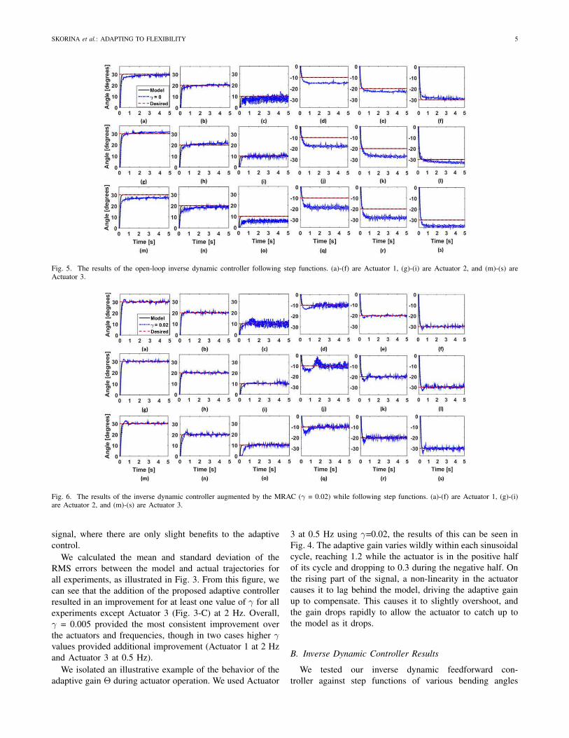
Fig. 7. The steady-state results of θ for the adaptive control augmentedinverse dynamic control.

[30◦, 20◦, 10◦,−10◦,−20◦, and −30◦] using each of thethree actuators. To show the advantages of the adaptivecontroller, we performed this experiment with and withoutadaptive control enabled (γ = 0.02). The higher γ was chosenbecause, for step references, rapid convergence is desired.We chose bm = 100 as it better matched the identifiedsystem model and the application meant we wouldn’t riska divergence of θ. In addition, we observed that using a ∆tof 0.001 in (9) would result in too much input saturation. Toprevent this, we used ∆t = 0.01 and replaced xm(n−1) withxm(n−10), making for a less exacting trajectory, inherentlyreducing the effect of any noise in sensor measurements. Theresults of this experiment without adaptation can be seen inFig. 5 while the results with adaptation can be seen in Fig. 6.

The inverse dynamic controller can quickly reach a desiredangle, even when operating without any feedback. However,it does result in some steady-state errors resulting from thedifferences between the reference model and the physicalsystem. The addition of the MRAC allowed the system tomaintain its fast approach while eliminating the steady-stateerror. We can also observe that the model and the plantbehave similarly during the approach to the desired angle,though the plant consistently overshoots before reacquiringthe target angle.

One thing we can observe from the non-adaptive tra-jectories is that the plant has a tendency to drift slowlyeven after the model input has stabilized. This representstime-variant dynamic behavior which has not been capturedby our model. Fortunately, the adaptive controller is ableto compensate for it. In addition, we can observe that thesteady-state error for the system varies widely with respectto the desired angle. The model actually gets more accurateat higher angles, and the errors are significantly differentbetween the positive and negative sides. This is becausethe characterization experiment used a constant input in thepositive direction that resulted in a large angle, so the modelis more accurate in these conditions.

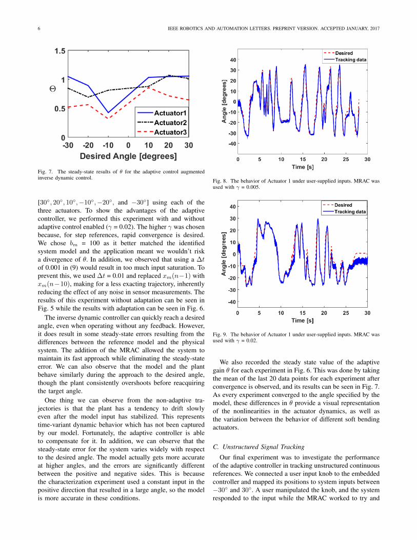
Fig. 8. The behavior of Actuator 1 under user-supplied inputs. MRAC wasused with γ = 0.005.

Fig. 9. The behavior of Actuator 1 under user-supplied inputs. MRAC wasused with γ = 0.02.

We also recorded the steady state value of the adaptivegain θ for each experiment in Fig. 6. This was done by takingthe mean of the last 20 data points for each experiment afterconvergence is observed, and its results can be seen in Fig. 7.As every experiment converged to the angle specified by themodel, these differences in θ provide a visual representationof the nonlinearities in the actuator dynamics, as well asthe variation between the behavior of different soft bendingactuators.

C. Unstructured Signal Tracking

Our final experiment was to investigate the performanceof the adaptive controller in tracking unstructured continuousreferences. We connected a user input knob to the embeddedcontroller and mapped its positions to system inputs between−30◦ and 30◦. A user manipulated the knob, and the systemresponded to the input while the MRAC worked to try and

SKORINA et al.: ADAPTING TO FLEXIBILITY 7

keep the system in sync with the model. Results of thesetrials can be seen in Fig. 8 with γ = 0.005 and Fig. 9 for γ= 0.02.

Results show that the model and the system behavesimilarly, even under the unstructured inputs. We can see theeffect of the lower γ, as in Fig. 8 the system does not respondfast enough to reach some of the peaks the model does.In addition, we can observe that the adaptive controller hasdifficulty matching the system to the model when the modelis around 0. This is because of the xm term in the adaptiveupdate equation in (5) indicates that when the model outputis near zero, θ will be updated slowly. Our control methodrequires the valves to be constantly operating, with an equal50% duty cycle for each valve supposedly correspondingto an angle of 0. Unfortunately, differences between ouractuators can cause this state to have a slight bias (for thisactuator, in the negative direction), something the MIT ruleadaptive MRAC is unable to compensate for.

VII. CONCLUSION

In this paper we formulated a model reference adaptivecontroller to ensure that our soft pneumatic bending actuatorsexhibit a behavior that is uniformly consistent with that ofa linear system model. We developed and characterized asimple linear dynamic model of our actuator, which served asa basis for our reference model. We applied our MRAC to arange of actuators under a range of frequencies and adaptiveupdate gains. We found that small update gains allowedfor increased performance in model following, while largergains would sometimes cause degradations in performance.In addition we used the dynamic actuator model to developa feed-forward inverse dynamic controller for our actuator toaugment the adaptive controller to ensure accurate positioncontrol of soft pneumatic actuators. We tested this controlleron different actuators against step functions of various am-plitudes and achieved successful tracking. Finally, we usedunstructured inputs from a user to provide reference positionsfor the actuator to track, demonstrating the versatility of theproposed control approach.

We observed that the adaptive gain θ converged to verydifferent results depending on where in the workspace thedesired position was located. In particular, it approacheddifferent values depending on if the actuator was bendingin positive or negative directions. This is likely the result ofdifferences between the two pressure chambers which weremolded separately and then attached together to form thefull actuator. When γ is high, it causes the actuator to overfit a single half-cycle, resulting in worse performance forthe other half-cycle. This is why increases in γ can cause adegradation in performance.

We would like to expand this work into a series ofactuators mounted together to form a soft pneumatic tentacle,each actuator running the same inverse-dynamic feedforwardaugmented MRAC. This approach will ensure that eachmodule behaves as desired, allowing the soft tentacle to

predictably perform manipulation tasks, such as squeezinginto tight spaces and grasping objects therein.

REFERENCES

[1] Y.-L. Park, S. J, G. K, E. C, Goldfield, and W. R.J, “A soft wearablerobotic device for active knee motions using flat pneumatic artificialmuscles,” in Robotics and Automation (ICRA), 2014 IEEE Interna-tional Conference on, pp. 4805–4810, IEEE, 2014.

[2] F. Renda, M. Cianchetti, M. Giorelli, A. Arienti, and C. Laschi, “A3d steady-state model of a tendon-driven continuum soft manipulatorinspired by the octopus arm,” Bioinspiration & biomimetics, vol. 7,no. 2, p. 025006, 2012.

[3] A. D. Marchese, C. D. Onal, and D. Rus, “Autonomous soft roboticfish capable of escape maneuvers using fluidic elastomer actuators,”Soft Robotics, vol. 1, no. 1, pp. 75–87, 2014.

[4] R. F. Shepherd, F. Ilievski, W. Choi, S. A. Morin, A. A. Stokes, A. D.Mazzeo, X. Chen, M. Wang, and G. M. Whitesides, “Multigait softrobot,” Proceedings of the National Academy of Sciences, vol. 108,no. 51, pp. 20400–20403, 2011.

[5] B. A. Trimmer, H.-T. Lin, A. Baryshyan, G. G. Leisk, and D. L.Kaplan, “Towards a biomorphic soft robot: design constraints andsolutions,” in 2012 4th IEEE RAS & EMBS International Conferenceon Biomedical Robotics and Biomechatronics (BioRob), pp. 599–605,IEEE, 2012.

[6] M. Luo, Y. Pan, E. Skorina, W. Tao, F. Chen, S. Ozel, and C. Onal,“Slithering towards autonomy: a self-contained soft robotic snake plat-form with integrated curvature sensing.,” Bioinspiration & biomimet-ics, vol. 10, no. 5, pp. 055001–055001, 2015.

[7] M. Luo, E. H. Skorina, W. Tao, F. Chen, S. Ozel, Y. Sun, and C. D.Onal, “Towards modular soft robotics: Proprioceptive curvature sens-ing and sliding-mode control of soft bidirectional bending modules,”Soft Robotics, 2016.

[8] B. Trimmer, “Soft robot control systems: A new grand challenge?,”Soft Robotics, vol. 1, 2014.

[9] J. C. Case, E. L. White, and R. K. Kramer, “Soft material characteri-zation for robotic applications,” Soft Robotics, vol. 2, no. 2, pp. 80–87,2015.

[10] Y. Sun, Y. S. Song, and J. Paik, “Characterization of silicone rubberbased soft pneumatic actuators,” in Intelligent Robots and Systems,2013. IEEE/RSJ International Conference on, pp. 4446–4453, IEEE,2013.

[11] H. Zhao, R. Huang, and R. F. Shepherd, “Curvature control of softorthotics via low cost solid-state optics,” in 2016 IEEE InternationalConference on Robotics and Automation (ICRA), pp. 4008–4013,IEEE, 2016.

[12] E. H. Skorina, M. Luo, S. Ozel, F. Chen, W. Tao, and C. D. Onal,“Feedforward augmented sliding mode motion control of antagonisticsoft pneumatic actuators,” in Robotics and Automation (ICRA), 2015IEEE International Conference on, pp. 2544–2549, IEEE, 2015.

[13] P. Polygerinos, Z. Wang, J. T. Overvelde, K. C. Galloway, R. J.Wood, K. Bertoldi, and C. J. Walsh, “Modeling of soft fiber-reinforcedbending actuators,” IEEE Transactions on Robotics, vol. 31, no. 3,pp. 778–789, 2015.

[14] N. Farrow and N. Correll, “A soft pneumatic actuator that can sensegrasp and touch,” in Intelligent Robots and Systems, 2015. IEEE/RSJInternational Conference on, pp. 2317–2323, IEEE, 2015.

[15] C. Onal and D. Rus, “Autonomous undulatory serpentine locomotionutilizing body dynamics of a fluidic soft robot,” Bioinspiration andBiomimetics, vol. 8, no. 2, 2013.

[16] C.-c. Hang and P. Parks, “Comparative studies of model referenceadaptive control systems,” IEEE transactions on automatic control,vol. 18, no. 5, pp. 419–428, 1973.

[17] G. Tonietti and A. Bicchi, “Adaptive simultaneous position and stiff-ness control for a soft robot arm,” in Intelligent Robots and Systems,2002 IEEE International Conference on, pp. 1992–1997, IEEE, 2002.

[18] S. Ozel, N. Keskin, D. Khea, and C. Onal, “A precise embedded cur-vature sensor module for soft-bodied robots,” Sensors and ActuatorsA: Physical, vol. 236, pp. 349–356, 2015.

[19] M. Luo, E. Skorina, W. OO, W. Tao, F. Chen, S. Youssefian, N. Rahbar,and C. Onal, “Reverse pneumatic artificial muscles (rpams): Modeling,integration, and control,” PLOS One, 2016 (under review).