IEEE PES Task Force on Benchmark Systems for Stability ...IEEE PES Task Force on Benchmark Systems...
48
IEEE PES Task Force on Benchmark Systems for Stability Controls Report on the 68-bus system (New England / New York Test System) Version 4.0 - June 20 th , 2014 Rodrigo A. Ramos, Roman Kuiava, Tatiane C. C. Fernandes, Liciane C. Pataca and Moussa R. Mansour The present report refers to a small-signal stability and study carried over the New England / New York Test System [1] using the ANAREDE/PacDyn/Anatem package from CEPEL [2]. This report has the objective to show how the simulation of this system must be done using this package. The obtained results are comparable (and exhibit a good match with respect to the electromechanical modes) with the ones provided via Matlab/Simulink [3]. To facilitate the comprehension, this report is divided in three sections (according to the software to be used): Load Flow (ANAREDE); Small-Signal Stability Assessment via Eigenvalue Calculation (PacDyn); Numerical Simulation of the Nonlinear Model (Anatem) 1. Load Flow The load flow of the 68-bus system was calculated using the ANAREDE software. Both the input file (for the correct initialization of the software) and the obtained results are given below in sections 1.1 and 1.2. 1.1 Input File To use the ANAREDE software, an input file was produced containing the data on the topology of the system. In this input file, presented in Appendix A (and also available for download at the website), loads were modeled as constant power elements. Furthermore, it is in the input file that the algorithm for load flow calculation is defined. In this case, Newton's method was chosen.
Transcript of IEEE PES Task Force on Benchmark Systems for Stability ...IEEE PES Task Force on Benchmark Systems...

IEEE PES Task Force on Benchmark Systems for Stability Controls
Report on the 68-bus system (New England / New York Test System)
Version 4.0 - June 20th, 2014
Rodrigo A. Ramos, Roman Kuiava, Tatiane C. C. Fernandes, Liciane C. Pataca
and Moussa R. Mansour
The present report refers to a small-signal stability and study carried over the New England
/ New York Test System [1] using the ANAREDE/PacDyn/Anatem package from CEPEL [2].
This report has the objective to show how the simulation of this system must be done using this
package. The obtained results are comparable (and exhibit a good match with respect to the
electromechanical modes) with the ones provided via Matlab/Simulink [3]. To facilitate the
comprehension, this report is divided in three sections (according to the software to be used):
� Load Flow (ANAREDE);
� Small-Signal Stability Assessment via Eigenvalue Calculation (PacDyn);
� Numerical Simulation of the Nonlinear Model (Anatem)
1. Load Flow
The load flow of the 68-bus system was calculated using the ANAREDE software. Both the
input file (for the correct initialization of the software) and the obtained results are given below
in sections 1.1 and 1.2.
1.1 Input File
To use the ANAREDE software, an input file was produced containing the data on the
topology of the system. In this input file, presented in Appendix A (and also available for
download at the website), loads were modeled as constant power elements. Furthermore, it is in
the input file that the algorithm for load flow calculation is defined. In this case, Newton's
method was chosen.
2 Report
68-bus system (New England / New York Test System)
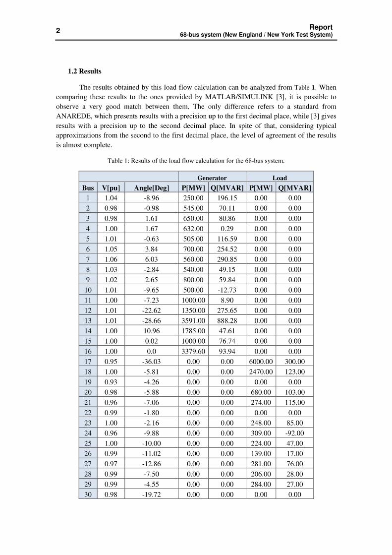
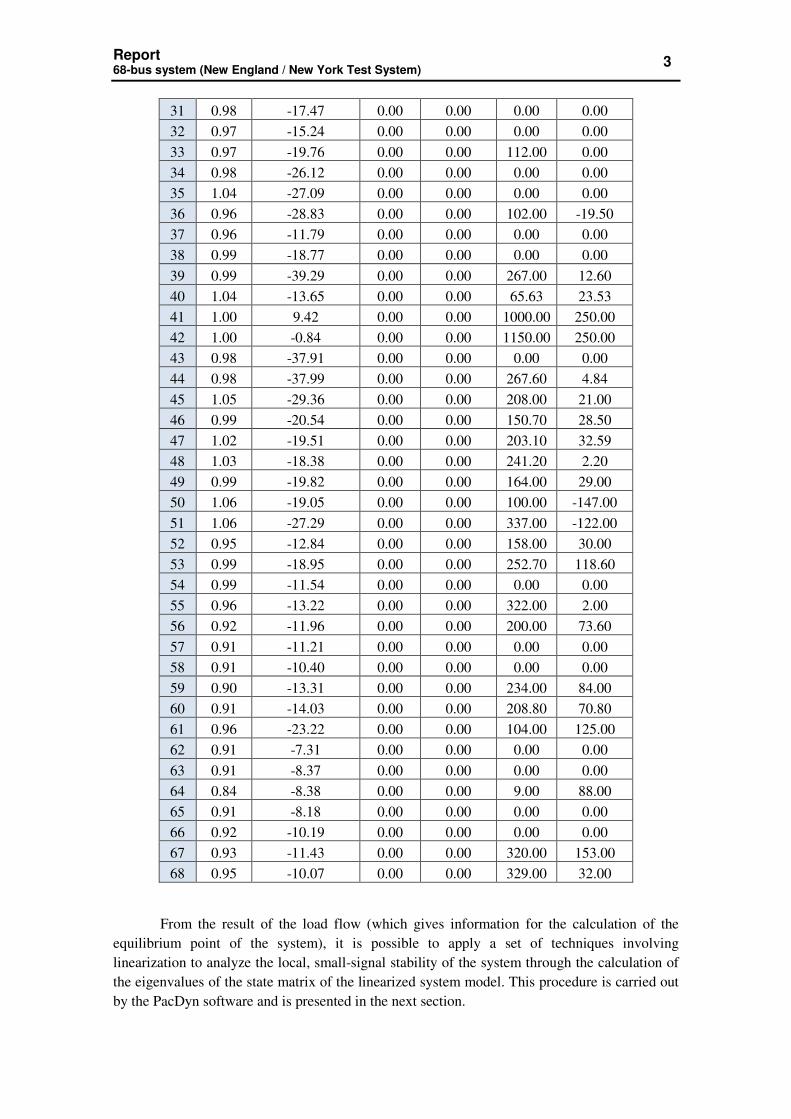
1.2 Results
The results obtained by this load flow calculation can be analyzed from Table 1. When
comparing these results to the ones provided by MATLAB/SIMULINK [3], it is possible to
observe a very good match between them. The only difference refers to a standard from
ANAREDE, which presents results with a precision up to the first decimal place, while [3] gives
results with a precision up to the second decimal place. In spite of that, considering typical
approximations from the second to the first decimal place, the level of agreement of the results
is almost complete.
Table 1: Results of the load flow calculation for the 68-bus system.
Generator Load
Bus V[pu] Angle[Deg] P[MW] Q[MVAR] P[MW] Q[MVAR] 1 1.04 -8.96 250.00 196.15 0.00 0.00
2 0.98 -0.98 545.00 70.11 0.00 0.00
3 0.98 1.61 650.00 80.86 0.00 0.00
4 1.00 1.67 632.00 0.29 0.00 0.00
5 1.01 -0.63 505.00 116.59 0.00 0.00
6 1.05 3.84 700.00 254.52 0.00 0.00
7 1.06 6.03 560.00 290.85 0.00 0.00
8 1.03 -2.84 540.00 49.15 0.00 0.00
9 1.02 2.65 800.00 59.84 0.00 0.00
10 1.01 -9.65 500.00 -12.73 0.00 0.00
11 1.00 -7.23 1000.00 8.90 0.00 0.00
12 1.01 -22.62 1350.00 275.65 0.00 0.00
13 1.01 -28.66 3591.00 888.28 0.00 0.00
14 1.00 10.96 1785.00 47.61 0.00 0.00
15 1.00 0.02 1000.00 76.74 0.00 0.00
16 1.00 0.0 3379.60 93.94 0.00 0.00
17 0.95 -36.03 0.00 0.00 6000.00 300.00
18 1.00 -5.81 0.00 0.00 2470.00 123.00
19 0.93 -4.26 0.00 0.00 0.00 0.00
20 0.98 -5.88 0.00 0.00 680.00 103.00
21 0.96 -7.06 0.00 0.00 274.00 115.00
22 0.99 -1.80 0.00 0.00 0.00 0.00
23 1.00 -2.16 0.00 0.00 248.00 85.00
24 0.96 -9.88 0.00 0.00 309.00 -92.00
25 1.00 -10.00 0.00 0.00 224.00 47.00
26 0.99 -11.02 0.00 0.00 139.00 17.00
27 0.97 -12.86 0.00 0.00 281.00 76.00
28 0.99 -7.50 0.00 0.00 206.00 28.00
29 0.99 -4.55 0.00 0.00 284.00 27.00
30 0.98 -19.72 0.00 0.00 0.00 0.00
Report 68-bus system (New England / New York Test System)
3
31 0.98 -17.47 0.00 0.00 0.00 0.00
32 0.97 -15.24 0.00 0.00 0.00 0.00
33 0.97 -19.76 0.00 0.00 112.00 0.00
34 0.98 -26.12 0.00 0.00 0.00 0.00
35 1.04 -27.09 0.00 0.00 0.00 0.00
36 0.96 -28.83 0.00 0.00 102.00 -19.50
37 0.96 -11.79 0.00 0.00 0.00 0.00
38 0.99 -18.77 0.00 0.00 0.00 0.00
39 0.99 -39.29 0.00 0.00 267.00 12.60
40 1.04 -13.65 0.00 0.00 65.63 23.53
41 1.00 9.42 0.00 0.00 1000.00 250.00
42 1.00 -0.84 0.00 0.00 1150.00 250.00
43 0.98 -37.91 0.00 0.00 0.00 0.00
44 0.98 -37.99 0.00 0.00 267.60 4.84
45 1.05 -29.36 0.00 0.00 208.00 21.00
46 0.99 -20.54 0.00 0.00 150.70 28.50
47 1.02 -19.51 0.00 0.00 203.10 32.59
48 1.03 -18.38 0.00 0.00 241.20 2.20
49 0.99 -19.82 0.00 0.00 164.00 29.00
50 1.06 -19.05 0.00 0.00 100.00 -147.00
51 1.06 -27.29 0.00 0.00 337.00 -122.00
52 0.95 -12.84 0.00 0.00 158.00 30.00
53 0.99 -18.95 0.00 0.00 252.70 118.60
54 0.99 -11.54 0.00 0.00 0.00 0.00
55 0.96 -13.22 0.00 0.00 322.00 2.00
56 0.92 -11.96 0.00 0.00 200.00 73.60
57 0.91 -11.21 0.00 0.00 0.00 0.00
58 0.91 -10.40 0.00 0.00 0.00 0.00
59 0.90 -13.31 0.00 0.00 234.00 84.00
60 0.91 -14.03 0.00 0.00 208.80 70.80
61 0.96 -23.22 0.00 0.00 104.00 125.00
62 0.91 -7.31 0.00 0.00 0.00 0.00
63 0.91 -8.37 0.00 0.00 0.00 0.00
64 0.84 -8.38 0.00 0.00 9.00 88.00
65 0.91 -8.18 0.00 0.00 0.00 0.00
66 0.92 -10.19 0.00 0.00 0.00 0.00
67 0.93 -11.43 0.00 0.00 320.00 153.00
68 0.95 -10.07 0.00 0.00 329.00 32.00
From the result of the load flow (which gives information for the calculation of the
equilibrium point of the system), it is possible to apply a set of techniques involving
linearization to analyze the local, small-signal stability of the system through the calculation of
the eigenvalues of the state matrix of the linearized system model. This procedure is carried out
by the PacDyn software and is presented in the next section.
4 Report
68-bus system (New England / New York Test System)
2. Small-Signal Stability Analysis of the System
To use the PacDyn software for assessment of the small-signal stability of the 68-bus
system, two input files are necessary. One of them contains the topological data of the system
and the results of the load flow calculation, while the other contains the types of models, the
structures and the parameters of the generators and its associated controllers. The former is
obtained as an output file from the ANAREDE software in the “*.his” or “*.sav” formats. The
latter, containing the dynamic data for the system, must be constructed and saved in the “*.dyn”
format. This format is described in more detail in section 2.1, while section 2.2 presents the
results of the whole study.
2.1 The input file with the dynamic data for the system
In the input file containing the dynamic data for the system (the “*.dyn” file) the models to
represent the generators in the system must be chosen, and the controllers for each respective
machine must be either chosen as built-in models or defined by the user with a particular syntax.
For this study, the details on the model of the generators and its respective controllers are
presented in the sequence:
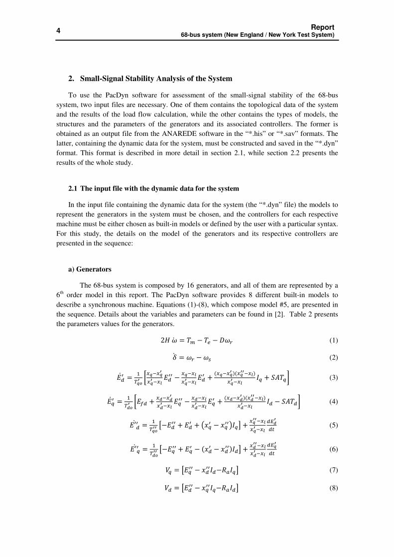
a) Generators
The 68-bus system is composed by 16 generators, and all of them are represented by a
6th order model in this report. The PacDyn software provides 8 different built-in models to
describe a synchronous machine. Equations (1)-(8), which compose model #5, are presented in
the sequence. Details about the variables and parameters can be found in [2]. Table 2 presents
the parameters values for the generators.
2��� = �� − � − ��� (1)
� = �� −�� (2)
���� = ����� ������������� ��
�� − �������������
� + (������ )(�������)������ �� + !��" (3)
���� = ��#�� ��$� + �#��#�
�#�������� − �#���
�#������� + (�#��#� )(�#�����)
�#������ − !��" (4)
�′��� = ������ &−��
�� + ��� + '(�� − (���)��* + �������������
�+#��, (5)
�′��� = ��#��� &−��
�� + ��� − ((�� − (���)��* + �#������#����
�+���, (6)
-� = &���� − (�����−./��* (7)
-� = &���� − (�����−./��* (8)

Report 68-bus system (New England / New York Test System)
5
Table 2: Generator parameters.
Unit H Ra x''d x''q x'd x'q xd xq xl T’’do T’’qo T’do T’qo
1 42.0 0 0.025 0.025 0.031 0.0417 0.10 0.069 0.0125 0.05 0.035 10.2 1.5
2 30.2 0 0.050 0.050 0.0697 0.0933 0.295 0.282 0.035 0.05 0.035 6.56 1.5
3 35.8 0 0.045 0.045 0.0531 0.0714 0.2495 0.237 0.0304 0.05 0.035 5.7 1.5
4 28.6 0 0.035 0.035 0.0436 0.0586 0.262 0.258 0.0295 0.05 0.035 5.69 1.5
5 26.0 0 0.050 0.050 0.066 0.0883 0.330 0.310 0.027 0.05 0.035 5.4 0.44
6 34.8 0 0.040 0.040 0.050 0.0675 0.254 0.241 0.0224 0.05 0.035 7.3 0.4
7 26.4 0 0.040 0.040 0.049 0.0667 0.295 0.292 0.0322 0.05 0.035 5.66 1.5
8 24.3 0 0.045 0.045 0.057 0.0767 0.290 0.280 0.028 0.05 0.035 6.7 0.41
9 34.5 0 0.045 0.045 0.057 0.0767 0.2106 0.205 0.0298 0.05 0.035 4.79 1.96
10 31.0 0 0.040 0.040 0.0457 0.0615 0.169 0.115 0.0199 0.05 0.035 9.37 1.5
11 28.2 0 0.012 0.012 0.018 0.0241 0.128 0.123 0.0103 0.05 0.035 4.1 1.5
12 92.3 0 0.025 0.025 0.031 0.0420 0.101 0.095 0.022 0.05 0.035 7.4 1.5
13 248.0 0 0.004 0.004 0.0055 0.0074 0.0296 0.0286 0.003 0.05 0.035 5.9 1.5
14 300.0 0 0.0023 0.0023 0.0029 0.0038 0.018 0.0173 0.0017 0.05 0.035 4.1 1.5
15 300.0 0 0.0023 0.0023 0.0029 0.0038 0.018 0.0173 0.0017 0.05 0.035 4.1 1.5
16 225.0 0 0.0055 0.0055 0.0071 0.0095 0.0356 0.0334 0.0041 0.05 0.035 7.8 1.5
Unit D MVA base
1 0 100
2 0 100
3 0 100
4 0 100
5 0 100
6 0 100
7 0 100
8 0 100
9 0 100
10 0 100
11 0 100
12 0 100
13 0 200
14 0 100
15 0 100
16 0 200
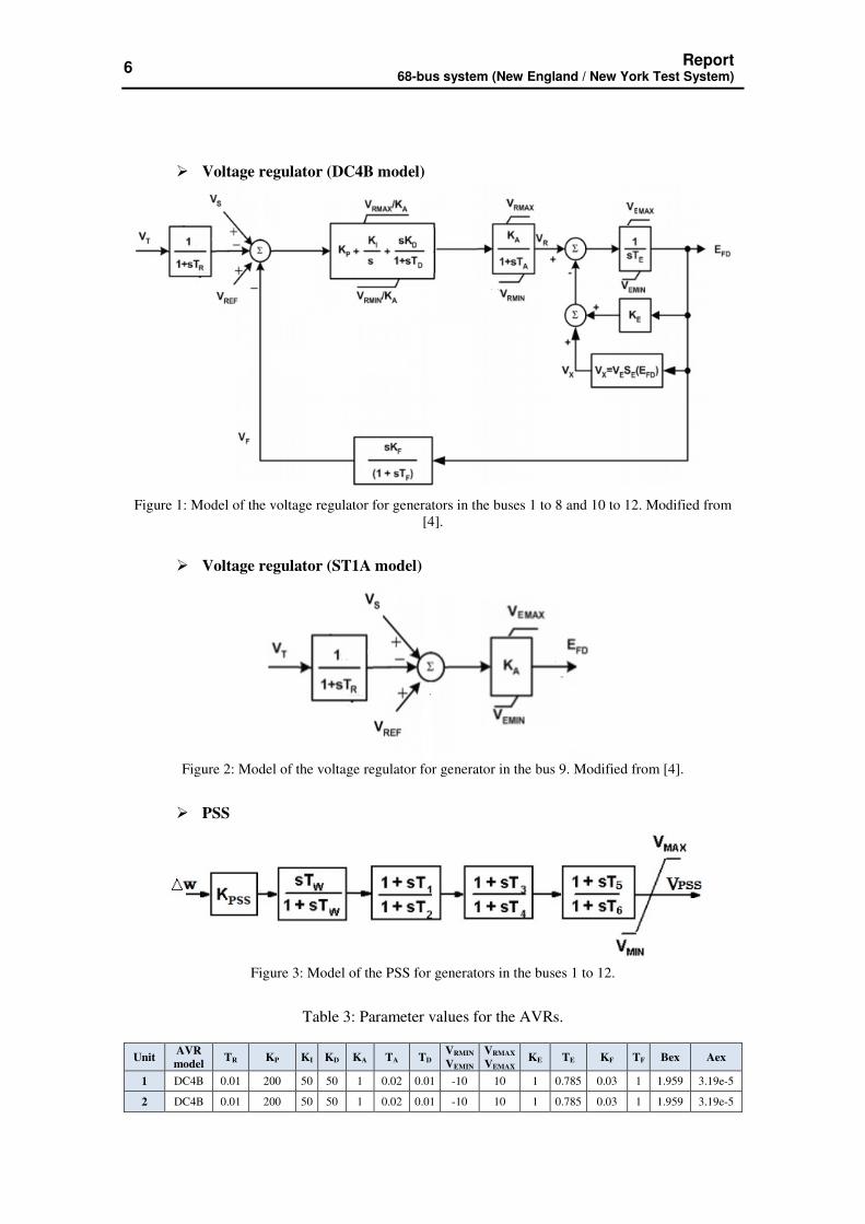
b) Controllers
The generators in the buses 1 to 12 in this system are equipped with automatic voltage
regulators (AVRs) and power system stabilizers (PSSs). The generators in buses 1 to 8 and 10 to
12 use the AVR-DC4B model [5] with same parameter values and the generator in bus 9 use the
AVR-STA1 model [4]. For the records, the block diagram of each controller model is presented
as follows in Figures 1 and 2. Tables 3 and 4 present the parameter values for the AVRs and
PSS, respectively.
6 Report
68-bus system (New England / New York Test System)
� Voltage regulator (DC4B model)
Figure 1: Model of the voltage regulator for generators in the buses 1 to 8 and 10 to 12. Modified from
[4].
� Voltage regulator (ST1A model)
Figure 2: Model of the voltage regulator for generator in the bus 9. Modified from [4].
� PSS
Figure 3: Model of the PSS for generators in the buses 1 to 12.
Table 3: Parameter values for the AVRs.
Unit AVR model
TR KP KI KD KA TA TD VRMIN
VEMIN
VRMAX
VEMAX KE TE KF TF Bex Aex
1 DC4B 0.01 200 50 50 1 0.02 0.01 -10 10 1 0.785 0.03 1 1.959 3.19e-5
2 DC4B 0.01 200 50 50 1 0.02 0.01 -10 10 1 0.785 0.03 1 1.959 3.19e-5

Report 68-bus system (New England / New York Test System)
7
3 DC4B 0.01 200 50 50 1 0.02 0.01 -10 10 1 0.785 0.03 1 1.959 3.19e-5
4 DC4B 0.01 200 50 50 1 0.02 0.01 -10 10 1 0.785 0.03 1 1.959 3.19e-5
5 DC4B 0.01 200 50 50 1 0.02 0.01 -10 10 1 0.785 0.03 1 1.959 3.19e-5
6 DC4B 0.01 200 50 50 1 0.02 0.01 -10 10 1 0.785 0.03 1 1.959 3.19e-5
7 DC4B 0.01 200 50 50 1 0.02 0.01 -10 10 1 0.785 0.03 1 1.959 3.19e-5
8 DC4B 0.01 200 50 50 1 0.02 0.01 -10 10 1 0.785 0.03 1 1.959 3.19e-5
9 ST1A 0.01 --- --- --- 200 --- --- -5 5 --- --- --- --- --- ---
10 DC4B 0.01 200 50 50 1 0.02 0.01 -10 10 1 0.785 0.03 1 1.959 3.19e-5
11 DC4B 0.01 200 50 50 1 0.02 0.01 -10 10 1 0.785 0.03 1 1.959 3.19e-5
12 DC4B 0.01 200 50 50 1 0.02 0.01 -10 10 1 0.785 0.03 1 1.959 3.19e-5
Table 4: Parameter values for the PSSs connected to generators in buses 1 to 12.
Unit KPSS Tw T1 T2 T3 T4 T5 T6 VMIN VMÁX
1 20 15 0.15 0.04 0.15 0.04 0.15 0.04 -0.05 0.2
2 20 15 0.15 0.04 0.15 0.04 0.15 0.04 -0.05 0.2
3 20 15 0.15 0.04 0.15 0.04 0.15 0.04 -0.05 0.2
4 20 15 0.15 0.04 0.15 0.04 0.15 0.04 -0.05 0.2
5 20 15 0.15 0.04 0.15 0.04 0.15 0.04 -0.05 0.2
6 20 15 0.15 0.04 0.15 0.04 0.15 0.04 -0.05 0.2
7 20 15 0.15 0.04 0.15 0.04 0.15 0.04 -0.05 0.2
8 20 15 0.15 0.04 0.15 0.04 0.15 0.04 -0.05 0.2
9 12 10 0.09 0.02 0.09 0.02 0 0 -0.05 0.2
10 20 15 0.15 0.04 0.15 0.04 0.15 0.04 -0.05 0.2
11 20 15 0.15 0.04 0.15 0.04 0.15 0.04 -0.05 0.2
12 20 15 0.15 0.04 0.15 0.04 0.15 0.04 -0.05 0.2
2.2 Results
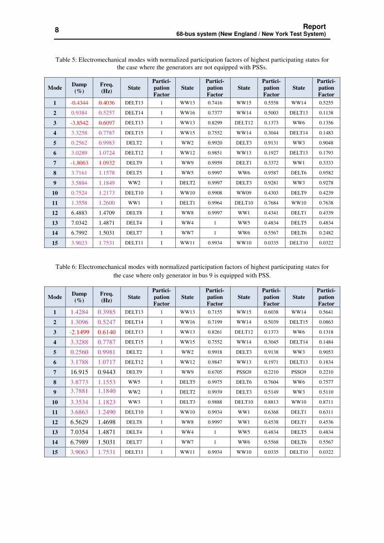
The results obtained by PacDyn on the small-signal stability analysis of the 68-bus
system can be seen in Tables 5, 6 and 7. These results are comparable with the ones calculated
via MATLAB/SIMULINK [3], as it can be seen in Figures 4, 5 and 6. Table 5 shows the
electromechanical modes with normalized participation factors of highest participating states for
the case where the generators are not equipped with PSSs. It can be seen that three modes are
unstable and others 9 modes are poorly damped (considering a minimum acceptable damping of
5%).
8 Report
68-bus system (New England / New York Test System)
Table 5: Electromechanical modes with normalized participation factors of highest participating states for
the case where the generators are not equipped with PSSs.
Mode Damp (%)
Freq. (Hz)
State Partici-pation Factor
State Partici- pation Factor
State Partici- pation Factor
State Partici- pation Factor
1 -0.4344 0.4036 DELT13 1 WW13 0.7416 WW15 0.5558 WW14 0.5255
2 0.9384 0.5257 DELT14 1 WW16 0.7377 WW14 0.5003 DELT13 0.1138
3 -3.8542 0.6097 DELT13 1 WW13 0.8299 DELT12 0.1373 WW6 0.1356
4 3.3258 0.7787 DELT15 1 WW15 0.7552 WW14 0.3044 DELT14 0.1483
5 0.2562 0.9983 DELT2 1 WW2 0.9920 DELT3 0.9131 WW3 0.9048
6 3.0289 1.0724 DELT12 1 WW12 0.9851 WW13 0.1927 DELT13 0.1793
7 -1.8063 1.0932 DELT9 1 WW9 0.9959 DELT1 0.3372 WW1 0.3333
8 3.7161 1.1578 DELT5 1 WW5 0.9997 WW6 0.9587 DELT6 0.9582
9 3.5884 1.1849 WW2 1 DELT2 0.9997 DELT3 0.9281 WW3 0.9278
10 0.7524 1.2173 DELT10 1 WW10 0.9908 WW09 0.4303 DELT9 0.4239
11 1.3558 1.2600 WW1 1 DELT1 0.9964 DELT10 0.7684 WW10 0.7638
12 6.4883 1.4709 DELT8 1 WW8 0.9997 WW1 0.4341 DELT1 0.4339
13 7.0342 1.4871 DELT4 1 WW4 1 WW5 0.4834 DELT5 0.4834
14 6.7992 1.5031 DELT7 1 WW7 1 WW6 0.5567 DELT6 0.2482
15 3.9023 1.7531 DELT11 1 WW11 0.9934 WW10 0.0335 DELT10 0.0322
Table 6: Electromechanical modes with normalized participation factors of highest participating states for
the case where only generator in bus 9 is equipped with PSS.
Mode Damp (%)
Freq. (Hz)
State Partici-pation Factor
State Partici- pation Factor
State Partici- pation Factor
State Partici- pation Factor
1 1.4284 0.3985 DELT13 1 WW13 0.7155 WW15 0.6038 WW14 0.5641
2 1.3096 0.5247 DELT14 1 WW16 0.7199 WW14 0.5039 DELT15 0.0863
3 -2.1499 0.6140 DELT13 1 WW13 0.8261 DELT12 0.1373 WW6 0.1318
4 3.3288 0.7787 DELT15 1 WW15 0.7552 WW14 0.3045 DELT14 0.1484
5 0.2560 0.9981 DELT2 1 WW2 0.9918 DELT3 0.9138 WW3 0.9053
6 3.1788 1.0717 DELT12 1 WW12 0.9847 WW13 0.1971 DELT13 0.1834
7 16.915 0.9443 DELT9 1 WW9 0.6705 PSSG9 0.2210 PSSG9 0.2210
8 3.8773 1.1553 WW5 1 DELT5 0.9975 DELT6 0.7604 WW6 0.7577
9 3.7881 1.1840 WW2 1 DELT2 0.9939 DELT3 0.5149 WW3 0.5110
10 3.3534 1.1823 WW3 1 DELT3 0.9888 DELT10 0.8813 WW10 0.8711
11 3.6863 1.2490 DELT10 1 WW10 0.9934 WW1 0.6368 DELT1 0.6311
12 6.5629 1.4698 DELT8 1 WW8 0.9997 WW1 0.4538 DELT1 0.4536
13 7.0354 1.4871 DELT4 1 WW4 1 WW5 0.4834 DELT5 0.4834
14 6.7989 1.5031 DELT7 1 WW7 1 WW6 0.5568 DELT6 0.5567
15 3.9063 1.7531 DELT11 1 WW11 0.9934 WW10 0.0335 DELT10 0.0322
Report 68-bus system (New England / New York Test System
Table 7: Electromechanical modes
Mode
1
2
3
4
5
6
7
8
Figure 4: Eigenvalues (calculated from MATLAB/SIMULINK [3] and PacDyn) for the case where the
Figure 5: Eigenvalues (calculated from MATLAB/SIMULINK [3] and PacDyn) for the case where only
/ New York Test System)
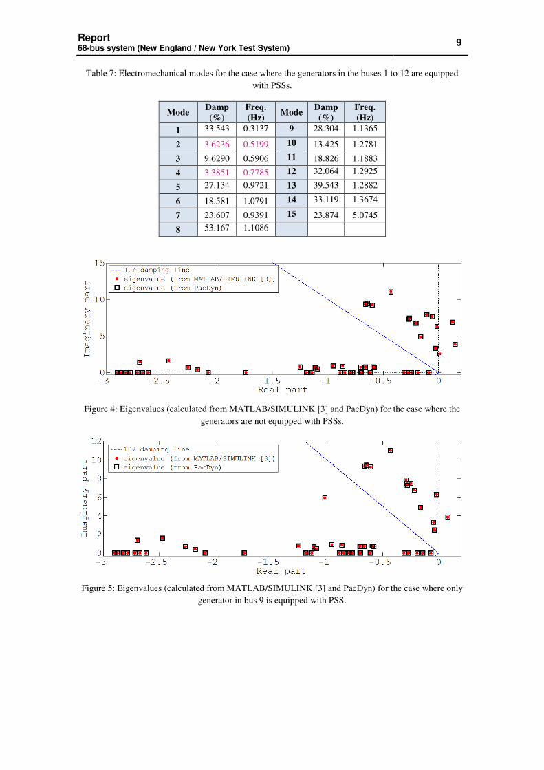
lectromechanical modes for the case where the generators in the buses 1 to 12 are equipped
with PSSs.
Damp (%)
Freq. (Hz)
Mode Damp (%)
Freq. (Hz)
33.543 0.3137 9 28.304 1.1365
3.6236 0.5199 10 13.425 1.2781
9.6290 0.5906 11 18.826 1.1883
3.3851 0.7785 12 32.064 1.2925
27.134 0.9721 13 39.543 1.2882
18.581 1.0791 14 33.119 1.3674
23.607 0.9391 15 23.874 5.0745
53.167 1.1086
Figure 4: Eigenvalues (calculated from MATLAB/SIMULINK [3] and PacDyn) for the case where the
generators are not equipped with PSSs.
Figure 5: Eigenvalues (calculated from MATLAB/SIMULINK [3] and PacDyn) for the case where only
generator in bus 9 is equipped with PSS.
9
for the case where the generators in the buses 1 to 12 are equipped
Figure 4: Eigenvalues (calculated from MATLAB/SIMULINK [3] and PacDyn) for the case where the
Figure 5: Eigenvalues (calculated from MATLAB/SIMULINK [3] and PacDyn) for the case where only
10
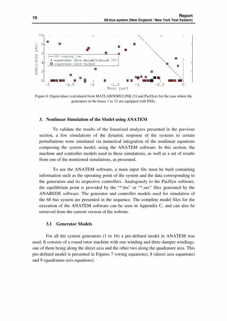
Figure 6: Eigenvalues (calculated from MATLAB/SIMULINK [3] and PacDyn) for the case where the
generators in the buses
3. Nonlinear Simulation of the Model using ANATEM
To validate the results of the linearized analyzes presented in the previous
section, a few simulations of the dynamic response of the systems to certain
perturbations were simulated via numerical integration of the nonlinear equations
composing the system model, using the ANATEM software. In this section, the
machine and controller models used in these simulations, as well as a set of results
from one of the mentioned simula
To use the ANATEM software, a main input file must be built containing
information such as the operating point of the system and the data corresponding to
the generators and its respective controllers. Analogously to the PacDyn softwar
the equilibrium point is provided by the “*.his” or “*.sav” files generated by the
ANAREDE software. The generator and controller models used for simulation of
the 68 bus system are presented in the sequence. The complete model files for the
execution of the ANATEM software can be seen in Appendix
retrieved from the current version of the website.
3.1 Generator Models
For all the system generators (1 to 16) a pre
used. It consists of a round rotor
one of them being along the direct axis and the other two along the quadrature axis. This
pre-defined model is presented in Figures 7 (swing equations), 8 (direct axis equations)
and 9 (quadrature axis equations).
68-bus system (New England / New York Test System
Figure 6: Eigenvalues (calculated from MATLAB/SIMULINK [3] and PacDyn) for the case where the
generators in the buses 1 to 12 are equipped with PSSs.
Simulation of the Model using ANATEM
To validate the results of the linearized analyzes presented in the previous
section, a few simulations of the dynamic response of the systems to certain
simulated via numerical integration of the nonlinear equations
composing the system model, using the ANATEM software. In this section, the
machine and controller models used in these simulations, as well as a set of results
from one of the mentioned simulations, as presented.
To use the ANATEM software, a main input file must be built containing
information such as the operating point of the system and the data corresponding to
the generators and its respective controllers. Analogously to the PacDyn softwar
the equilibrium point is provided by the “*.his” or “*.sav” files generated by the
ANAREDE software. The generator and controller models used for simulation of
the 68 bus system are presented in the sequence. The complete model files for the
f the ANATEM software can be seen in Appendix C, and can also be
retrieved from the current version of the website.
Generator Models
For all the system generators (1 to 16) a pre-defined model in ANATEM was
used. It consists of a round rotor machine with one winding and three damper windings
one of them being along the direct axis and the other two along the quadrature axis. This
defined model is presented in Figures 7 (swing equations), 8 (direct axis equations)
uations).
Report / New York Test System)
Figure 6: Eigenvalues (calculated from MATLAB/SIMULINK [3] and PacDyn) for the case where the
To validate the results of the linearized analyzes presented in the previous
section, a few simulations of the dynamic response of the systems to certain
simulated via numerical integration of the nonlinear equations
composing the system model, using the ANATEM software. In this section, the
machine and controller models used in these simulations, as well as a set of results
To use the ANATEM software, a main input file must be built containing
information such as the operating point of the system and the data corresponding to
the generators and its respective controllers. Analogously to the PacDyn software,
the equilibrium point is provided by the “*.his” or “*.sav” files generated by the
ANAREDE software. The generator and controller models used for simulation of
the 68 bus system are presented in the sequence. The complete model files for the
, and can also be
defined model in ANATEM was
machine with one winding and three damper windings,
one of them being along the direct axis and the other two along the quadrature axis. This
defined model is presented in Figures 7 (swing equations), 8 (direct axis equations)

Report 68-bus system (New England / New York Test System)
11
Figure 7: Block diagram for the swing equation of the model for generators 1 to 16.
Figure 8: Block diagram for the direct axis equations of the model for generators 1 to
16.

12 Report
68-bus system (New England / New York Test System)
Figure 9: Block diagram for the quadrature axis equations of the model for generators 1
to 16.
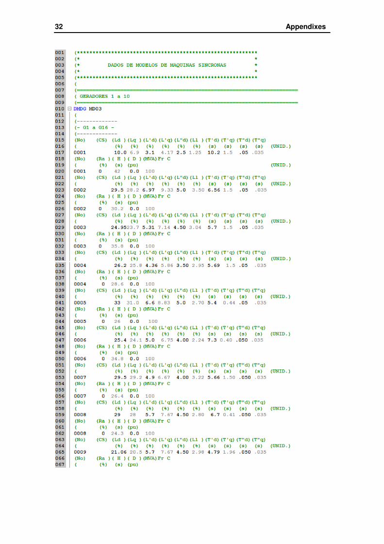
In this simulation the saturation curves of the generators were not represented.
The parameters used for these models are presented in Table 2. The synchronous
machine models are provided within the file 16GENERATOR.blt, presented in
Appendix C and available for download at the website.
3.2 Controller Models
The controller models were defined by the users via the execution code DCDU
and are given in the file 16GENERATOR.cdu, also presented in Appendix C. These
models and its parameters were also retrieved from the website, and were already
presented in Figures 1, 2 and 3 of this report.
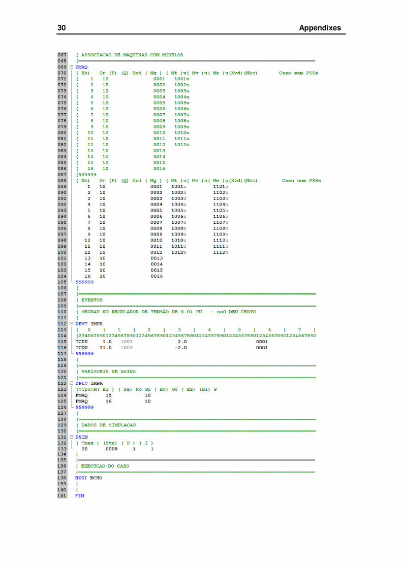
3.3 Results a) Perturbation Data In the nonlinear simulations using ANATEM, two cases were considered (and
compared with nonlinear simulation obtained from MATLAB/SIMULINK [3]):
i) A 20s simulation with a 2% step in Vref of the test machine at t=1.0s and
a -2% step in the same Vref at t=11s.
ii) The connection at t=1.0s of a 50MVAr shunt reactor to the bus 3,
removing this reactor at t=11s and simulating until t=20s.
Report 68-bus system (New England / New York Test System)
13
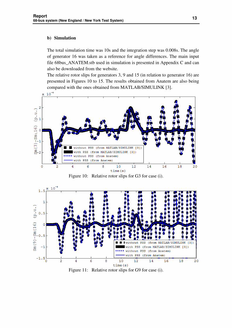
b) Simulation
The total simulation time was 10s and the integration step was 0.008s. The angle
of generator 16 was taken as a reference for angle differences. The main input
file 68bus_ANATEM.stb used in simulation is presented in Appendix C and can
also be downloaded from the website.
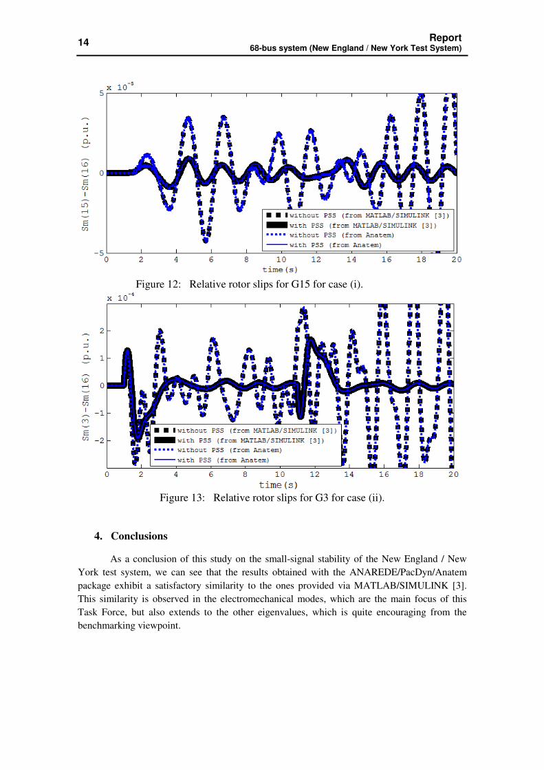
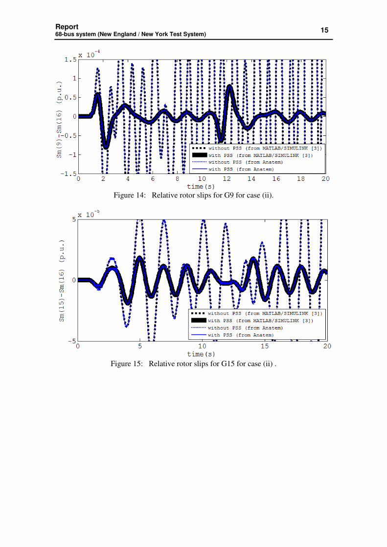
The relative rotor slips for generators 3, 9 and 15 (in relation to generator 16) are
presented in Figures 10 to 15. The results obtained from Anatem are also being
compared with the ones obtained from MATLAB/SIMULINK [3].
Figure 10: Relative rotor slips for G3 for case (i).
Figure 11: Relative rotor slips for G9 for case (i).
14 Report
68-bus system (New England / New York Test System)
Figure 12: Relative rotor slips for G15 for case (i).
Figure 13: Relative rotor slips for G3 for case (ii).
4. Conclusions
As a conclusion of this study on the small-signal stability of the New England / New
York test system, we can see that the results obtained with the ANAREDE/PacDyn/Anatem
package exhibit a satisfactory similarity to the ones provided via MATLAB/SIMULINK [3].
This similarity is observed in the electromechanical modes, which are the main focus of this
Task Force, but also extends to the other eigenvalues, which is quite encouraging from the
benchmarking viewpoint.
Report 68-bus system (New England / New York Test System)
15
Figure 14: Relative rotor slips for G9 for case (ii).
Figure 15: Relative rotor slips for G15 for case (ii) .

16 Report
68-bus system (New England / New York Test System)
Appendix A
In this appendix, the input file necessary for the correct initialization of the ANAREDE
software is presented. Figure A-1 shows how the bus data must be inserted while Figure A-2
performs a similar task with respect to the line data.
Continue in next page …

Report 68-bus system (New England / New York Test System)
17
Figure A-1: Input file for entering the bus data.
Continue in next page …
18 Report
68-bus system (New England / New York Test System)
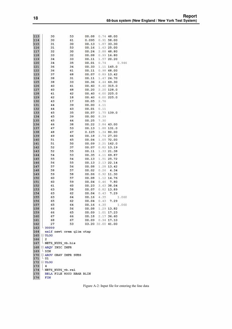
Figure A-2: Input file for entering the line data
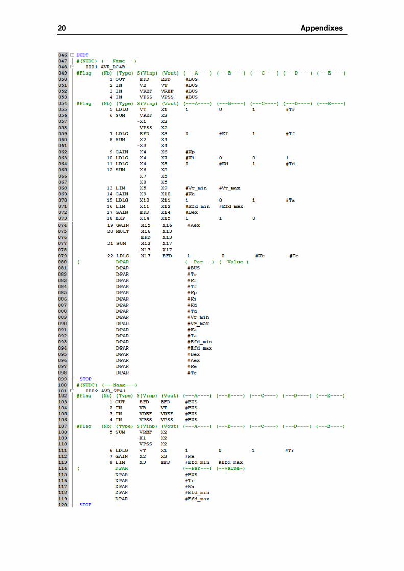
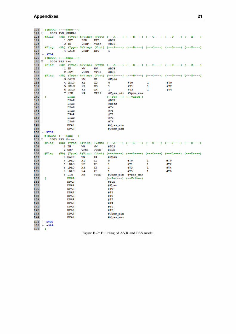
Appendix B
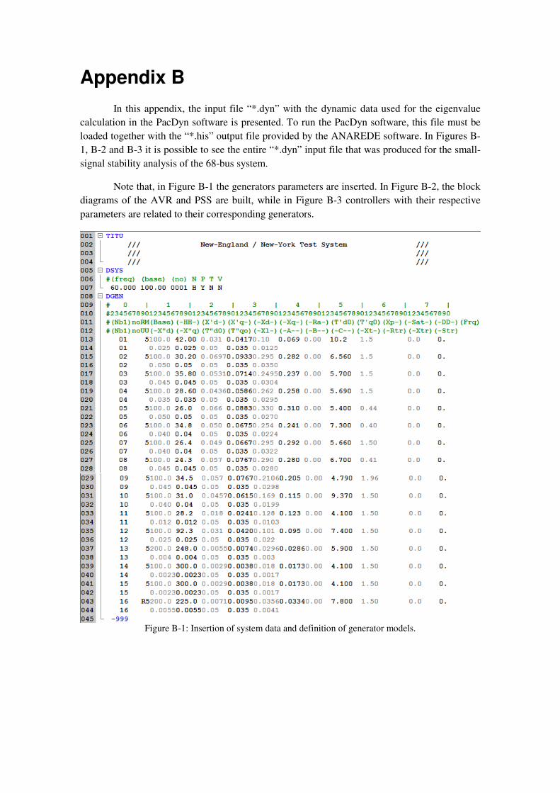
In this appendix, the input file “*.dyn” with the dynamic data used for the eigenvalue
calculation in the PacDyn software is presented. To run the PacDyn software, this file must be
loaded together with the “*.his” output file provided by the ANAREDE software. In Figures B-
1, B-2 and B-3 it is possible to see the entire “*.dyn” input file that was produced for the small-
signal stability analysis of the 68-bus system.
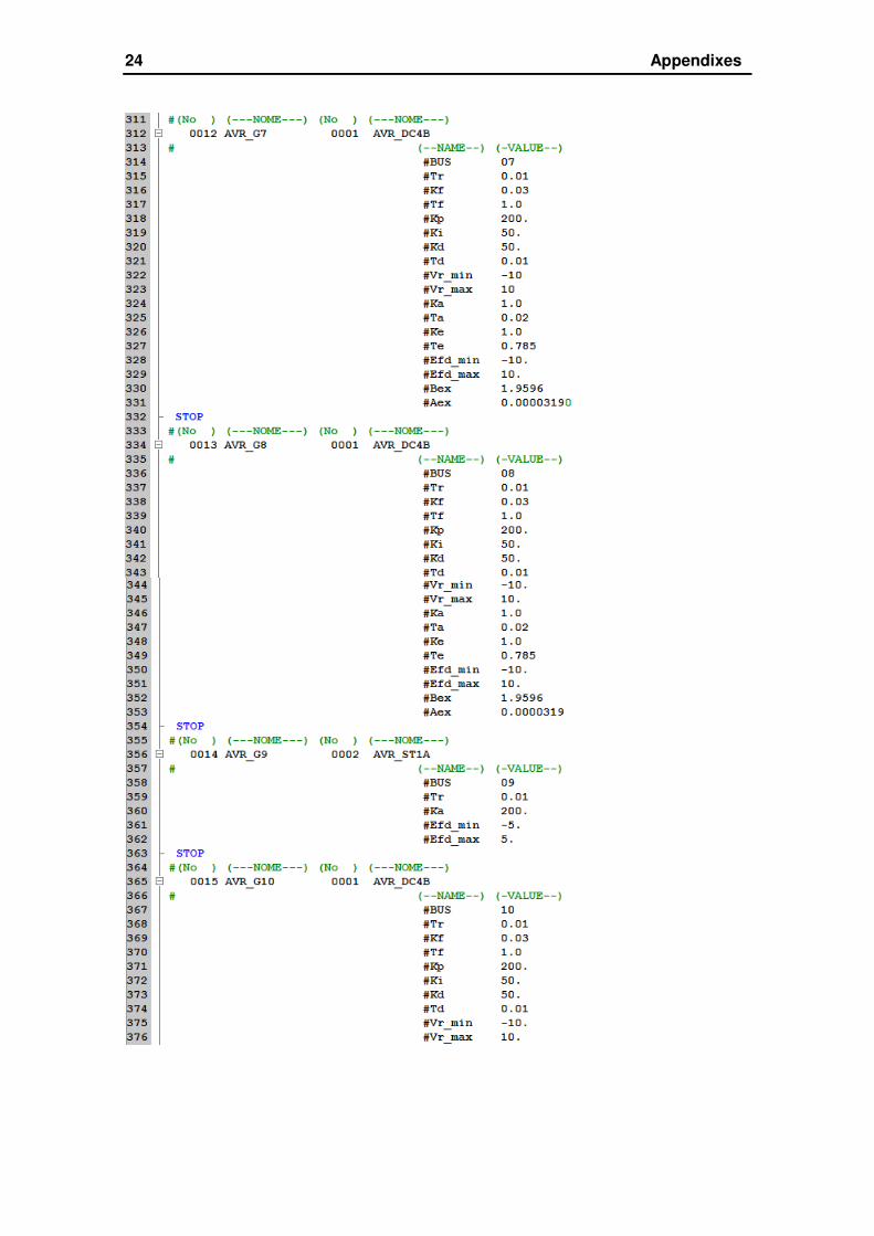
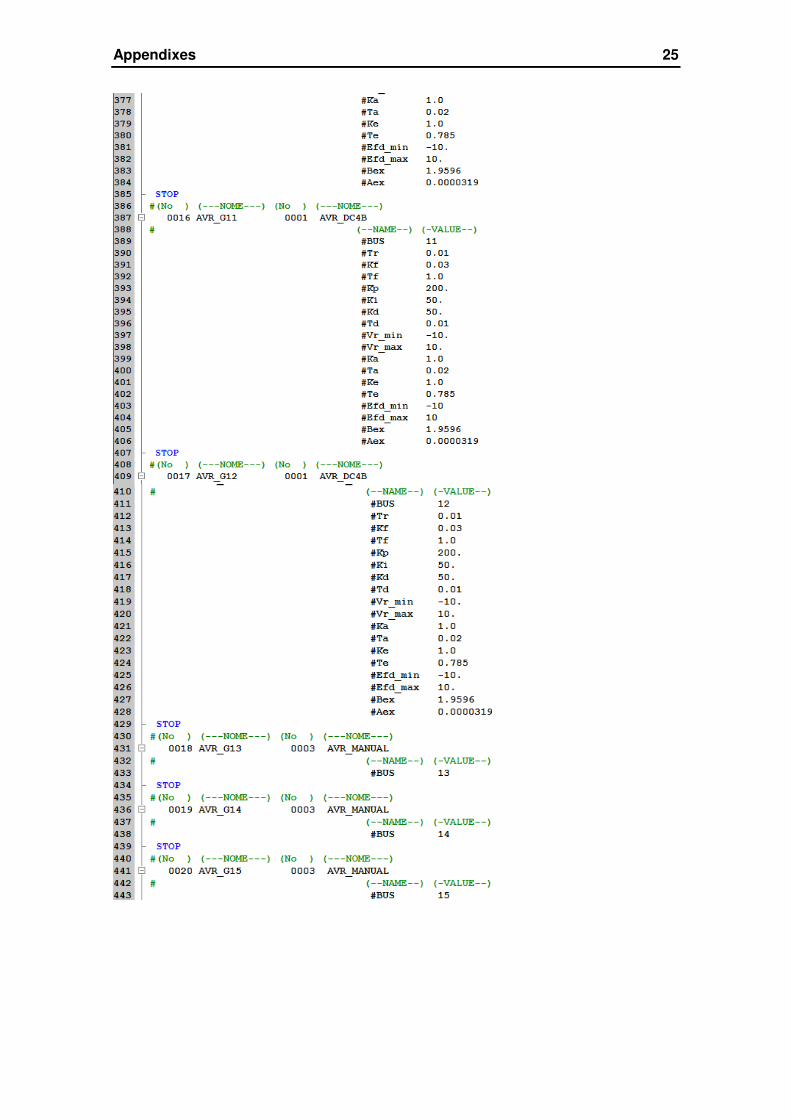
Note that, in Figure B-1 the generators parameters are inserted. In Figure B-2, the block
diagrams of the AVR and PSS are built, while in Figure B-3 controllers with their respective
parameters are related to their corresponding generators.
Figure B-1: Insertion of system data and definition of generator models.
20 Appendixes
Appendixes 21
Figure B-2: Building of AVR and PSS model.

22 Appendixes

Appendixes 23
24 Appendixes
Appendixes 25
26 Appendixes

Appendixes 27

28 Appendixes
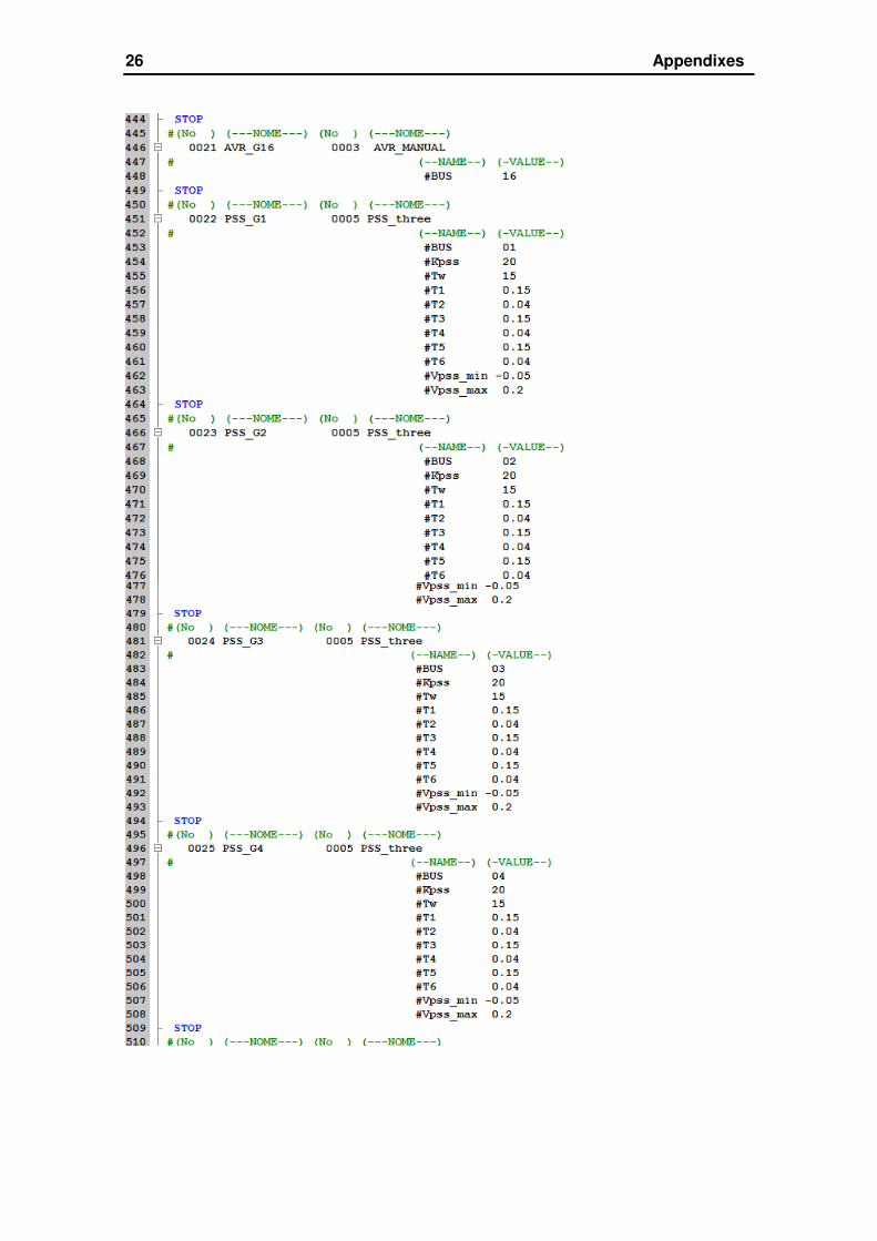
Figure B-3: Association of AVRs to their respective generators and insertion of the corresponding
parameters.
Appendix C
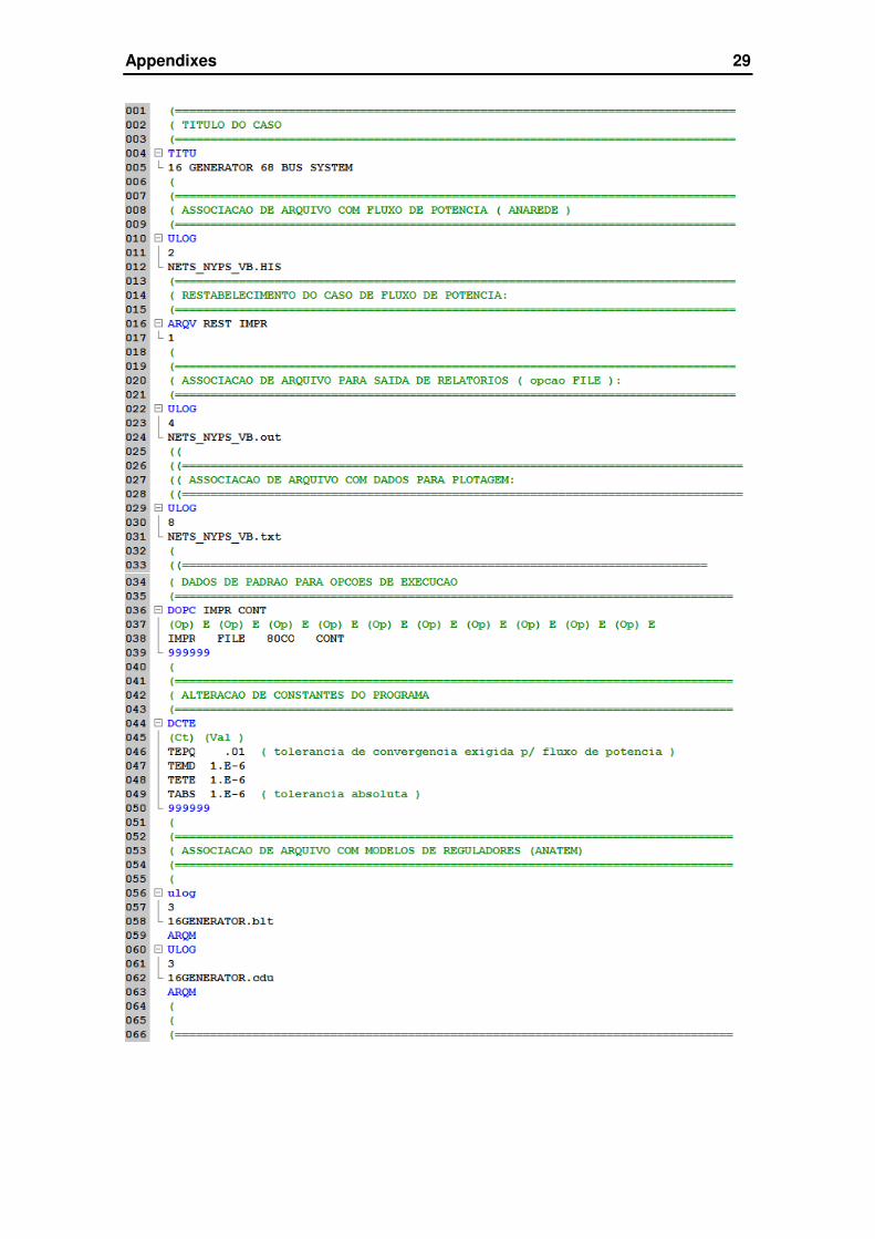
The main input file 68bus_ANATEM.STB used in the ANATEM software for
nonlinear simulation of the NETS-NYPS 68 Bus system is given in Figures C-1.
In this file, the associations with the files of steady-state operation (*.sav) from
ANAREDE, pre-defined machine models (*.blt) and user-defined controllers (*.cdu) are
depicted. This main file also contains the data for the applied perturbation and the
association with the output file (*.plt) that contains the output variables of interest.
Appendixes 29
30 Appendixes

Appendixes 31
Figure C-1: Main file (*.stb).
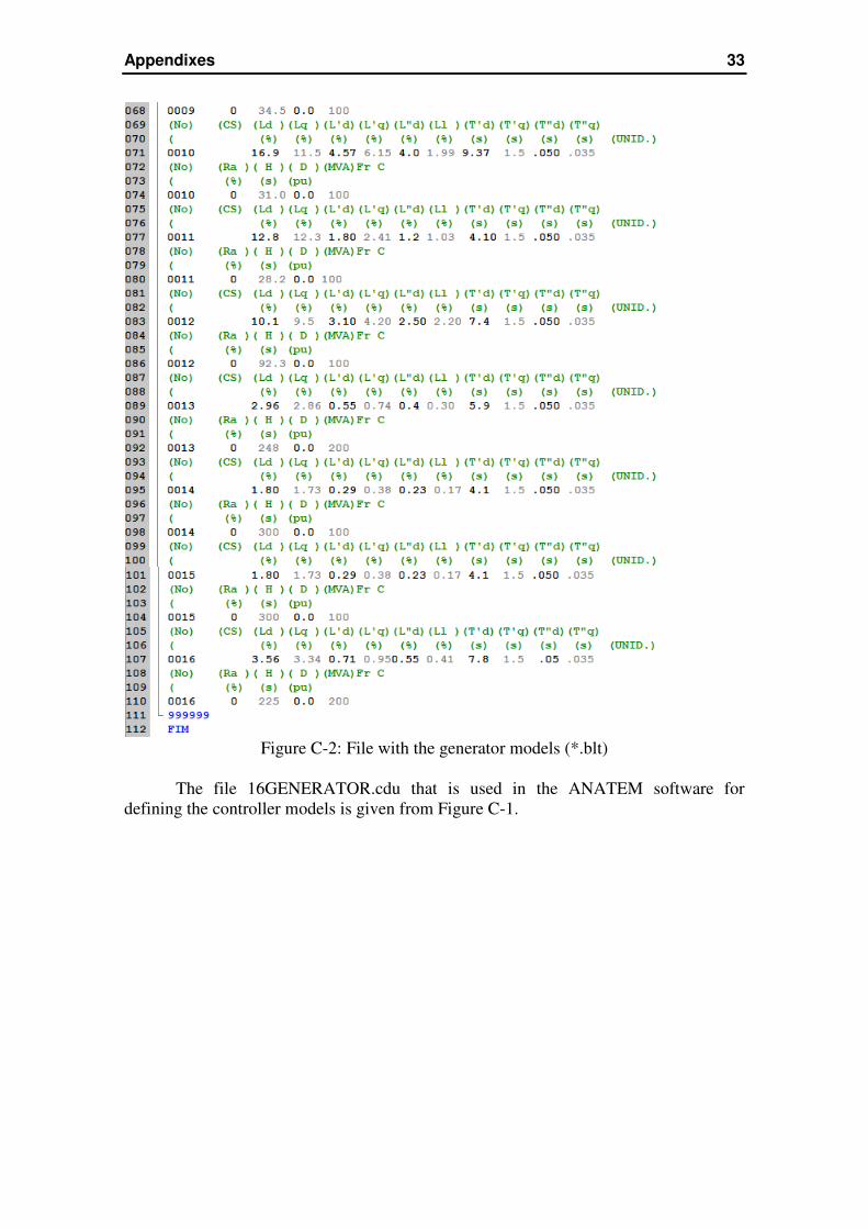
The input file 16GENERATOR.blt that is used in the ANATEM software for
nonlinear simulation of the NETS-NYPS 68 Bus system in given in Figure C-2.
32 Appendixes
Appendixes 33
Figure C-2: File with the generator models (*.blt)
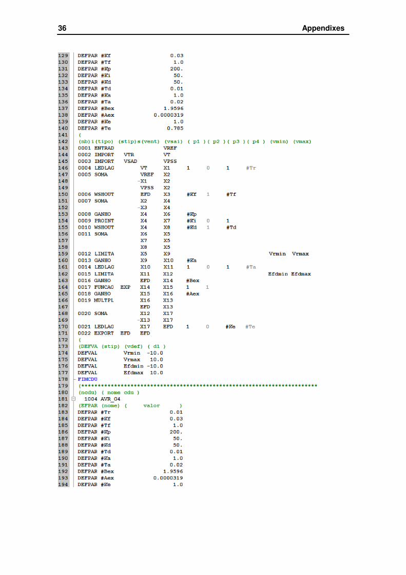
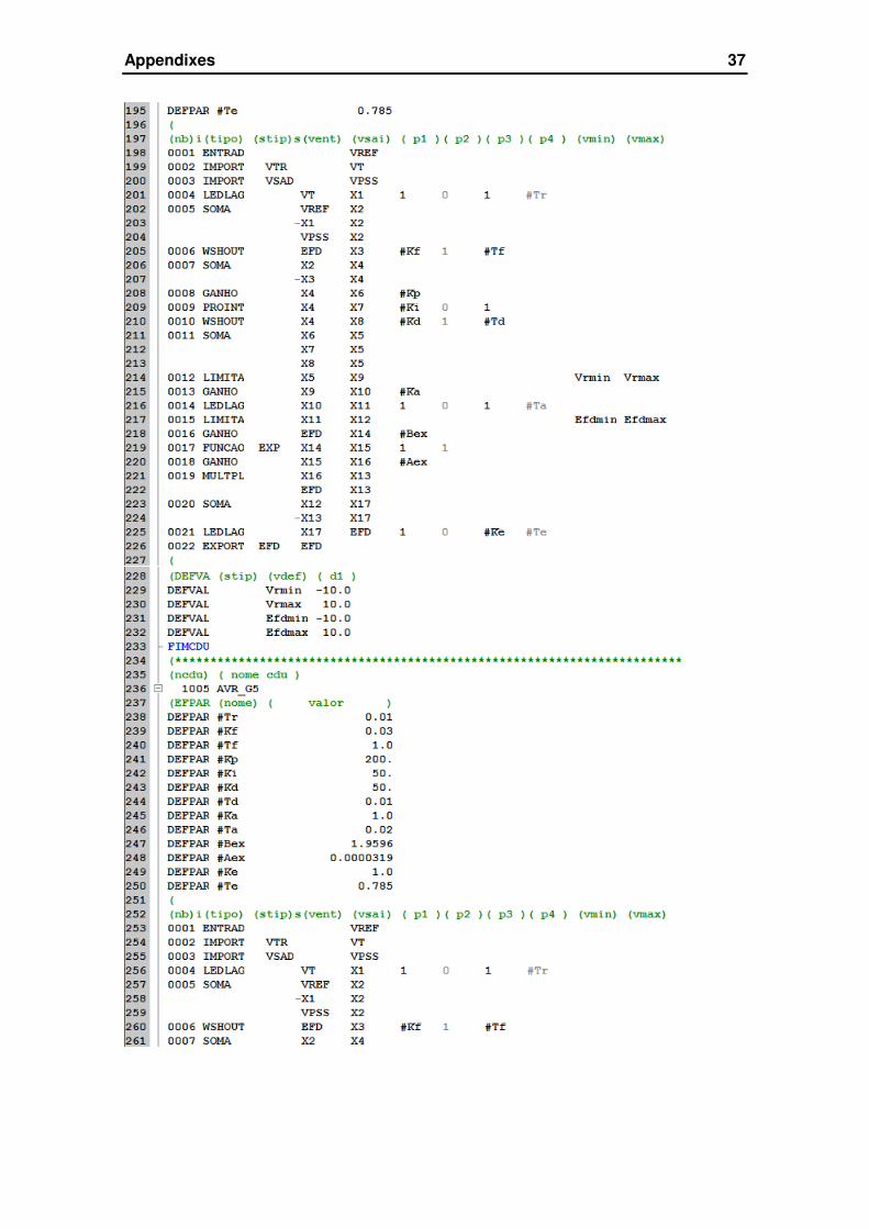
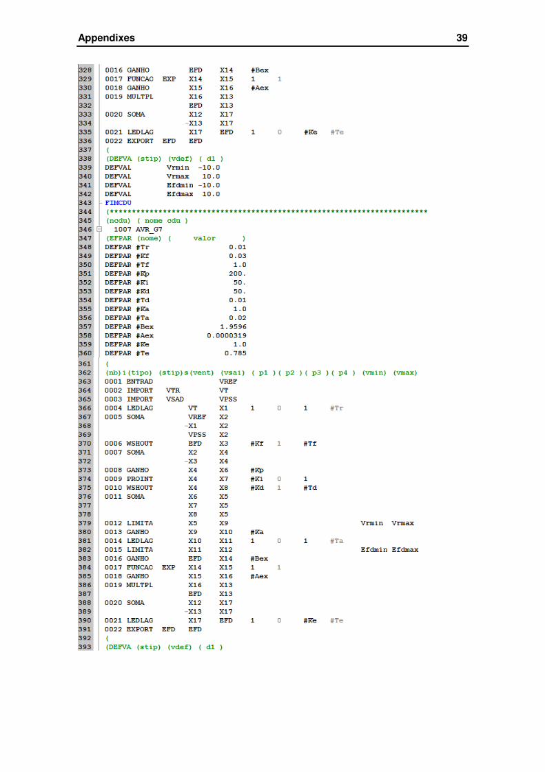
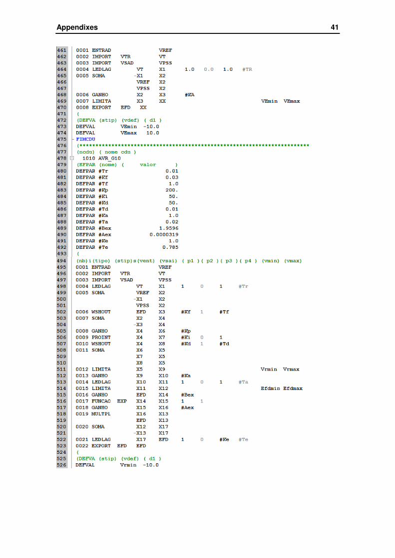
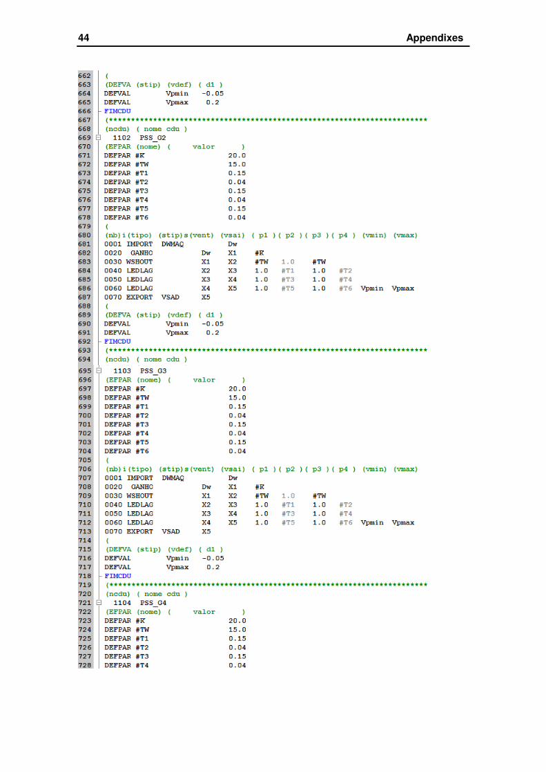
The file 16GENERATOR.cdu that is used in the ANATEM software for
defining the controller models is given from Figure C-1.

34 Appendixes

Appendixes 35
36 Appendixes
Appendixes 37

38 Appendixes
Appendixes 39

40 Appendixes
Appendixes 41

42 Appendixes

Appendixes 43
44 Appendixes

Appendixes 45

46 Appendixes

Appendixes 47

48 Appendixes
Figure C-1: Models of voltage regulators for the generators (*.cdu file).
References
[1] B. Pal and B. Chaudhuri, Robust Control in Power Systems. New York, U.S.A.: Springer,
2005, chapter 4.
[2] CEPEL, Centro de Pesquisas em Energia Elétrica. Rio de Janeiro, RJ, 2002. PACDYN –
On-Line Manual (in English). Available in http://www.pacdyn.cepel.br. Accessed in July 11,
2013.
[3] B. C. Pal, and A. K. Singh. IEEE PES Task Force on Benchmark Systems for Stability
Controls – Report on the 68-Bus, 16-Machine, 5-Area System. Version 3.3, Dec., 2013.
[4] P. Kundur, Power System Stability and Control. New York: McGraw-Hill, 1994.