IE 312 ROLLING LAB

Technical Report Submitted to: Dept. of Industrial and Manufacturing Engineering

Prof. Edward C De Meter

310 Leonhard Building

The Pennsylvania State University

University Park, PA 16802

Submitted by:

Team: 4; Section: 2

Michael McCallops

Thomas Hartmann

Kevin Arbuckle

Mark Savidge

Ryan Carlson

Date: April 15, 2016

1

Table of Contents Page #

Investigation Results:

1) Data Analysis

a. Ratio Analysis of the Wide Sample Rolling Processes 2

b. Surface Finish and Flatness Errors Derived from Rolling the Wide Samples 4

c. Impact of Width-to-Thickness Ratio on Deformation Behavior 6

d. Mechanical Analysis of the Brass Rolling Process 7

i. Hardness to UTS Conversion 7

ii. Derivation of Rolling Flow Stress Equation 8

iii. Mechanical Analysis 9

e. Derivation of the Coefficient of Friction 9

2) References 9

3) Appendix 10

2

Ratio Analysis of the Wide Sample Rolling Processes

Aluminum Wide Specimen:

Table 1. Aluminum Calculations

Brass Wide Specimen:

Table 2. Brass Calculations

Figure 1. Width to Thickness Ratio Curve

For the data on the width to thickness ratio the curve is a on a smooth increase for both aluminum and the brass. What this shows is that during each pass the width of the piece would increase slightly and the thickness would therefore decrease giving it a smooth arc.

Pass Width Average Thick Avg WTR RR SR0 1.058166667 0.126 8.398148148 0 01 1.058333333 0.123833333 8.546433378 0.017496635 0.0001575052 1.058666667 0.111833333 9.466467958 0.107302534 0.0003149613 1.061 0.096 11.05208333 0.164930556 0.002204034 1.062333333 0.082833333 12.8249497 0.158953722 0.0012566765 1.063833333 0.065 16.36666667 0.274358974 0.001411986

Pass Width Average Thick Avg WTR RR SR0 1.002833333 0.125 8.022666667 0 01 1.002833333 0.115333333 8.695086705 0.083815029 02 1.005 0.103 9.757281553 0.1197411 0.0021605453 1.005166667 0.093333333 10.76964286 0.103571429 0.0001658374 1.006333333 0.080833333 12.44948454 0.154639175 0.001160675 1.009333333 0.069166667 14.59277108 0.168674699 0.00298112

3

Figure 2. Spread Ratio Curve

For both materials the spread ratio did not generate a graph with any noticeable trends. The change in width from pass to pass varied amounts giving data that generated the graph above. This could be due to minor changes in the machine or imperfections in the metal.

Figure 3. Reduction Ratio Curve

For brass, the change in thickness compared to the previous thickness became greater throughout the passes compared to aluminum. When brass is rolled, the grain structure is more greatly changed than that of aluminum. The grains become larger allowing brass to be more easily formed. Both materials appear to show a roughly linear trend. According to how reduction ratio is calculated, we would expect there to be a positive correlation.

4

Surface Finish and Flatness Errors Derived from Rolling the Wide Samples

You are to create a table that lists the average arithmetic surface roughness for each wide sample before it was rolled and after it completed the fifth rolling pass.

Brass Specimen:

Table 3. Brass Surface Roughness Calculations

RA #1 (uin) RA #2 (uin) RA #2 (uin) Averages (uin)

Pass #0 120 110 115 115

Pass #5 15 20 19 18

Aluminum Specimen:

Table 4. Brass Surface Roughness Calculations

RA #1 (uin) RA #2 (uin) RA #2 (uin) Averages (uin)

Pass #0 129 115 123 122.3

Pass #5 18 33 26 25.7

Using this data as a basis, you are to explain whether the cold rolling process either improved the surface finish or degraded it.

Because the average surface roughness decreased from 115 uin to 18 uin after 5 passes through cold rollers, for total a decrease of 97 uin, the cold rolling process improved the surface finish by making the surface more uniform. It is noticeable that the cold rolling process significantly decreases the arithmetic surface roughness as more rolls are administered.

You are to also explain what physical mechanism resulted in the changed surface finish.

This changed surface finish is due to deformation. The rollers put large amounts of normal force on the small asperities on the surface of the metal; this causes these asperities to deform and flatten, making the piece more uniform.

You are to then comment on the severity of the flatness errors of the two samples that were rolled. Use the photos illustrating the samples on edge before and after the first rolling pass to 12 reinforce your discussion. If the flatness errors appear severe, offer a technical explanation for their cause.

Figure 4. Brass and Aluminum Specimens

5

The flatness error of the aluminum was significantly more than the error of the brass. The aluminum also elongated more than the brass workpiece as well.

The flatness errors in this piece were created due to internal stresses in the workpiece. As the piece is rolled through the cold rollers, the internal forces attempt to balance themselves under the increased normal forces applied to them. This results in the bending/warping of the workpiece after it is rolled.

Likewise discuss how these types of flatness errors are mitigated in industrial rolling processes.

Leveling rollers are typically used in industrial rolling processes, where several rollers are placed in succession with a smaller gaps in between each pair of rollers. This is usually used in industrial rolling processes to reduce the flatness error.

Figure 5. Rolling Procedures

6

Impact of Width-to-Thickness Ratio on Deformation Behavior

Table 5 was calculated by taking the averages for the width and thickness measurements for all four materials. Then using these averages and the below equations, these ratios were calculated:

wtr = Wo/To width-to-thickness

d = To – Tf draft

rr = d/To reduction ratio

s = Wf – Wo spread

sr = s/Wo spread ratio

Analysis:

The higher the width-to-thickness ratio, the lower the spread ratio. Vice versa is also true. Therefore, the narrow pieces had a higher spread ratio because their width-to-thickness ratio was lower than that of the wide pieces. This supports the notion that as width-to-thickness increases, the strain becomes more planar. This is because when the material has a lower width-to-thickness ratio the material will spread easier because there is less resistance. This translates to a higher spread ratio. When the width-to-thickness ratio is higher, more planar strain is required in order to spread the material, which is why the spread ratio is lower. The reduction ratio was not majorly effected by the width-to-thickness ratio as the values were relatively close for all the samples, and there doesn’t seem to be a correlation between the two. This is because the change in thickness for all the materials is close to the same. The only major difference between the reduction ratio between the two materials is caused by the difference in the elastic modulus and Poisson’s ratio between the two materials.

Table 5. Aluminum and Brass Calculations

7

Mechanical Analysis of the Brass Rolling Process

Hardness to UTS Conversion

In this lab, we were given data that contained HR30T to HRB conversions and HRB to UTS conversions. Using a regression equation with our conversion data, we were able to apply regression equations to the data in order to create lines of best fit. The scatter plots and trend line equations can be seen below. The plot below displays the hardness conversion equations for HR 30T to HRB, Figure 6. Figure 7 shows the conversion for HRB to UTS.

Figure 6. HRB vs HR 30T Graph

Figure 7. UTS (kpsi) vs HRB Graph

8

We then created a scatter plot that has the brass hardness values as the independent variable against the converted ultimate tensile strength values. This conversion can be seen below in Figure 8 along with the trend line equation.

Derivation of Rolling Flow Stress Equation

We created a flow stress curve based on the true strain and ultimate tensile strength. The graph in Figure 9 along with the flow stress equation can be seen below.

The trend line shows that the coefficients for the flow stress equation are K = 73.342 and η = 0.1162.

Figure 8. HR 30T to UTS (For Brass)

Figure 9. Flow Stress Equation Trendline

9

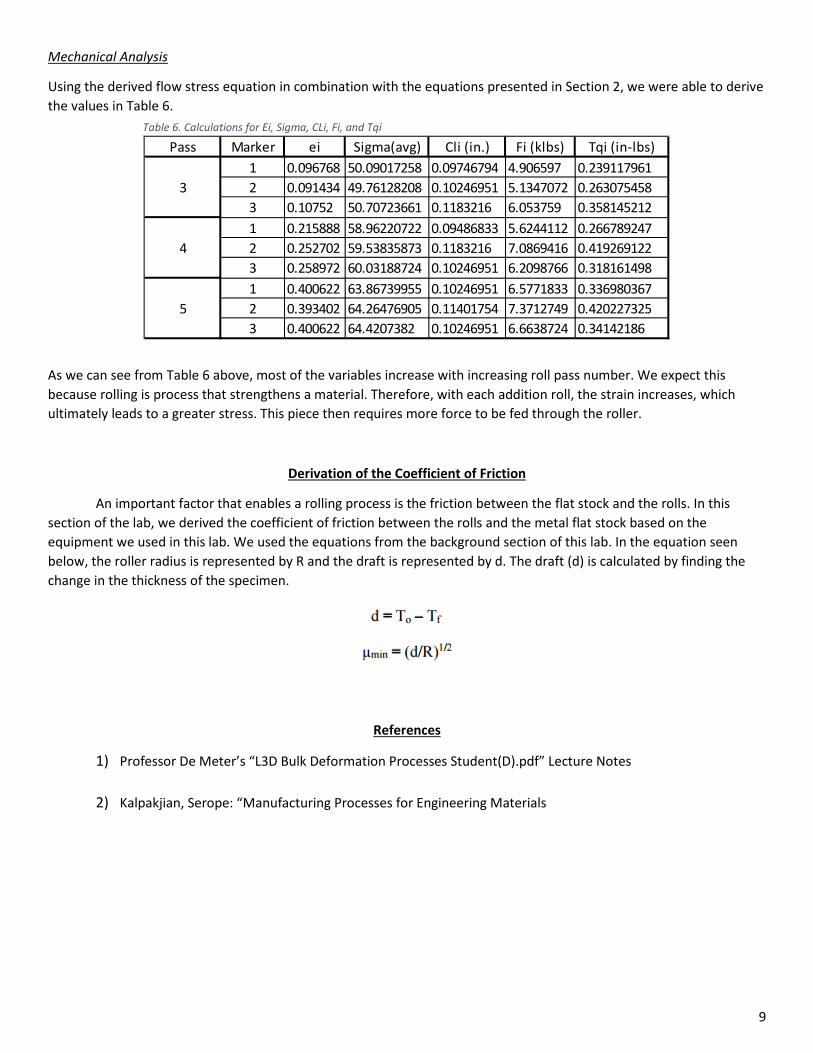
Mechanical Analysis

Using the derived flow stress equation in combination with the equations presented in Section 2, we were able to derive the values in Table 6.

As we can see from Table 6 above, most of the variables increase with increasing roll pass number. We expect this because rolling is process that strengthens a material. Therefore, with each addition roll, the strain increases, which ultimately leads to a greater stress. This piece then requires more force to be fed through the roller.

Derivation of the Coefficient of Friction

An important factor that enables a rolling process is the friction between the flat stock and the rolls. In this section of the lab, we derived the coefficient of friction between the rolls and the metal flat stock based on the equipment we used in this lab. We used the equations from the background section of this lab. In the equation seen below, the roller radius is represented by R and the draft is represented by d. The draft (d) is calculated by finding the change in the thickness of the specimen.

References

1) Professor De Meter’s “L3D Bulk Deformation Processes Student(D).pdf” Lecture Notes

2) Kalpakjian, Serope: “Manufacturing Processes for Engineering Materials

Pass Marker ei Sigma(avg) Cli (in.) Fi (klbs) Tqi (in-lbs)1 0.096768 50.09017258 0.09746794 4.906597 0.2391179612 0.091434 49.76128208 0.10246951 5.1347072 0.2630754583 0.10752 50.70723661 0.1183216 6.053759 0.3581452121 0.215888 58.96220722 0.09486833 5.6244112 0.2667892472 0.252702 59.53835873 0.1183216 7.0869416 0.4192691223 0.258972 60.03188724 0.10246951 6.2098766 0.3181614981 0.400622 63.86739955 0.10246951 6.5771833 0.3369803672 0.393402 64.26476905 0.11401754 7.3712749 0.4202273253 0.400622 64.4207382 0.10246951 6.6638724 0.34142186

3

4

5

Table 6. Calculations for Ei, Sigma, CLi, Fi, and Tqi

10

Appendix

Tables A1-A8:

11