IDL: A Possible Alternative to Matlab?Ecaterina Coman

Department of Mathematics and Statistics, University of Maryland, Baltimore County

Senior Thesis, Spring 2012

Thesis mentor Dr. Matthias K.Gobbert

Abstract

Created by Exelis Visual Information Solutions, IDL (Interactive Data Language) isa commercial package used for data analysis. We compared the usability and efficiencyof IDL to that of Matlab to determine if IDL is a viable substitute. Two studies wereperformed for this analysis. The first, a basic test inspired by the CIRC Tutorial forBasic Matlab, consisted of solving a system of linear equations using basic operations,computing eigenvalues and eigenvectors, and creating two-dimensional plots. It showedidentical results between the two packages, though it is important to note that thesyntax and display of output between IDL and Matlab differs greatly. The second testfocused on direct and iterative solutions of a large sparse system of linear equations.This system arises from the finite difference discretization of the Poisson equationwith homogeneous Dirichlet boundary conditions and is prototypical for linear systemsin many related contexts. In Matlab, Gaussian elimination was used as the directmethod of solving the Poisson test problem. Unfortunately, such a method was notavailable with our license of IDL to solve sparse systems as it required a more expensiveIDL Analyst License. Originally, we aimed to solve the problem iteratively using theconjugate gradient method, but, though a function was available in Matlab for solvinga sparse system this way, none existed in IDL. Instead, we turned to the biconjugategradient method. The numerical results of this method in IDL are identical to those inMatlab, but IDL runs the code slightly faster for finer meshes. Those looking to make aswitch from Matlab to IDL might have a difficult time encountering a different syntax,output display, and the need for a more expensive license to run a larger breadth offunctions or procedures, but if efficiency is of concern, IDL can potentially be fasterthan Matlab.

1 Introduction

1.1 Overview

There are several numerical computational packages that serve as educational tools and arealso available for commercial use. Matlab is the most widely used such package. The focus ofthis study is to introduce an additional numerical computational package, IDL, and provideinformation on whether or not this package is compatible to Matlab and can be used asan alternative. Section 1.3 provides a more detailed description of these two packages. Toevaluate IDL, a comparative approach is used based on a Matlab user’s perspective. Toachieve this task, we perform some basic and some complex studies on Matlab and IDL.

1

The basic studies include basic operations solving systems of linear equations, computingthe eigenvalues and eigenvectors of a matrix, and two-dimensional plotting. The complexstudies include direct and iterative solutions of a large sparse system of linear equationsresulting from finite difference discretization of an elliptic test problem.

In Section 2, we perform the basic operations test using Matlab and IDL. This includestesting the backslash operator, computing eigenvalues and eigenvectors, and plotting in twodimensions. The backslash operator works easily in Matlab to produce a solution to thelinear system given. Instead of the backslash operator, the LUDC and LUSOL commandsare used in IDL to compute the LU decomposition and use its result to solve the system.The command eig computes eigenvalues and eigenvectors in Matlab, whereas IDL requiresa three-step process. IDL uses ELMHES to reduce the matrix to upper Hessenberg format,and then HQR to compute the eigenvalues. Given the eigenvalues, EIGENVEC then gives theeigenvectors. Plotting is another important feature we analyze by an m-file containing thetwo-dimensional plot function along with some common annotation commands. Like Matlab,IDL uses a basic plot command to create the 2D plot, but one has to use quite different,but equivalent commands for annotation.

Section 3 introduces a common test problem, given by the Poisson equation with homo-geneous Dirichlet boundary conditions, and discusses the finite discretization for the problemin two dimensional space. In the process of finding the solution, we use a direct method,Gaussian elimination, and an iterative method, the biconjugate gradient method. To be ableto analyze the performance of these methods, we solve the problem on progressively finermeshes. The Gaussian elimination method built into the backslash operator successfullysolves the problem up to a mesh resolution of 4,096 × 4,096 in Matlab, but in IDL theredoes not exist a Gaussian elimination method for sparse matrices without an expensive IDLAnalyst license. For this reason, the IDL Gaussian elimination test was not conducted. Wehad originally planned a comparison using the conjugate gradient iterative method in bothMatlab and IDL, but such a method did not exist in IDL for solving sparse systems. For thisreason, the biconjugate gradient method was used in both packages for comparison. Thebiconjugate gradient method is available in the bicg function in Matlab and in IDL throughthe command LINBCG. The sparse matrix implementation of the iterative method allows usto solve a mesh resolution up to 8,192× 8,192 in Matlab and IDL. The existence of the mesh

in Matlab allows us to include the three-dimensional plots of the numerical solution and thenumerical error. In IDL, the SURFACE plots match those of Matlab. IDL showed to be quitedifferent from Matlab when considering syntax. Many of the commands were either entirelyunavailable for our license (kron) or had to be applied differently (no backslash operatorresulted in the use of LUDC and LUSOL, and the lack of an eig function led to the use ofELMHES, HQR, and EIGENVEC). The tests focused on usability lead us to conclude that thepackage is not too compatible with Matlab, since it does not use the same syntax and somefunctions are not available. Is it important to note that, even though syntax is different,IDL is able to solve the same problems as Matlab.

Fundamentally, Matlab and IDL turn out to be able to solve complex problems of thesame size, as measured by the mesh resolution of the problem. Matlab and IDL also tookabout the same time to solve the problem, though IDL was slightly faster. The data that

2

these conclusions are based on are summarized in Tables 3.1 and 3.2.The next section contains some additional remarks on features of the software packages

that might be useful, but go beyond the tests performed in Sections 2 and 3. Sections 1.3and 1.4 describe the two numerical computational packages in more detail and specify thecomputing environment used for the computational experiments, respectively.

1.2 Additional Remarks: Ordinary Differential Equations

One important feature to test would be the ODE solvers in the packages under considera-tion. For non-stiff ODEs, Matlab has three solvers: ode113, ode23, and ode45 implement anAdams-Bashforth-Moulton PECE solver and explicit Runge-Kutta formulas of orders 2 and4, respectively. For stiff ODEs, Matlab has four ODE solvers: ode15s, ode23s, ode23t, andode23tb implement the numerical differentiation formulas, a Rosenbrock formula, a trape-zoidal rule using a “free” interpolant, and an implicit Runge-Kutta formula, respectively.

With the availability of an IDL Analyst License, IDL also has ODE solvers. For a possiblystiff ODE, IMSL_ODE implements the Adams-Gear method. If known that the problem is notstiff, a keyword to this command can use the Runge-Kutta-Verner methods or orders 4 and 6instead. There also exist outside functions, such as DDEABM written by Craig Markwardt usingan adaptive Adams-Bashford-Moulton method to solve primarily non-stiff and mildly stiffODE problems or RunKut_step written by Frank Varosi using a fourth order Runge-Kuttamethod.

It becomes clear that all software packages considered have at least one solver. Matlaband IDL have state-of-the-art variable-order, variable-timestep methods for both non-stiffand stiff ODEs available, with Matlab’s implementation being the richest and its stiff solversbeing possibly more efficient.

1.3 Description of the Packages

1.3.1 Matlab

“MATLAB is a high-level language and interactive environment that enables one to performcomputationally intensive tasks faster than with traditional programming languages suchas C, C++, and Fortran.” The web page of the MathWorks, Inc. at www.mathworks.

com states that Matlab was originally created by Cleve Moler, a Numerical Analyst in theComputer Science Department at the University of New Mexico. The first intended usage ofMatlab, also known as Matrix Laboratory, was to make LINPACK and EISPACK availableto students without facing the difficulty of learning to use Fortran. Steve Bangert and JackLittle, along with Cleve Moler, recognized the potential and future of this software, which ledto establishment of MathWorks in 1983. As the web page states, the main features of Matlabinclude high-level language; 2-D/3-D graphics; mathematical functions for various fields;interactive tools for iterative exploration, design, and problem solving; as well as functionsfor integrating MATLAB-based algorithms with external applications and languages. Inaddition, Matlab performs the numerical linear algebra computations using for instanceBasic Linear Algebra Subroutines (BLAS) and Linear Algebra Package (LAPACK).

3

1.3.2 IDL

IDL (Interactive Data Language) was created by Exelis Visual Information Solutions, for-merly ITT Visual Information Solutions. The webpage for Exelis at www.exelisvis.com

states that IDL can be used to create meaningful visualizations out of complex numericaldata, processing large amounts of data interactively. IDL is an array-oriented, dynamiclanguage with support for common image formats, hierarchical scientific data formats, and.mp4 and .avi video formats. IDL also has functionality for 2D/3D gridding and interpola-tion, routines for curve and surface fitting, and the capability of performing multi-threadedcomputations.

IDL can be run on Windows, Mac OS X, Linux, and Solaris platforms. It can bedownloaded from the Exelis webpage at http://www.exelisvis.com/language/en-US/

Downloads/ProductDownloads.aspx after registering.

1.4 Description of the Computing Environment

The computations for this study are performed using Matlab R2011a and IDL 8.1 under theLinux operating system Redhat Enterprise Linux 5. The Cluster tara in the UMBC HighPerformance Computing Facility (www.umbc.edu/hpcf) is used to carry out the computa-tions and has a total of 86 nodes, with 82 used for computation. Each node features twoquad-core Intel Nehalem X5550 processors (2.66 GHz, 8,192 kB cache per core) with 24 GBof memory.

4

2 Basic Operations Test

This section examines a collection of examples inspired by some basic mathematics courses.This set of examples was originally developed for Matlab by the Center for InterdisciplinaryResearch and Consulting (CIRC). More information about CIRC can be found at www.umbc.edu/circ. This section focuses on the testing of basic operations using Matlab and IDL.We will first begin by solving a linear system; then finding eigenvalues and eigenvectors of asquare matrix; and finally, 2-D functional plotting.

2.1 Basic operations in Matlab

This section discusses the results obtained using Matlab operations. To run Matlab onthe cluster tara, enter matlab at the Linux command line. This starts up Matlab with itscomplete Java desktop interface. Useful options to Matlab on tara include -nodesktop,which starts only the command window within the shell, and -nodisplay, which disablesall graphics output. For complete information on options, use matlab -h.

2.1.1 Solving Systems of Equations

The first example that we will consider in this section is solving a linear system. Considerthe system of equations

−x2 + x3 = 3,

x1 − x2 − x3 = 0,

−x1 − x3 = −3,

whose solution is (1,−1, 2)T . In order to use Matlab to solve this system, let us express thislinear system as a single matrix equation

Ax = b (2.1)

where A is a square matrix consisting of the coefficients of the unknowns, x is the vector ofunknowns, and b is the right-hand side vector. For this particular system, we have

A =

0 −1 11 −1 −1−1 0 −1

, b =

30−3

.

To find a solution for this system in Matlab, left divide (2.1) by A to obtain x = A\b. Hence,Matlab use the backslash operator to solve this system. First, the matrix A and vector b areentered using the following:

A = [0 -1 1; 1 -1 -1; -1 0 -1]

b = [3;0;-3].

5

Now use x = A\b to solve this system. The resulting vector which is assigned to x is:

x =

1

-1

2

Notice the solution is exactly what was expected based on our hand computations.

2.1.2 Calculating Eigenvalues and Eigenvectors

Here, we will consider another important function: computing eigenvalues and eigenvectors.Finding the eigenvalues and eigenvectors is a concept first introduced in a basic LinearAlgebra course and we will begin by recalling the definition. Let A ∈ Cn×n and v ∈ Cn. Avector v is called the eigenvector of A if v 6= 0 and Av is a multiple of v; that is, there existsa λ ∈ C such that

Av = λv

where λ is the eigenvalue of A associated with the eigenvector v. We will use Matlab tocompute the eigenvalues and a set of eigenvectors of a square matrix. Let us consider amatrix

A =

[1 −11 1

]which is a small matrix that we can easily compute the eigenvalues to check our results.Calculating the eigenvalues using det(A − λI) = 0 gives 1 + i and 1 − i. Now we will useMatlab’s built in function eig to compute the eigenvalues. First enter the matrix A andthen calculate the eigenvalues using the following commands:

A = [1 -1; 1 1];

v = eig(A)

The following are the eigenvalues that are obtained for matrix A using the commands statedabove:

v =

1.0000 + 1.0000i

1.0000 - 1.0000i

To check if the components of this vector are identical to the analytic eigenvalues, we cancompute

v - [1+i;1-i]

and it results in

ans =

0

0

6

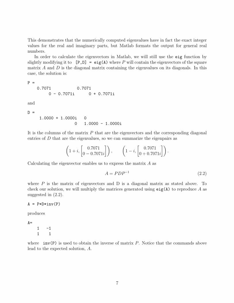
This demonstrates that the numerically computed eigenvalues have in fact the exact integervalues for the real and imaginary parts, but Matlab formats the output for general realnumbers.

In order to calculate the eigenvectors in Matlab, we will still use the eig function byslightly modifying it to [P,D] = eig(A) where P will contain the eigenvectors of the squarematrix A and D is the diagonal matrix containing the eigenvalues on its diagonals. In thiscase, the solution is:

P =

0.7071 0.7071

0 - 0.7071i 0 + 0.7071i

and

D =

1.0000 + 1.0000i 0

0 1.0000 - 1.0000i

It is the columns of the matrix P that are the eigenvectors and the corresponding diagonalentries of D that are the eigenvalues, so we can summarize the eigenpairs as(

1 + i,

[0.7071

0− 0.7071i

]),

(1− i,

[0.7071

0 + 0.7071i

]).

Calculating the eigenvector enables us to express the matrix A as

A = PDP−1 (2.2)

where P is the matrix of eigenvectors and D is a diagonal matrix as stated above. Tocheck our solution, we will multiply the matrices generated using eig(A) to reproduce A assuggested in (2.2).

A = P*D*inv(P)

produces

A=

1 -1

1 1

where inv(P) is used to obtain the inverse of matrix P . Notice that the commands abovelead to the expected solution, A.

7

(a) (b)

Figure 2.1: Plots of f(x) = x sin(x2) in Matlab using (a) 129 and (b) 1025 equally spaceddata points.

2.1.3 2-D Plotting

2-D plotting is a very important feature as it appears in all mathematical courses. Sincethis is a very commonly used feature , let us examine the 2-D plotting feature of Matlabby plotting f(x) = x sin(x2) over the interval [−2π, 2π]. The data set for this functionis given in the data file matlabdata.dat and is posted along with the tech. report [3] atwww.umbc.edu/hpcf under Publications. Noticing that the data is given in two columns,we will first store the data in a matrix A. Second, we will create two vectors, x and y, byextracting the data from the columns of A. Lastly, we will plot the data.

A = load (’matlabdata.dat’);

x = A(:,1);

y = A(:,2);

plot(x,y)

The commands stated above result in the Figure 2.1 (a). Looking at this figure, it can benoted that our axes are not labeled; there are no grid lines; and the peaks of the curves arerather coarse. The title, grid lines, and axes labels can be easily created. Let us begin bylabeling the axes using xlabel(’x’) to label the x-axis and ylabel(’f(x)’) to label they-axis. axis on and grid on can be used to create the axis and the grid lines. The axesare on by default and we can turn them off if necessary using axis off. Let us also createa title for this graph using title (’Graph of f(x)=x sin(x^2)’). We have taken care ofthe missing annotations and lets try to improve the coarseness of the peaks in Figure 2.1 (a).We use length(x) to determine that 129 data points were used to create the graph of f(x).To improve this outcome, we can begin by improving our resolution using

x = [-2*pi : 4*pi/1024 : 2*pi];

to create a vector 1025 equally spaced data points over the interval [−2π, 2π]. In order tocreate vector y consisting of corresponding y values, use

8

y = x .* sin(x.^2);

where .* performs element-wise multiplication and .^ corresponds to element-wise arraypower. Then, simply use plot(x,y) to plot the data. Use the annotation techniques men-tioned earlier to annotate the plot. In addition to the other annotations, usexlim([-2*pi 2*pi]) to set limit is for the x-axis. We can change the line width to 2 byplot(x,y,’LineWidth’,2). Finally, Figure 2.1 (b) is the resulting figure with higher resolu-tion as well as the annotations. Observe that by controlling the resolution in Figure 2.1 (b),we have created a smoother plot of the function f(x). The Matlab code used to create theannotated figure is as follows:

x = [-2*pi : 4*pi/1024 : 2*pi];

y = x.*sin(x.^2);

H = plot(x,y);

set(H,’LineWidth’,2)

axis on

grid on

title (’Graph of f(x)=x sin(x^2)

xlabel (’x’)

ylabel (’f(x)’)

xlim ([-2*pi 2*pi])

2.1.4 Programming

Here we will look at a basic example of Matlab programming using a script file. Let’s tryto plot Figure 2.1 (b) using a script file called plotxsinx.m. The extension .m indicates toMatlab that this is an executable m-file. Instead of typing multiple commands in Matlab,we will collect these commands into a script. Now, call the script from the command-line toexecute it and create the plot with the annotations for f(x) = x sin(x2). The plot obtainedin this case is Figure 2.1 (b). This plot can be printed to a graphics file using the command

print -djpeg file_name_here.jpg

2.2 Basic operations in IDL

In this section, we will perform the basic operations using IDL. From the command line,enter idl to run the package in command line mode, or idlde to run the full developmentenvironment. To enter IDL online help, use idlhelp from the Linux command line or ? atthe IDL command line.

We will again begin by solving the linear system Ax = b as in Section 2.1.1. Create thematrices in IDL using the commands

A=[[0.0,-1.0,1.0],[1.0,-1.0,-1.0],[-1.0,0.0,-1.0]]

b=[3.0,0.0,-3.0]

9

Unlike Matlab, IDL does not have a dedicated backslash command to solve systems of linearequations. Instead, IDL uses the LUDC procedure along with the LUSOL function. The LUDC

procedure finds the LU decomposition of the matrix of equations and outputs a permutationmatrix. Following the LUDC procedure, the LUSOL function is called, with inputs includingthe matrix A, the vector of row permutations, and the column vector b. All matrices mustbe of type float or double to run the LUDC and LUSOL commands, and b must be a columnvector to run LUDC. The following commands will solve the system of equations:

LUDC,A,index

x=LUSOL(A,index,b)

Here, index is an input vector that LUDC creates which contains a record of the rowpermutations. These commands give a result

1.00000 -1.00000 2.00000

which is a row representation of the solution vector

x =

1.00000−1.00000

2.00000

and is consistent with the manual calculations and previous computational software results.

Next, let us consider the operation of computing eigenvalues and eigenvectors. We will usethe matrix A introduced in Section 2.1.2. We will first use IDL’s ELMHES function to reducethe matrix A to upper Hessenberg format, after which we will compute the eigenvalues ofthis new, upper Hessenberg matrix using the IDL function HQR. To compute eigenvectors andresiduals, we will use the EIGENVEC function which takes inputs of the matrix A and the newmatrix of eigenvalues, and outputs the residual. The commands to obtain the eigenvaluesand eigenvectors are the following:

A=[[1.0,-1.0],[1.0,1.0]]

hesA = ELMHES(A)

eval = HQR(hesA)

evec = EIGENVEC(A,eval, /DOUBLE, RESIDUAL=residual)

The eigenvalues calculated by HQR are

(1.00000, -1.00000)(1.00000,1.00000)

and the eigenvectors are

(0.70710678,1.7677670e-21)(1.7677670e-21,0.70710678)

(-1.7677670e-21,0.70710678)(0.70710678,-1.7677670e-21)

10

(a) (b)

Figure 2.2: Plots of f(x) = x sin(x2) in IDL using (a) 129 and (b) 1025 equally spaced datapoints.

IDL outputs complex numbers in parentheses, with the first number being the real part andthe second the imaginary part. So, if we consider double-precision floating-point numbers onthe scale of 10−21 as 0, then the above output specifies the following eigenpairs in standardmathematical notation for complex numbers and rounded to fewer digits:(

1− i,

[0.70710.7071i

]),

(1 + i,

[0.7071i0.7071

]).

IDL outputs each eigenvector as a row vector, which is very different in appearance fromthe output produced by the other packages whose output is based on the matrix P, whosecolumns are the eigenvectors. We notice that the eigenvalues were output in reverse orderthan by Matlab. Taking this into account and also noting that multiplying by −i shows[0.7071i, 0.7071]T = [0.7071,−0.7071i]T , we see that the eigenpairs are the same as thosecomputed by Matlab.

We are able to express the matrix A as PDP−1, where P is the matrix of eigenvectors andD is the diagonal matrix of eigenvalues, to reproduce the matrix A. Remembering that IDLoutputs eigenvectors as row vectors, we turn the output matrix of eigenvectors into the matrixP by taking the transpose with the command P=transpose(evec) then use INVERT(P) toobtain the inverse of P . To create D, we create a matrix with the eigenvalues on the diagonal.This can easily be created with the command D=[[eval[0],0],[0,eval[1]]], which takesthe complex values in the vector of eigenvalues found using HQR and puts them on thediagonal. In IDL, the ## operator is used for matrix multiplication, and computing PDP−1

with the command P##diag##invert(P) gives a result of

(1.00000000,-0.00000000)(-1.00000000,0.00000000)

(1.00000000,0.00000000)(1.00000000,0.00000000)

which is A to at least 8 significant digits.Next, we will examine the similarities between the plotting commands using f(x) =

x sin(x2). To obtain data from a file, the following commands will get the number of lines in

11

the file and create a two-column double-type array to hold the data, open the file and createa logical unit number which will be associated with that opened file, read the data into thedouble array, and close the file and free the logical unit number:

nlines=FILE_LINES(’matlabdata.dat’)

data=DBLARR(2,nlines)

openr, lun, ’matlabdata.dat’, /get_lun

readf, lun, data

free_lun, lun

Using x=data(0,*) and y=data(1,*) will create vectors x and y The plot procedure,PLOT, x, y will then create Figure 2.2 (a) using vectors x and y. These commands have anobvious agreement to the LOAD and PLOT commands in matlab as Figure 2.2 (a) is the sameas Figure 2.1 (a). To annotate this graph, use the TITLE command to add a graph title, theXTITLE and YTITLE commands to add a horizontal and vertical axis title, respectively. Tocreate a grid, we use XTICKLEN and YTICKLEN and edit the line style using XGRIDSTYLE andYGRIDSTYLE. Now, we want to have a smoother graph made of more equally spaced datapoints. We create a second vector x using x=(4*!pi)*FINDGEN(1025)/1024 - (2*!pi),where FINDGEN creates an array of 1025 values from 0 to 1024, to get a range of numbersfrom −2π to 2π at intervals of pi. Using this new x, make the vector y with the commandy=x*sin(x^2). This annotated data can be plotted using

PLOT, x, y, XSTYLE=1, THICK=2, TITLE=’Graph of f(x)=xsin(x!E2!N)’, $

XTITLE=’x’, YTITLE=’f(x)’,XTICKLEN=1.0, YTICKLEN=1.0,$

XGRIDSTYLE=1, YGRIDSTYLE=1

The command XSTYLE=1 makes sure IDL is displaying the exact interval, as it normally wantsto produce even tick marks which create a wider range than desired. Also, the commandTHICK changes the thickness of the grid lines and $ is the line continuation character. Thisannotated plot procedure generates Figure 2.2 (b). These commands can all be placed intoa procedure file, which can run them all at once from the IDL command line. To save thisplot to a jpg file, save the contents of the current Direct Graphics window into a variableand write that variable using

image=tvrd()

write_jpeg, ’filename.jpg’, image

12

3 Complex Operations Test

3.1 The Test Problem

Starting in this section, we study a classical test problem given by the numerical solution withfinite differences for the Poisson problem with homogeneous Dirichlet boundary conditions [1,4, 5, 9], given as

−4u = f in Ω,u = 0 on ∂Ω.

(3.1)

This problem was studied before in, among other sources, [1,3,4,6–9]. Here ∂Ω denotes theboundary of the domain Ω while the Laplace operator is defined as

4u =∂2u

∂x2+

∂2u

∂y2.

This partial differential equation can be used to model heat flow, fluid flow, elasticity, andother phenomena [9]. Since u = 0 at the boundary in (3.1), we are looking at a homogeneousDirichlet boundary condition. We consider the problem on the two-dimensional unit squareΩ = (0, 1)× (0, 1) ⊂ R2. Thus, (3.1) can be restated as

−∂2u∂x2 − ∂2u

∂y2 = f(x, y) for 0 < x < 1, 0 < y < 1,

u(0, y) = u(x, 0) = u(1, y) = u(x, 1) = 0 for 0 < x < 1, 0 < y < 1,(3.2)

where the function f is given by

f(x, y) = −2π2 cos(2πx) sin2(πy)− 2π2 sin2(πx) cos(2πy).

The problem is designed to admit a closed-form solution as the true solution

u(x, y) = sin2(πx) sin2(πy).

3.2 Finite Difference Discretization

Let us define a grid of mesh points Ωh = (xi, yj) with xi = ih, i = 0, . . . , N + 1, yj = jh, j =0, . . . , N + 1 where h = 1

N+1. By applying the second-order finite difference approximation

to the x-derivative at all the interior points of Ωh, we obtain

∂2u

∂x2(xi, yi) ≈

u(xi−1, yj)− 2u(xi, yj) + u(xi+1, yj)

h2. (3.3)

If we also apply this to the y-derivative, we obtain

∂2u

∂y2(xi, yi) ≈

u(xi, yj−1)− 2u(xi, yj) + u(xi, yj+1)

h2. (3.4)

13

Now, we can apply (3.3) and (3.4) to (3.2) and obtain

− u(xi−1, yj)− 2u(xi, yj) + u(xi+1, yj)

h2

− u(xi, yj−1)− 2u(xi, yj) + u(xi, yj+1)

h2≈ f(xi, yj).

(3.5)

Hence, we are working with the following equations for the approximation ui,j ≈ u(xi, yj):

−ui−1,j − ui,j−1 + 4ui,j − ui+1,j − ui,j+1 = h2fi,j i, j = 1, . . . , Nu0,j = ui,0 = uN+1,j = ui,N+1 = 0

(3.6)

The equations in (3.6) can be organized into a linear system Au = b of N2 equations forthe approximations ui,j. Since we are given the boundary values, we can conclude there areexactly N2 unknowns. In this linear system, we have

A =

S −I−I S −I

. . . . . . . . .

−I S −I−I S

∈ RN2×N2

,

where

S =

4 −1−1 4 −1

. . . . . . . . .

−1 4 −1−1 4

∈ RN×Nand I =

1

1. . .

11

∈ RN×N

and the right-hand side vector bk = h2fi,j where k = i+(j−1)N . The matrix A is symmetricand positive definite [4, 9]. This implies that the linear system has a unique solution andit guarantees that the iterative Krylov subspace methods converge, of which the conjugategradient method as well as the biconjugate gradient method are examples.

To create the matrix A in Matlab effectively, we use the observation that it is given by asum of two Kronecker products [4, Section 6.3.3]: Namely, A can be interpreted as the sum

A =

T

T. . .

TT

+

2I −I−I 2I −I

. . . . . . . . .

p −I 2I −I−I 2I

∈ RN2×N2

,

where

T =

2 −1−1 2 −1

. . . . . . . . .

−1 2 −1−1 2

∈ RN×N

14

and I is the N ×N identity matrix, and each of the matrices in the sum can be computedby Kronecker products involving T and I, so that A = I ⊗ T + T ⊗ I.

One of the things to consider to confirm the convergence of the finite difference method isthe finite difference error. The finite difference error is defined as the difference between thetrue solution u(x, y) and the numerical solution uh defined on the mesh points by uh(xi, yj) =ui,j. Since the solution u is sufficiently smooth, we expect the finite difference error todecrease as N gets larger and h = 1

N+1gets smaller. Specifically, the finite difference theory

predicts that the error will converge as ‖u− uh‖L∞(Ω)≤ C h2, as h → 0, where C is a

constant independent of h [2, 5]. For sufficiently small h, we can then expect that the ratioof errors on consecutively refined meshes behaves like

Ratio =‖u− u2h‖‖u− uh‖

≈ C (2h)2

C h2= 4 (3.7)

Thus, we will print this ratio in the following tables in order to confirm convergence of thefinite difference method.

3.3 Matlab Results

3.3.1 Gaussian Elimination

Let us begin solving the linear system arising from the Poisson problem by Gaussian elimina-tion in Matlab. We know that this is easiest approach for solving linear systems for the userof Matlab, although it may not necessarily be the best method for large systems. To creatematrix A, we make use of the Kronecker tensor product, as described in Section 3.2. Thiscan be easily implemented in Matlab using the kron function. The matrix A is stored insparse storage mode, which does not store the zeros in the matrix. The system is then solvedusing the backslash operator. Figure 3.1 shows the results of this for a mesh with N = 32.

(a) (b)

Figure 3.1: Mesh plots for N = 32 in Matlab (a) of the numerical solution and (b) of thenumerical error.

15

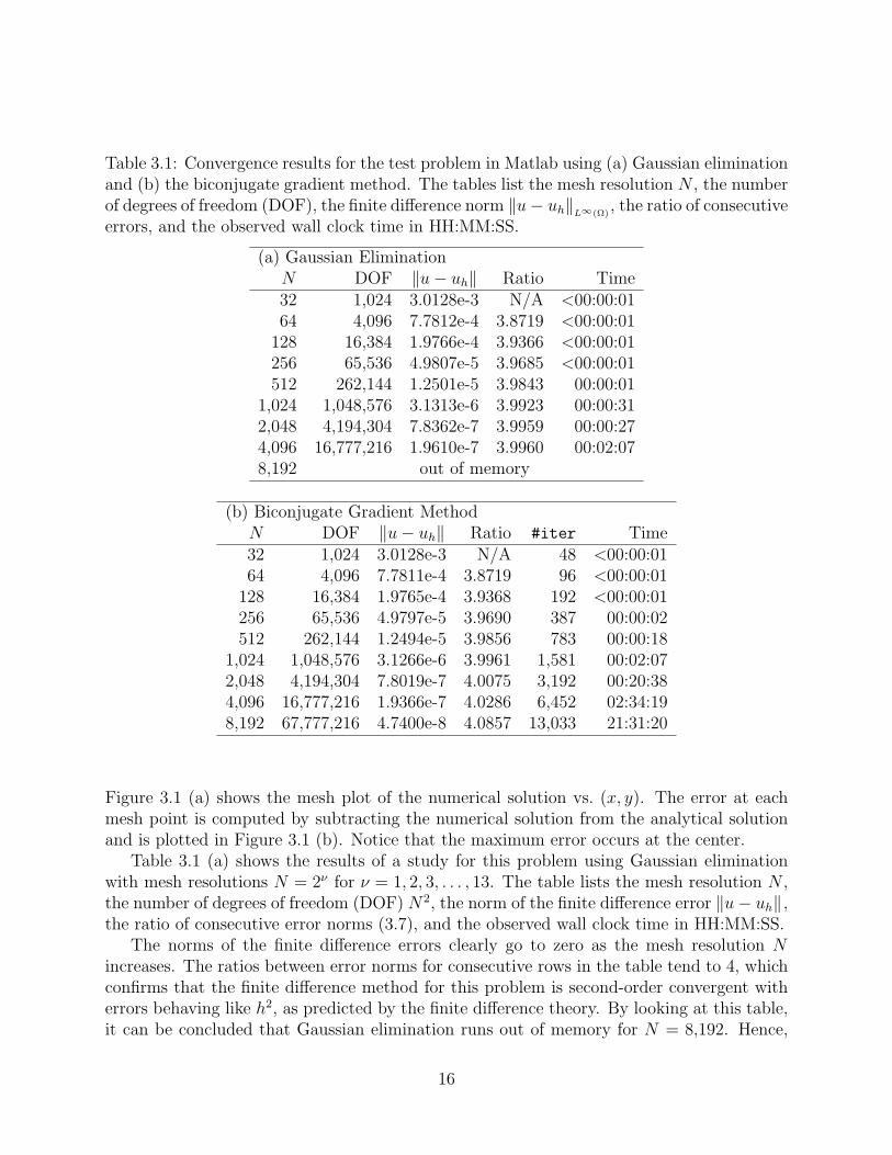
Table 3.1: Convergence results for the test problem in Matlab using (a) Gaussian eliminationand (b) the biconjugate gradient method. The tables list the mesh resolution N , the numberof degrees of freedom (DOF), the finite difference norm ‖u− uh‖L∞(Ω)

, the ratio of consecutiveerrors, and the observed wall clock time in HH:MM:SS.

(a) Gaussian EliminationN DOF ‖u− uh‖ Ratio Time32 1,024 3.0128e-3 N/A <00:00:0164 4,096 7.7812e-4 3.8719 <00:00:01

128 16,384 1.9766e-4 3.9366 <00:00:01256 65,536 4.9807e-5 3.9685 <00:00:01512 262,144 1.2501e-5 3.9843 00:00:01

1,024 1,048,576 3.1313e-6 3.9923 00:00:312,048 4,194,304 7.8362e-7 3.9959 00:00:274,096 16,777,216 1.9610e-7 3.9960 00:02:078,192 out of memory

(b) Biconjugate Gradient MethodN DOF ‖u− uh‖ Ratio #iter Time32 1,024 3.0128e-3 N/A 48 <00:00:0164 4,096 7.7811e-4 3.8719 96 <00:00:01

128 16,384 1.9765e-4 3.9368 192 <00:00:01256 65,536 4.9797e-5 3.9690 387 00:00:02512 262,144 1.2494e-5 3.9856 783 00:00:18

1,024 1,048,576 3.1266e-6 3.9961 1,581 00:02:072,048 4,194,304 7.8019e-7 4.0075 3,192 00:20:384,096 16,777,216 1.9366e-7 4.0286 6,452 02:34:198,192 67,777,216 4.7400e-8 4.0857 13,033 21:31:20

Figure 3.1 (a) shows the mesh plot of the numerical solution vs. (x, y). The error at eachmesh point is computed by subtracting the numerical solution from the analytical solutionand is plotted in Figure 3.1 (b). Notice that the maximum error occurs at the center.

Table 3.1 (a) shows the results of a study for this problem using Gaussian eliminationwith mesh resolutions N = 2ν for ν = 1, 2, 3, . . . , 13. The table lists the mesh resolution N ,the number of degrees of freedom (DOF) N2, the norm of the finite difference error ‖u− uh‖ ,the ratio of consecutive error norms (3.7), and the observed wall clock time in HH:MM:SS.

The norms of the finite difference errors clearly go to zero as the mesh resolution Nincreases. The ratios between error norms for consecutive rows in the table tend to 4, whichconfirms that the finite difference method for this problem is second-order convergent witherrors behaving like h2, as predicted by the finite difference theory. By looking at this table,it can be concluded that Gaussian elimination runs out of memory for N = 8,192. Hence,

16

we are unable to solve this problem for N larger than 4,096 via Gaussian elimination. Thisleads to the need for another method to solve larger systems. Thus, we will use an iterativemethod to solve this linear system.

3.3.2 Biconjugate Gradient Method

Now, we use the biconjugate gradient method to solve the Poisson problem [1, 9]. Thisiterative method is an alternative to using Gaussian elimination to solve a linear system andis accomplished by replacing the backslash operator by a call to the bicg function. We usethe zero vector as the initial guess and a tolerance of 10−6 on the relative residual of theiterates.

Table 3.1 (b) shows results of a study using the biconjugate gradient method with thesystem matrix A in sparse storage mode. The column #iter lists the number of iterationstaken by the iteration method to converge. The finite difference error shows the samebehavior as in Table 3.1 (a) with ratios of consecutive errors approaching 4 as for Gaussianelimination; this confirms that the tolerance on the relative residual of the iterates is tightenough.

Tables 3.1 (a) and (b) indicate that Gaussian elimination is faster than the biconjugategradient method in Matlab, whenever it does not run out of memory. For problems greaterthan 4,096, the results show that the biconjugate gradient method is able to solve for largermesh resolutions.

3.4 IDL Results

3.4.1 Gaussian Elimination

Unfortunately, there is no function or routine in IDL written to compute Gaussian elimina-tion for sparse matrices without the purchase of a separate license. With the IDL Analystlicense, IMSL_SP_LUSOL or IMSL_SP_BDSOL can be used to solve a sparse system of linearequations in various storage modes.

3.4.2 Biconjugate Gradient Method

No function or routine exists in the basic IDL license to compute the conjugate gradientmethod to solve the Poisson problem. With an extra IDL Analyst license, the routineIMSL_SP_CG is available to solve a real symmetric definite linear system using a conjugategradient method. As this routine is not available with our current license, we will usethe biconjugate gradient method available instead. The biconjugate gradient method is aniterative method which can replace the use of LU decomposition in IDL with the LINBCG

function. The zero vector is used as our initial guess. We also set the keyword ITOL=1,specifying to stop the iteration when |Ax−b|/|b| is less than the tolerance. This convergencetest with the tolerance 10−6 matches those used in the other languages.

To create the matrix A, we use three arrays holding the column and row locations, andthe specific values at those locations, in the SPRSIN function to create a sparse matrix A.

17

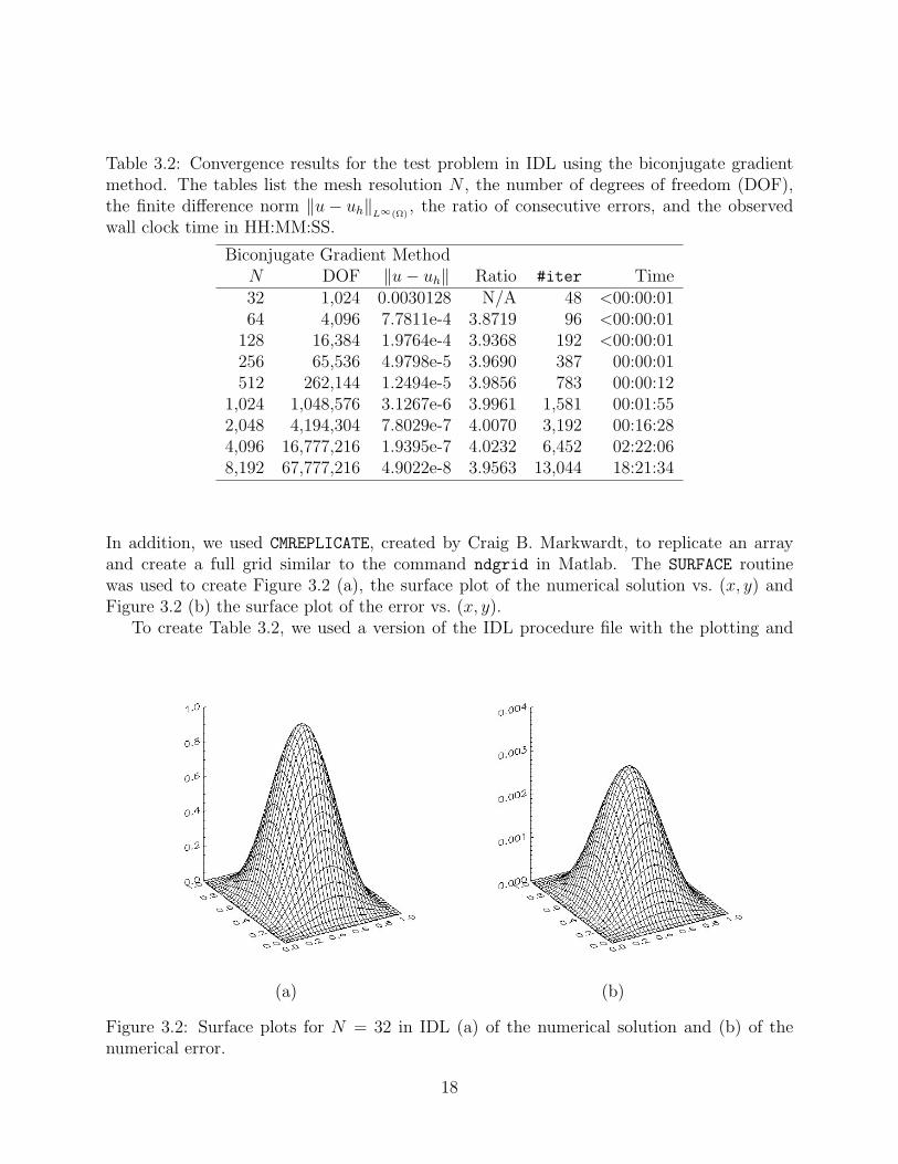
Table 3.2: Convergence results for the test problem in IDL using the biconjugate gradientmethod. The tables list the mesh resolution N , the number of degrees of freedom (DOF),the finite difference norm ‖u− uh‖L∞(Ω)

, the ratio of consecutive errors, and the observedwall clock time in HH:MM:SS.

Biconjugate Gradient MethodN DOF ‖u− uh‖ Ratio #iter Time32 1,024 0.0030128 N/A 48 <00:00:0164 4,096 7.7811e-4 3.8719 96 <00:00:01

128 16,384 1.9764e-4 3.9368 192 <00:00:01256 65,536 4.9798e-5 3.9690 387 00:00:01512 262,144 1.2494e-5 3.9856 783 00:00:12

1,024 1,048,576 3.1267e-6 3.9961 1,581 00:01:552,048 4,194,304 7.8029e-7 4.0070 3,192 00:16:284,096 16,777,216 1.9395e-7 4.0232 6,452 02:22:068,192 67,777,216 4.9022e-8 3.9563 13,044 18:21:34

In addition, we used CMREPLICATE, created by Craig B. Markwardt, to replicate an arrayand create a full grid similar to the command ndgrid in Matlab. The SURFACE routinewas used to create Figure 3.2 (a), the surface plot of the numerical solution vs. (x, y) andFigure 3.2 (b) the surface plot of the error vs. (x, y).

To create Table 3.2, we used a version of the IDL procedure file with the plotting and

(a) (b)

Figure 3.2: Surface plots for N = 32 in IDL (a) of the numerical solution and (b) of thenumerical error.

18

graphics commands commented out. This IDL biconjugate gradient method solves the prob-lem for all mesh sizes without running out of memory and is slightly faster than the Matlabresults in Table 3.1 (b).

Acknowledgments

This work was made possible with the help of Andrew Raim at the University of Maryland,Baltimore County (UMBC). The hardware used in the computational studies is part of theUMBC High Performance Computing Facility (HPCF). The facility is supported by theU.S. National Science Foundation through the MRI program (grant no. CNS–0821258) andthe SCREMS program (grant no. DMS–0821311), with additional substantial support fromthe University of Maryland, Baltimore County (UMBC). See www.umbc.edu/hpcf for moreinformation on HPCF and the projects using its resources.

References

[1] Kevin P. Allen. Efficient parallel computing for solving linear systems of equations.UMBC Review: Journal of Undergraduate Research and Creative Works, vol. 5, pp. 8–17, 2004.

[2] Dietrich Braess. Finite Elements. Cambridge University Press, third edition, 2007.

[3] Matthew Brewster and Matthias K. Gobbert. A comparative evaluation of Matlab,Octave, FreeMat, and Scilab on tara. Technical Report HPCF–2011–10, UMBC HighPerformance Computing Facility, University of Maryland, Baltimore County, 2011.

[4] James W. Demmel. Applied Numerical Linear Algebra. SIAM, 1997.

[5] Arieh Iserles. A First Course in the Numerical Analysis of Differential Equations. Cam-bridge Texts in Applied Mathematics. Cambridge University Press, second edition, 2009.

[6] Andrew M. Raim and Matthias K. Gobbert. Parallel performance studies for an el-liptic test problem on the cluster tara. Technical Report HPCF–2010–2, UMBC HighPerformance Computing Facility, University of Maryland, Baltimore County, 2010.

[7] Neeraj Sharma. A comparative study of several numerical computational packages.M.S. thesis, Department of Mathematics and Statistics, University of Maryland, Bal-timore County, 2010.

[8] Neeraj Sharma and Matthias K. Gobbert. A comparative evaluation of Matlab, Octave,FreeMat, and Scilab for research and teaching. Technical Report HPCF–2010–7, UMBCHigh Performance Computing Facility, University of Maryland, Baltimore County, 2010.

[9] David S. Watkins. Fundamentals of Matrix Computations. Wiley, third edition, 2010.

19