Identifying Vegetation from Laser Data in Structured ...stachnis/pdf/wurm13ras.pdf · Identifying...
13
Identifying Vegetation from Laser Data in Structured Outdoor Environments Kai M. Wurm, Henrik Kretzschmar, Rainer K ¨ ummerle, Cyrill Stachniss, Wolfram Burgard University of Freiburg, Dept. of Computer Science, Georges-K¨ ohler-Allee 79, 79110 Freiburg, Germany Abstract The ability to reliably detect vegetation is an important requirement for outdoor navigation with mobile robots as it enables the robot to navigate more efficiently and safely. In this paper, we present an approach to detect flat vegetation, such as grass, which cannot be identified using range measurements. This type of vegetation is typically found in structured outdoor environments such as parks or campus sites. Our approach classifies the terrain in the vicinity of the robot based on laser scans and makes use of the fact that plants exhibit specific reflection properties. It uses a support vector machine to learn a classifier for distinguishing vegetation from streets based on laser reflectivity, measured distance, and the incidence angle. In addition, it employs a vibration-based classifier to acquire training data in a self-supervised way and thus reduces manual work. Our approach has been evaluated extensively in real world experiments using several mobile robots. We furthermore evaluated it with different types of sensors and in the context of mapping, autonomous navigation, and exploration experiments. In addition, we compared it to an approach based on linear discriminant analysis. In our real world experiments, our approach yields a classification accuracy close to 100%. Keywords: Vegetation detection, laser reflectivity, self-supervised learning, terrain classification, autonomous navigation 1. Introduction Autonomous outdoor navigation is an active research field in robotics. In most outdoor navigation scenarios such as autonomous wheelchairs, surveillance robots, or transportation vehicles, the classification of terrain plays an important role as most robots have been de- signed to drive on streets and paved paths rather than on surfaces covered by grass or vegetation. Failing to stay on paved roads introduces the risk of getting stuck and additionally increases wheel slippage, which may lead to errors in the odometry. Therefore, the ability to ro- bustly detect vegetation is important for safe navigation in any of the above-mentioned situations. In this paper, we propose a novel laser-based terrain classification approach that is especially suited for de- tecting low vegetation. Such low vegetation typically occurs in structured outdoor environments such as parks or campus sites. Our approach classifies the terrain based on laser scans of the robot’s surroundings in order to allow the robot to take the classification result into ac- count during trajectory planning. Low vegetation poses a challenge for laser-based terrain classification since the variance in the measured distances is often small and thus it is hard to detect it from range measurements alone. Therefore, our approach exploits an effect that is well known from satellite image analysis: Chlorophyll, which is found in living plants, strongly reflects near-IR light [1]. Mobile robots are often equipped with laser range finders such as the popular SICK LMS scanners. These devices emit near-IR light and return the range to the object they measure along with the reflectivity of the surface. Our work formulates the detection of terrain as a classification problem that uses reflectivity, incidence angles, and the measured distances as inputs to identify whether a measured surface corresponds to vegetation. In addition to that, we provide a way to gather train- ing data in a self-supervised way and thus eliminate the cumbersome work of manually labeling training exam- ples. In this work, we evaluate two sensor setups: rotat- ing laser scanners capturing 3D pointclouds and laser scanners mounted at a fixed angle. We show that clas- sifiers can be trained in a self-supervised way using a vibration-based classification approach to label train- ing data. To integrate classification results into a rep- resentation of the environment, we apply a probabilistic mapping method similar to occupancy grid mapping [2]. Preprint submitted to Robotics and Autonomous Systems April 10, 2013
Transcript of Identifying Vegetation from Laser Data in Structured ...stachnis/pdf/wurm13ras.pdf · Identifying...

Identifying Vegetation from Laser Data in Structured Outdoor Environments
Kai M. Wurm, Henrik Kretzschmar, Rainer Kummerle, Cyrill Stachniss, Wolfram Burgard
University of Freiburg, Dept. of Computer Science, Georges-Kohler-Allee 79, 79110 Freiburg, Germany
Abstract
The ability to reliably detect vegetation is an important requirement for outdoor navigation with mobile robots as
it enables the robot to navigate more efficiently and safely. In this paper, we present an approach to detect flat
vegetation, such as grass, which cannot be identified using range measurements. This type of vegetation is typically
found in structured outdoor environments such as parks or campus sites. Our approach classifies the terrain in the
vicinity of the robot based on laser scans and makes use of the fact that plants exhibit specific reflection properties. It
uses a support vector machine to learn a classifier for distinguishing vegetation from streets based on laser reflectivity,
measured distance, and the incidence angle. In addition, it employs a vibration-based classifier to acquire training
data in a self-supervised way and thus reduces manual work. Our approach has been evaluated extensively in real
world experiments using several mobile robots. We furthermore evaluated it with different types of sensors and in the
context of mapping, autonomous navigation, and exploration experiments. In addition, we compared it to an approach
based on linear discriminant analysis. In our real world experiments, our approach yields a classification accuracy
close to 100%.
Keywords: Vegetation detection, laser reflectivity, self-supervised learning, terrain classification, autonomous
navigation
1. Introduction
Autonomous outdoor navigation is an active research
field in robotics. In most outdoor navigation scenarios
such as autonomous wheelchairs, surveillance robots,
or transportation vehicles, the classification of terrain
plays an important role as most robots have been de-
signed to drive on streets and paved paths rather than on
surfaces covered by grass or vegetation. Failing to stay
on paved roads introduces the risk of getting stuck and
additionally increases wheel slippage, which may lead
to errors in the odometry. Therefore, the ability to ro-
bustly detect vegetation is important for safe navigation
in any of the above-mentioned situations.
In this paper, we propose a novel laser-based terrain
classification approach that is especially suited for de-
tecting low vegetation. Such low vegetation typically
occurs in structured outdoor environments such as parks
or campus sites. Our approach classifies the terrain
based on laser scans of the robot’s surroundings in order
to allow the robot to take the classification result into ac-
count during trajectory planning. Low vegetation poses
a challenge for laser-based terrain classification since
the variance in the measured distances is often small
and thus it is hard to detect it from range measurements
alone. Therefore, our approach exploits an effect that is
well known from satellite image analysis: Chlorophyll,
which is found in living plants, strongly reflects near-IR
light [1]. Mobile robots are often equipped with laser
range finders such as the popular SICK LMS scanners.
These devices emit near-IR light and return the range to
the object they measure along with the reflectivity of the
surface. Our work formulates the detection of terrain as
a classification problem that uses reflectivity, incidence
angles, and the measured distances as inputs to identify
whether a measured surface corresponds to vegetation.
In addition to that, we provide a way to gather train-
ing data in a self-supervised way and thus eliminate the
cumbersome work of manually labeling training exam-
ples.
In this work, we evaluate two sensor setups: rotat-
ing laser scanners capturing 3D pointclouds and laser
scanners mounted at a fixed angle. We show that clas-
sifiers can be trained in a self-supervised way using a
vibration-based classification approach to label train-
ing data. To integrate classification results into a rep-
resentation of the environment, we apply a probabilistic
mapping method similar to occupancy grid mapping [2].
Preprint submitted to Robotics and Autonomous Systems April 10, 2013

Figure 1: A street and an area containing grass (top) and typical clas-
sification results obtained based on range differences (middle) and re-
mission values (bottom). Shown is a bird’s eye view of a 3D scan of
the area depicted at the top with a maximum range of 5 m. Whereas
points classified as street are depicted in blue, points corresponding to
vegetation are colored in green.
In our experiments, we illustrate that our approach can
be used to accurately map vegetated areas and do so
with a higher accuracy than standard techniques that are
solely based on range values (see Fig. 1). We further-
more present applications to autonomous navigation in
structured outdoor environments in which robots bene-
fit from the knowledge about the vegetation in their sur-
roundings.
This paper is organized as follows. After discussing
related work, we will briefly describe support vector
machines, which we use for classification. In Sec. 4, we
present our approach to terrain classification using laser
reflectivity. Sec. 6 describes the mapping approach used
to integrate multiple measurements of the same region.
Finally, in Sec. 9 we present the experimental results
obtained with real data and with real robots navigating
through our university campus and neighboring areas.
2. Related Work
There exist several approaches for detecting vegeta-
tion using laser measurements. Wolf et al. [3] use hid-
den Markov models to classify scans from a tilted laser
scanner into navigable (e.g., street) and non-navigable
(e.g., grass) regions. The main feature for classification
is the variance in height measurements relative to the
robot height. Other approaches analyze the distribution
of 3D endpoints in a sequence of scans [4, 5, 6]. These
algorithms are able to detect various types of obstacles
such as tree trunks, high grass, or bushes. However, flat
vegetation, such as a freshly mowed lawn, cannot be re-
liably detected using this feature alone.
It seems intuitive to use color cameras to detect vege-
tation in the environment. Manduchi, for example, uses
a combination of color and texture features to detect
grass in camera images [7]. The main drawback of us-
ing cameras is that they are sensitive to lighting condi-
tions. Shadows, for instance, can have a strong influ-
ence on the appearance of vegetation. A more robust
classifier can be derived using the Normalized Differ-
ence Vegetation Index (NDVI). This value is based on
the difference between red and near-infrared light re-
flectance and is a strong indicator for the presence of
vegetation, see [1] for a discussion on this topic. On a
mobile robot, the NDVI can be determined using a cal-
ibrated combination of a regular and an infrared cam-
era [8] or a single camera that uses a filter mask to cap-
ture both frequency bands at different positions on the
same sensor [9]. Unfortunately, such a sensor setup is
rarely available on a mobile robot and, being a passive
sensor, still depends on the presence of ambient light.
A combination of camera and laser measurements has
been used to detect vegetation in several approaches [8,
10, 11, 12]. In a combined system, Wellington et al. [12]
use the remission value of a laser scanner in addition to
density features and camera images as a classification
feature. However, they do not model the dependency
between remission, measured range, and incidence an-
gle. Probably due to this fact, they found the feature to
be only ”moderately informative”. In contrast to that,
we show in our work that remission is highly informa-
tive if it is considered jointly with the measured range
and the incidence angle of the individual laser beams.
The approach that is closest to our approach has been
proposed by Bradley et al. [8]. Vegetation is detected
using a combination of laser range measurements, regu-
lar and near-infrared cameras. Vegetation is recognized
using the NDVI computed from both camera images.
3D laser measurements of the environment are projected
into the camera images. A classifier is then trained us-
ing the vegetation feature and features from the distri-
bution of 3D endpoints. According to the authors, the
approach yields a classification accuracy of up to 95%
but requires sophisticated camera equipment. In con-
trast to such systems that consider cameras in combina-
2

tion with laser range finders or infra-red cameras, our
approach uses a laser scanner as the sole sensor. Our
system is independent of lighting conditions and can be
used on a variety of existing robot systems that are often
already equipped with a laser range finder. We evaluated
our approach in the context of detecting flat vegetation
at ranges of up to 5 m. In this setting, we achieved clas-
sification results with an accuracy of over 99% in all our
experiments.
Terrain types have also been classified using vibration
sensors on a robot [13, 14, 15, 16]. In these approaches,
the robot traverses the terrain and the induced vibration
is measured using accelerometers. The measurements
are usually analyzed in the Fourier domain. Sadhukhan
et al. [15] presented an approach based on neural net-
works. A similar approach is presented by DuPont et
al. [14]. Brooks and Iagenemma [13] use a combina-
tion of principal component analysis and linear discrim-
inant analysis to classify terrain. More recently, SVMs
have been used by Weiss et al. [16, 17]. Vibration-based
approaches typically offer highly accurate classification
results. The drawback of such methods, however, is that
only the terrain the robot is moving on can be classified
and not the terrain in front of the robot. Thus, this infor-
mation cannot be integrated well into the path planning
system of a mobile robot.
There exist previous approaches that apply self-
supervised learning to classify terrain and detect ob-
stacles. In the context of the LAGR-program (Learn-
ing Applied to Ground Robots), a number of methods
were developed that exploit terrain knowledge in the
surrounding of the robot to predict surface terrain in the
far range. These near-to-far approaches use color infor-
mation [18, 19], 3D geometry information [20], or tex-
ture information [21, 22]. Self-supervised learning was
also used by Dahlkamp et al. [23] in a vision-based road
detection system. Here, laser measurements are used to
identify nearby traversable surfaces. This information is
then used to label camera image patches in order to train
a classifier that is able to predict traversability far away
from the robot. In our approach, we adopt the idea of
self-supervision to generate labeled training data. We
apply a vibration-based classifier to label laser mea-
surements recorded by the robot. This labeled dataset
is then used to train a laser-based vegetation classifier.
Both classifiers used in our approach have been imple-
mented using support vector machines, which will be
introduced in the following section.
This paper extends our previously published confer-
ence paper [24]. First, we provide an extended discus-
sion and evaluation including new experiments. Several
different sensor types are evaluated and additional large-
scale, autonomous navigation and mapping experiments
are presented. Second, we provide means for compu-
tationally efficient classification so that terrain classifi-
cation can be carried out on low-powered devices with
limited computational resources, which was not directly
possible with our previously presented system.
3. Support Vector Machines
The support vector machine (SVM) is a kernel-based
learning method which is widely used for classification
and regression problems [25]. The SVM learns a hy-
perplane in a higher-dimensional feature space. Two
classes of data points are separated by a hyperplane so
that the margin between training points and the plane is
maximized:
maxw∈H,b∈R
minxi∈D{||x − xi|| | x ∈ H, 〈w, x〉 + b = 0}, (1)
where H is some dot product space, xi ∈ D are train-
ing points, and w is a weighting vector. The following
decision function is used to determine the class label y:
f (x) = 〈w, x〉 + b (2)
y = sgn( f (x)) (3)
The hyperplane can be constructed by solving a
quadratic programming problem. To separate nonlin-
ear classes, the so-called kernel trick is applied. The
training data is first mapped into a higher-dimensional
feature space using a kernel function. A separating hy-
perplane is then constructed in this features space which
yields a nonlinear decision boundary in the input space.
In practice, the Gaussian radial basis function (RBF) is
often used as a kernel function. It is given by
k(x, x′) = exp
(
−(x − x′)2
2l2
)
, (4)
where l is the so-called length-scale parameter.
There exist derivatives of the basic SVM-formulation
that are robust against occasional mislabeled training
points. Among those, C-SVM is a popular method that
uses a soft margin. An additional parameter commonly
denoted as C adjusts the trade-off between maximizing
the margin and minimizing the training error. Through-
out this work, we use the C-SVM implementation of
LibSVM [26].
3.1. Class Probabilities
The decision function of support vector machines, as
given in Eq. 3, yields a class label y which is not a prob-
ability: y is either -1 or 1. In many cases, however, it
3
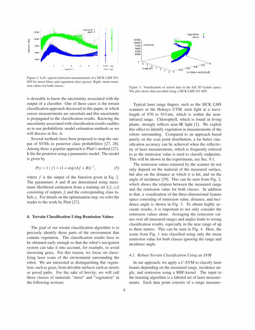
Figure 2: Left: typical remission measurements of a SICK LMS 291-
S05 for street (blue) and vegetation class (green). Right: mean remis-
sion values for both classes.
is desirable to know the uncertainty associated with the
output of a classifier. One of these cases is the terrain
classification approach discussed in this paper, in which
sensor measurements are uncertain and this uncertainty
is propagated to the classification results. Knowing the
uncertainty associated with classification results enables
us to use probabilistic model estimation methods as we
will discuss in Sec. 6.
Several methods have been proposed to map the out-
put of SVMs to posterior class probabilities [27, 28].
Among those a popular approach is Platt’s method [27].
It fits the posterior using a parametric model. The model
is given by
P(y = 1 | f ) = (1 + exp (A f + B))−1, (5)
where f is the output of the function given in Eq. 2.
The parameters A and B are determined using maxi-
mum likelihood estimation from a training set {( fi, yi)}
consisting of outputs fi and the corresponding class la-
bels yi. For details on the optimization step, we refer the
reader to the work by Platt [27].
4. Terrain Classification Using Remission Values
The goal of our terrain classification algorithm is to
precisely identify those parts of the environment that
contain vegetation. The classification results have to
be obtained early enough so that the robot’s navigation
system can take it into account, for example, to avoid
traversing grass. For this reason, we focus on classi-
fying laser scans of the environment surrounding the
robot. We are interested in distinguishing flat vegeta-
tion, such as grass, from drivable surfaces such as streets
or paved paths. For the sake of brevity, we will call
those classes of materials ”street” and ”vegetation” in
the following sections.
Figure 3: Visualization of sensor data in the full 3D feature space.
The plot shows data recorded using a SICK LMS 291-S05.
Typical laser range fingers, such as the SICK LMS
scanners or the Hokuyo UTM, emit light at a wave-
length of 870 to 915 nm, which is within the near-
infrared range. Chlorophyll, which is found in living
plants, strongly reflects near-IR light [1]. We exploit
this effect to identify vegetation in measurements of the
robots surrounding. Compared to an approach based
purely on the scan point distribution, a far better clas-
sification accuracy can be achieved when the reflectiv-
ity of laser measurements, which is frequently referred
to as the remission value is used to classify endpoints.
This will be shown in the experiments, see Sec. 9.1.
The remission values returned by the scanner do not
only depend on the material of the measured surface,
but also on the distance at which it is hit, and on the
angle of incidence [29]. This can be seen from Fig. 2,
which shows the relation between the measured range
and the remission value for both classes. In addition
to that, a visualization of the three-dimensional feature
space consisting of remission value, distance, and inci-
dence angle is shown in Fig. 3. To obtain highly ac-
curate results, it is important to not only consider the
remission values alone. Averaging the remission val-
ues over all measured ranges and angles leads to wrong
classification results, especially in the near range of up
to three meters. This can be seen in Fig. 4. Here, the
scene from Fig. 1 was classified using only the mean
remission value for both classes ignoring the range and
incidence angle.
4.1. Robust Terrain Classification Using an SVM
In our approach, we apply a C-SVM to classify laser
beams depending on the measured range, incidence an-
gle, and remission using a RBF-kernel. The input to
the learning algorithm is a labeled set of laser measure-
ments. Each data point consists of a range measure-
4
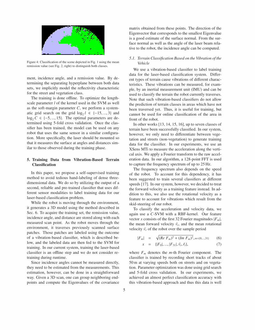
Figure 4: Classification of the scene depicted in Fig. 1 using the mean
remission value (see Fig. 2, right) to distinguish both classes.
ment, incidence angle, and a remission value. By de-
termining the separating hyperplane between both data
sets, we implicitly model the reflectivity characteristic
for the street and vegetation class.
The training is done offline. To optimize the length-
scale parameter l of the kernel used in the SVM as well
as the soft-margin parameter C, we perform a system-
atic grid search on the grid log2 l ∈ {−15, ..., 3} and
log2 C ∈ {−5, ..., 15}. The optimal parameters are de-
termined using 5-fold cross validation. Once the clas-
sifier has been trained, the model can be used on any
robot that uses the same sensor in a similar configura-
tion. More specifically, the laser should be mounted so
that it measures the surface at angles and distances sim-
ilar to those observed during the training phase.
5. Training Data from Vibration-Based Terrain
Classification
In this paper, we propose a self-supervised training
method to avoid tedious hand-labeling of dense three-
dimensional data. We do so by utilizing the output of a
second, reliable and pre-trained classifier that uses dif-
ferent sensor modalities to label training data for our
laser-based classification problem.
While the robot is moving through the environment,
it generates a 3D model using the method described in
Sec. 6. To acquire the training set, the remission value,
incidence angle, and distance are stored along with each
measured scan point. As the robot moves through the
environment, it traverses previously scanned surface
patches. Those patches are labeled using the outcome
of a vibration-based classifier, which is described be-
low, and the labeled data are then fed to the SVM for
training. In our current system, training the laser-based
classifier is an offline step and we do not consider re-
training during runtime.
Since incidence angles cannot be measured directly,
they need to be estimated from the measurements. This
estimation, however, can be done in a straightforward
way. Given a 3D scan, one can group neighboring end-
points and compute the Eigenvalues of the covariance
matrix obtained from these points. The direction of the
Eigenvector that corresponds to the smallest Eigenvalue
is a good estimate of the surface normal. From the sur-
face normal as well as the angle of the laser beam rela-
tive to the robot, the incidence angle can be computed.
5.1. Terrain Classification Based on the Vibration of the
Vehicle
We use a vibration-based classifier to label training
data for the laser-based classification system. Differ-
ent types of terrain cause vibrations of different charac-
teristics. These vibrations can be measured, for exam-
ple, by an inertial measurement unit (IMU) and can be
used to classify the terrain the robot currently traverses.
Note that such vibration-based classifiers do not allow
the prediction of terrain classes in areas which have not
been traversed yet. Thus, it is useful for training, but
cannot be used for online classification of the area in
front of the robot.
In other works [13, 14, 15, 16], up to seven classes of
terrain have been successfully classified. In our system,
however, we only need to differentiate between vege-
tation and streets (non-vegetation) to generate training
data for the classifier. In our experiments, we use an
XSens MTi to measure the acceleration along the verti-
cal axis. We apply a Fourier transform to the raw accel-
eration data. In our algorithm, a 128-point FFT is used
to capture the frequency spectrum of up to 25 Hz.
The frequency spectrum also depends on the speed
of the robot. To account for this dependency, it has
been suggested to train several classifiers at different
speeds [17]. In our system, however, we decided to treat
the forward velocity as a training feature instead. In ad-
dition to this, we also use the rotational velocity as a
feature to account for vibrations which result from the
skid-steering of our robot.
To classify the acceleration and velocity data, we
again use a C-SVM with a RBF-kernel. Our feature
vector x consists of the first 32 Fourier magnitudes |Fm|,
the mean forward velocity vt, and the mean rotational
velocity vr of the robot over the sample period
|Fm| =√
(Re Fm)2 + (Im Fm)2,m ∈{0,...,31} (6)
x = {|F0|, ..., |F31|, vt, rt}, (7)
where Fm denotes the m-th Fourier component. The
classifier is trained by recording short tracks of about
50 m at varying speeds both on streets and on vegeta-
tion. Parameter optimization was done using grid search
and 5-fold cross validation. In our experiments, we
achieved an almost perfect classification accuracy with
this vibration-based approach and thus this data is well
5

Figure 5: Visualization of a 3D model with vegetation highlighted in
green.
suited to label the training data for the laser-based clas-
sification.
6. Mapping Vegetation
We use multi-level surface maps [30] to model the
environment. This representation uses a 2D grid and in
each cell stores a set of patches representing individual
surfaces at different heights. In our approach, we main-
tain the probability of vegetation for each surface patch.
Let P(vi) denote this probability for patch i. In general,
surface patches will be observed multiple times. For
this reason, we need to probabilistically combine results
from several measurements. In this way, the uncertainty
in classification is explicitly taken into account.
Let zt be a laser measurement at time t. Analogous
to Moravec [2], we obtain an update rule for P(vi | z1:t).
First, we apply Bayes’ rule and obtain
P(vi | z1:t) =P(zt | v
i, z1:t−1)P(vi | z1:t−1)
P(zt | z1:t−1). (8)
We then compute the ratio
P(vi | z1:t)
P(¬vi | z1:t)=
P(zt | vi, z1:t−1)
P(zt | ¬vi, z1:t−1)
P(vi | z1:t−1)
P(¬vi | z1:t−1). (9)
Similarly, we obtain
P(vi | zt)
P(¬vi | zt)=
P(zt | vi)
P(zt | ¬vi)
P(vi)
P(¬vi),
which can be transformed to
P(zt | vi)
P(zt | ¬vi)=
P(vi | zt)
P(¬vi | zt)
P(¬vi)
P(vi). (10)
Applying the Markov assumption that the current obser-
vation is independent of previous observations given we
know that a patch contains vegetation gives
P(zt | vi, z1:t−1) = P(zt | v
i), (11)
Figure 6: Sensors used in the evaluation.
and utilizing the fact that P(¬vi) = 1 − P(vi), we obtain
P(vi | z1:t)
1 − P(vi | z1:t)=
P(vi | zt)
1 − P(vi | zt)
P(vi | z1:t−1)
1 − P(vi | z1:t−1)
1 − P(vi)
P(vi). (12)
This equation can be transformed into the following up-
date formula:
P(vi | z1:t) =[
1 +1 − P(vi | zt)
P(vi | zt)
1 − P(vi | z1:t−1)
P(vi | z1:t−1)
P(vi)
1 − P(vi)
]−1
(13)
To perform the update step, we need an inverse sensor
model P(vi | z). This, however, can directly be obtained
from the estimated class probabilities of the classifier.
During the training phase, we apply Platt’s method as
discussed in Sec. 3.1. The posterior class probabili-
ties computed using Eq. 5 constitute an inverse sensor
model and in this way the uncertainty in classification is
explicitly taken into account.
The prior probability of a patch to contain vegetation
P(vi) clearly depends on the environment that the robot
is operating in. In our system, it was set to 0.5 to not
preference any class. This seems reasonable in an envi-
ronment such as the one depicted in Fig. 12 but can be
adapted if this is needed.
7. Comparison of Different Sensors
Most laser range finders that are used on mobile
robots are able to provide range and remission infor-
mation and all of these sensors measure surfaces using
near-infrared light. Thus our approach can be applied to
data from any such sensor as long as it provides remis-
sion values. We evaluated three different laser scanners
under comparable conditions. The sensors we evaluated
were the SICK LMS 291-S05, the SICK LMS 151, and
6
Figure 7: Comparison of remission values of a SICK LMS 291 (top),
SICK LMS 151 (middle), and a Hokuyo UTM 30LX (bottom). Please
note that these are projections of the full three-dimensional data sets
since incidence angles are not shown.
the Hokuyo UTM 30LX (see Fig. 6). Each scanner was
mounted on a mobile robot at a fixed angle of 70 degrees
relative to the ground and was mounted at a height of
approximately 0.6 m. We recorded range and remission
data by moving the robot so that the sensors were swept
over a street and areas that contained vegetation.1
Example data from the sensors of both classes (pro-
jected into the two dimensional space for a better visu-
alization) is depicted in the plots in Fig. 7. It can be seen
that all sensors report a considerably higher reflectivity
for vegetation than for the street. In this projection, the
LMS 291 offers the best separation of the classes, es-
1Data available at:
http://ais.informatik.uni-freiburg.de/remission-data
Figure 8: Left: remission values of a SICK LMS 151 measuring veg-
etation, light tiles, and an asphalt street. Right: examples of the mea-
sured surfaces.
pecially in the near range, followed by the LMS 151.
Using the Hokuyo UTM, measurements of both classes
are not well separated in the near range of up to approx-
imately one meter.
It is worth mentioning that the measured difference
in the reflectivity is not due to the lighter color of grass
compared to a dark street. In Figure 8, remission data
from a surface covered with light tiles is shown. These
tiles exhibit a visual brightness similar to grass. It can be
seen that the measured infrared reflectivities are higher
than those of an asphalt street but still considerably
lower than those of vegetation.
From the examples shown above, one can see that all
three sensors can be used for vegetation detection, but
the classification accuracy may vary. Depending on the
type of sensor, a minimum distance to the ground should
be kept for reliable results since in this area, it may be
challenging to separate the classes.
8. Classification for Resource Constrained Systems
On systems with limited computational resources,
such as embedded systems, the SVM classifier can be
computationally too demanding to be used online. The
computational complexity of the SVM results from the
evaluation of the kernel and the potentially high num-
ber of support vectors that are needed to appropriately
separate the classes. For each laser scan, assuming a
frequency of 36 Hz and 180 laser beams per scan, 6,480
classifications per second need to be performed.
To reduce the computational complexity, we apply
linear discriminant analysis [31] to project the three-
dimensional feature space (range, incidence angle, re-
mission) down to one dimension such that the two
classes are best separated. Given this projection, we
can then apply an efficient linear classifier to separate
the classes and to compute class probabilities for laser
7

data points
of class 2
axis selected by LDA
of class 1
data points
Figure 9: Reduction from R2 to R using LDA. LDA seeks to separate
the two classes (illustrated by green and blue) as well as possible.
measurements based on a Gaussian assumption. The
individual steps are explained in the remainder of this
section.
8.1. Linear Discriminant Analysis
Linear discriminant analysis (LDA) is a supervised
dimensionality reduction technique that is similar to
PCA. In contrast to PCA, LDA allows to exploit the la-
bels of the datapoints and seeks to estimate a reduced
space so that the classes are best separated. Reducing
the space to a one-dimensional one, then allows to sep-
arate the classes with a naive Bayesian classifier. An
illustration of a reduction from R2 to R is shown in Fig-
ure 9. We refer to Alpaydin [31] for more details.
LDA works as follows. Let K be the number of
classes Ck and xi the d-dimensional inputs, here K = 2
and d = 3. Let furthermore t be the dimensionality of
the target space, in our experiments we found a one-
dimensional target space to be sufficient. The objective
is to find a d× t matrix W so that vi = WT xi with vi ∈ Rt
and so that the classes Ck are separated best in terms of
distances between the vi.
Let rk,i be an indicator variable with rk,i = 1 if xi ∈ Ck
and 0 otherwise. Let mk be the mean of d-dimensional
vectors xi ∈ Ck. Then, the so-called total within-scatter
matrix is given by
S W =
K∑
k=1
∑
i
rk,i(xi − mk)(xi − mk)T
, (14)
and the between-class scatter matrix by
S B =
K∑
k=1
∑
i
rk,i
(mk − m)(mk − m)T, (15)
with
m =1
K
K∑
k=1
mk. (16)
Now let us consider the scatter matrices after projection
using W. The between-class scatter matrix after projec-
tion is WT S BW, and the within-scatter matrix accord-
ingly, both are t×t dimensional. The goal is to determine
W in a way that the means of the classes WT mk are as
far apart from each other as possible while the spread of
their individual projected class samples is small. Simi-
lar to covariance matrices, the determinant of a scatter
matrix characterizes the spread and it is computed as the
product of the eigenvalues specifying the variance along
the eigenvectors. Thus we aim at finding the matrix W
that maximizes
J(W) =|WT S BW |
|WT S WW |. (17)
The largest eigenvectors of S −1W
S B are the solution to
this problem.
8.2. Classification Using Linear Discriminant Analysis
Given the projection computed by LDA, we use an
efficient linear classifier to compute class probabilities
for laser measurements. For each class Ck, our method
fits a Gaussian distribution, p(x | Ck), to the one-
dimensional data using maximum likelihood estimation.
Using Bayes’ theorem, we obtain the posterior probabil-
ities
p(Ck | x) =p(x | Ck)p(Ck)
∑
i p(x | Ci)p(Ci), (18)
where p(Ci) is the class prior for class Ci. Since in our
case, we have two classes and a uniform prior, this turns
into
p(Ck | x) =p(x | Ck)
p(x | C1) + p(x | C2), (19)
with k ∈ {1, 2}, referring to the classes vegetation and
streets. Note that this simplified classification approach
is significantly faster than the SVM, but it is also less
powerful. Our evaluation in Sec. 9.6 shows that the re-
sulting error depends on the type of sensor and the mea-
surement range. In our experiments, we observed that
the precision dropped from 99% down to 96% in the
worst case compared to the SVM-based classifier while
LDA-based system was around two orders of magnitude
faster than the SVM in our settings.
9. Evaluation
Our approach has been implemented and evaluated
in several experiments. The experiments are designed
to demonstrate that our approach improves navigation
8

Figure 10: Robots used in our experiments. Left: An ActiveMedia
Powerbot (yellow) and a Pioneer2 AT (red). Right: the EUROPA
platform.
in structured outdoor environments by enabling robots
to reliably detect vegetation.
We used three different robot systems (see Fig. 10).
The self-supervised learning approach is evaluated us-
ing an ActivMedia Pioneer2 AT, which is able to tra-
verse low vegetation. For mapping large environments
and for an autonomous driving experiment, we use
an ActivMedia Powerbot platform. This robot cannot
safely traverse grass since its castor wheels will block
the robot due to its weight. Both robots are equipped
with SICK LMS S291-S05 laser scanners on pan-tilt
units. In addition to that, the Pioneer robot carries
an XSens MTi IMU to measure vibrations. Three-
dimensional scans are gathered by tilting the laser scan-
ner from 50 degrees upwards to 30 degrees downwards.
To evaluate classification on a SICK LMS 151 sensor
mounted at a fixed angle, we use the custom-made EU-
ROPA robot platform depicted in Fig. 10 (right). Just as
the Powerbot, this platform cannot safely traverse vege-
tation.
We limit the classification to scans with a range
smaller than 5.0 meters. The approach itself is not lim-
ited in range. However, due to the coarse angular reso-
lution of the laser scanners and a low mounting height
of the sensor relative to the ground (approximately 0.5-
0.6 m), long range data is too sparse both to gather train-
ing data and to reliably detect drivable surfaces and ob-
stacles.
In our current implementation, structures that can be
reliably detected as obstacles are not considered in the
classification step. This decision is made based on the
height difference between potential obstacles and their
surrounding. In our experiments, we set this threshold
to 0.1 m. Such obstacles are not traversable regardless
of whether they are covered by vegetation or not. Note
that the classification approach itself would even work
on arbitrary surfaces given the approximate knowledge
of the surface normal.
9.1. Comparison to Vegetation Detection Using Range
Differences
In a first experiment, we implemented a vegetation
detection algorithm based purely on the range differ-
ences of neighboring laser measurements similar to the
one proposed by Wolf et al. [3]. This method is only
used as a comparison with our proposed classification
approach. Three-dimensional data are acquired by gath-
ering a sweep of 2D scans. For each 2D scan, the 2D
endpoints pi = 〈xi, yi〉 are computed from the range and
angle measurements 〈ri, αi〉. A local feature di is then
determined for every scan point
di = xi − xi−1. (20)
This feature captures the local roughness of the terrain.
To cope with flat but tilted surfaces, we classify scans
based on the absolute difference in di between adjacent
range measurements, as suggested in [11]. Furthermore,
we also use the measured range as a training feature to
account for the varying data density from near to far
scans. We use an SVM to train a classifier based on
these features.
In our experiments, we achieve a classification ac-
curacy of about 75% using the described method. An
example of the classification results can be seen in
Fig. 1. Similar results have been reported by other re-
searchers [8]. While this result certainly shows that
geometric features are useful to detect vegetation, we
will show that a substantially higher accuracy can be
achieved in case of detecting flat vegetation in the sur-
rounding of the robot.
9.2. Self-Supervised Learning
To train our remission-based classifier, we joysticked
the Pioneer AT robot through an outdoor environment
consisting of a street and an area covered with grass.
We acquired 3D scans approximately every 4 m. While
the robot was driving, the IMU measured the vibration
of the robot. To correct odometry errors of the robot,
we employed a 2D SLAM approach [32] and its freely
available implementation [33] in combination with 3D
scan-matching. We trained our classifier using the self-
supervised approach described in Sec. 4.1. The train-
ing set is visualized in Fig. 11a. The data recorded at
the border region between street and vegetation were ig-
nored since the precise location of the border cannot be
determined using the vibration sensor. The model for
the laser-based classifier was trained using 19,989 veg-
etation and 11,248 street samples.
To evaluate the precision of the classifier, we
recorded separate test data at a different location (see
9
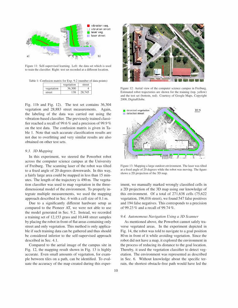
Figure 11: Self-supervised learning. Left: the data set which is used
to train the classifier. Right: test set recorded at a different location.
Table 1: Confusion matrix for Exp. 9.2 (number of data points)
vegetation street
vegetation 36,300 4
street 138 28,745
Fig. 11b and Fig. 12). The test set contains 36,304
vegetation and 28,883 street measurements. Again,
the labeling of the data was carried out using the
vibration-based classifier. The previously trained classi-
fier reached a recall of 99.6 % and a precision of 99.9 %
on the test data. The confusion matrix is given in Ta-
ble 1. Note that such accurate classification results are
not due to overfitting and very similar results are also
obtained on other test sets.
9.3. 3D Mapping
In this experiment, we steered the Powerbot robot
across the computer science campus at the University
of Freiburg. The scanning laser of the robot was tilted
to a fixed angle of 20 degrees downwards. In this way,
a fairly large area could be mapped in less than 15 min-
utes. The length of the trajectory is 490 m. The vegeta-
tion classifier was used to map vegetation in the three-
dimensional model of the environment. To properly in-
tegrate multiple measurements, we used the mapping
approach described in Sec. 6 with a cell size of 0.1 m.
Due to a significantly different hardware setup as
compared to the Pioneer AT, we were not able to use
the model generated in Sec. 9.2. Instead, we recorded
a training set of 12,153 grass and 10,448 street samples
by placing the robot in front of flat areas containing only
street and only vegetation. This method is only applica-
ble if such training data can be gathered and thus should
be considered inferior to the self-supervised approach
described in Sec. 4.1.
Compared to the aerial image of the campus site in
Fig. 12, the mapping result shown in Fig. 13 is highly
accurate. Even small amounts of vegetation, for exam-
ple between tiles on a path, can be identified. To eval-
uate the accuracy of the map created during this exper-
Figure 12: Aerial view of the computer science campus in Freiburg.
Estimated robot trajectories are shown for the training (top, yellow)
and the test set (bottom, red). Courtesy of Google Maps, Copyright
2008, DigitalGlobe.
Figure 13: Mapping a large outdoor environment. The laser was tilted
at a fixed angle of 20 degrees while the robot was moving. The figure
shows a 2D projection of the 3D map.
iment, we manually marked wrongly classified cells in
a 2D projection of the 3D map using our knowledge of
this environment. Of a total of 271,638 cells (75,622
vegetation, 196,016 street), we found 547 false positives
and 194 false negatives. This corresponds to a precision
of 99.23 % and a recall of 99.74 %.
9.4. Autonomous Navigation Using a 3D Scanner
As mentioned above, the Powerbot cannot safely tra-
verse vegetated areas. In the experiment depicted in
Fig. 14, the robot was told to navigate to a goal position
80 m in front of it while avoiding vegetation. Since the
robot did not have a map, it explored the environment in
the process of reducing its distance to the goal location.
Thereby, it used the vegetation classifier to detect veg-
etation. The environment was represented as described
in Sec. 6. Without knowledge about the specific ter-
rain, the shortest obstacle-free path would have led the
10

Figure 14: Autonomous navigation experiment. Although the shortest
obstacle-free path from the start to the goal position led over grass,
the robot reliably avoided the vegetated areas by using our vegetation
classifier and traveled over the paved streets to reach its goal.
robot across a large area containing grass. By consider-
ing the classification results in the path costs, however,
the planner chose a safe trajectory over the street.
9.5. Autonomous Navigation Using a Fixed-Angle Sen-
sor
To obtain a map of the campus surroundings, the
custom-made EUROPA platform depicted in Fig. 10
(right), equipped with a SICK LMS 151 mounted at
a fixed angle, was steered along a 7,500 m trajectory
through the campus and parts of Freiburg. Addition-
ally, the data collected by a horizontally mounted range
finder are considered for building a 2D occupancy grid.
The mapped area combines the computer science cam-
pus, urban areas, and the park area of a Freiburg Uni-
versity hospital.
We trained the classifier using data recorded by plac-
ing the robot in front of grassland and on a street. Using
the collected data, our mapping approach presented in
Sec. 6 was able to obtain a map in which the drivable
street and non-traversable vegetation were accurately la-
beled. Fig. 15 visualizes the resulting map which was
used to carry out an autonomous navigation experiment.
At the beginning of the experiment, the robot was lo-
cated on the campus in the top left of the map. The
goal location was within the park area in the lower right
part of the map. By taking into account the classifica-
tion result of our approach, the robot was able to plan a
feasible and safe path towards the goal location. While
navigating along the planned path the robot used its hor-
izontally mounted range finder to localize itself given
the occupancy map. The robot autonomously traveled
a total distance of approximately 1,120 m and success-
fully reached the goal location. The trajectory that the
robot followed is shown as a red line in Fig. 15. Without
Figure 15: Autonomous navigation experiment. The robot planned a
path on a map annotated by our approach. The robot autonomously
traveled a distance of approximately 1,120 m. Each black rectangle
shows a magnified view of a particular area of the environment.
classifying the vegetation the shortest path would have
led partially across large areas covered with vegetation
which induces a high risk of getting stuck.
9.6. Resource-Friendly Classification with Linear Dis-
criminant Analysis
In this section, we compare the accuracy of the SVM
and linear discriminant analysis. The LDA approach
is less computationally demanding and thus is useful
for resource-constraint systems or for robots that run a
fairly large number of processes. We evaluated both ap-
proaches on data that we recorded with three different
laser scanners, i.e., SICK LMS 151, SICK LMS 291,
and Hokuyo UTM 30LX.
We divided each dataset into a training dataset con-
taining 2,000 randomly sampled data points and a test
dataset containing all the remaining data points. The re-
sults are depicted in Tab. 2. Using the LDA approach
11
Table 2: Comparison between the SVM-based and the LDA-based
classifiersprecision recall precision recall
(SVM) (SVM) (LDA) (LDA)
LMS 151 99.7% 100% 99.1% 99.8%
LMS 291 99.9% 100% 99.4% 100%
UTM 99.9% 99.9% 96.3% 99.8%
on the SICK LMS 151 dataset resulted in a recall of
99.1% and a precision of 99.8%, whereas the SVM-
based classifier gave a recall of 99.7% and a precision of
100.0%. Using the SICK LMS 291 dataset, the LDA-
based approach yielded a recall of 99.4% and a preci-
sion of 100.0%, whereas the use of the SVM resulted in
a recall of 99.9% and in a precision of 100.0%. When
applied to the Hokuyo UTM 30LX dataset, the LDA-
based approach reached a recall of 96.3% and a preci-
sion of 99.8%, while the SVM-based classifier gave a
recall of 99.9% and a precision of 99.9%.
These results show that both approaches achieve a
highly accurate classification. In all cases, the SVM-
based approach outperforms the LDA-based method.
The relative difference, however, is small. When an-
alyzing the errors, we observed that most of the mis-
classification of the LDA-based classifier occur at range
measurements below 2 m. This means that the system
potentially makes poor predictions when classifying ar-
eas close to the robot, which may cause the navigation
system to stop the vehicle to avoid potential obstacles.
Therefore, the highly accurate results of the SVM-based
system are preferable for online navigation tasks.
We also compared the runtimes of the SVM and the
LDA-based approach. In our experiments, the LDA-
based approach was around 400 times faster than the
classification using the support vector machine on a reg-
ular desktop computer. The SVM used 21 support vec-
tors to separate the training data in this evaluation.
10. Conclusion
In this paper, we presented a novel approach to veg-
etation detection that uses the remission values of laser
scanners. Laser remission values depend on the surface
reflectivity as well as on the distance and the angle of
incidence. This dependency has not been considered by
previous methods that detect vegetation. Our approach
trains a classifier based on individual laser measure-
ments consisting of the remission value, the distance to
the surface, and the angle of incidence. Our method
is able to distinguish vegetation from drivable surfaces
such as streets. To predict the terrain type, we use a
support vector machine (SVM). We avoid the need to
label training data manually by labeling sets of example
measurements in a self-supervised fashion by means of
a pre-trained vibration-based terrain classifier. In addi-
tion to the system based on support vector machines,
we presented a classification approach based on linear
discriminant analysis (LDA). This system is around 400
times faster than the SVM-based approach and is es-
pecially designed for robots with limited computational
resources. Both approaches have been implemented and
evaluated in various real-world experiments. Our ex-
periments show that the SVM-based approach is able
to accurately detect low, grass-like vegetation with an
accuracy of close to 100%. The classification method
based on LDA achieves accurate predictions, but in our
experiments they were up to 4% worse than results of
the SVM-based approach. In further experiments, we
demonstrated that autonomous robots are able to navi-
gate efficiently and safely in structured outdoor environ-
ments using our terrain classification method.
11. Future Work
In our experiments, training and testing data were
collected on clear days by measuring try surfaces. Rain
water or snow might affect the reflectivity – to what ex-
tent water affects classification results and how this can
be detected is subject to future work.
The experiments presented in this paper were per-
formed in early spring and in summer. Our approach
was able to detect grass that was yellowed from being
covered by snow in the preceding days. Future work
could provide a more thorough evaluation of the impact
of reduced chlorophyll on laser reflectivity.
The vibration-based classifier provided accurate
training data in our experiments. If the training signal
contained considerable noise, it might be possible to use
the probabilistic output of the SVM-classifier to avoid
uncertain training data.
Acknowledgment
This work has partly been supported by the Ger-
man Research Foundation (DFG) under contract num-
ber SFB/TR-8 (A3) and by the European Commission
under contract number FP7-231888-EUROPA and FP7-
248873-RADHAR.
References
[1] R. Myneni, F. Hall, P. Sellers, A. Marshak, The interpretation of
spectral vegetation indexes, IEEE Transactions on Geoscience
and Remote Sensing 33 (2) (1995) 481–486.
12

[2] H. Moravec, Sensor fusion in certainty grids for mobile robots,
AI Magazine (1988) 61–74.
[3] D. Wolf, G. Sukhatme, D. Fox, W. Burgard, Autonomous ter-
rain mapping and classification using hidden markov models, in:
Proc. of the IEEE Int. Conf. on Robotics & Automation (ICRA),
2005.
[4] M. Hebert, N. Vandapel, Terrain classification techniques from
ladar data for autonomous navigation, in: Proc. of the Collab-
orative Technology Alliances conference, College Park, MD.,
2003.
[5] J.-F. Lalonde, N. Vandapel, D. Huber, M. Hebert, Natural ter-
rain classification using three-dimensional ladar data for ground
robot mobility, Journal of Field Robotics 23 (10) (2006) 839 –
861.
[6] J. Macedo, R. Manduchi, L. Matthies, Ladar-based discrimi-
nation of grass from obstacles for autonomous navigation, in:
ISER 2000: Experimental Robotics VII, London, UK, 2001.
[7] R. Manduchi, Bayesian fusion of color and texture segmenta-
tions, in: Proc. of the Int. Conf. on Computer Vision (ICCV),
1999, p. 956.
[8] D. Bradley, R. Unnikrishnan, J. Bagnell, Vegetation detection
for driving in complex environments, in: Proc. of the IEEE
Int. Conf. on Robotics & Automation (ICRA), 2007.
[9] B. Zhao, L. Tian, T. Ahamed, Real-time ndvi measurement us-
ing a low-cost panchromatic sensor for a mobile robot platform,
Environment Control in Biology 48 (2) (2010) 73–79.
[10] B. Douillard, D. Fox, F. Ramos, Laser and vision based outdoor
object mapping, in: Proceedings of Robotics: Science and Sys-
tems IV, Zurich, Switzerland, 2008.
[11] R. Manduchi, A. Castano, A. Talukder, L.Matthies, Obstacle de-
tection and terrain classification for autonomous off-road navi-
gation, Autonomous Robots, 18 (2003) 81–102.
[12] C. Wellington, A. Courville, A. Stentz, A generative model of
terrain for autonomous navigation in vegetation, International
Journal of Robotics Research 25 (12) (2006) 1287 – 1304.
[13] C. Brooks, K. Iagnemma, S. Dubowsky, Vibration-based terrain
analysis for mobile robots, in: Proc. of the IEEE Int. Conf. on
Robotics & Automation (ICRA), 2005, pp. 3415–3420.
[14] E. DuPont, R. Roberts, C. Moore, M. Selekwa, E. Collins, On-
line terrain classification for mobile robots, in: Proc. of the Int.
Mechanical Engineering Congress and Exposition Conference
(IMECE), Orlando, USA, 2005.
[15] D. Sadhukhan, C. Moore, E. Collins, Terrain estimation using
internal sensors, in: Proc. of the IASTED Int. Conf. on Robotics
and Applications, Honolulu, Hawaii, USA, 2004.
[16] C. Weiss, H. Frohlich, A. Zell, Vibration-based terrain classifi-
cation using support vector machines, in: Proc. of the IEEE/RSJ
Int. Conf. on Intelligent Robots and Systems (IROS), 2006.
[17] C. Weiss, N. Fechner, M. Stark, A. Zell, Comparison of different
approaches to vibration-based terrain classification, in: Proc. of
the European Conf. on Mobile Robots (ECMR), Freiburg, Ger-
many, 2007.
[18] M. Happold, M. Ollis, N. Johnson, Enhancing supervised terrain
classification with predictive unsupervised learning, in: Pro-
ceedings of Robotics: Science and Systems, 2006.
[19] G. Grudic, J. Mulligan, M. Otte, A. Bates, Online learning of
multiple perceptual models for navigation in unknown terrain,
in: Field and Service Robotics, Springer, 2008, pp. 411–420.
[20] L. Matthies, M. Turmon, A. Howard, A. Angelova, B. Tang,
E. Mjolsness, Learning for autonomous navigation: Extrapolat-
ing from underfoot to the far field, Journal of Machine Learning
Research 1 (2005) 1–48.
[21] A. Angelova, L. Matthies, D. Helmick, P. Perona, Dimension-
ality reduction using automatic supervision for vision-based ter-
rain learning, in: Proceedings of Robotics: Science and Sys-
tems, 2007.
[22] R. Hadsell, P. Sermanet, J. Ben, A. Erkan, M. Scoffier,
K. Kavukcuoglu, U. Muller, Y. LeCun, Learning long-range vi-
sion for autonomous off-road driving, Journal of Field Robotics
26 (2) (2009) 120–144.
[23] H. Dahlkamp, A. Kaehler, D. Stavens, S. Thrun, G. Bradski,
Self-supervised monocular road detection in desert terrain, in:
Proc. of Robotics: Science and Systems (RSS), Philadelphia,
USA, 2006.
[24] K. Wurm, R. Kummerle, C. Stachniss, W. Burgard, Improving
robot navigation in structured outdoor environments by iden-
tifying vegetation from laser data, in: Proc. of the IEEE/RSJ
Int. Conf. on Intelligent Robots and Systems (IROS), 2009.
[25] B. Scholkopf, A. Smola, Learning with Kernels, MIT Press,
2002.
[26] C.-C. Chang, C.-J. Lin, LIBSVM: a library for support vector
machines, http://www.csie.ntu.edu.tw/cjlin/libsvm (2001).
[27] J. Platt, Probabilistic outputs for support vector machines and
comparisons to regularized likelihood methods, in: Advances in
Large Margin Classifiers, 1999, pp. 61–74.
[28] V. Vapnik, Statistical Learning Theory, Wiley-Interscience,
1998.
[29] R. Baribeau, M. Rioux, G. Godin, Color reflectance modeling
using a polychromatic laser range sensor, Pattern Analysis and
Machine Intelligence, IEEE Transactions on 14 (2) (1992) 263–
269.
[30] R. Triebel, P. Pfaff, W. Burgard, Multi-level surface maps for
outdoor terrain mapping and loop closing, in: Proc. of the
IEEE/RSJ Int. Conf. on Intelligent Robots and Systems (IROS),
2006.
[31] E. Alpaydin, Introduction To Machine Learning, MIT Press,
2004.
[32] G. Grisetti, C. Stachniss, W. Burgard, Improved techniques
for grid mapping with rao-blackwellized particle filters, IEEE
Transactions on Robotics 23 (1) (2007) 34–46.
[33] C. Stachniss, G. Grisetti, GMapping project at OpenSLAM.org,
http://openslam.org/gmapping.html (2007).
13


![A Structured Method for Identifying and Visualizing Scenarios · tent but su ciently diverse plausible futures, called scenarios [Schoemaker (1993)]. Speci cally, scenario planning](https://static.fdocuments.in/doc/165x107/5f62f263756fe02daf6b19ed/a-structured-method-for-identifying-and-visualizing-scenarios-tent-but-su-ciently.jpg)