IDENTIFYING SIGNALS OF ICU READMISSIONS AND POST-DISCHARGE MORTALITY FROM PHYSIOLOGICAL TIME SERIES DATA USING MACHINE LEARNING

By Kirby Derek Gong

A thesis submitted to Johns Hopkins University in conformity with the requirements for the degree of Master of Science in Engineering.

Baltimore, Maryland August 2021

©2021 Kirby Gong All rights reserved

ii

Abstract

Rationale

Critical care utilization and costs are a vast part of our healthcare system and continue to grow.

One opportunity for increasing the quality and efficiency of critical care is reducing intensive

care unit (ICU) re-admissions, which are associated with higher costs and poor patient

outcomes. Predictive models for ICU readmissions have been built in the past, but generally do

not perform well, and rarely use complex features derived from high-frequency physiological

time series data.

Objectives

This thesis aims to enhance the efficacy of prediction of ICU readmission and post-discharge

mortality by training machine learning classifiers using features derived from physiological data

signals, including oxygen saturation, heart rate, respiratory rate, and blood pressure, which are

captured at high frequency during routine intensive care.

Methods

Predictive features from the entire ICU stay were extracted from a publicly available, multi-

center database. These were used in various combinations, using logistic regression, random

forest, and gradient boosting algorithms to predict a composite outcome, of ICU readmission or

post-discharge mortality within 72 hours of ICU discharge. Model performance was analyzed

using area under the receiver operator curve (AUROC), obtained using nested cross-validation

and randomized hyper-parameter searching. The features with highest predictive value were

iii

selected using random forest feature importance and used to construct models with reduced

complexity.

Results

The predictive model achieved a mean area under the receiver operator curve (AUROC) of

0.680 (95% confidence interval: [0.647, 0.713]) from the outer loop of nested cross-validation,

and 0.656 from the test set. The highest performing feature space was a mixed feature space,

that used both low and high frequency variables for feature extraction. The top features

included high and low frequency variables. High frequency features included linear regression

intercepts and Fourier transform coefficients. Low frequency variable features included age,

sodium, glucose, weight change, and APACHE IV scores.

Conclusion

Newly developed models do not currently outperform previously constructed models in the

literature nor clinician prediction. Complex features derived from high frequency physiological

time series data did not outperform more conventional variables such as labs or demographics.

Further investigation with different features, data, and modeling algorithms is warranted.

Primary Reader and Advisor: Nauder Faraday

Other Readers: Robert D. Stevens, Joseph Greenstein

iv

Acknowledgements

It was only a little over two years ago now that I decided to leave my job at Epic Systems and

explore how data science could be used in medicine. Although two years is not a very long time,

my life has changed in many ways, and I have learned an incredible amount.

I would like to thank many people, for teaching and supporting me in my time at Johns Hopkins.

One of the first people I met in my time at Johns Hopkins was Sam Bourne, the biomedical

engineering advisor, who has been an invaluable resource from the very beginning. From there,

I met many a brilliant mind, all of whom have shaped my experience here. Professor Raimond

Winslow, Dr. Joseph Greenstein, Hieu Nguyen, Han Kim, and Ali Afshar taught me much of the

technical knowledge that I have acquired in the last two years. Simultaneously, Dr. Robert

Stevens, Dr. Nauder Faraday, and Dr. Youn-hoa Jung have all provided their clinical insights on

my projects and taught me about medical practices, a piece which is just as important as my

coding abilities. Last, but not least, my parents have provided the financial and emotional

support to get me to and through my two years here. Thank you all for your time, your effort,

and your guidance.

v

Contents

Abstract ...................................................................................................................................... ii

Rationale ................................................................................................................................. ii

Objectives ............................................................................................................................... ii

Methods.................................................................................................................................. ii

Results ................................................................................................................................... iii

Conclusion.............................................................................................................................. iii

Acknowledgements .................................................................................................................... iv

List of Tables ............................................................................................................................ viii

List of Supplemental Tables ...................................................................................................... viii

List of Figures ............................................................................................................................. ix

Introduction ................................................................................................................................1

Consequences of ICU Readmissions.........................................................................................1

Difficulty of ICU Discharge Planning .........................................................................................1

Known Risk Factors for Readmission .......................................................................................2

Existing Predictive Models .......................................................................................................2

Study Aims ..............................................................................................................................3

Methods .....................................................................................................................................4

Database .................................................................................................................................4

vi

Inclusion/Exclusion ..................................................................................................................4

High Frequency Signal Pre-Processing .....................................................................................5

Feature Generation .................................................................................................................6

Modeling Approaches .............................................................................................................8

Evaluation of Model Performance .........................................................................................10

Results ......................................................................................................................................11

Traditional vs. High Frequency Physiological Signals ..............................................................13

Comparison of Machine Learning Algorithms ........................................................................14

Effects of Model Pruning .......................................................................................................15

Feature Importance Analysis .................................................................................................16

Discussion .................................................................................................................................19

Main Findings ........................................................................................................................19

Analysis of our Models ..........................................................................................................20

High Frequency Time Series Features ................................................................................20

Large and Heterogeneous Dataset .....................................................................................21

Feature Interpretability and Analysis .................................................................................21

Limitations of our Models .....................................................................................................22

Data Quality ......................................................................................................................22

Correlational Relationships Between Variables and Labels ................................................23

vii

United States Hospitals .....................................................................................................23

Conclusion.............................................................................................................................24

Expansion Possibilities ...........................................................................................................24

References ................................................................................................................................26

Supplements .............................................................................................................................30

viii

List of Tables

Table 1: Characteristics of ICU Stays, split by label and with p-values of comparisons between

the cases and controls using Mann-Whitney for numeric variables or chi-squared testing for

categorical variables..................................................................................................................11

Table 2: Characteristics of the 185 hospitals from which ICU stays in this study were drawn. ...12

Table 3: Predictive performance of different algorithms on the full mixed frequency feature

space. ........................................................................................................................................15

Table 4: Analysis of recent studies on high performing prediction methods for ICU readmissions.

.................................................................................................................................................19

List of Supplemental Tables

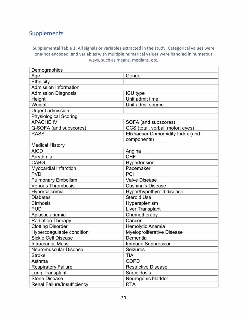
Supplemental Table 1: All signals or variables extracted in the study. Categorical values were

one-hot encoded, and variables with multiple numerical values were handled in numerous

ways, such as means, medians, etc. ..........................................................................................30

Supplemental Table 2: All signals or variables included in the best performing mixed features

model, totaling 53 features. Categorical values were one-hot encoded, and variables with

multiple numerical values were handled in numerous ways, such as means, medians, etc. ......33

Supplemental Table 3: Physiological ranges used to determine plausibility of high frequency

data. .........................................................................................................................................34

ix

List of Figures

Figure 1: Flow diagram of the study ICU stay selection process. ..................................................5

Figure 2: Complex features were extracted using the high-frequency data of each ICU stay, from

1-hour long chunks of time (labeled a through l) at the end of the ICU stay. These were then

aggregated into one feature space. .............................................................................................8

Figure 3: Complex features were extracted using the high-frequency data of each ICU stay, from

varying chunks of time (labeled a through e) at the end of the ICU stay. .....................................8

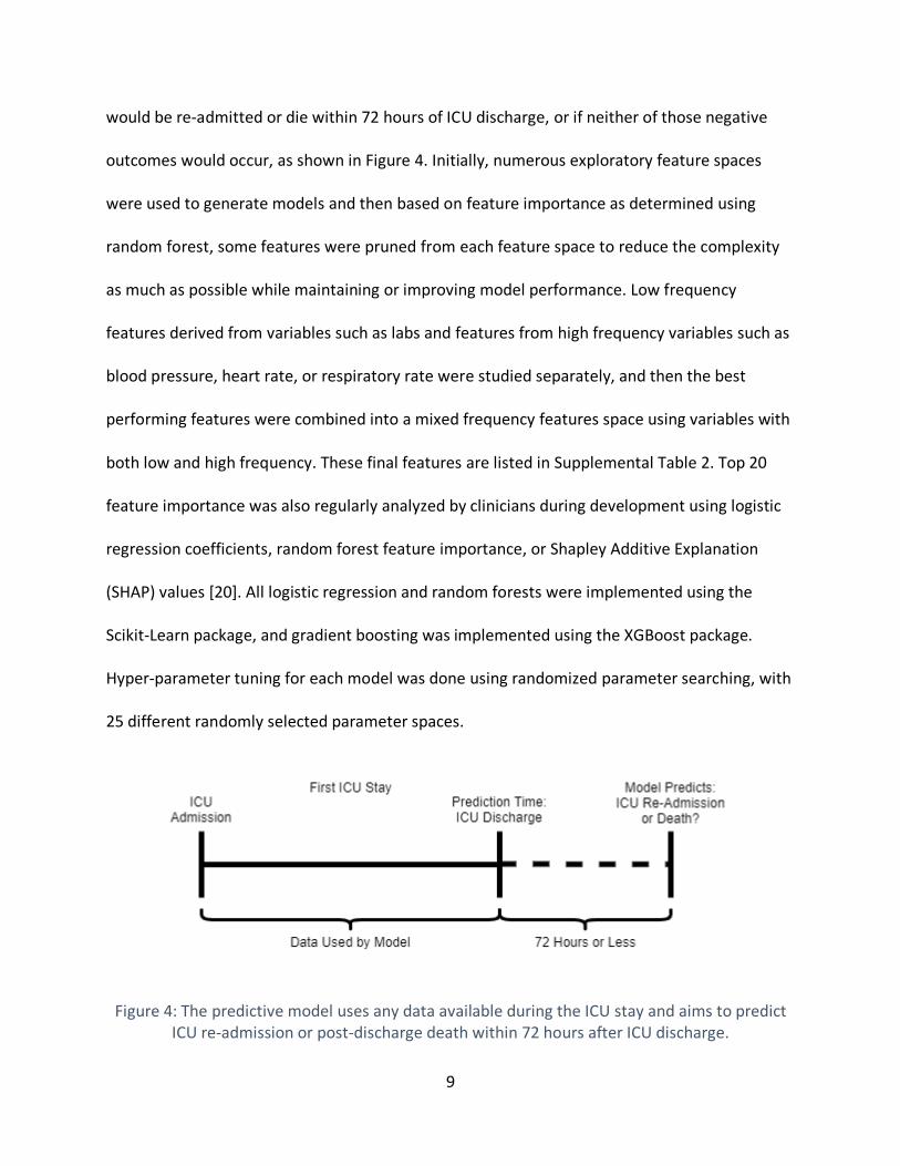
Figure 4: The predictive model uses any data available during the ICU stay and aims to predict

ICU re-admission or post-discharge death within 72 hours after ICU discharge. ..........................9

Figure 5: Performance of predictive models using random forest, with different feature spaces

and optimized feature importance thresholds for each feature space. High frequency feature

spaces were extracted as described in Figure 2 and Figure 3. ....................................................14

Figure 6: Effects on performance of feature importance thresholding. Each line represents the

performance of a predictive model created with different feature spaces, generally showing

there is a threshold in the middle that yields the highest performance. ....................................16

Figure 7: Feature importance as determined by the sklearn package’s random forest algorithm

of the top 20 features for the mixed feature space model. .......................................................17

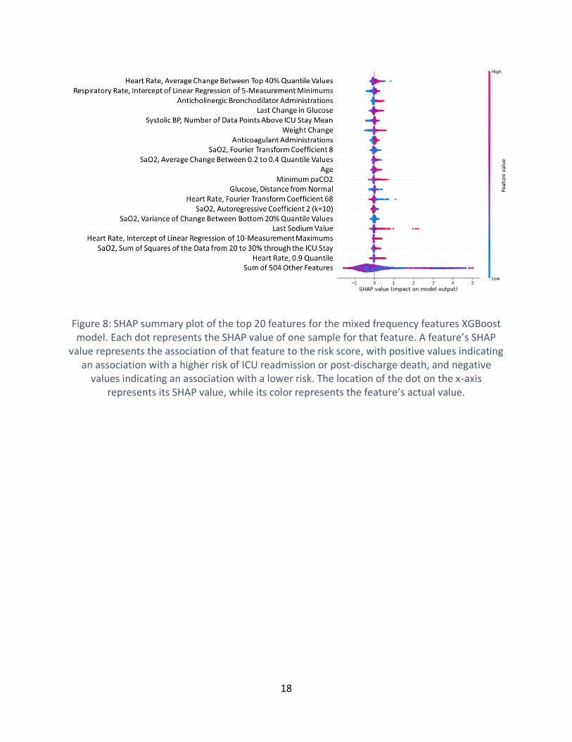
Figure 8: SHAP summary plot of the top 20 features for the mixed frequency features XGBoost

model. Each dot represents the SHAP value of one sample for that feature. A feature’s SHAP

value represents the association of that feature to the risk score, with positive values indicating

an association with a higher risk of ICU readmission or post-discharge death, and negative

x

values indicating an association with a lower risk. The location of the dot on the x-axis

represents its SHAP value, while its color represents the feature’s actual value. .......................18

1

Introduction

Consequences of ICU Readmissions

The deployment, utilization, and cost of critical care has been continually increasing for many

years. For example, the number of critical care beds has been continually increasing, relative to

population growth, and costs associated with critical care nearly doubled between 2000 and

2010, with the proportion of those costs to the gross domestic product increasing by 32.1% [1].

Critical illness is associated with increased medical resource utilization, even after survival and

hospital discharge [2]. As such, intensive care unit (ICU) readmissions contribute significantly to

resource utilization. ICU readmissions are also linked to negative patient outcomes. Patients

who are readmitted to ICUs tend to have higher risk for mortality, longer ICU stays, and overall

longer hospital stays, although these differences may be accounted for by severity of illness [3].

Difficulty of ICU Discharge Planning

The high resource and health costs of readmissions make prevention of ICU readmissions an

area of significant interest. Effective discharge planning is generally considered to be an

important aspect of preventing ICU readmissions [4], however, determining which patients are

ready for ICU discharge is difficult. For one, ICU readmission rates vary widely in different

settings, by country, hospital, or even individual unit, with rates as low as 0.89% (in an

American surgical ICU), or as high as 19.0% (in an American liver transplant ICU), likely because

there are a vast number of factors that can impact risk for ICU readmission [5, 6]. Unintended

delays in ICU discharge have been shown to reduce the likelihood of mortality in high-risk

patients, indicating that longer ICU stays in some instances can be beneficial [6]. However,

2

longer stays in the ICU have financial and logistical costs, meaning that holding patients too

long also has significant downsides. When the predictive performance of clinicians was directly

measured, performance was only modest, achieving area under the receiver operating curve

(AUROC) of about 0.70 on average [7].

Known Risk Factors for Readmission

Numerous studies have been conducted examining known risk factors or predictive features of

ICU readmissions or death, which point to many factors being predictive. Admission sources,

chronic health conditions, measures of severity, time of day at ICU discharge, age, sex,

socioeconomic status, and numerous other physiological factors have been indicated as

predictive in past studies [5, 3, 8, 9].

Existing Predictive Models

In recent years, machine learning approaches have also been applied to the problem,

attempting to leverage high resolution data to better identify patterns and predict ICU

readmissions in ways that were not previously possible. Despite numerous attempts using

various machine learning methods such as regression, tree-based methods, and even neural

networks, performance generally has been modest, approximately matching clinician

prediction. Performance of various studies ranged from about 0.6 to 0.8 AUROC, with various

populations and time frames of readmissions prediction [10, 11, 9, 12, 13, 14, 15]. None of the

found studies included complex features derived from high-frequency physiological time series

data, instead opting for simplistic features on high frequency data such as means, minimums, or

maximums, or variances [13, 16, 14, 12, 15].

3

Study Aims

We hypothesize that complex features constructed from high frequency time series data will

provide significant predictive power beyond that of traditional low-frequency variables. The aim

of this study is to create a model for predicting the probability of ICU readmissions or post-

discharge mortality within 72 hours of ICU discharge, by leveraging complex physiological time

series data and known clinical risk factors from a large multi-center database.

4

Methods

We used retrospective data to create a high-performing predictive model with the goal of

predicting ICU readmission or death within 72 hours after discharge from the ICU in surgical

patients. All code will be made publicly available on GitHub at

https://github.com/supatuffpinkpuff/icu-readmissions.

Database

Data were from the eICU Collaborative Research Database. The eICU Collaborative Research

Database [17] is a multi-center database containing highly granular data on 200,859 admissions

to ICUs from between 2014 and 2015 at 208 hospitals located in the United States.

Inclusion/Exclusion

ICU stays were included in the study if they were the index surgical ICU stays (that patient’s first

ICU stay with a surgical diagnosis), had no errors in data regarding their ICU stays and

readmission times, and had a length of stay of at least 2 hours. ICU stays were excluded if the

patient died in the ICU, was transferred to another ICU, was receiving comfort measures only,

or that were discharged with do not resuscitate orders and died after discharge. To ensure

signal quality, ICU stays were excluded if physiological time series data (PTS) for SaO2,

respiratory rate, heart rate, and blood pressure were not available for more than 50% of the

ICU stay and 50% of the last 24 hours of the ICU stay. These criteria are illustrated in Figure 1.

5

Figure 1: Flow diagram of the study ICU stay selection process.

High Frequency Signal Pre-Processing

High frequency variables provided in the eICU database are available at rates up to every 5

minutes, but with non-negligible amounts of erroneous or missing data. To enable the

calculation of complex features from these signals, some pre-processing was done. To begin,

6

physiologically implausible values were removed entirely from the data, based on clinician

adjudication. The criteria used are available in Supplemental Table 3. Such implausible values

represented less than 1% of data points for each signal’s data. On occasion, there would be

multiple data points with the same time stamp, in which case the data would be averaged so

that each time stamp had only one data point. Then, for oxygen saturation, respiratory rate,

and heart rate, any gaps shorter than 1 hour in the signal were linearly interpolated. For blood

pressure data, non-invasive and invasive data signals were overlaid, since most ICU patients

have one or the other, but rarely both. If both were present, then invasive data was presumed

to be correct, based on earlier analysis which showed that less than 0.1% of the invasive blood

pressure data was likely to be erroneous. Then any 2 hour or less gaps within the invasive/non-

invasive blood pressure data, or between invasive and non-invasive data were linearly

interpolated.

Feature Generation

Potentially useful signals and variables were identified with dataset exploration, clinician

guidance, and searching existing literature. Conventional, low frequency variables extracted

from data included demographics, medical history, labs, medications, medical scores,

comorbidities, dialysis, etc., which we refer to as the low frequency feature space. Common

statistics such as means, medians, and maximums, were used, but also some clinician-designed

features were created, such as the distance of the last measurement from a normal value, or

whether the data was trending towards a pre-defined normal value.

7

For especially frequent (up to every 5 minutes) respiratory rate, heart rate, blood pressure, or

oxygen saturation data, more complex feature transformations such as Fourier transform

coefficients or entropy were extracted using the tsfresh Python package. The tsfresh package

will automatically extract complex physiological features when given cleaned time series data.

These high frequency features were generated in several ways, with different methods of

temporally segmenting the physiological signal data. In the first method the last 12 hours of

data before discharge by splitting it into 1-hour long intervals and extracting features from

those, as seen in Figure 2, which could yield predictive information based on how those

features evolve from hour to hour. This was done for each high-frequency signal individually,

including oxygen saturation, respiratory rate, heart rate, and systolic/diastolic/mean blood

pressure, yielding six different high frequency feature spaces. The second method was to

extract features from all signals during longer, variable duration intervals of time at the end of

the ICU stay, which could yield information from the entire time period analyzed, shown in

Figure 3. This yielded an additional six high frequency feature spaces from each different

interval length.

For all features, missing values were imputed using several different approaches. Mean

imputation and median imputation were explored, with median imputation being used in the

final model. A full list of all variables (low and high frequency) explored can be found in

Supplemental Table 1.

8

Figure 2: Complex features were extracted using the high-frequency data of each ICU stay, from 1-hour long chunks of time (labeled a through l) at the end of the ICU stay. These were then

aggregated into one feature space.

Figure 3: Complex features were extracted using the high-frequency data of each ICU stay, from varying chunks of time (labeled a through e) at the end of the ICU stay.

Modeling Approaches

Three machine learning algorithms were used to construct the predictive model, namely logistic

regression, random forest [18], and gradient boosting [19], chosen for their ease of use and

high predictive performance in other complex problems. These were used to construct models

that could, at time of discharge, predict a composite outcome, of whether a surgical ICU patient

9

would be re-admitted or die within 72 hours of ICU discharge, or if neither of those negative

outcomes would occur, as shown in Figure 4. Initially, numerous exploratory feature spaces

were used to generate models and then based on feature importance as determined using

random forest, some features were pruned from each feature space to reduce the complexity

as much as possible while maintaining or improving model performance. Low frequency

features derived from variables such as labs and features from high frequency variables such as

blood pressure, heart rate, or respiratory rate were studied separately, and then the best

performing features were combined into a mixed frequency features space using variables with

both low and high frequency. These final features are listed in Supplemental Table 2. Top 20

feature importance was also regularly analyzed by clinicians during development using logistic

regression coefficients, random forest feature importance, or Shapley Additive Explanation

(SHAP) values [20]. All logistic regression and random forests were implemented using the

Scikit-Learn package, and gradient boosting was implemented using the XGBoost package.

Hyper-parameter tuning for each model was done using randomized parameter searching, with

25 different randomly selected parameter spaces.

Figure 4: The predictive model uses any data available during the ICU stay and aims to predict ICU re-admission or post-discharge death within 72 hours after ICU discharge.

10

Evaluation of Model Performance

The model performance was primarily evaluated using the area under the receiver operating

curve (AUROC), a general metric of predictive performance, as well as a 95% confidence

interval of that performance. First a training set was created using 80% of the data, leaving the

remaining 20% as a held-out test set. Models were developed and evaluated on the training set

using nested cross validation, with 3 inner folds and 5 outer folds. The best performing

hyperparameters and features obtained from the cross validation were then used to make

predictions on the test set and obtain AUROC. Different feature spaces were compared to

evaluate the effectiveness of different groups of variables.

11

Results

Study selection resulted in 24,177 ICU stays total, with 23,367 labeled as no readmission and

survived, and 810 with a readmission or death within 72 hours of ICU discharge, representing a

3.35% readmission or post-discharge mortality rate, as seen in Figure 1. Various characteristics

of ICU stays used in the model can be found in Table 1. Characteristics of the hospitals these

ICU stays originated from can be found in Table 2.

Table 1: Characteristics of ICU Stays, split by label and with p-values of comparisons between the cases and controls using Mann-Whitney for numeric variables or chi-squared testing for

categorical variables.

No Readmit/Death Readmit/Death Total p-Value

Patient Characteristics Gender 0.842

Male 13298 (56.91%) 469 (57.9%) 13767 (56.94%)

Female 10069 (43.09%) 341 (42.1%) 10410 (43.06%)

Median Age [IQR] (Years) 66.0 [56.0-75.0] 69.0 [59.0-77.0] 66.0 [56.0-75.0] < 0.001

Ethnicity 0.990 Caucasian 18461 (80.29%) 647 (80.37%) 19108 (80.29%)

African American 1864 (8.11%) 59 (7.33%) 1923 (8.08%)

Other/Unknown 1149 (5.0%) 34 (4.22%) 1183 (4.97%)

Hispanic 924 (4.02%) 40 (4.97%) 964 (4.05%)

Asian 458 (1.99%) 20 (2.48%) 478 (2.01%)

Native American 138 (0.6%) 5 (0.62%) 143 (0.6%)

Median First 24 Hour APACHE IV Score [IQR]

47.0 [36.0-61.0] 55.0 [42.75-73.0] 48.0 [36.0-62.0] < 0.001

Admission Source 0.999

Operating Room 16276 (69.72%) 567 (70.0%) 16843 (69.73%)

Recovery Room/PACU 5929 (25.40%) 197 (24.32%) 6126 (25.36%)

Floor 421 (1.8%) 18 (2.22%) 439 (1.82%)

Emergency Department 349 (1.49%) 14 (1.73%) 363 (1.5%)

Other 371 (1.54%) 14 (1.73%) 385 (1.59%)

Primary Diagnostic Groupings (Per eICU Database) 0.484 Cardiovascular 11141 (47.68%) 324 (40.0%) 11465 (47.42%)

Gastrointestinal 3678 (15.74%) 205 (25.31%) 3883 (16.06%)

Neurologic 3663 (15.68%) 108 (13.33%) 3771 (15.6%)

Respiratory 1780 (7.62%) 72 (8.89%) 1852 (7.66%)

Genitourinary 969 (4.15%) 26 (3.21%) 995 (4.12%)

12

Musculoskeletal/Skin 967 (4.14%) 32 (3.95%) 999 (4.13%)

Trauma 853 (3.65%) 32 (3.95%) 885 (3.66%)

Transplant 181 (0.77%) 10 (1.23%) 191 (0.79%)

Metabolic/Endocrine 126 (0.54%) 1 (0.12%) 127 (0.53%)

Hematology 9 (0.04%) 0 (0%) 9 (0.04%)

Outcomes

Median ICU LOS [IQR] (Hours) 32.98 [22.69-65.31] 43.25 [24.1-87.35] 33.48 [22.75-65.7] < 0.001

Hospital Mortality < 0.001 Alive 23091 (99.38%) 692 (86.39%) 23783 (98.95%)

Expired 144 (0.62%) 109 (13.61%) 253 (1.05%)

Table 2: Characteristics of the 185 hospitals from which ICU stays in this study were drawn.

Hospital Trait Number of Hospitals (Proportion)

Size

<100 Beds 35 (23.2%)

100 – 249 Beds 59 (39.1%)

250 – 499 Beds 34 (22.5%)

>= 500 Beds 23 (15.2%)

Region

Midwest 61 (37.7%)

South 50 (30.9%)

West 39 (24.1%)

Northeast 12 (7.4%)

Teaching Status

Non-Teaching Hospital 166 (89.7%)

Teaching Hospital 19 (10.3%)

13

Traditional vs. High Frequency Physiological Signals

The predictive performance of many different feature spaces with different feature importance

thresholds was compared, using AUROCs from both the outer loop of the nested cross

validation (i.e., training), and a test set never seen by the model during training. In the training

results the mixed feature space that uses both low and high frequency variables (AUROC =

0.680, 95% CI = [0.647, 0.713]) performed similarly to the low frequency variable feature space

(mean AUROC = 0.671, 95% CI = [0.636, 0.706]) alone. The various feature spaces constructed

from high frequency variables did not perform as well, which can be seen in Figure 5. With

regards to the test set, the mixed feature space performed best (AUROC = 0.656) by several

hundredths, as opposed to the low frequency variables alone (AUROC = 0.607) or the best high-

frequency feature space (AUROC = 0.647).

14

Figure 5: Performance of predictive models using random forest, with different feature spaces and optimized feature importance thresholds for each feature space. High frequency feature

spaces were extracted as described in Figure 2 and Figure 3.

Comparison of Machine Learning Algorithms

Three machine learning algorithms were used for modeling in this study: logistic regression,

random forest, and XGBoost. Random forest and XGboost performed essentially equivalently,

with random forest performing slightly better, but within one standard deviation of XGBoost’s

performance, as seen when using a mixed frequency feature space in Table 3. Logistic

regression performance was particularly poor, even achieving AUROCs below 0.5.

15

Table 3: Predictive performance of different algorithms on the full mixed frequency feature space.

Algorithm Mean Outer Loop AUROC

Outer Loop AUROC Standard Deviation

Test Set AUROC

Logistic Regression 0.480 0.012 0.500

Random Forest 0.676 0.025 0.649

XGBoost 0.668 0.018 0.646

Effects of Model Pruning

To reduce the size of the feature space used in the models and therefore increase calculation

speed, the feature importance metric provided by the Scikit-Learn package’s random forest

model was used. In each feature space, low importance features were iteratively pruned from

the model using higher and higher importance thresholds. Across many exploratory feature

spaces, the predictive performance would generally decrease slightly with low importance

thresholds, match or even slightly outperform the full feature space at medium thresholds, and

then finally decrease again at high thresholds, as seen in Figure 6. Other features space,

including the highest-performing mixed frequency features space, simply saw continual

performance improvements as more features were cut, down to 10% of features being kept.

16

Figure 6: Effects on performance of feature importance thresholding. Each line represents the performance of a predictive model created with different feature spaces, generally showing

there is a threshold in the middle that yields the highest performance.

Feature Importance Analysis

The most important features of models were analyzed using random forest feature importance

values to identify the top 20 most predictive features. When using the highest performing

mixed feature space, the top 20 features included both low and high frequency variables, as

seen in Figure 7. The top features derived from high-frequency variables included measures of

non-linearity, anomaly detection, linear regression intercepts, and Fourier Transform attributes.

Most of these came from heart rate and respiratory rate data, although SaO2 did yield one

highly important feature. Blood pressure features did not appear in the top 20 most important

features at all. Important features derived from low-frequency variables include several

17

measures of sodium level in the blood, change between the last two glucose measurements,

APACHE IV score, and ICU length of stay.

Figure 7: Feature importance as determined by the sklearn package’s random forest algorithm of the top 20 features for the mixed feature space model.

Top features were also analyzed using Shapley Additive Explanations (SHAP) values, calculated

using the shap package. This enables some interpretability analysis in addition to analyzing

which features were most important. This analysis yielded a very different top 20 features, still

including labs like glucose and sodium, as well as numerous high frequency features based on

heart rate, respiratory rate, and oxygen saturation. Of note, age, paCO2, weight change, and

administrations of anticholinergic bronchodilators and anticoagulants were deemed highly

important by SHAP values in the XGBoost model, none of which appeared in the random forest

analysis. More detailed information regarding the relationships between the top features and

model output can be seen in Figure 8.

18

Figure 8: SHAP summary plot of the top 20 features for the mixed frequency features XGBoost model. Each dot represents the SHAP value of one sample for that feature. A feature’s SHAP

value represents the association of that feature to the risk score, with positive values indicating an association with a higher risk of ICU readmission or post-discharge death, and negative

values indicating an association with a lower risk. The location of the dot on the x-axis represents its SHAP value, while its color represents the feature’s actual value.

19

Discussion

Main Findings

Thus far, the predictive performance of the models constructed in this study is comparable to

clinician prediction and existing models, excluding one unusually high-performing model from a

single hospital in Brazil, as seen in Table 4. We hypothesized that leveraging a large dataset,

high frequency variables, and complex features would achieve higher performance. The

inability to confirm this could be due in part to the highly heterogeneous nature of this dataset,

or perhaps because we studied surgical ICU patients specifically, which differs from previous

approaches. The usage of features from high frequency variables does marginally increase

performance in comparison to using only traditional low frequency variables, but only on the

test set, and not during cross-validation. With the features currently being used, this seems to

indicate the features derived from high frequency signals are capturing some information

useful for predicting ICU readmissions and post-discharge mortality, but it is likely not different

information from that obtained via traditional low-frequency variables.

Table 4: Analysis of recent studies on high performing prediction methods for ICU readmissions.

Prediction Method Year Sample Size

Patient Description

Best AUROC

Hospitals in Study

Re-admission Rate

Logistic Regression, Random Forest, XGBoost [this study]

2021 24,177 Index Surgical ICU Stay

0.680 185 3.35%

Clinician Prediction [7]

2020 2,833 Medical ICU Patients

0.70 1 4%

Logistic Regression [13]

2012 704,963 Adult ICU Patients

0.71 219 2.5%

20

Fuzzy Models [16] 2012 1,028 Adult ICU Patients

0.72 1 13%

XGBoost [11] 2018 24,885 Adult ICU Patients

0.76 1 11%

Bayesian algorithms, decision trees, rule-based, ensemble methods [21]

2020 9,926 Adult ICU Patients

0.91 1 6.6%

Analysis of our Models

High Frequency Time Series Features

This study sought to explore the usefulness of complex features derived from high frequency

physiological data and did find that on the test set, including some of these features improved

the performance of our model when compared to predictive models built using just low

frequency variables only, as seen in Figure 5. However, performance obtained using cross

validation did not increase beyond a 95% confidence interval, indicating this difference is not

statistically significant. Further study to identify why the test set performance differs so much is

warranted. Numerous complex features did appear to be the most predictive when analyzed

using random forest feature importance values, as indicated in Figure 7, and when using SHAP

values, as seen in Figure 8. This could mean that these complex features do have some use in

predicting ICU readmissions or post discharge mortality, but that it is likely not capturing much

novel information compared to the low-frequency features.

21

Large and Heterogeneous Dataset

Our study uses data from the Philips eICU database, which is large and includes many hospitals

across the United States. We extracted 24,177 ICU stays from 185 hospitals across the United

States dataset for training, testing, and validating our model. This is more ICU stays than the

datasets used by most previous models and is likely to have far more heterogeneity than the

data used in previous studies, many of which examined data from only a single hospital. This

heterogeneity likely makes our findings more broadly applicable, especially in the United States

where all the data was obtained.

Feature Interpretability and Analysis

The top feature analysis conducted using random forest (Figure 7) is not able to examine the

relationships between features and model output but does still indicate which features were

considered most important to prediction by the model. The most important features seem

plausibly correlated with readmission or mortality. The top features derived from high-

frequency variables included measures of non-linearity, anomaly detection, linear regression

intercepts, and Fourier Transform attributes, which are likely indicators of trends and stability

in those physiological signals. Blood pressure features did not appear in the top 20 most

important features at all, indicating perhaps that blood pressure data are less useful or that

relevant features for blood pressure were not utilized in this study. Other top features include

several measures of sodium level in the blood and recent changes in glucose, which are likely

associated with illnesses that increase medical risk such as kidney problems, diabetes, or

trauma. Unsurprisingly, APACHE IV score and ICU length of stay also were top features based on

the random forest analysis, likely as indicators of overall illness severity.

22

Using SHAP value analysis, it is possible to examine the relationships between specific features

and model output, which can be seen in Figure 8. Many of the relationships among the top 20

features seem physiologically plausible. For example, high weight gain during the ICU stay was

associated with higher risk of readmission or mortality, likely a proxy for circulatory volume

overload or over-resuscitation seen in critically ill patients with conditions like decompensated

heart failure or septic shock. Likewise, administrations of anticholinergic bronchodilators and

anticoagulants were associated with higher risks, possibly because the underlying reason for

which those drugs were administered (difficulty breathing for bronchodilators, or

cardiovascular problems for anticoagulants). The numerous complex features on heart rate,

blood pressure, respiratory rate, or oxygen saturation data could have many clinical

interpretations. Some of these capture directional trends in the data, or variability, both of

which might indicate a lack of physiological stability. Other relationships between features and

model output were less clear-cut and require further analysis. SHAP values can also be used to

examine interactions between features, although no feature interactions of interest were found

thus far.

Limitations of our Models

Data Quality

One significant limitation of our data was the amount of missing data. Since this is a publicly

available database compiled in the past, we had no control over the actual collection process of

the data, and little insight into exactly why certain data were missing or erroneous. We were

able to guess to some degree why data might be missing and accordingly made decisions about

inclusion and pre-processing, but such hypotheses cannot be verified. Certain ICU stays in our

23

dataset were excluded due to data quality issues, such as missing certain important

physiological time series features. The eICU database is also built from data collected during

routine care, and as such is missing potentially valuable data. For example, time series data is at

best measured every 5 minutes, while data sampled at a higher frequency, or waveform data,

might contain more predictive information. There is also little data about social determinants of

health or provider/hospital traits.

Correlational Relationships Between Variables and Labels

Although feature ranking and analyses such as Shapley summary plots can help to show some

of the relationships between features and the outcome label, it is difficult to exactly interpret

how complex machine learning models are making predictions. It is not currently feasible to

display information about all of the complexity of model outputs, such as interactions and

feature effects on output simultaneously. In addition, the constructed predictive models are

largely based on statistical correlation: they are not capable of identifying causal relationships,

meaning that model features may only be proxies for actual causal variables.

United States Hospitals

All the hospitals in the eICU database are in the United States. This means all the data used to

train and test our models are from United States hospitals, potentially limiting generalizability

of our results in other countries. This is especially likely given that ICU readmissions are

impacted by non-physiological factors, which may vary heavily between countries with different

medical practices and health system operational paradigms.

24

Conclusion

Our newly developed models do not currently outperform previously constructed models in the

literature nor clinician prediction. The use of complex features derived from high frequency

physiological time series does slightly improve performance on the test set, but not beyond a

95% confidence interval on the outer loop results. Features derived from high frequency

physiological time series data do not currently appear to be useful in predicting ICU

readmissions or post-discharge mortality, although clearly further investigation is warranted.

Expansion Possibilities

There are many ways we could build upon the current predictive model. While thus far

simplistic methods for imputation such as median or mean imputation were used, many

variables would likely benefit from multiple imputation, based on patient characteristics such

gender, age, or weight. Additional predictive features could also be added to improve

performance, either based on entirely different variables, or perhaps using other complex

features derived from high frequency data. It is possible that other types of features besides

those extracted by the tsfresh package could be useful, or perhaps that other frameworks to

extract features would yield better performance, such as different interval lengths or

combinations of interval features than used in this study (Figure 2, Figure 3). Those additional

features might require entirely different datasets, such as more frequent time series data,

socioeconomic factors, genetic analysis, or more hospital characteristics. Further analysis of

feature relationships and interactions could also be done, especially with clinician and

mathematician collaboration to fully understand both the mathematical and physiological

meaning of complex time series features. Finally, there was significant class imbalance in the

25

dataset, which could potentially be addressed with over or under sampling, or methods such as

Synthetic Minority Over-sampling Technique (SMOTE) [22]. If these methods improve model

performance, it would then be worthwhile to explore additional model metrics such as model

calibration, externally validate these results to increase confidence that the model is universally

applicable, and after that potentially conduct prospective studies of model performance.

26

References

[1] N. A. Halpern, D. A. Goldman, K. S. Tan and S. M. Pastores, "Trends in critical care beds

and use among population groups and Medicare and Medicaid beneficiaries in the United

States: 2000–2010," Crit Care Med, vol. 44, no. 8, pp. 1490-1499, 2016.

[2] E. L. Hirshberg, E. L. Wilson, V. Stanfield, K. G. Kuttler, S. Majercik, S. J. Beesley, J. Orme, R.

O. Hopkins and S. M. Brown, "Impact of Critical Illness on Resource Utilization: A

Comparison of Use in the Year Before and After ICU Admission," Crit Care Med, vol. 47,

no. 11, pp. 1497-1503, 2019.

[3] A. A. Kramer, T. L. Higgins and J. E. Zimmerman, "The Association Between ICU

Readmission Rate and Patient Outcomes," Crit Care Med, vol. 41, no. 1, pp. 24-33, 2013.

[4] U. R. Ofoma, Y. Dong, O. Gajic and B. W. Pickering, "A qualitative exploration of the

discharge process and factors predisposing to readmissions to the intensive care unit,"

BMC Health Services Research, vol. 18, no. 6, 2018.

[5] J. Renton, D. V. Pilcher, J. D. Santamaria, P. Stow, M. Bailey, G. Hart and G. Duke, "Factors

associated with increased risk of readmission to intensive care in Australia," Intensive Care

Med, p. 1800–1808, 2011.

27

[6] G. M. Forster, S. Bihari, R. Tiruvoipati, M. Bailey and D. Pilcher, "The Association between

Discharge Delay from Intensive Care and Patient Outcomes," Am J Respir Crit Care Med,

vol. 202, no. 10, pp. 1399-1406, 2020.

[7] J. C. Rojas, P. G. Lyons, T. Jiang, M. Kilaru, L. McCauley, J. Picart, K. A. Carey, D. P. Edelson,

V. M. Arora and M. M. Churpek, "Accuracy of Clinicians’ Ability to Predict the Need for

Intensive Care Unit Readmission," Ann Am Thorac Soc, vol. 17, no. 7, pp. 847-853, 2020.

[8] A. Garland, K. Olafson, C. D. Ramsey, M. Yogendran and R. Fransoo, "Epidemiology of

critically ill patients in intensive care units: a population-based observational study,"

Critical Care, vol. 17, no. 5, p. R212, 2013.

[9] N. Markazi-Moghaddam, M. Fathi and A. Ramezankhani, "Risk prediction models for

intensive care unit readmission: A systematic review of methodology and applicability,"

Australian Critical Care, vol. 33, pp. 367-374, 2020.

[10] S. Barbieri, J. Kemp, O. Perez-Concha, S. Kotwal, M. Gallagher, A. Ritchie and L. Jorm,

"Benchmarking Deep Learning Architectures for Predicting Readmission to the ICU and

Describing Patients-at-Risk," Scientific Reports, 2020.

[11] J. C. Rojas, K. A. Carey, D. P. Edelson, L. R. Venable, M. D. Howell and M. M. Churpek,

"Predicting Intensive Care Unit Readmission with Machine Learning Using Electronic

Health Record Data," Annals ATS, vol. 15, no. 7, pp. 846-853, 2018.

28

[12] R. G. Rosa, C. Roehrig, R. P. d. Oliveira, J. G. Maccari, A. C. P. Antonio, P. d. S. Castro, F. L.

D. Neto, P. d. C. Balzano and C. Teixeira, "Comparison of Unplanned Intensive Care Unit

Readmission Scores: A Prospective Cohort Study," PLoS ONE, vol. 10, no. 11, 2015.

[13] O. Badawi and M. J. Breslow, "Readmissions and Death after ICU Discharge: Development

and Validation of Two Predictive Models," PLoS ONE, vol. 7, no. 11, 2012.

[14] Y.-W. Lin, Y. Zhou, F. Faghri, M. J. Shaw and R. H. Campbell, "Analysis and prediction of

unplanned intensive care unit readmission using recurrent neural networks with long

short-term memory," PLoS ONE, vol. 14, no. 7, 2019.

[15] M. Hammer, S. D. Grabitz, B. Teja, K. Wongtangman, M. Serrano, S. Neves, S. Siddiqui, X.

Xu and M. Eikermann, "A Tool to Predict Readmission to the Intensive Care Unit in Surgical

Critical Care Patients—The RISC Score," Journal of Intensive Care Medicine, 2020.

[16] A. S. Fialho, F. Cismondi, S. M. Vieira, S. R. Reti, J. M. Sousa and S. N. Finkelstein, "Data

mining using clinical physiology at discharge to predict ICU readmissions," Expert Syst

Appl, vol. 39, pp. 13158-13165, 2012.

[17] T. J. Pollard, A. E. Johnson, J. D. Raffa, L. A. Celi, R. G. Mark and O. Badawi, "The eICU

Collaborative Research Database, a freely available multi-center database for critical care

research.," Scientific Data, 2018.

[18] L. Breiman, "Random Forests," Machine Learning, vol. 45, pp. 5-32, 2001.

[19] T. Chen and C. Guestrin, "XBGoost: A Scalable Tree Boosting System," arXiv, 2016.

29

[20] S. M. Lundberg, B. Nair, M. S. Vavilala, M. Horibe, M. J. Eisses, T. Adams, D. E. Liston, D. K.-

W. Low, S.-F. Newman, J. Kim and S.-I. Lee, "Explainable machine-learning predictions for

the prevention of hypoxaemia during surgery," Nat Biomed Eng, vol. 2, no. 10, pp. 749-

760, 2018.

[21] M. Loreto, T. Lisboa and V. P. Moreira, "Early prediction of ICU readmissions using

classification algorithms," Comput Biol Med, vol. 118, p. 103636, 2020.

[22] N. V. Chawla, K. W. Bowyer, L. O. Hall and W. P. Kegelmeyer, "SMOTE: Synthetic Minority

Over-sampling Technique," J Artif Intell Res, vol. 16, pp. 321-357, 2002.

30

Supplements

Supplemental Table 1: All signals or variables extracted in the study. Categorical values were one-hot encoded, and variables with multiple numerical values were handled in numerous

ways, such as means, medians, etc.

Demographics

Age Gender

Ethnicity

Admission Information

Admission Diagnosis ICU type

Height Unit admit time

Weight Unit admit source

Urgent admission

Physiological Scoring

APACHE IV SOFA (and subscores)

Q-SOFA (and subscores) GCS (total, verbal, motor, eyes)

RASS Elixhauser Comorbidity Index (and components)

Medical History

AICD Angina

Arrythmia CHF

CABG Hypertension

Myocardial Infarction Pacemaker

PVD PCI

Pulmonary Embolism Valve Disease

Venous Thrombosis Cushing’s Disease

Hypercalcemia Hyper/hypothyroid disease

Diabetes Steroid Use

Cirrhosis Hypersplenism

PUD Liver Transplant

Aplastic anemia Chemotherapy

Radiation Therapy Cancer

Clotting Disorder Hemolytic Anemia

Hypercoagulable condition Myeloproliferative Disease

Sickle Cell Disease Dementia

Intracranial Mass Immune Suppression

Neuromuscular Disease Seizures

Stroke TIA

Asthma COPD

Respiratory Failure Restrictive Disease

Lung Transplant Sarcoidosis

Stone Disease Neurogenic bladder

Renal Failure/Insufficiency RTA

31

Renal Transplant Rheumatic Disease

Labs

Albumin Alkaline Phosphate

ALT (SGPT) Anion gap

AST (SGOT) Glucose

BUN Calcium

Chloride Creatinine

Hct Hgb

Lactate Lymphs

Magnesium MCH

MCHC MCV

Monos MPV

O2 Saturation paCO2

paO2 pH

Phosphate Platelets

Polys Potassium

PT PT – INR

RBC RDW

Sodium Total bilirubin

Total protein WBC

Bicarbonate

Medications

Acetaminophen Adrenergic Bronchodilators

Aminoglycosides Anticholinergic Bronchodilators

Anticholinergics Anticoagulants

Antidiarrheals Antiemetics

Antihistamines Barbiturates

Benzodiazepines Beta Blockers

Calcium Channel Blockers Carbapenems

Cephalosporins Class V Antiarrhythmics

Colloid fluids Crystalloid fluids

Diuretics General Anesthetics

Glucocorticoids Glucose Elevating Drugs

Glycopeptides H2 Receptor Blockers

Haloperidol Insulin

Laxatives Lincomycins

Macrolides MAOI Antidepressants

Methylxanthines Other antidepressants

Potassium Channel Blockers Precedex

Proton Pump Inhibitor Quinolones

SNRI Antidepressants Sodium Channel Blockers

Somatostatin SSRI Antidepressants

Sulfonamides Tetracyclic Antidepressants

Tetracyclines Thrombolytics

Tricyclic Antidepressants Vasodilators

32

Vasopressors

Physiological Measurements

Temperature Blood pressure

SaO2 Respiratory Rate

Heart rate Urine output

Treatments

Dialysis Mechanical Ventilation

Blood product transfusions (RBC, plasma, platelets, other)

Surgery

Miscellaneous

Infection Sepsis

Acute kidney injury Current LOS/Time of Day

Signals used with tsfresh package. Full list of features at: https://tsfresh.readthedocs.io/en/latest/text/list_of_features.html

SaO2 Blood pressure (systolic, diastolic, mean)

Respiratory Rate Heart Rate

33

Supplemental Table 2: All signals or variables included in the best performing mixed features model, totaling 53 features. Categorical values were one-hot encoded, and variables with multiple numerical values were handled in numerous ways, such as means, medians, etc.

Admission Information

Unit admit source Unit admit time

Weight

Urgent admission

Physiological Scoring

APACHE IV

Labs

ALT (SGPT) Anion gap

Creatinine Glucose

Chloride MCHC

O2 Saturation paCO2

Phosphate pH

Potassium Sodium

WBC

Miscellaneous

Current LOS Time of Day

Signals used with tsfresh package. Full list of features at: https://tsfresh.readthedocs.io/en/latest/text/list_of_features.html SaO2 Blood pressure (systolic, diastolic, mean)

Respiratory Rate Heart Rate

34

Supplemental Table 3: Physiological ranges used to determine plausibility of high frequency data.

Variable Lower Bound Upper Bound

SaO2 50% 100%

Heart Rate 20 bpm 220 bpm

Respiratory Rate 5 bpm 50 bpm

Systolic Blood Pressure 20 mmHg 300 mmHg

Diastolic Blood Pressure 5 mmHg 225 mmHg

Mean Blood Pressure 10 mmHg 250 mmHg

Pulse Pressure 5 mmHg 200 mmHg

Systolic – Mean Blood Pressure 3 mmHg N/A