Identifying RegressionOutliers and Mixtur esGraphically

R. DennisCook�

FrankCritchley�

February13,2000

Abstract

Regressionsin practicecanincludeoutliersandotherunknown subpop-ulation structure.For example,mixturesof regressionsoccurif thereis anomittedcategoricalpredictorlikegenderor locationanddifferentregressionsoccurwithin eachcategory. Thetheoryof regressiongraphicsbasedon cen-tral subspacescanbeusedto constructgraphicalsolutionsto long-standingproblemsof this type. It is arguedthat in practicethe centralsubspaceau-tomaticallyexpandsto incorporateoutliersandregressionmixtures. Thus,methodsof estimatingthecentralsubspacecanbeusedto identify thesephe-nomena,withoutspecifyinga model. Examplesillustratingthepower of thetheoryarepresented.

KeyWords: Central subspaces,Lurking variables,Regressiongraphics,Slicedinverseregression,Slicedaveragevariance estimation.

1 Intr oduction

Dimensionreductionis a leitmotif of statistics.For instance,startingwith asample�������������� from a univariatenormalpopulationwith mean � andvariance1, weknow that thesamplemean � is sufficient for � . This meansthat we canreplacetheoriginal � -dimensionalsamplewith theone-dimensionalmean � without lossof informationon � .�

Departmentof Applied Statistics,1994Buford Ave., University of Minnesota,St. Paul, MN55108.Thiswork wassupportedin partby NationalScienceFoundationgrantDMS-9703777.�

Schoolof MathematicsandStatistics,Universityof Birmingham,Edgbaston,BirminghamB152TT, UK. This work wassupportedin part by EPSRCgrant GR/K08246and the linked VisitingFellowshipGR/K71103.Theauthorsaregratefulto theassociateeditor for commentsthat resultedin notableimprovementsto thisarticle.

1

In thesamespirit, dimensionreductionwithout lossof informationis a domi-nantthemeof regressiongraphics.Thegoalof a regressionstudyis to infer abouttheconditionaldistribution of theresponse� giventhe ����� vectorof predictors�

. A centralgoalof regressiongraphicsis to reducethedimensionof�

withoutlossof informationon the conditionaldistribution of ��� � andwithout requiringa model.We call this sufficientdimensionreduction, borrowing terminologyfromclassicalstatistics.Sufficientdimensionreductionleadsnaturallyto sufficientsum-maryplotswhich containall of the informationon theregressionthat is availablefrom thesample(Cook1998b).Suchsummaryplotsmaybeparticularlyusefulforguiding the choiceof a first modelat thebeginning of analysis,andfor studyingresidualsafteramodelhasbeendeveloped.As reviewedin Section2.2,thecentralsubspace(Cook 1994b,1996,1998b)is a meta-parameterthat serves asa focalpoint for constructingestimatesof sufficient summaryplotsin practice.

We arguein this article that regressiongraphicscanbe usefulfor identifyingmixturesof regressionsin a largely nonparametriccontext. Sinceoutlierscanberegardedascasesarisingfrom laws thataredistinct from thoseunderstudy, theyareincludedunderthemixtureumbrella.Ourargumentis basedon theconclusionthat in practicethecentralsubspacewill usuallyexpandto incorporateregressionstructureinducedby mixtures. This implies that summaryplots arisingfrom es-timatesof the centralsubspacecanbe expectedto show mixturesalongwith themainregressionstructure.

Mixtures of regressionsoccurwhenthereis an omittedcategorical predictor,like gender, speciesor location,anddifferentregressionsoccurin eachcategory.It haslong beenrecognizedthat a lurking variable,a variablethat hasan impor-tanteffect but is not presentamongthepredictorsunderconsideration(Box 1966,Joiner1981,Moore1997),cancomplicateregressionanalyses.Ourresultsindicatethatregressiongraphicshastheability to suggestthepresenceof lurking variables,althoughit cannotidentify the variableitself. Nevertheless,whererelevant dataareavailable, it may be possibleto go on and identify suchvariables,as in theAustralianSportexampleof Section7.1.

By definition, an outlier mustoutlie something. Perhapsthe main approachto identifying outliers in regressionis basedon finding casesthat outlie a para-metricmodelfor theconditionaldistribution of ��� � . While it is well-known thatthe presenceof an outlier can indicatea deficiency in the modelor an abnormalcase,model-basedoutlier methodsstill seemto dominatetheliterature.A notableexceptionto this is in regressionswith a singlepredictorwhereoutliersareoftenidentifiedeasilyin a scatterplot of � versus� without specifyinga model. Thenotion that “you will know it whenyou seeit” seemsto characterizethemethodsinceit maybeeasyto spotthemainpatternin aplot while simultaneouslyrecog-nizing grossdeviationsfrom thatpattern,avoiding theneedto pre-specifya para-

2

metricmodel. As shown in this article,regressiongraphicsextendsvisualoutlierandsubpopulationrecognitionto regressionswith many predictors.

In the next sectionwe describethe populationcontext for our investigation.This includesadescriptionof theregressionmixtureandbackgroundonthecentralsubspace.Wediscussthemainpopulationresultsfromourinquiry in Section3. Weturnto estimationin Section4. Therewebriefly review methodsthatcanbeusedtoestimatethecentralsubspaceandconstructsummaryplots. In Sections5 and6 weinvestigatepropertiesof two methods– SAVE andSIR – in thecontext of thispaper.We describethreeapplicationsin Section7 that illustratethepotentialadvantagesof our approach.Concludingcommentsaregiven in Section8. Justificationsformostresultscanbefoundin theAppendix.

Thenotation� � meansthattherandomvectors� and � areindependent.Similarly, � ����� meansthat � and � areindependentgivenany valuefor therandomvector � . Subspaceswill usuallybe denotedby , and "!$#&% meansthesubspaceof ' (*) spannedby thecolumnsof the+-,/. matrix # . Thetrivial subspacecomprisingjust the origin is thus denotedby "!$01% . The orthogonalprojectionoperatoronto with respectto theusualinnerproductis denotedas 243 , and 563879;: 243 . Finally, <>=@? meansthat < is a propersubsetof ? ; and <BA@? meansthat < is asubsetof ? , either <C=D? or <E7F? .

2 Population Structure

2.1 RegressionMixtur es

We assumethroughoutthis articlethat theoutcomeof theexperimentdependsonthreerandomvariables:thescalarresponseG , the +H,JI vectorof predictorsK andabinaryindicatorL thatidentifiesthesubpopulation,with LM7NI or O . Consideringonly two subpopulationsis intendedto focusthediscussion,andis not restrictivesinceeitherof thetwo subpopulationscanitself becomposedof multiplesubpopu-lations.Weprovide someadditionaldiscussionof multiple subpopulationsin Sec-tion 8. Althoughthestructureof thepopulationdependsonthreerandomvariables,we assumethatonly G and K areobservable.Onegoalof thisarticleis to investi-gatehow agraphicalanalysisof observationson !$GQPKR% canbeusedto uncover theregressionstructurein thetwo subpopulations.Thinking of onesubpopulationasoutlying theother, this goal canberephrasedasfinding how a graphicalanalysiscanbeusedto find outliers. ThebinarypredictorL couldcorrespondto a lurkingvariable,or it couldindicatemultiple subpopulationscharacterizedby outliersandlurking variables.

We let !$GQPK�PSL*% be definedon the probability space!STUPWVXPZY;% , andassumethat all conditionalprobabilitiesused,suchas YJ!$G []\^� K 7`_aPSLb7`cd% and

3

eJfhgNikjml noikprq, aredefinedfor all possibleoutcomesof theexperiment.This

implies that we canrepresentthe regressionof s onn

asa mixture of the twosubpopulationregressions,

eJf sutwv l nxi@prqyi z{ | }r~ eJfhgwi@jml n�i@prq�eJf sutwv l nxi@pa�SgMiFjdq(1)

Momentsusedin thediscussionareassumedto exist aswell. Finally, we assumethat the full experimentconsistsof � independentandidenticallydistributedout-comes��v� �Zp � �Zj ��� , � iN���������� � , on

f s �n��Sg�q of whichonly ��v� �Zp ��� is observed.

2.2 The Central Subspaceand Sufficient Summary Plots

Let � denotea fixed ����� , �Ht�� , matrix sothat

s n�l �;� n (2)

This statementis equivalentto sayingthat thedistribution of s l n is thesameasthatof s l � � n for all valuesof

nin its marginal samplespace.It impliesthatthe�"� � predictorvector

ncanbereplacedby the �y� � predictorvector � � n without

lossof regressioninformation,andthusrepresentsapotentiallyusefulreductioninthedimensionof thepredictorvector.

Clearly, statement(2) holdsif andonly if

s n�l �r��������nThus, (2) is appropriatelyviewed as a statementabout � f � q , which is calledadimension-reductionsubspacefor theregressionof s on

n(Li 1991).Theideaof

adimension-reductionsubspaceis usefulbecauseit representsa“sufficient” reduc-tion in thedimensionof the predictorvector. Clearly, knowledgeof the smallestdimension-reductionsubspacewould beusefulfor parsimoniouslycharacterizinghow thedistribution of s l n changeswith thevalueof

n.

Let �^�y  ¡ denotetheintersectionof all dimension-reductionsubspaces.While� �Q  ¡ is alwaysa subspace,it is not necessarilya dimension-reductionsubspace.Nevertheless,� �Q  ¡ is a dimension-reductionsubspaceundervariousreasonableconditions(Cook 1994a,1996, 1998b). In this article, � �y  ¡ is assumedto bea dimension-reductionsubspaceand, following Cook (1994b,1996, 1998b), iscalledthecentral dimension-reductionsubspace, or simply thecentral subspace.Thedimension¢ i¤£�¥§¦�f � �Q  ¡ q is thestructural dimensionof the regression;wewill identify regressionsashaving ¨�© ��� © �������ª� �«© structure.

Thecentralsubspace,whichis takenastheinferentialobjectfor theregression,is theuniquesmallestdimension-reductionsubspacesuchthat s n�l ¬ � n , where

4

the columnsof the matrix ­ form a basisfor the subspace.In effect, the centralsubspaceis a meta-parameterthatwill beusedto characterizetheregressionof ®on ¯ . If °^±y² ³ wasknown, theminimalsufficientsummaryplot of ® versus­4´4¯could thenbeusedto guidesubsequentanalysis.If anestimatedbasis µ­ of ° ±Q² ³wasavailablethenthesummaryplot of ® versus µ­ ´ ¯ couldbeusedsimilarly.

To facilitatepresentationin therestof this article,we work mostlyin termsofthestandardizedpredictor¶�·¹¸

Varº$¯�»½¼�¾À¿�ÁWÂú$¯uÄ E º$¯R»Z» (3)

where

¸Varº$¯R»½¼ ¾À¿�ÁW denotestheuniquesymmetricpositivedefinitesquarerootof

¸Varº$¯R»½¼ ¾À¿ . Then ° ±Å² ³

·Æ¸Varº$¯R»½¼ ¾À¿�ÁW ° ±Q² Ç (Cook 1998b,Proposition6.1).

Thusthereis no lossof generalityworking on the

¶scalebecauseany basisfor° ±Q² Ç canbeback-transformedto abasisfor ° ±Q² ³ . Replacingthepopulationmean

and covariancematrix by their usualestimatesyields the correspondingsampleversionsµÈ�É givenby µÈ�É

·¹¸ËÊVarº$¯R»½¼ ¾À¿�ÁW ºÍÌ É ÄFÎÌr»

If methodsfor estimating° ±Q² Ç have theability to detectoutliersandidentifysubpopulationregressions,thentheremustbea connectionbetween°^±Q² Ç andthecentralsubspacesfor thesubpopulations.We begin our investigationof suchcon-nectionsin thenext section.

3 SubpopulationRegressions

Let ° ɱŲ Ç denotethe intersectionof all dimension-reductionsubspacesfor the re-gressionof ®XÏ�ºhÐ

·@Ñ» on

¶Ï�ºhз@Ñ» ,Ña·>Ò

Ó½Ô . In thisarticle,we assumethat °�Õ ² Ç ,° ¿±Q² Ç and ° ±Ų Ç areall centralsubspacesandwe usethe columnsof the matricesÖ*×,Ö ¿ and

Ö Â to denotebasesfor them. Let thecolumnsof the ØÚÙ�Û matrixÖ

be a basisfor thecentralsubspace° ±Å² Ç . For emphasis,we may alsowrite thesecentralsubspacesas °�Õ ² Ç º Ö�× » , ° ɱŲ Ç º Ö É » and ° ±Å² Ç º Ö » to denotethefact that, forexample,°�Õ ² Ç º Ö × »

·°�Õ ² Ç

·°"º Ö × » .

It follows from thedefinitionof thecentralsubspaceand(1) that

Ü º$®ÞÝwß^Ï Ö ´¶»· ÂàÉ§á ¿

Ü ºhз@ÑÏ Ö ´ ×

¶» Ü º$®ÞÝwß^Ï Ö ´ É

¶Ó зFÑ» (4)

This representationsuggeststhat ° ±y² Ç dependsonly on thethreecomponentcen-tral subspaces° ɱŲ Ç º Ö É » ,

Ñ-·âÒÓ½Ô , and ° Õ ² Ç�º Ö × » . Thesubspace° Õ ² Ç�º Ö × » repre-

sentsjoining informationthatcomesfrom theregressionof Ð on

¶. Weinvestigate

therelationshipbetweenthesesubspacesin Section3.2. But first we considerthespecialcaseof linearsubpopulationregressionsto helpfix theideas.

5

3.1 Linear subpopulation regressions

Assumethatthereis a locationregressionwithin eachsubpopulationã ,ä å-æ�çEç$ä�æ�å�èSéMê ãdë èSéDê ãdë

andthatthemeanfunctionsarebothlinear,

Eç$ä�æ�åìêFíîèSéwê ãdë êðï^ñóò�ôöõñ ç$íø÷Úù ñ ë

whereï^ñ/ê

Eç$ä�æ éNê ãdë , ù ñ ê E

ç�å-æ éNê ãdë andô ñûúêÞü

. In this caseý ñþQÿ � ç ô ñ ëis one-dimensionaland,assuggestedby thenotation,is spannedby thecoefficientvectorin themeanfunctionfor subpopulationã . It follows that themeanfunctionfor theregressionof

äonå

is

Eç$äXæ�å ë êðï���ò-ô õ � ç�å/÷���� ë òûçSï��÷-ï��ò-ô õ � ù � ÷*ô õ � ù � òûç ô � ÷*ô � ë õ å ë� çhéDê�1æ ô õ � å ë

(5)This result shows that the regressionof

äonå

can dependon the subpopula-tion regressionsaswell ason the joining informationthatcomesfrom theregres-sion of the binary response

éonå

. Along with (4), this suggeststhat ý þQÿ � andý ç ô � èWô � èWô � ë arecloselyrelated,aconclusionthatis demonstratedin Section3.2.Adding the constraintthat

å-æ�çhé ê ãWë follows a multivariatenormal distri-bution with mean

ù ñand commoncovariancematrix , it can be shown thatý ç ô � ë ê ý çSù � ë so that the joining subspaceis one dimensional. Background

on this result is availablenear(13). The regressionfunctionnow dependson thethreelinear combinations

ô õ ñ å, ã ê`ü è��è��

and consequentlythe dimensionofý þQÿ � canbeasmuchasthree. This contrastswith theusualnormallinearmodelcasewheresubpopulationstructureis absentandconsequentlythecentralsubspacehasdimensionone.

We can get an idea abouthow the centralsubspacerespondsto outliers bytemporarilyassumingthat

ô ñ ê ü, ã ê��è��

, so that only joining information ispresentin theregressionof

äonå

. In this case(5) reducesto

Eç$ä�æ�å ë êEï��QòðçSï��Q÷Úï�� ë� çhéwê�1æ ôöõ ��å ë

andthecentralsubspaceý þQÿ � ê ý�� ÿ � canbeshown to correspondto anoptimallinear discriminantrule for classifyingobservations. This implies that a plot ofä

versusôöõ � å

will show maximalseparationbetweenthesubpopulations.With asufficiently accurateestimateý ç�� � ë of ý þQÿ � andwith sufficientseparationbetweenthe subpopulations,a sampleplot of ��� versus

� õ ���í � , � ê��è � � �è"!, may suggest

the presenceof distinct subpopulationswithout prior knowledgeof them; that is,suggestthepresenceof a lurking predictor.

6

3.2 Containment

The two propositionspresentedin this sectionestablishgeneralconnectionsbe-tween #�$&% ' and the componentsubspaces#&($)% ' and #�*+% ' . We first presentthepropositionsandthendiscusstheir implications. For notationalconvenience,de-fine ,.-/# *+% '10 #32$&% ' 0 #54$)% ' .

Proposition 1#�$&% '768, (6)

Themixturedistribution in (4) is of coursedegenerateif eitherthetwo subpop-ulationregressionscoincideor, conditionaluponthepredictorvector 9 , all of theobservationscomefrom oneof thesubpopulationswith probabilityone.To avoidthesedegeneratecases,we assumein therestof this articlethat theevents :<; and: 2 definedbelow eachhave probabilityone:

:<;=-?>�@+ACBED sothat FHG�IKJ8DLAM9N-O@QPSR.-�T�UWV-/FHG�IXJ8DLAM9N-O@QPSR.-ZY[U�\ (7)

and: 2 -?>�@]A ^`_.FHGaRb-�TcAM9d-O@eUf_gTh\[i (8)

Proposition 2 Assumethat FHG�:<;hU)-/FHG�: 2 U)-�T . Then

#WGkj ( U56.# $�% '10 #lGkj)m�U 0 #WGkjfnoU (9)

for Gqp�PsroP�tuU5-�G�^vP�TwP�Y[UxP�GyTwP�YEPz^cU and GSYEPz^vP�T�U .Proposition1 saysthat # $)% ' is alwayscontainedin thesumof thethreecom-

ponentcentralsubspaces.Proposition2 shows that any one of the componentsubspacesis containedin thesumof thecentralsubspaceandtheothertwo com-ponentsubspaces.Togethertheseresultsallow a varietyof conclusions.Herearesomethatwe have foundto provide usefulinsight:

1. If any two componentsubspacesarein #�$&% ' thentheremainingcomponentsubspacemustbein # $&% ' andconsequently# $�% ' -O, .

2. Supposethat the threecomponentsubspacesarecomplementary:#lGkj ( U){>�#WGkj�mhU 0 #lGkj�noU�\ equalsthe trivial subspace#lG�^cU for GqpzPsr[P�tuU|-}G�^vP�TwP�Y[U ,GyTwP�YEPz^cU and GSYEPz^vP�T�U . Then,(a) if at leastonecomponentsubspaceis non-trivial, # $&% ' must be nontrivial, while (b) if all componentsubspacesarenontrivial we have the strongerresultthat # $�% ' cannotbe containedin thesumof any two of them.In particular, thestrongerresultholdswhen j ; , j 2and j 4 arelinearly independentvectors.

7

3. Letting ~&���<�O���&� �����W�k� ��� ���W�k� ��� , wehave ~5�����O~5�"�=�O~3�s�=�Z~ . Thisresultshows that the sumof any threeof the four subspaces� ��� � , �W�k� � � ,� ���v���w��� , is thesame.It canbe justifiedby addingappropriatesubspacesto bothsidesof thecontainments(6) and(9).

Without furtherconstraintsit is possiblethat � �)� � is a propersubsetof ~ andthusthat it losesinformationon thecomponentsubspaces.For example,supposethat �7��� andthat �����x�1� ���K� � is uniformly distributedover �y���w�z� � �f  ���v��� � � ,that �����x�1� �b�Z� � is uniformly distributedover �y�¡�w�z� �5¢ ���v��� �   ���v��� �5¢ �y�¡�w�z� �andthat £H�a�¤�¥� � �¥��¦w� . Theneach� ��&� § ��¨ ©|ª while ���)� §8���l��� � because� � . However, this exampleis finely balanced.Almost any perturbationof it –for example,changing£H�a�.��� � to any valueotherthan ��¦w� – will resultin � and«

becomingdependent,sothat � �&� � �g~ . This sortof instability is trueof all theexamplesof propercontainment� �)� �­¬ ~ thatwe have studiedandconsequentlyit maybereasonablein practiceto assumethat � �)� � �O~ .

We usethe idea of momentsubspacesintroducedrecentlyby Cook and Li(1999) and Cook and Yin (1999) to reinforcethe notion that we may generallyhave � ��� � �®~ and to suggesta simple methodof checkingit. Let ¯ � be asubspaceof minimumdimensionsuchthatE ����� « � � E ����� °�±b² « � for all valuesof

«in its marginal samplespace.Similarly, let ¯�� be a subspaceof minimun

dimensionsuchthatE ���³� « � � E ����� °�±µ´ « � andVar����� « � � Var���³� °�±µ´ « � forall valuesof

«. Then

¶u·¹¸ ��¯ � �fº ¶u·»¸ ��¯ � �fº ¶u·¹¸ �q� �&� � �fº ¶�·¹¸ ��~ � (10)

The first two inequalitiesfollow from the definitionsof ¯ � and ¯ � . The finalinequalityfollows from Proposition1. Expression(10),which canbeextendedtohigher-ordermomentsubspacesstraightforwardly, is potentiallyusefulbecauseitmaybeeasierto investigatethemomentsubspaces¯ � and ¯ � thanto investigate� �&� � directly. If, in aparticularproblem,

¶u·»¸ ��¯�¼ � � ¶u·»¸ ��~ � thenit follows that� �&� � �O~ .

Wereturnto thelinearsubpopulationsintroducedat thestartof Section3.1foranexampleof theuseof (10),assumingthatVar���½� « �S�.� � � �Z¾ �� andthat � «with ¿À�/£H�a�b��� � . Then,for someconstantsÁ � , Á � , Áà,

E ���½� « � � Á � �Z��¿+� � �Z�y�3�µ¿ � � � �sÄ «(11)

Var���½� « � � Á � �b¿)�y�=�Å¿ �ÃÆ ÁÃÂ&�Z�k� � �Ç� ��� «ÉÈ � (12)

If � � and � � arelinearly independentthenit follows that¶�·¹¸ ��~ � � ¶u·¹¸ ��¯ � � �

� , andthusfrom (10)wehave � ��� � �O~ . If � � and � � arelinearlydependentthen,from (11),

¶u·¹¸ ��~ � � ¶u·»¸ ��¯ � � ��� andagain� �&� � �O~ .

8

3.3 Joining Inf ormation

Thecentralsubspaceconsistsof informationfrom threesources:thecentralsub-spacesÊ&ËÌ&Í ÎÐÏkÑ Ë

Òfor the subpopulationregressions,and the joining information

thatcomesfrom theregressionof Ó on Ô with centralsubspaceÊ�Õ Í Î ÏkÑfÖ Ò . In thissectionwe discussthejoining informationbecauseit is importantin its own rightandwill play a role in latersections.

Let × Ë and Ø Ë denotethemeanvectorandcovariancematrix of thestandard-izedpredictorsin subpopulationÙ5ÚKÛwÜ�Ý . Let ÞÇÚ?ß Ï ÓOÚKÛ Ò , asusedpreviously.BecauseÔ is standardized,Þ�×<à)á Ï ÛWâ.Þ Ò ×5ã1ÚKä andthus Ê Ï ×<à Ò ÚåÊ Ï ×fã Ò . Inaddition, æ

ÚOÞÐØ à á Ï Û3âÅÞ Ò Ø ã á Ï Þ�ç Ï Û=âÅÞ Ò"Ò × à ×&è à (13)

Thefollowing generalproposition,whichwill beusefulin latersections,givesthefinal ingredientswe needto characterizetheregressionstructurecomingfromthe joining information. It follows straightforwardly from Propositions10.1and10.2givenby Cook(1998b).Thefirst resultwasusedby Li (1991)aspartof hisjustificationof SIR.

Proposition 3 ConsiderÊ Ì�Í Î ÏkÑ Ò, thecentral subspacefor theregressionof é on

Ô .

1. AssumethatE Ï Ô<ê Ñ è Ô Òis linear. Then,for each valueof é ,

E Ï Ô=ê é Òfë Ê Ì&Í Î ÏkÑ Ò

2. Assumethat E Ï Ô<ê Ñ è Ô Òis linear and that Var Ï Ô<ê Ñ è Ô Ò

is constant. Then,for each valueof é ,

Ê Ï æ â Var Ï Ô=ê é Ò"Ò5ì Ê Ì�Í Î ÏkÑ Ò

Applying this propositionwith Ó asthe responseandusingthemeanandco-varianceidentities(13) yields the following corollary which gives an insightfullower boundon theregressionstructurecomingfrom thejoining information.

Corollary 1 ConsiderÊ�Õ Í Î ÏkÑ Ö Ò , the central subspacefor the regressionof Ó onÔ . AssumethatE Ï Ô=ê Ñ è Ö Ô Ò

is linear andthatVar Ï Ô<ê Ñ è Ö Ô Òis constant.Then

Ê Ï�í Ü�× à Òfì Ê�Õ Í Î ÏkÑ Ö Òwhere í Ú¤Ø à âbØ ã .

9

Thus,undertwo conditionson theconditionaldistribution of î<ï ð5ñòÐî (whoserolewill bediscussedfurtherin Section4), thejoining informationdependsonthestan-dardizedpredictorvia thedifferenceof theconditionalcovariancematricesandthemeanof oneof thesubpopulations.Thereis no guaranteethat thesequantitiesex-haustthecentralsubspaceó�ô]õ öÐ÷kð3ò�ø , but they will frequentlydominatein practice.If ù ú�û , then ó�ô]õ ö will mostly likely be one-dimensional,ashappenedin theillustrationof Section3.1. However, if ù üú�û thenthereis thepotentialfor ó�ô+õ öto be high dimensional.SeeCook (1996)andCook andLee (1999) for furtherdiscussionof dimensionreductionin regressionswith abinaryresponse.

3.4 ResponseOutliers

In this sectionwe considerregressionsin which only responseoutliersoccur, as-sumingfirst that ý

î and þ î<ïÿ÷ý

ú��[ø (14)

It followsimmediatelythat ó ô+õ ö ú/ó �� õ ö ú/óW÷�ûcø . Thesetwo componentsubspaces

are trivially in the centralsubspaceandthusby Proposition2, ó � õ ö ú¥ó �� õ ö ú�. In this type of regressionthe outliershave no effect on the centralsubspace.

However, they cancertainlychangeotheraspectsof the regressionlike themeanor variancefunction.

For example,still imposing(14),consideraregressionin whichwith probabil-ity � we observe

þ½ïÿ÷î��ý

ú�ø)ú���÷ �3ñ�î�ø����andwith probability ���� we obtainanoutlier

þ½ïÿ÷î��ý

ú��[ø)ú�� (15)

where� is aknown or unknown nonconstantfunction, � is anonzero���� vector,� ÷î����hø and � î . According to the resultsstatedearlier, we must haveó � õ ö ú/ó �� õ ö ú/óW÷ �Wø ; equivalently, ól÷kð=ø)ú/óW÷kð � ø�úOól÷ �¡ø .

It canbeverifiedstraightforwardly that

E ÷�þ³ïMî�ø�ú�����÷ �=ñ�î&ø��Z÷ �����ø E ÷!��øand

Var÷�þ½ïMî�ø�ú�� Var÷"�hø��g÷ �����ø Var÷!��ø����)÷ #����øÃ÷ ��÷ � ñ î&ø$� E ÷!��ø"ø �As expected,bothconditionalmomentsdependon î only through � ñ î .

Theideathatresponseoutliershave noeffecton thecentralsubspacemightbeabit clearerif weconsiderthecaseof alinearmodelwhere��÷ � ñ î�ø�ú�% ò �&� ñ î .

10

Now straightforward applicationof ordinary leastsquaresresultsin an unbiasedestimate' of (�) , whichof courseis abiasedestimateof ) but neverthelessspansthe samesubspaceas ) . Robust estimationmethodsmay alsobe useful in thislinearregressionsetting.

Thereareotherpossibilitiesfor describingtheimpactof outliers.For instance,it mightbemoreappropriateto abandonthecondition * +#,.-0/21�354 anduse

*&,.-6+�7 /�1�35481�9$- )�:$+;4�<2=><�? (16)

insteadof (15) without alteringthe otherstructureof the previous example. Theoutliernow addsadeviation to themeanfunction.Becauseof Proposition1, either@�ACB D 1 @ -"EF4 or

@�A8B D 1 @ - )G4 . However, E -"*&,H+;481�9$- ) : +;4F<I- J�KL(�4 E -!=4 andthus MONQP&-"RTSU481�MONQP&-"V�481J implying that

@ ACB D 1�V21 @ - )W4 .

4 Estimating XZY\[ ]Thereareboth graphicalandnumericalmethodsfor estimatingat leasta portionof thecentralsubspace,eachwith its own requirementsandadvantages.Thenu-mericalmethodsincludestandardfitting methodslikeordinaryleastsquares,slicedaveragevarianceestimation(SAVE; CookandWeisberg 1991,CookandLee1999),slicedinverseregression(SIR; Li 1991)andprincipalHessiandirections(pHd; Li1992,Cook1998a).Graphicalregression(Cook1992a,1994a,1996,1998b;CookandWetzel1993)is a primarily graphicalmethod.It is basedon decomposingthecentralsubspaceinto a directsumof lower dimensionalsubspacesthatcanbees-timatedvisually from appropriatelychosen2 or 3 dimensionalplots.Consolidateddevelopmentof thesemethods,alongwith extensionsanddiscussionsof additionalliterature,is availablefrom Cook(1998b).

All of thesemethodsfor estimatingthecentralsubspace@ ACB D -_^`4 requirethat

theconditionalexpectationE -6+`, ^ : +;4 belinear. Wewill referto thisasthelinear-ity condition, which is requiredto hold only for a basis for thecentralsubspace.In addition, methodsbasedon secondmomentslike SAVE work bestwhen theconditionalcovariancematrix Var-6+`, ^ : +;4 is constant,althoughthis conditionisnot essentialto obtainusefulresultsin practice.Both the linearity conditionandtheconstantvarianceconditionapplyto themarginaldistribution of thepredictorsanddo not involve the response.Hall andLi (1993)show that the linearity con-dition will hold to a reasonableapproximationin many problems. The intuitionhereis that conditionalexpectationsof the form E -6+`, ^ : +;4 becomemorelinearas a increaseswith bc1dMONQPe- @ ACB D 4 fixed. This is relatedto the work of Diaco-nis andFriedman(1984)whoarguethatalmostall low-dimensionalprojectionsofhigh-dimensionaldatasetsarenearlynormal. In addition,theseconditionsmight

11

beinducedby usingpredictortransformationsandpredictorweighting(CookandNachtsheim1994).Thelinearityandconstantcovarianceconditionsfor fhgji k wereusedin Proposition3.

Most numericalmethodsfor estimatingthecentralsubspacearebasedon thefollowing generalprocedure.Supposewe canfind a consistentestimate lm of an�opnhq procedure-specificpopulationmatrix

mwith the propertythat fGr mtseu

f�v i k . Theninferenceonat leastapartof f�v i k canbebasedon lm . SAVE, SIR andothernumericalproceduresdiffer on

m, but have acommonmethodof producing

anestimateof f�v i k from lm . Let lw5xzy lw|{�y~}�}�}�y lw�� denotethesingularvalues

of lm , and let l� x���}�}�}�� l� � denotethe correspondingleft singularvectors,where�������Q� r n��"n q s . The linearcombinationsl��� xO� ��}�}�}�� l���� � will becalledthe SIR orSAVE predictorsdependingon the methodof analysis.For example,whenusingSIR, l���� � is the � -th SIR predictor.

Assumingthat � ���O��� r�f�r mts�sis known ( �&� � ),

lf�r mts � f�r l� x���}�}�}�� l��� sis a consistentestimateof f�r mts

. For usein practice, � will typically needtobe replacedwith an estimatel� equalto the numberof singularvalueswhich areinferredto benonzeroin thepopulation.

It remainsto determineif methodsfor estimatingthecentralsubspacecanbeappliedstraightforwardly in the presenceof mixturesand outliers, or if specialproblemsarise.We investigateSIR andSAVE in thenext two sections.

Experiencehasshown that methodsfor estimatingthe centralsubspacearesensitive to outliers(see,for example,Li 1992,Cook andWeisberg 1994,Cook1998a),promptingSheatherandMcKean(1997)to investigaterobustproceduresina restrictive but usefulcontext. Thissensitivity might beviewedasa disadvantagefollowing traditional reasoning.However, we argue that it canbe an advantage,enablingtheanalystto constructlow-dimensionalsummaryplots that incorporatemixturesandoutlierswithout theneedfor a model. In addition,sequentialoutlierdeletionseemsto fit nicely into thestructuredevelopedin thisarticle.

5 SIR

5.1 Rationale for SIR

Definethe inverseregressionsubspaceas

f E � k�i v�� � span� E r6�`�   �¢¡ s � ¡ variesin its marginal samplespace£ (17)

Then,underthe linearity conditionfor the regressionof   on � , it follows fromProposition3 that f E � k�i v�� u f�v i k andthusanestimateof f E � k�i v�� will provide an

12

estimateof a leastapartof thecentralsubspace.Estimationof ¤ E ¥§¦�¨ ©�ª restsontheidentity (Cook1998b,Proposition11.1)

¤�« Var¬ E ­6®`¯ °²±´³ µG¶¢¤ E ¥.¦�¨ ©�ª (18)

SIR is basedonfirst replacingtheresponse° with adiscreteversion ·° formedby partitioningtherangeof ° intoafixednumber of slices.Then,in thenotationof Section4, ¹ ¶ Var¬ E ­6®`¯º·°�±´³ andusing(18)

¤�­ ¹t±8¶�¤�« Var¬ E ­6®`¯ ·°²±´³ µG¶¢¤ E ¥.¦�¨"»©�ªC¼ ¤ »©C¨ ¦½¼ ¤ ©C¨ ¦ (19)

The last inclusionin (19) holdsbecause·° is a function of ° which implies that¤ ©C¨ ¦ is a dimension-reductionsubspacefor theregressionof ·° on ® . In practice,

Var¬ E ­6®`¯º·°²±´³ canbeestimatedwith theusualsamplecovarianceof theslicemeanscomputedusingthesamplevalues ¾¿ÁÀ .5.2 Subpopulation Structure and SIR

SIR is immediatelyapplicableto regressionswith thesubpopulationstructurede-scribedin Section3 provided the linearity conditionfor theregressionof ° on ®holds. It is noteworthy that the subpopulationstructuredoesnot impactthe con-dition that E ­6®`¯ Â�Ã$®;± be linear or approximatelyso when ¤hÄ ¨ ¦ ¼ ¤G­_Â�± whichis implied when ¤ ©C¨ ¦ ¶ÆÅ . Then, for each Ç�¶ÉÈËÊºÌ , ®`¯.­_Â�Ã$®�Ê ÍζÏÇб hasthesamedistribution as ®#¯  à ® . In particular, E ­6®`¯  à ®;±8¶ E ­6®`¯  à ®�Ê Í�± . Neverthe-less,with differentsubpopulationregressionsanda few outliers,thereis alwaysachancethat thedimensionof ¤ ©8¨ ¦ ­_Â�± might not besmall enoughrelative to Ñ toallow E ­6®`¯  à ®;± to besufficiently linear. To addressthis issueweshow in thenextpropositionthat theconditionsnecessaryfor applicationof SIR canbebroadenedunderthesubpopulationstructuredescribedin Section3.

Proposition 4 AssumethatE ­6®`¯ ÂÒÃÀ ®�Ê ÍÓ¶�Çб is linear for ÇÔ¶ÈËÊºÌ , thatE ­6®`¯ Â�ÃÕÖ®;±is linear andthatVar ­6®`¯ Â Ã Õ ®;± is constant.Then

¤ E ¥§¦�¨ ©�ª ¼ ¤�­!×ØʺÙ`Úº±�ÛI¤ Ú©C¨ ¦ ÛÓ¤;Ü©8¨ ¦ ¼ ÅTo seethatthis resultbroadenstheapplicabilityof SIR, wenow show by exam-

ple thatthereis nogeneralimplicationbetweentheconditionsof Proposition4 andthelinearity of E ­6®#¯ Â�Ã$®;± , theusualconditionfor SIR. Let ÑÝ¶Þ , andlet ßËà rep-resentthe Þ²á�È vectorwith aonein the â -th positionand ã otherwise.Further, letÂ à ¶�ßäà , âå¶tÈËÊºÌ , Â Õ ¶�ã . Wenext describetwo caseswith thisstructurein com-mon. (a) Assumingthat æ Ú æ Ü andthatE ­!æ8çF¯ ÂÒÃ$®;±�¶Îæ Ú æ Ü , it canbeshown

13

E è6é`ê ë;ì$é;í is nonlinearwhile the conditionsof Proposition4 hold. (b) On theotherhand,assumingthatE è!î8ïÁêðî�ñUí is nonlinearandthatE è!î$òFê ë ì é;í8ó�î�ñ�ôõî$ï ,it canbe shown thatE è6é`ê ë;ì$é;í is linear while E è!î$òFê ëÒì ñ éCí is nonlinearandthustheconditionsof Proposition4 fail.

Theessentialconclusionof this sectionis that SIR canbeappliedwithout ad-ditional complicationswhenthereareoutliersandregressionmixtures.It doesnotseempossibleto predictthestructurethatwill dominate;thatis, beassociatedwiththe largestsingularvaluesof Varö E è6é`ê�÷ø í´ù . Nevertheless,thepopulationstructureis robust becausedeletinga subpopulationwill not changethe centralsubspacefor the remainingsubpopulation.Suppose,for example,that úûó>ü representsthe primary regressionstructureof interest,while údóÆý generatesoutliersandþ è_ë ï íÿó þ è��Fí . Then

þE ����� ��� þ è_ë ñ � ë���í . If we cansuccessfullyidentify and

deleteoutliersfrom thesamplethenfor thereduceddata

þE ����� ��� þ ñ��� � è_ë ñ í

And thus the subspaceof primary interestþ ñ��� � è_ë ñ í may be visible in analyses

basedin the full andreduceddata. Becauseof this robustnessof definition, se-quentialdeletionof outlyingpointsmaybeparticularlyeffectivewith SIR andothermethodsfor estimatingthecentralsubspace.

5.3 Normal Subpopulations

For illustration, we return to the linear subpopulationregressionsintroducedinSection3.1,now assumingthat è ø � é`ê ú¢ó��Ðí follows a multivariatenormaldistri-bution with Cov è6é � ø ê �Ýó�� í`ó���� . Also, let ë � ó���� ñ� ��� , �`ó ü � ý denotetheintra-populationregressioncoefficients.

It canbeverifiedstraightforwardly that

E è6é`ê ø í8ó�� � è ø í"!$#ü%!&# ')( ñ ô � è ø í+*�ñ�è ø í,�²ñ�ô�è ü%! � è ø í�í+*Uï5è ø í,�åï

where � è ø í$ó.-�è0úØóüFê ø í and,for �Ôóü � ý ,

* � è ø í$ótö Varè ø ê ú�ó/�Ðí´ù � ï è ø ! E è ø ê ú2ó.�Ðí�íIf thereis sufficientvariationin thecoefficientsof

( ñ , ��ñ and �Zï asthevalueofø

varies,we will haveþ

E �0��� �� ó þ è ( ñ1� ��ñ � �Zï�í , a situationthatwill almostalwaysarisein practice.Assumingthis to bethecaseandusing(13),

þE �0��� �� ó þ è ( ñ2� ë ñ ô�è ü%!$#�í43 ë ñ2� ë ï !$#3Ýë ï í

14

where 5 687:9<;=7�> . Several conclusionsfrom this representationarepossi-ble. Clearly, SIR canfind at most threestructuraldimensions,regardlessof thedimensionof ?A@�B C . Thecomplicationis causedby 5 . If 5D6FE then

? E G C�B @�H6.?A@IB CJ6.?LKNM 9 O+PL9 O+P�>RQ 6/SandSIR capturesall of thecentralsubspacein thepopulation.But if 5 T6UE , SIR

maymissdirectionsandprovide “biased”views of thesubpopulationregressions.Next, if ?LK PL9VQ 6.?LK PW>RQ then

? E G C�B @H 6.?LKNM 9 O+P 9 O 5 P 9 QConsequently, SIR capturesthejoining informationM 9 , thecommonintra-populationregressionstructurePX9 andpartof thejoining informationcomingfrom 5 .

Finally, if P 9 6 P > 6YE , SIR can find the part of the joining informationcomingfrom M 9 , while missingany joining informationfrom 5 .

5.4 Number of Slicesin SIR

Our discussionof SIR so far hasconcentratedon the inverseregressionsubspace? E G C�B @H definedin (17). But applicationof SIR in practicerequirestheadditional

stepof constructingthe discreteversion Z[ of the response[

. Dependingon thenumberof slices,this additionalstepcanloseinformationbecausethecomponentsubspacesfor the regressionof

[on \ neednot be the sameasthe component

subspacesfor theregressionof Z[ on \ , implying that ?�]@^B C , thesubspacethatweestimate,maybeapropersubsetof ? @IB C , thesubspacethatwewish to know.

For example,wecanchangethevalueof any responsearbitrarilywithoutalter-ing theoutputof SIR aslong asthecasedoesn’t changeslices.This mayallow forconsiderablemovementin theresponsevalueswith only two slices,but suchmove-mentis progressively constrainedasthenumberof slicesincreases.Figure1 illus-tratesanotherpossibility. Thethreecircleslabeled_ , ` and a representthreesub-populations,with population_ centeredattheorigin andbcK�` Q 6.bcKda Q . With twoslicesdeterminedby thesolid horizontalline, E Ke\gf Z[ 6ih Q 6 E Ke\gf Z[ 6kj Q 6kEandthusSIR will fail to find the subpopulations.However, with threeslicesde-terminedby thesolid anddashedhorizontallines,SIR will find dependencein thepopulation.

The generalconclusionfrom theseexamplesis that the SIR’s ability to findoutliers tendsto increasewith the numberof slices. We expect that this at leastpartially explainsthe observation of Cook andWeisberg (1994,p. 131) that theresultsof SIR candependon thenumberof slices.

15

A

B

C

X

Y

- m m

l l l l l l l l l l l l l l l l l l

Figure1: Schematicillustrationof theeffect thatthenumberof slicesmayhaveonSIR.

6 SAVE

6.1 Rationale for SAVE

For notationalconvenience,letmnpo�q�r stvu.m%wE x�y{z Varxe|X} ~:�4�����

Thentherationalefor SAVE is basedon therelationshipm npo�q�r st�� m s�r q(20)

that follows from Proposition3, assumingthat the linearity andconstantvarianceconditionshold. Like SIR, implementationis basedon constructinga discretever-sion �~ of ~ to give m n"o�q�rN�s�t � m �sIr q � m sIr q

(21)

Oncetheslicesareconstructed,theestimationparadigmoutlinedin Section4canbeusedwith � u

E x�y�z Varxe|g} �~��4� � . A consistentestimate �� of � canbeconstructedas

�� u���������� � x�y�z$�Varxe|X},�~ u�� �4� �where � is the numberof slices, � � is the fraction of observationsin slice

�and�Varxe|X}��~ u�� � is theusualestimateof theintra-slicecovariancematrix of | com-

putedfrom thestandardizeddata ���� , � u����2�2�2�R�4 .

16

6.2 Subpopulation Structure and SAVE

If E ¡e¢X£ ¤�¥p¢I¦ is linear and Var¡e¢X£ ¤I¥p¢I¦ is constant,then SAVE can be appliedstraightforwardly. SAVE canalsobe justified by requiring the linearity andcon-stantvarianceconditionsto hold for thethreecomponentregressions,asstatedinthefollowing proposition.

Proposition 5 Assumethat E ¡e¢X£ ¤§¥¨"¢�©NªF«�¬�¦ andE ¡e¢X£ ¤�¥­v¢�¦ are linear andthatVar ¡e¢X£ ¤I¥¨ ¢W©Nª®«.¬�¦ andVar ¡e¢X£ ¤I¥­ ¢I¦ are constant,¬p«�¯�©,° . Then±²p³�´�µ ¶v·p¸º¹

Thispropositionbroadenstheapplicabilityof SAVE in thesamewaythatPropo-sition 4 broadenstheapplicabilityof SIR. Indeed,thesameexamplegivenfollow-ing Proposition4 canbe usedhereto show that thereis no generalimplicationbetweentheconditionsof Proposition5 andtheusualconditionsfor SAVE.

6.3 SIR and SAVE

ThereareseveralnotabledifferencesbetweenSIR andSAVE. Thefirst is thatSAVE

is morecomprehensive, generallyhaving theability to capturea largerpartof thecentralsubspace.To seethisconclusion,define±» ²"³�´�µN¼¶�· « ±g½

Var¡e¢X£,¾¿ «�À�Á/¯R¦" Var¡e¢g£,¾¿ «/ÀæV©,ÀÄ«�¯�©2Å2Å2ÅR©�Æiº¯�ÇThenwe have

Proposition 6 ± ²v³0´�µ ¼¶�· « ±» ²v³�´�µ ¼¶v· Á ±E³0´�µ ¼¶·

(22)

This result generalizesthe sameresult by Cook and Lee (1999) for the specialcaseof two slices. The term

±E³0´�µ ¼¶·

is thesubspaceestimatedby SIR. Thus,weconcludethat SAVE is more comprehensive, combiningSIR with the populationinformation

±» ²"³0´�µ�¼¶·from contrastsamongtheintra-slicecovariancematrices.If

the intra-slicecovariancematricesVar¡e¢g£,¾¿ ¦ areconstant,then SAVE reducestoSIR in thepopulation.

Although SAVE is morecomprehensive, this increasedflexibility comeswitha price. With several predictors,relatively straightforward structurethat is mani-fest throughthemeansE ¡e¢X£ ¿ ¦ will beharderto detectwith SAVE thanwith SIR.Nevertheless,with sufficientdata,SAVE canfind relevantstructuremissedmy SIR.

17

Thegeneralcommentson thebehavior of SIR asthenumberof sliceschangesapplyto SAVE aswell. But in practiceSAVE is generallyusedwith moreobserva-tions per slice, andthusfewer slicesthanSIR becauseit is necessaryto estimatecovariancematricesratherthanjustmeans.

Our experiencein practiceis that SIR andSAVE complementeachother, andthey canbeusedtogetherto untanglerathercomplicatedstructure.

7 Illustrations

All computationsin thefollowing illustrationswerecarriedoutwith Arc (CookandWeisberg 1999).

7.1 Australian Institute of Sport

Cook andWeisberg (1994)describeda datasetconsistingof physicalandhema-tologicalmeasurementson 202athletesat theAustralianInstituteof Sport. Here,we considerthe regressionof anathlete’s leanbodymassÈ on threepredictors,height É (in cm),weight Ê (in kg) andredcell count Ë .

Using the normal-theorytestspresentedby Li (1991), applicationof SIR tothis regressionindicatesat least2D structure. The possibility of 3D structureismoredifficult to assessbecausethe resultsdependon the numberof slices. Forexample,with 10, 12 and18 slicesthe Ì -valuesfor the testof 3D structureare0.074,0.031and0.194,respectively. Nevertheless,the 3D plots of the responseÈ versusthesecondandthird SIR predictorsall exhibit thesamebasicpatternasshown in Figure2 for 18 slices.Theplot appearsasa circularpoint cloudwith atleast3 apparentoutliersin theupperleft corner. The informationin thedatafilefor thesecasesindicatesthat they all correspondto malesthatparticipatein fieldevents.The12highlightedpointsin theplot correspondto all malesin thedatafilethatparticipatein field events.It seemsvisually evidentthattheresponsedependson the secondand third SIR predictorswithin this subsetof 12 cases.Deletingthese12 casescausesall notableevidenceof a third dimensionto disappear. Ev-idently, SIR identifieda first recognizablesubpopulation,malesthatparticipateinfield events.We deletedthese12 casesfor theremainderof this example,leaving190 caseswith 90 malesand100 females. If the deletedcasesdo indeedcomefrom asubpopulationwith its own uniquecentralsubspace,thencentralsubspacesfor the remainingsubpopulationsshouldnot be altered.This ability to analyzearegressionsequentiallyseemsuniqueto thisapproach.

Application of SIR to the reduceddataindicates2D structure. For example,with 18 slices,the Ì -valuesfor 1D and2D structureare0.000and0.005.The3D

18

Í

Î

Ï

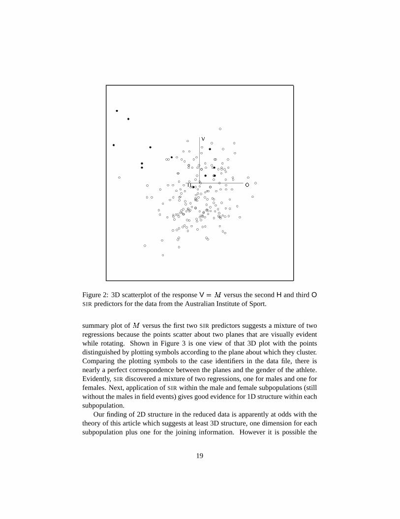
Figure2: 3D scatterplotof theresponseV ÐUÑ versusthesecondH andthird OSIR predictorsfor thedatafrom theAustralianInstituteof Sport.

summaryplot of Ñ versusthefirst two SIR predictorssuggestsa mixture of tworegressionsbecausethe pointsscatterabouttwo planesthat arevisually evidentwhile rotating. Shown in Figure 3 is one view of that 3D plot with the pointsdistinguishedby plottingsymbolsaccordingto theplaneaboutwhich they cluster.Comparingthe plotting symbolsto the caseidentifiers in the datafile, there isnearlya perfectcorrespondencebetweentheplanesandthegenderof theathlete.Evidently, SIR discovereda mixtureof two regressions,onefor malesandoneforfemales.Next, applicationof SIR within themaleandfemalesubpopulations(stillwithout themalesin field events)givesgoodevidencefor 1D structurewithin eachsubpopulation.

Our finding of 2D structurein thereduceddatais apparentlyat oddswith thetheoryof this articlewhich suggestsat least3D structure,onedimensionfor eachsubpopulationplus one for the joining information. However it is possiblethe

19

Ò

Ó

Ô

Figure3: 3D scatterplotof the responseV Õ×Ö versusthe first H andsecondOSIR predictorsfor thedatafrom theAustralianInstituteof Sportwithout malesinfield events.

centralsubspacefor themaleregressionis quite closeto thecentralsubspaceforthe femaleregression. If this wereso, SIR might well find 2D structure,with acommon1D subspacefor thetwo intra-genderregressionsplusa 1D subspaceforthejoining information.Furtheranalysissustainsthis possibility. For example,intheoriginal Ø -scale, Ù

Õ�Ú)ÛVarÜ�ÝßÞ,à�áãâ)ÜVäåãæ^ç+èêé^ë äå�ìíédæ^ç+èêé Þis anestimateof thecoefficient vectordeterminingtheoptimallinearcombinationîIïð Ý of thepredictorsfor discriminatingbetweenmaleandfemaleathletes.Theñ�ò

value from the OLS regressionof

Ù ï Ý on the first two SIR predictorsfromthe regressionin the combinedpopulationis about0.99. Thus, the SIR analysisessentiallyrecovers the optimal linear combinationwithout direct knowledgeof

20

theindividual subpopulations.Thatleavesonecommondimensionto describetheintra-genderregressions.

Thisexampleillustratestheability of themethodologyto identify sequentiallypotentiallyrelevantsubpopulations.Interpretationswererelatively straightforwardbecausethereis informationon thecasesin thedatafile to supportthefindingsofSIR. Thenext examplelackssuchinformation.

7.2 SwissBank Notes

Flury andRiedwyl (1988,p. 5) gave a dataseton counterfeitSwissbanknotes.Theresponsevariableis anote’s authenticity, ó�ô�õ for genuinenotesand ó�ôUöfor counterfeitnotes.Thereare6 predictors,eachgiving a differentaspectof thesizeof a note: lengthof bottomedge,diagonallength,left edgelength,lengthatcenter, right edgelengthandtopedgelength.

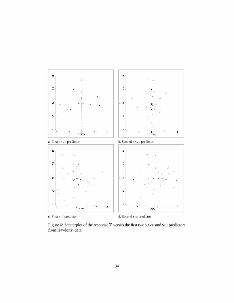
Applying SIR to the bank note datayields the summaryplot shown in Fig-ure 4. The plot is of thefirst SIR predictor ÷ùø�úüû versusthesecondSIR predictor÷ýø�úXþ with thepointsmarkedaccordingto a note’s authenticity. With a binaryre-sponsethereareonly two possibleslices,which meansthat SIR canfind at most1D structure(Cook1996).Becauseof this, thedimensionrepresentedby ÷ýø+úgþ isessentiallynoise. The plot shows goodseparationbetweenthe note typesandapossibleoutlying authenticnote. We next turn to SAVE which revealsadditionalstructure.

SAVE doesnotsuffer from thelimitationsof SIR in thisexample.BecauseSAVE

gainsinformationfrom conditionalcovariancematricesin additionto conditionalmeans,it is not limited to findingatmost1D structure.Applicationof SAVE to thebanknotedatagivesa clearindicationof 2D structure.Thesummaryplot of thefirst two SAVE predictorsis shown in Figure5, againwith pointsmarkedaccordingto a note’s authenticity. The samplecorrelationbetweenthe first SIR and SAVE

predictorsis about0.995sothehorizontalaxesin Figures4 and5 areessentiallythesame.Thedifferencein thesummaryplotsis in thesecondpredictor, which isinformative for SAVE but not informative for SIR.

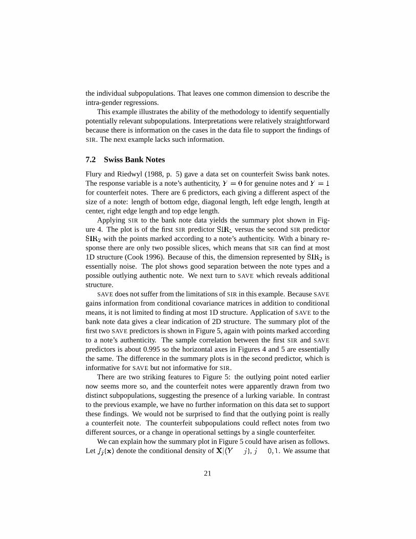
Thereare two striking featuresto Figure5: the outlying point notedearliernow seemsmore so, and the counterfeitnoteswereapparentlydrawn from twodistinctsubpopulations,suggestingthepresenceof a lurking variable. In contrastto thepreviousexample,wehaveno furtherinformationon thisdatasetto supportthesefindings. We would not besurprisedto find that theoutlying point is reallya counterfeitnote. The counterfeitsubpopulationscould reflectnotesfrom twodifferentsources,or achangein operationalsettingsby asinglecounterfeiter.

Wecanexplainhow thesummaryplot in Figure5 couldhavearisenasfollows.Let ÿ�������� denotetheconditionaldensityof ����ó ô ��� , �cô�õ�� ö . We assumethat

21

�������

� ����

���! " ��#� $&% # #' $(% �& ")*

)+-,+ .

)/ ,.

0 ,+ .

1

Figure4: Plotof thefirst two SIR predictorsfrom thebanknotesdata.Opencirclescorrespondto authenticnotes,andblackcirclescorrespondto counterfeitnotes.

24345�6�7is multivariatenormalwith mean 8 3 andcovariancematrix 9 . Following

the indicationsin Figure5, we assumefurther that2�:;5�6�7

is a mixture of normaldensities, 2�:;5�6�7=<?>@2�:A:�5�6�7CB?5!DFEG>H7!2�:JI�5�6�7where

2 :JK 5�6�7is the multivariatenormal densitywith mean 8 :JK and covariance

matrix 9 , L <MD4N'O. The mixing probability

>for the counterfeitnotescould

correspondto a lurking variable. After a little algebra,the regressionoddsratiocanbeexpressedas

P 5RQS<UTWV XY<Z6�7P 5RQS<[D\V XY<Z6�7 < ]_^�`ba 5 8 3 E 8 :A: 7Jc 9ed

: 6Hfg 3 B g : ]_^h`ba 5 8 :JI E 8 :A: 7 c 9 d

: 6Hfwhere g 3 and g : areunknown constantsnot dependingon

6. It follows that the

22

ikjmlonWp

qr stu

v�w!x y v�z'x { z z�x { w&x y|}

|~

�

~

Figure5: Plot of thefirst two SAVE predictorsfrom thebanknotesdatawith thepointsmarkedaccordingto anote’s authenticity, with circlescorrespondingto au-thenticnotes.

regressionof � on � has2D structurewith

�C��� ���[�e�b���F���������G� �A����� ��� �J� �G� �A�-�'�Thetwo vectorsdefiningthis subspacecanbeestimateddirectly from thesubsetsof the datacorrespondingto the threesubpopulationsof Figure5. The resultingestimatedsubspaceis quitecloseto theestimatedSAVE subspace,supportingtheideathat this retrospective reasoningmaysubstantiallyaccountfor thefindingsinFigure5.

Finally, wecanre-expresstheoddsratio as

������� � � �Z�W  � �Z¡ �� � � �£¢\  � �Z¡ �

�U¤ � �@¥§¦©¨ � � � ����� �!¢ ¥§ª_«h¬ ��¤ � ��¥­¦C¨� � �A�

23

which providesa first (nonlinear)logistic modelfor theregression.We doubtthatwewouldhavearrivedatamodelof this form without theguidanceavailablefromFigure5.

7.3 ChallengeData

7.3.1 Hawkins Data

Wenext consideradatasetcraftedby DouglasHawkins(personalcommunication)in 1997asa testcaseto challengetraditionalandrobust regressionmethodswithoutliersbasedon Huber’s (1981,Section8.9) discussionof the breakdown pointfor covariancematrices.Thereare32 casesandfour predictors® ; 24 of thecasescomefrom a primary regression,andthe remaining8 casescomefrom a distinctsecondaryregression.Thesesubpopulationregressionsarecharacterizedby theirrespective meanfunctionsE ¯R°²± ®²³ whicharelinearin thefour predictors.

As expected,the structureof thesedatais not revealedeasilyby usingtradi-tional regressionmethods. For example,two-dimensionalscatterplotsof the re-sponseagainsteachpredictorfail to provide usefulhints aboutthe structureandthe ´¶µ value for the OLS regressionof ° on ® with all 32 casesis only 0.025.However, usingonly thedatafrom theprimaryregression, µ¸·Z¹�º¼»�½ , while usingonly thedatafrom thesecondaryregression¶µ ·Z¹�º¼»�»�»�¾�¿ .

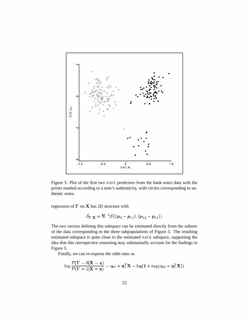
Theplot of ° versusthefirst SAVE predictorshown in Figure6afindsakey partof thestructure.The8 highlightedpointscorrespondto thesecondaryregression.Theremainingpointsfall neara planethat is nearlyvertical to thehorizontalaxisof theplot. This plot is nearlyidenticalto theplot of ° versusall 32 fitted valuesfrom themeanfunctionestimatedby usingOLS on the24 casesfrom theprimaryregression.

The3D plotof ° versusthefirst two SAVE predictorsÁÀ�Â�ÃÅÄFÆ�Ç�À�©ÃÈÄ µ ³ clearlyshows pointsclusteringabouttwo distinctplanesandthusindicatesthattheremaybetwo laws involved. Theplot for thesecondSAVE predictorshown in Figure6bmay help visualizethis 3D plot. The correspondingplots for SIR shown in Fig-ures6cd completelymiss the structureof the problem,the 3D plot of ° versus¯ÁÀhÉ&ÊËÆ�Ç�ÀhÉ&Ê µ ³ suggestingthattheresponseis independentof theSIR predictors.

This exampleenforcesthenotionthat SAVE is moreresponsive to outliersandregressionmixtures. It alsosupportsthe idea that methodsbasedon estimatingthe centralsubspacecan easily handleproblemsthat aredifficult for traditionalmethods.

24

7.3.2 RousseeuwData

Rousseeuw(1984), Atkinson (1994) andothershave usedthe following regres-sion structureas a test casefor robust methods. From a total of ÌSÍÎÌHÏÑÐÒÌCÓcasesÔRÕ�Ö�×ÈØ , Ì Ï areconstructedto follow a simplelinear regressionin predictor× , while the remaining ÌCÓ casesare generatedfrom a secondsubpopulationinwhich Õ × . Observationsfrom thesecondsubpopulationareusuallygeneratedto scatterabouta point of high leveragerelative to thesimplelinear regressioninthefirst subpopulation.Thus,unlike theresponseoutliersdefinedin Section3.4, Ùand × aredependent.A robust methodis judgedto besuccessfulif it revealsthestructureof all Ì cases.

Test casesof this sort are largely coveredby the discussionof Section5.3.Generalizingto Ú predictors,assumethatin onesubpopulationtheregressionof Õon Û is characterizedby its linearmeanfunctionE ÔRÕÝܼÛ�Ö�Ù­Í£Þ;Ø=Í?ß�Ðáàãâ Ï Û , whileÕ ÛäÜ�Ô�ÙåÍ?æ�Ø . Assumingthat çÎÍ?è , which seemsin spirit of therobuststudiesusingexamplesof thissort,wehave from Proposition4 that é E ê�ëíì î©ï�ð éÅÔñà Ï Ö'ò Ï Ø .Further, if thesubpopulationsarenormal,it follows accordingto thediscussionofSection5.3 that é E ê�ëíì î@ï Íóé î�ì ë ÍóéÈÔñà Ï Ö'ò Ï Ø�Íõô . In eithercase,SIR shoulddoagoodjob findingtheunderlingstructure,aconclusionthatis sustainedby asmallsimulationstudynot reportedhere.

8 Discussion

Regressionsoften include outliers, mixtures and other subpopulationstructure.While therearemany methodsfor detectingsuchphenomena,nearlyall rely onsummarizingdeviationsfrom afit of aparametricmodelthatis assumedto becor-rect for themajority of thedata.Thewidely applicableparadigmproposedin thispaperis different. Approachinga regressionthroughits centralsubspaceenablesthe analystto constructlow-dimensionalsummaryplots that may show the mainregressionstructureaswell asoutliersandmixtureswithouttheneedto pre-specifya parametricmodel.Thesummaryplot thenallows a low-dimensionalview of thedatathat is not fetteredby a model. On the contrary, this may often lead to aninitial parametricmodel.

Residuals. All of themethodsandideasdiscussedin this articleareapplicablewhentheresponseÕ is replacedby aresidualö from thefit of aparametricmodel.The usefulnessof an analysiswith residualscandependon the relationbetweené î�ì ë andthe correspondingcentralsubspaceéb÷ ì ë for the regressionof ö on Û .ResidualsaremostusefulwhenøWùûú²Ô�é ÷ ì ë Øãü�ømùûú²Ô�é î�ì ë Ø . Ontheotherhand,when

25

ýmþûÿ�������� ���åýmþûÿ���� ��� ��useof residualscancomplicateananalysisunnecesarily.

Theseandotherresultsgiven by Cook (1998a;1998b)on the useof residualsinpursuitof centralsubspacesareapplicablein thecontext of thisarticle.

Visualization. Formal parametricteststhat specificallytarget outliers or othersubpopulationstructurearenot requiredin this paradigm.Instead,the analystisfree to follow visual impressionsfrom the estimatedsufficient summaryplot toguide subsequentanalysis,much like viewing a 2D plot of the responseversusthe predictor in a simple regressionproblem. In our experience,this ability toassessregressionsin a low-dimensional,model-freecontext often leadsto resultsthat would have beenquite difficult to find usingmore traditionalmethods.Forexample,in the banknoteregressiondiscussedin Section7.2, visual analysisofthe SAVE summaryplot in Figure5 suggesteda nonlinearlogistic modelwith 2Dstructure. And our analysisof the Hawkins dataidentified the main regressionstructurein aproblemthatwasdesignedto challengetraditionalmethods.

Sequentialmethods. We restricteddiscussionto only two distinct subpopula-tions for the formal developmentsin this article. Thereis no loss of generalityimplied by this restrictionbecauseeitherof thetwo subpopulationscoulditself becomposedof multiple subpopulations.Complicatedmultiple subpopulationstruc-ture canoften be sortedout sequentiallyby temporarilydeletingoutliersor setsof casesthatcanbelinkedto recognizablesubpopulations.This wasillustratedinthe AustralianSport regressiondiscussedin Section7.1. This ability to analyzea regressionsequentiallyseemsuniqueto thisparadigmbecausedeletingobserva-tionsfrom onesubpopulationdoesnoteffectthecentralsubspacefor theremainingsubpopulations.

Theability to proceedingsequentiallycanbeimportantif thereareseveralsub-populationspresentbecausethenthestructuraldimensionof the regressioncouldbeat its maximum� . Suppose,for example,thatwe areusingSAVE in a problemwith severaloutlierscausingahighstructuraldimension.SAVE will tendto find themostoutlying point(s)in its first oneor two directions.Sequentiallydeletingsuchpointsfollowedby reapplicationof SAVE canbeexpectedto reducethestructuraldimensionuntil themainregressionstructurerisesto thesurface.

SAVE and SIR. Oneconclusionof this article is that the centralsubspacepro-videsa uniquehandleon regressionoutliersandmixtures. However, methodsofestimatingthe centralsubspacearerequiredfor implementation.We consideredonly two methods– SIR andSAVE – in this articlebecauseour investigationshaveshown thatthey canbequiteusefulin application.Nevertheless,othermethodsare

26

available. In additionit maybepossibleto tailor methodsfor thespecifictaskofidentifying outliersandmixtures.Work alongtheselinesis in progress.

9 Appendix: Justifications

Someof thejustificationsin thisappendixmake useof thefollowing lemma.

Lemma 1 Let ��� bea dimension-reductionsubspacefor theregressionof � on � ,andlet � ��� � � . Then � � is a dimension-reductionsubspacefor theregressionof� on � .

Justification: The conclusionfollows immediatelyfrom the following generalresult (see,for example,Dawid 1979). Let � , � and � be randomvectors,and let ��� be a (measurable)function of � . Then � ��� � implies that� ��� ���"!#���%$ .

Proposition 1. The following pair of conditions & � and &'� is equivalent to thepairof conditions( � and ()� (seeDawid 1979;or Cook1998b,p. 64).

�*&+�,$-� �.� �0/213�4!657$8�*& � $9� 5:� /313��6( � $ � 5;� �0/ 1 �4!#�<$8�6()�=$ � �>� / 1 �Taking /-? �A@7BC!D@ � !D@ � $ , conditions �*&+�,$ and �*& � $ hold by constructionandLemma1. Theconclusionthenfollows from condition �6(,�=$ .

Proposition 2. As in Section3.2, let E�FHGI?J� K�L MINO�:�A@ F $�NO���A@ G $ . Considerfirst thecasewhere ��PQ!SRT!QUV$�?W�*XY![ZC!Q\]$ sowe needto show that ���A@ B $ � E^� � . Let_ bea basisfor ���A@4B=$a`.E � � , andextend _ to bases� _ !Qbc$ for ���A@4B=$ and � _ !edc$for E^� � sothat �:� _ !edc$3?f� KgL M �A@^$�Nh���A@ � $ Ni���A@ � $In particular, eachof � KgL Mj�A@^$ , �:�A@ � $ and �:�A@ � $ is a subspaceof ��� _ !edc$ . ByLemma1, we may thereforesubstitute � _ !edc$ for eachof @ , @ � and @ � in (4).UsingLemma1 again,wemayalsosubstitute� _ !Qb�!ed+$ for @4B in (4). Substitutingandrearranging,wefind

k �*�Jlnm�� _ 1 �4!ed 1 ��$o? k �*�plqm � _ 1 �4!ed 1 �4!65r?s\]$aNk �t5h?uZv� _ 1 �7!ed 1 �4!Qb 1 ��$xw B ��mc!y��$ (23)

27

where

z�{T|�}�~y���2����|*�p�q} � ���3�7~e�'�3�4~6�h�u�=������|*���q} � ���3�4~e�'�3�4~6�h�s�]�Taking the expectationof both sidesof (23) over the conditionaldistribution of� �3��� |6� � �7~e�'�3���

andsubtractingtheresultfrom (23)gives� ��|t�n���v� ���3�4~e�'�3�7~ � �3���j����|t�h���v� ���3�4~e�Y�3���Q����z:{]|�}�~y�g�g�f�Thus,as� |6��~e�+�

is adimension-reductionsubspacewithin eachsubpopulationand��|*��{%�g���, it follows that�=� � ��|t��� �v� ���3�r�f��� � ~e�'�2�i���'� � ~ � �3�r� � � � �2�

��|t�q���v� � � �i�s� � � ~e� � �i��� � � �Q�(24)

hasprobability one. But � |A¡ { ��� � |6��~ � �is the centralsubspacefor the re-

gressionof�

on�

. Thus, (24) gives � |6�¢~ � �¤£ � |6��~e�c�which is the desired

conclusion.The proof is similar in thecasewhere

|�¥#~S¦]~Q§V�¢�¨|D�C~#�Y~Q�]�. Interchangingthe

subscripts0 and1 in re-defining|6��~ � ~e�+�

andarguingasabove,substitutionin (4)hereyields:

��|*�p�q} � � � �4~e� � �g�©� ��|t�h���v� � � �4~e� � ���7���|*�p�q}�� � � �4~e� � �4~ � � �4~6�h���=�aª

��|t�h�s�V� ���3�4~e�'�3���7���|*�p�q}�� �^�3�4~e�Y�3�4~6�r�s�]�

(25)

Takingtheexpectationof bothsidesof (25) with respectto theconditionaldistri-bution of

� � ��� |6� � �4~e� � �7~6�q���=�andsubtractingtheresultfrom (25)gives� ��|*���q}�� �^�3�4~e�Y�3�4~ � �3�4~6�h���=�3����|*���q}�� �^�3�4~e�'�3�4~6�h���=�Q�=z¢«¬|­���2���

wherez�«=|­���>�®��|t�¯�o�v� � � �4~e�'�3���

. Thus,as � |6��~e�+�is herea dimension-

reductionsubspacefor theregressionof�

on�

and��|*�°«��2���

, theset�=� � ��|*���q} � ���3�i�s��� � ~e�±�3�r�f�±� � ~ � �3�r� � � � ~6�n���=�2���|*���q} � ���3�i�s�^� � ~e�Y�3�i���'� � ~6�n���=�Q�

(26)

hasprobability one. But here � |A¡ « �.� � |6��~ � �is the centralsubspacewithin

the�u�²�

population.Thus,(26) gives � |6��~ � �³£ � |6��~e�+�which is the desired

conclusion.Thefinal case

|�¥Q~S¦T~Q§�~)���u|6�'~#�Y~[�=�follows by symmetry.

28

Proposition 4.

E ´­µ�¶ ·<¸o¹ Eº�» ¼�½ E ´­µ�¶ ¾^¿#·À¸QÁ¹ Eº�» ¼ ½ E Âô­µ�Ä E ´­µ�¶ ¾7¸e¸�¶ ¾�¿#·°ÅÇÆ E ´­µ�¶ ¾7¸QÁ¹ Eº�» ¼ ½ E Âô­µ�Ä E ´­µ�¶ ¾7¸e¸�¶ ¾�¿#·°Å6Á4Æ Eº�» ¼ ½ E ´­µ�¶ ¾7¸QÁ (27)

It is straightforwardto verify that

Eº�» ¼ ½ E ´­µ^¶ ¾4¸QÁ:¹È½ É ´t¾n¹�Êv¶ ·<¸jÄÌËÊ�ÄÌË Á%Í�Î^Ï>Ð º�» ÑTurningto thefirst termof (27), it follows from thelinearityof E ´­µ^¶ Ò7ÓÔ�µ4¿6¾r¹Õ ¸ andProposition3, Part1, thatfor

Õ ¹�ÊC¿QÖE Âô­µ�Ä E ´­µ�¶ ¾h¹ Õ ¸e¸�¶ ¾q¹ Õ ¿#·°Å�¹È× Ô Ò Ô­Ø Ô ´*·<¸ (28)

where Ø Ô ´*·À¸ is a columnvector that may dependon the valueof · . A similarresultwasalsoshown by Cook(1998b,Proposition10.1).

Next, usingthe two assumedconditionson µ�¶ Ò Ó Ù µ , it follows from Proposi-tion 3, Part2, that Ð:´*Ú¢Äh× Ô ¸7ÛqÐ+º�» Ñ ,

Õ ¹�ÊC¿QÖ . Thus,reasoningfrom (28),

E Âô­µ�Ä E ´­µ�¶ ¾h¹ Õ ¸e¸�¶ ¾n¹ Õ ¿#·�Åܹ Ò Ô Ø Ô ´*·<¸jÄ�´*Ú�Äh× Ô ¸SÒ Ô Ø Ô ´*·À¸Ï Ð:´AÒ4Ô­¿#Ú¢Äh× Ô ¸

Usingthiswith (27)we have

E ´­µ�¶ ·<¸ Ï Ð:´AÒ Î ¿DÒ�ݬ¿#Ú¢Äh× Î ¿#Ú�Är× Ý ¿QÍ Î ¸¹ Ð:´AÒ�Î�¿DÒ Ý ¸ ÆrÐ�´ßÞq¿QÍ�Î)¸

thesecondrelationfollowing from (13).

Proposition 5.

Ú�Ä Var­µ�¶ ·<¸3¹ Eº�» ¼ ½=Ú¢Ä Var­µ�¶ ¾^¿#·À¸QÁ�Ä Varºc» ¼ ½ E ´­µ^¶ ¾�¿#·³¸QÁ (29)

Theconclusionwill follow if we show thatthespansof thetwo termson therightof thisequationsatisfytherequiredinclusion.

ForÕ ¹àÊC¿QÖ , sinceE ´­µ�¶ Ò7ÓÔ µ4¿6¾á¹ Õ ¸ is linear, we canapply Proposition3

within subpopulationÕ

to concludethat

E ´­µ�¶ ¾h¹ Õ ¿#·<¸7Ï>Ð Ô¼g» Ñ29

andthus â:ãVarä�å æ�ç E

ã­è�é ê^ë#ìÀíQî¬í4ïqâ^ðægå ñ³ò â�óægå ñTurningto thefirst term,let ô ã�õ#ë#ì�í3ö

Varã­÷<ø ð­ùDóú è�é ûÀö�õ#ë#ìÀí

. Thenû�üVar

ã­è^é êqö�õ#ë#ì<í©ö û¢üh÷ ð­ùDóú ô ã�õ#ë#ì<íQ÷ ð­ùDóúö ã*û�üh÷ ú í ò ÷Àø ð­ùDóú ã*û�ü ô ã�õ#ë#ì<íeíQ÷ ð­ùDóúü¢ã*û�üh÷ ú íQ÷ ø ð­ùDóú ã*û¢ü ô ã�õ#ë#ì�íeíQ÷ ð­ùDóúThefirst andthird termsin thisfinal expressionarein

â äcå ñ by Proposition3,Part2,usingthetwo assumedconditionson

è�é ý�þÿjè. Thesecondtermis in

â úæ�å ñ becauseby Proposition3 â:ã*û¢ü ô ã�õ#ë#ì�íeí4ïqâ úægå ÷�� ������ ñandthus

÷ ø ð­ùDóú ã*û�ü ô ã�õ#ë#ì<íeí7ïnâ úægå ñ . It follows thenthatâ:ãEä�å æ ç û¢ü

Varã­è^é ê�ë#ì³íQî¬í4ïqâ ðægå ñÀò â óæ2å ñÀò â ä�å ñ

Proposition 6. Let÷ ñ å�æ ö

Varã­è^é�ìÀí

and �� ö���ã�ì¯ö��Ví����, where

ìhas

samplespaceç�� ë ����� ë��iî. Because

èis standardized

EãE

ã­è�é ìÀíeígö �� � ð �� E

ã­è�é ìuö!�Ví2ö"�(30)

and û³öE

ã­÷ ñ å �æ í ò VarãE

ã­è^é�ìÀíeí(31)

Using(30), thesecondtermon theright handsideof (31) is

VarãE

ã­è�é ìÀíeí2ö �� � ð �� E

ã­è^é ìuö!�VíE

ã­è^é ìuö!�VíSþ

Hence,

�� � ð �� E

ã­è�é ìuö#�VíE

ã­è�é ì�ö!�Ví þ ö �� � ð ��

ã*û�üh÷ ñ å $ �æ % �& í (32)

Changingspanningrepresentations,and using (32) and (30), the SAVE sub-spacecanbesuccessively expressedasâ(' $ ñ å�æ & ö â*)

Eã*û�üh÷ ñ å�æ í ó,+

30

- .*/ 0214365%7 8,9:<;>=@?BA�C�C�CDA 0214365%7 8,9:(;FEG?IH- .*/ EJK ;>=�L K E M@NPO�QR -#SUT E M@NPO�QR -#SUT�V A�W = A�C�C�CDA�W EPXF= H- .*/E M@NPO�QR -ZYDT A�C�C�C[A E M@NPO�QR -!\]1^YDT A�W = A�C�C�C�A�W EPXF= H

whereW K -�365%7 8 9:(; K�_ =@? 1`365%7 8 9:(; K ? , Sa-bY A�C�C�CDA \�1cY . Therequiredresultnowfollows.

References

Atkinson, A. C. (1994). Fastvery robust methodsfor the detectionof multipleoutliers.Journalof theAmericanStatisticalAssociation, 89,1329–1339.

Box, G. E. P. (1966).Useandabuseof regression.Technometrics, 5, 141-160.

Cook,R. D. (1992a).Graphicalregression.In Dodge,Y. andWhittaker, J. (eds),ComputationalStatistics, Vol. 1. New York: Springer-Verlag,11–22.

Cook, R. D. (1994a). On the interpretationof regressionplots. Journal of theAmericanStatisticalAssociation, 89,177–190.

Cook,R. D. (1994b).Usingdimension-reductionsubspacesto identify importantinputsin modelsof physicalsystems.In 1994Proceedingsof theSectiononPhysicalEngineeringSciences, Washington.

Cook,R. D. (1996).Graphicsfor regressionswith a binaryresponse.Journal oftheAmericanStatisticalAssociation, 91,983–992.

Cook, R. D. (1998a). Principal Hessiandirectionsrevisited (with discussion).Journalof theAmericanStatisticalAssociation, 93,84–100.

Cook,R.D. (1998b).RegressionGraphics:Ideasfor studyingregressionsthroughgraphics. New York: Wiley.

Cook,R.D. andLee,H. (1999).Dimensionreductionin regressionswith abinaryresponse.Journalof theAmericanStatisticalAssociation, 94,1187–1200.

Cook, R. D. andLi, B. (1999). Dimensionreductionfor the conditionalmean.Submitted

Cook,R. D. andNachtsheim,C. J. (1994). Re-weightingto achieve ellipticallycontouredcovariatesin regression.Journal of theAmericanStatisticalAs-sociation, 89,592–599.

31

Cook, R. D. andWeisberg, S. (1991). Discussionof Li (1991). Journal of theAmericanStatisticalAssociation, 86,328–332.

Cook,R. D. andWeisberg, S. (1994). An Introductionto RegressionGraphics.New York: Wiley.

Cook,R. D. andWeisberg, S. (1999). AppliedRegressionIncludingComputingandGraphics. New York: Wiley.

Cook,R. D. andWetzel,N. (1993).Exploringregressionstructurewith graphics(Invited with discussion).TEST, 2 ,1–57.

Cook,R. D. andYin, X. (1999).Dimensionreductionfor the d th moment.Sub-mitted.

Dawid, A. P. (1979).Conditionalindependencein statisticaltheory(with discus-sion).Journal of theRoyalStatisticalSociety, SerB., 41,1–31.

Diaconis,P. andFreedman,D. (1984). Asymptoticsof graphicalprojectionpur-suit. Annalsof Statistics, 12,793–815.

Flury, B. andRiedwyl,H. (1988).Multivariate Statistics:A PracticalApproach.London:ChapmanandHall.

Hall, P. andLi, K. C. (1993).On almostlinearity of low dimensionalprojectionsfrom highdimensionaldata.Annalsof Statistics, 21,867–889.

Huber, P. (1981).RobustStatistics. New York: Wiley.

Joiner, B. L. (1981). Lurking variables:Someexamples.TheAmericanStatisti-cian, 35,227–233.

Li, K. C. (1991).Slicedinverseregressionfor dimensionreduction(with discus-sion).Journal of theAmericanStatisticalAssociation, 86,316–342.

Li, K. C. (1992). On principal Hessiandirectionsfor datavisualizationanddi-mensionreduction: Anotherapplicationof Stein’s lemma. Journal of theAmericanStatisticalAssociation, 87,1025–1039.

Moore,D. S.(1997).Statistics,ConceptsandControversies,fourthedition.NewYork: FreedmanandCompany.

Rousseeuw, P. J. (1984). Leastmedianof squaresregression. Journal of theAmericanStatisticalAssociation, 79,871–880.

32

Sheather, S. andMcKean,J. W. (1997). A comparisonof proceduresbasedoninverseregression.In Y. Dodge(ed.),L1 StatisticalProceduresandRelatedTopics: IMSLecture Notes,Vol 31,271–278.

33

e@f�gih,j

k

l m l n o n mpqsrtuvupsrtu w

x@y�zi{�|

}

~ � ~ � � � ���s������s��� �

a. First SAVE predictor b. SecondSAVE predictor

�@���i�

�

� � ��� � � � ���s������s��� �

�@�����

 

¡ ¢ ¡ £ ¡�¤ ¥ ¤ £¦§s¨©ª«ª¦s¨©ª ¬

c. First SIR predictor d. SecondSIR predictor

Figure6: Scatterplotof theresponse­ versusthefirst two SAVE andSIR predictorsfrom Hawkins’ data.

34