Identifying Protein Interactions Amongst DNA Damage Repair Proteins in Yeast

by

Siyang Li

A thesis submitted in conformity with the requirements for the degree of Master of Science

Molecular Genetics University of Toronto

© Copyright by Siyang Li 2014

ii

Identifying Protein Interactions Amongst DNA Damage Repair Proteins

in Yeast

Siyang Li

Master of Science

Molecular Genetics University of Toronto

2014

Abstract Mapping protein-protein interactions (PPIs) is crucial for understanding cellular systems.

PPIs can be studied with binary or co-complex methods. A major economical binary method is

the yeast two-hybrid (Y2H) system. However, current Y2H is still very time-consuming for

studying large protein matrices. Here, I applied a new technology developed in our lab, Barcode

Fusion Genetics Yeast Two-Hybrid (BFG-Y2H), to study ~69,000 protein pairs amongst 263

yeast DNA damage repair proteins. BFG-Y2H combines Y2H, DNA-barcoding, barcode-fusion

genetics and next-generation sequencing to increase the current throughput of Y2H. I

demonstrated that BFG-Y2H screens are reproducible and of comparable quality to a previously

published high-quality Y2H dataset. In addition, I also discovered and confirmed five novel Y2H

interactions amongst the top scores with the BFG-Y2H screens when compared to all previously

published literature. Thus, BFG-Y2H can be used to more efficiently capture PPIs.

iii

Acknowledgments

Foremost, I want to express my sincerest gratitude to my supervisor, Dr. Frederick Roth,

for providing patient guidance, supportive mentorship and an excellent work environment during

my M.Sc. studies. In addition to teaching me the subjects of high-throughput biology, he has also

indirectly taught me on how to be a generous, forgiving and kind person by setting such an

excellent example. It has been a great privilege and pleasure to work under his supervision for

the past two and a half years.

I want to also thank my committee members, Dr. Amy Caudy and Dr. Alex Ensminger,

for the helpful guidance, valuable suggestions and continuous mental support to complete my

project. Their support has been invaluable to me.

I am truly grateful for the help and support of my lab-mates and collaborators. I am

indebted to Dr. Nozomu Yachie for training me as a high-throughput biologist and for setting an

excellent example of a great scientist. I am extremely grateful to Dr. Evangelia Petsalakis for her

continuous support on everything, especially data analysis, and her friendship, which has made

the hardest times much easier. I want to thank Dr. Javier Diaz for helping me to select the genes

for my project. I want to thank Dr. Atina Cote and Dr. Joe Mellor for sharing their knowledge of

yeast biology and sequencing with me. I am grateful to Takafumi for all of his patient

mentorship and advice on sequencing analysis and Jochen for his patience in answering my R

questions. I want to thank Marta and Analyn for their technical support in the lab and Nidhi from

the Vidal lab for providing clones for my project. I am thankful to the rest of the Roth lab,

especially Marinella, Song and Mariana for providing warm friendships and support for the last

couple of years. I would also like to thank Dr. Corey Nislow and his lab at the University of

Toronto for providing guidance and support for the first year of my graduate studies.

I want to thank my friends, Gowtham, Kirill, Tetyana and Victoria for being my support

system, both personally and scientifically.

Finally, and most importantly, I want to thank my parents and Walter for their endless

understanding, support, patience and love during my MSc studies.

iv

Table  of  Contents  

Acknowledgments  .................................................................................................................................  iii  

List of Tables  ..........................................................................................................................................  vi  

List of Figures  ........................................................................................................................................  vii  

  Introduction  ...................................................................................................................................  1  1

1.1   Mapping  protein-­‐protein  interactions  .......................................................................................  1  

1.2   Yeast  two-­‐hybrid  ...............................................................................................................................  2  

1.3   Limitations  and  advantages  of  the  classical  Y2H  method  ...................................................  4  

1.4   Quality-­‐control  for  Y2H  and  recent  advances  .........................................................................  5  

1.5   Overview  of  Barcode  Fusion  Genetics  Yeast  Two-­‐Hybrid  (BFG-­‐Y2H)  .............................  7  

1.6   BFG-­‐Y2H  helps  to  uncover  novel  interactions  amongst  DNA  damage  repair  proteins

  9  

  Materials  and  Methods  ............................................................................................................  10  2

2.1   Barcode-­‐Fusion  Genetics:  background  strains  ....................................................................  10  

2.2   Generation  of  barcoded  destination  vectors  ........................................................................  13  

2.3   Selection  of  DNA  damage  repair  proteins  ..............................................................................  16  

2.4   Generating  barcoded  Y2H  strains  .............................................................................................  20  

2.5   BFG-­‐Y2H  screens  ............................................................................................................................  23  

2.6   Replicates  for  the  BFG-­‐Y2H  screens  .........................................................................................  25  

2.7   Pairwise  retesting  ..........................................................................................................................  28  

2.8   Calculation  of  interaction  scores  ..............................................................................................  29  

2.9   Statistical  analysis  and  datasets  used  .....................................................................................  30  

  Results  ..........................................................................................................................................  31  3

3.1   Reproducibility  of  the  BFG-­‐Y2H  screens  ................................................................................  31  

3.2   Positive  controls  in  the  BFG-­‐Y2H  screens  ..............................................................................  38  

3.3   Untangling  positive  controls  ......................................................................................................  45  

3.4   BFG-­‐Y2H  screens  ............................................................................................................................  47  

3.5   Benchmarking  for  pairwise  retesting  .....................................................................................  54  

3.6   Pairwise  retesting  on  BFG-­‐Y2H  candidate  interactions  ....................................................  58  

  Discussion  ....................................................................................................................................  62  4

4.1   Reproducibility  of  BFG-­‐Y2H  ........................................................................................................  62  

v

4.2   Positive  controls  in  the  BFG-­‐Y2H  screens  ..............................................................................  64  

4.3   BFG-­‐Y2H  screen  and  pairwise  retesting  results  ..................................................................  65  

4.4   Novel  interactions  by  pairwise  retesting  ...............................................................................  66  

  Conclusions  and  future  directions  ......................................................................................  69  5

  References  ...................................................................................................................................  70  6

  Appendices  ..................................................................................................................................  75  7

7.1   Arrangement  of  barcode  sequences  on  the  plasmid  ..........................................................  75  

7.2   Barcode  fusion  products  after  the  induction  of  Cre  ...........................................................  76  

7.3   Using  an  en  masse  Gateway  LR  reaction  to  generate  barcoded  strains  .......................  77  

7.4   Pairwise  Resting  of  PRS  ................................................................................................................  82  

7.5   Top  200  interactions  in  the  BFG-­‐Y2H  (-­‐His  condition)  ......................................................  84  

vi

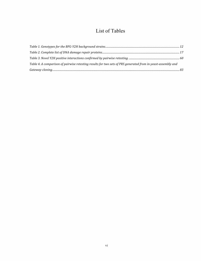
List of Tables

Table  1.  Genotypes  for  the  BFG-­‐Y2H  background  strains.  ................................................................................................................  12  Table  2.  Complete  list  of  DNA  damage  repair  proteins.  .....................................................................................................................  17  Table  3.  Novel  Y2H  positive  interactions  confirmed  by  pairwise  retesting.  .............................................................................  60  Table  4.  A  comparison  of  pairwise  retesting  results  for  two  sets  of  PRS  generated  from  in-­‐yeast-­‐assembly  and  

Gateway  cloning.  .................................................................................................................................................................................................  83  

 

vii

List of Figures Figure  1.  Yeast  two-­‐hybrid  (Y2H).  ______________________________________________________________________________________  3  Figure  2.  Barcode  Fusion  Genetics  Y2H  (BFG-­‐Y2H).  ___________________________________________________________________  8  Figure  3.  Activation  of  Cre  recombinase  in  our  background  Y2H  strains.  ___________________________________________  11  Figure  4.  Generation  of  barcoded  destination  vectors.  _______________________________________________________________  14  Figure  5.  Row-­‐column-­‐plate  PCR  (RCP  PCR).   _________________________________________________________________________  15  Figure  6.  Gateway  LR  reaction  between  a  barcoded  destination  vector  and  an  entry  clone.  _______________________  22  Figure  7.  Assessing  the  reproducibility  of  BFG-­‐Y2H.  __________________________________________________________________  26  Figure  8.  Replicates  within  the  BFG-­‐Y2H  screen.   _____________________________________________________________________  27  Figure  9.  Reproducibility  of  BFG-­‐Y2H  between  two  internal  replicates.  _____________________________________________  32  Figure  10.  Reproducibility  of  BFG-­‐Y2H  between  two  biological  strain  replicates.  __________________________________  34  Figure  11.  Reproducibility  of  BFG-­‐Y2H  between  two  screen  replicates.  _____________________________________________  36  Figure  12.  Reproducibility  of  BFG-­‐Y2H  between  two  screen  replicates.  _____________________________________________  37  Figure  13.  Expected  positive  interactions  for  BFG-­‐Y2H.  ______________________________________________________________  39  Figure  14.  Positive  controls  of  the  BFG-­‐Y2H  screen  in  the  presence  of  histidine  (+His).  ____________________________  41  Figure  15.  Raw  barcode  counts  of  positive  controls  of  the  BFG-­‐Y2H  screen  without  histidine  supplements.  ______  42  Figure  16.  Normalized  scores  of  positive  controls  of  the  BFG-­‐Y2H  screen  without  histidine.   ______________________  43  Figure  17.  Normalized  scores  of  positive  controls  of  the  BFG-­‐Y2H  screen  without  histidine  and  in  the  presence  of  

3-­‐amino-­‐1,2,4-­‐triazole  (+3AT).  ________________________________________________________________________________________  44  Figure  18.  Readjusted  positive  controls  for  the  BFG-­‐Y2H  screens  without  histidine.  _______________________________  46  Figure  19.  Marginal  counts  of  the  BFG-­‐Y2H  screen  without  histidine  supplements.  ________________________________  48  Figure  20.  Distribution  of  marginal  abundance  of  DB-­‐X  and  AD-­‐Y  in  +His.  _________________________________________  49  Figure  21.  Normalized  scores  of  the  BFG-­‐Y2H  screen  without  histidine  supplements.  ______________________________  50  Figure  22.  Normalized  scores  of  the  BFG-­‐Y2H  screen  without  histidine  supplements  and  in  the  presence  of  3-­‐

amino-­‐1,2,4-­‐triazole  (+3AT).   __________________________________________________________________________________________  51  Figure  23.  The  expected  interactome.  _________________________________________________________________________________  52  Figure  24.  The  expected  interactome.  _________________________________________________________________________________  53  Figure  25.  Prediction  performance  of  the  reported  BFG-­‐Y2H  positive  protein  interactions  for  the  –His  condition  

benchmarked  against  Yu  et  al.  43.  ______________________________________________________________________________________  55  Figure  26.  Prediction  performance  of  the  reported  BFG-­‐Y2H  positive  protein  interactions  for  the  –His  condition  

benchmarked  against  all  previous  BioGRID  Y2H  data.  _______________________________________________________________  57  Figure  27.  Pairwise  retesting  results  of  the  top  scores  from  the  BFG-­‐Y2H  screens.  _________________________________  59  Figure  28.  Interactome  of  the  top  200  scored  interactions  from  the  BFG-­‐Y2H  screen  (-­‐His  condition).  ___________  61  Figure  29.  Overview  of  en  masse  Gateway  LR.  ________________________________________________________________________  80  Figure  30.  Results  of  en  masse  Gateway  LR  of  a  pooled  barcoded  destination  vectors  and  a  pool  of  entry  vectors  

containing  94  different  yeast  ORFs  of  lengths  between  200-­‐2900bp.  ________________________________________________  81  

1

Introduction 1

1.1 Mapping protein-protein interactions

Proteins mediate many functions within the cell and interactions between them regulate

the systems-level behavior of cells. As such, mapping protein-protein interactions (PPIs) is

crucial for understanding cellular systems of an organism of interest.

Since the release of the complete genome sequence of the model organism

Saccharomyces cerevisiae in 19961, functional annotations for predicted gene products have

exploded. Given that most proteins require physical interactions with other proteins to fulfill

their biological role, it was proposed that functional annotations for proteins can be obtained by

systematically identifying potential PPIs2. In an effort to accelerate functional annotations of

proteins, many innovative methods for the identification of PPIs have been presented and several

of these methods are currently in use in laboratories around the world3,4 .

There are two general classes of methods for detecting PPIs: those that detect co-

complexed proteins and those that detect binary interactions. An example of a co-complex

method is tandem affinity purification coupled to mass spectrometry5, which determines the

protein components of a complex for a tagged protein of interest by pulling it down from a cell

lysate along with proteins in the same complex and identifying these proteins with mass

spectrometry. In some instances, complexes such as the ribosome have been purified and

analysed directly in the mass spectrometer6. An example of a binary method is the yeast two-

hybrid (Y2H) method (see Section 1.2 for more information) where physical binary interactions

between two proteins are captured. The interaction between Ras and the protein kinase Raf was

2

first detected by Y2H7 and later demonstrated in mammalian cells8. We now know that Ras and

Raf are part of a very important signaling pathway that causes many types of cancer when

misregulated9–12, and have therefore, become the focus of cancer therapy13–15. Many

pharmacological solutions, such as sorafenib16, have been developed and used clinically to

inhibit overly active Raf kinases. This is one of many examples where studying PPIs have not

only improved our understanding of molecular biology but have also led to therapeutic

outcomes.

Even though many innovative methods for the identifying PPIs have been presented,

Y2H is one of the very few methods that can be practically adapted for high-throughput strategy.

1.2 Yeast two-hybrid

Yeast two-hybrid (Y2H) is a major strategy for identifying direct binary protein-protein

interactions (Figure 1). In Y2H, the activation domain (AD) and DNA-binding domain (DB) of a

transcription factor are separated and fused to proteins of interest, Y (also known as “prey”) and

X (also known as “bait”). This results in haploid yeast cells with plasmids that carry AD-Y or

DB-X fusion proteins, which are targeted to the yeast nucleus by nuclear localization signals.

When haploid cells containing AD-Y and DB-X plasmids are mated together, the resulting

diploid cell will contain both AD-Y and DB-X plasmids. Physical interaction between AD-Y and

DB-X will reconstitute the transcription factor and allow transcription of the reporter gene. In the

case of using histidine as a selectable marker, a physical interaction between AD-Y and DB-X

permits the survival of the diploid cell on media without histidine.

3

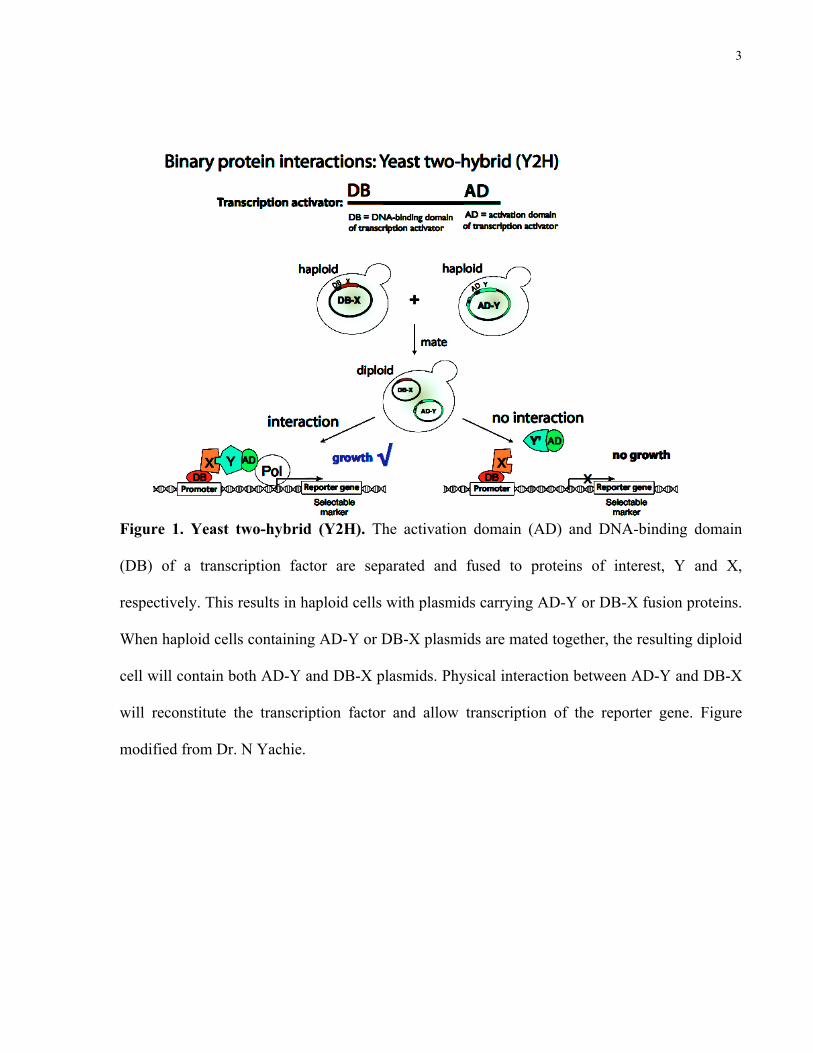
Figure 1. Yeast two-hybrid (Y2H). The activation domain (AD) and DNA-binding domain

(DB) of a transcription factor are separated and fused to proteins of interest, Y and X,

respectively. This results in haploid cells with plasmids carrying AD-Y or DB-X fusion proteins.

When haploid cells containing AD-Y or DB-X plasmids are mated together, the resulting diploid

cell will contain both AD-Y and DB-X plasmids. Physical interaction between AD-Y and DB-X

will reconstitute the transcription factor and allow transcription of the reporter gene. Figure

modified from Dr. N Yachie.

4

1.3 Limitations and advantages of the classical Y2H method

Like every method, Y2H has trade-offs. Since the fusion proteins in the classical Y2H

method are all targeted to the nucleus, they must be able to fold and exist stably in order to retain

their activity. Fusion proteins may also change the proteins’ native conformations, which may

alter their activity and/or binding. Studying the PPIs of the fusion proteins in both directions

(DB-X/AD-Y and DB-Y/AD-X) would help to partially circumvent this problem. The readout of

Y2H is dependent on the reporter’s response to transcriptional activation; therefore, it is possible

that a DB fusion protein could activate transcription on its own (autoactivation). Fortunately, this

can be dealt with by implementing proper controls in the experiment17. However, the most

important concern is the biological relevance of two positive Y2H interactors: due to both time

constraints and cellular localization, two proteins that do not interact under regular cellular

contexts could interact in Y2H (and vice versa). This last limitation can be mitigated by studying

PPIs with complementary assays and follow-up experiments.

There are also numerous advantages for the Y2H method. Using yeast as a host can be

considered as an advantage over a bacterial host, due to greater resemblance to higher eukaryote

systems. Compared to classical biochemical methods, no protein purification or antibodies are

needed; the cDNAs of the proteins of interest are sufficient. Additionally, transient and weak

interactions can be picked up by Y2H18, which are very important in signaling pathways. The

biggest advantages are its simplicity, speed, low costs and the relative high-throughput capacity

compared to other methods.

5

1.4 Quality-control for Y2H and recent advances

In 2009, Venkatesan et al.19 developed a framework to assess the quality of Y2H high-

throughput screens. Here, Y2H, amongst many other orthogonal assays, was evaluated against a

set of 92 previously known and curated positive protein interactions based on 4 parameters:

screening completeness, assay sensitivity, sampling sensitivity and precision. Screening

completeness is the fraction of tested protein pairs out of the total possible space. Assay

sensitivity is the ability to detect all possible biophysical interactions. Sampling sensitivity is the

fraction of all possible protein interactions detected with one experiment; a lower sampling

sensitivity means that multiple repeats need to be done in order to capture all possible

interactions. Precision is the fraction of captured interactions that are true positives. Together, all

of these parameters help to assess the quality of high-throughput Y2H screens. Y2H’s assay

sensitivity was determined to be 17%. False-positive rate (defined as number of false positives

divided by the sum of true negatives and false positives) was determined by benchmarking

against a random set of 188 protein pairs that have excluded all known binary interactions, and it

was estimated to be <0.5%19. The precision (true positives divided by the sum of true positives

and false positives) of the Y2H assay was shown to be 79%19. In another study done by Braun et

al.20, all of the previously mentioned parameters for Y2H have been shown to be on par with

other assays used to detect binary protein interactions.

Traditionally, haploid cells carrying plasmids of fusion proteins are mated individually on

plates and identification of the positive Y2H interactions is done from the coordinates of the

colonies on the plates. This method is labour-intensive when surveying a large matrix because of

the enormous number of plates required. In 2001, Walhout et al.17 increased the throughput of

Y2H by mating pools of haploid cells, instead of mating individually. Identification of the

6

interacting protein pairs was done by Sanger sequencing across the entire open reading frame

(ORF) of the X and Y proteins. Although this new method decreased the number of plates

required, it increased the cost associated with Y2H by using Sanger sequencing and still

remained labour-intensive with colony-picking.

7

1.5 Overview of Barcode Fusion Genetics Yeast Two-Hybrid (BFG-Y2H)

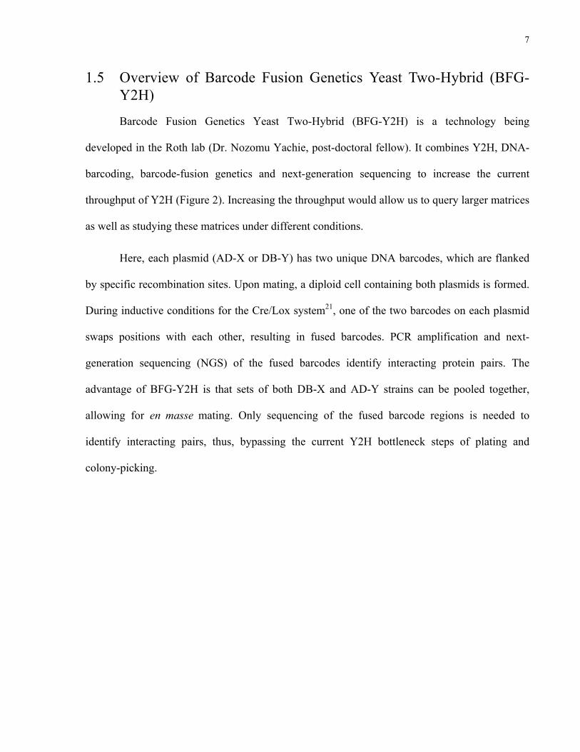
Barcode Fusion Genetics Yeast Two-Hybrid (BFG-Y2H) is a technology being

developed in the Roth lab (Dr. Nozomu Yachie, post-doctoral fellow). It combines Y2H, DNA-

barcoding, barcode-fusion genetics and next-generation sequencing to increase the current

throughput of Y2H (Figure 2). Increasing the throughput would allow us to query larger matrices

as well as studying these matrices under different conditions.

Here, each plasmid (AD-X or DB-Y) has two unique DNA barcodes, which are flanked

by specific recombination sites. Upon mating, a diploid cell containing both plasmids is formed.

During inductive conditions for the Cre/Lox system21, one of the two barcodes on each plasmid

swaps positions with each other, resulting in fused barcodes. PCR amplification and next-

generation sequencing (NGS) of the fused barcodes identify interacting protein pairs. The

advantage of BFG-Y2H is that sets of both DB-X and AD-Y strains can be pooled together,

allowing for en masse mating. Only sequencing of the fused barcode regions is needed to

identify interacting pairs, thus, bypassing the current Y2H bottleneck steps of plating and

colony-picking.

8

Figure 2. Barcode Fusion Genetics Y2H (BFG-Y2H). BFG-Y2H combines Y2H, DNA-

barcoding, barcode-fusion genetics (BFG) and next-generation sequencing (NGS) to increase the

current throughput of Y2H. Here, each plasmid (AD-X/DB-Y) has two unique DNA barcodes

(either the DB TAGs or the AD TAGs in the figure); upon mating and inductive conditions for

the Cre/Lox system, one of the two barcodes on each plasmid swaps positions with each other

within the diploid cell (shown by dotted lines), producing fused barcodes. PCR amplification and

next-generation sequencing of the fused barcodes identify interacting protein pairs. Image

modified from Yachie et al. (unpublished).

9

1.6 BFG-Y2H helps to uncover novel interactions amongst DNA damage repair proteins

In this study, we applied BFG-Y2H to capture PPIs amongst 263 selected yeast DNA

damage repair proteins. DNA damage repair proteins are of particular interest because they

preserve genome integrity in all organisms22. If left unrepaired, DNA damage can have

deleterious effects because it can result in mutations and chromosomal aberrations. Defects in

DNA damage are known to cause increased cancer risks, developmental defects and

neurodegenerative diseases23. Moreover, DNA damage repair proteins are nuclear, making them

a great choice to use in BFG-Y2H.

I found novel Y2H interactions with BFG-Y2H. I confirmed five of these interactions to

be novel when checked against literature. Additionally, I determined which positive controls

should be used in the BFG-Y2H screens and I also demonstrated that the BFG-Y2H screens are

highly reproducible.

10

Materials and Methods 2

2.1 Barcode-Fusion Genetics: background strains

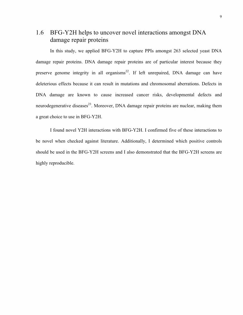
Background strains, RY1010 (MAT a) and RY1030 (MAT alpha), were generated by Dr.

N. Yachie (post-doctoral fellow, Roth lab). Each plasmid contains two unique barcodes

(UPTAG and DNTAG), placed in tandem with loxP and lox2272 sites. The Cre recombinase is

controlled by the Tet-On system24 in our background strains (Figure 3). In the presence of

doxycycline, Cre is able to bind to the rtTA transcription factor and together, they are able to

bind DNA at the tetO2 promoter, allowing the transcription of Cre (Figure 3). The Cre

recombinase allows the barcodes from the AD-X and DB-Y plasmids to switch positions,

generating UPTAG-UPTAG and DNTAG-DNTAG barcode fusions. RY1010 and RY1030 are

derived from Y8800 and Y8930, respectively. Y8800 and Y8930 are generated from Charlie

Boone’s lab by adding cycloheximide resistance to strains generated by James et al.25(see Table

1 for genotypes).

11

Figure 3. Activation of Cre recombinase in our background Y2H strains. A) rtTA and Cre

are integrated into the genomes of the MATa (RY1010) and MATα (RY1030) strains,

respectively. B) In the presence of doxycycline, rtTA is able to bind to the tetO2 promoter and

activate the transcription of Cre recombinase in the diploid yeast cell.

a)

CrePtetO2

rtTAPCMV

rtTA

rtTA

dox

dox

b)

rtTAPCMV CrePtetO2

MAT a MAT α

12

Strain Genotype

Y8800 MATa leu2-3,112 trp1-901 his3-200 ade2-101 ura3-52 gal4Δ gal80Δ cyh2R

LYS2::PGAL1-HIS3 PGAL2-ADE2 MET2::PGAL7-lacZ

Y8930 MATα leu2-3,112 trp1-901 his3-200 ade2-101 ura3-52 gal4Δ gal80Δ cyh2R

LYS2::PGAL1-HIS3 PGAL2-ADE2 MET2::PGAL7-lacZ

RY1010 MATa leu2-3,112 trp1-901 his3-200 ade2-101 ura3-52 gal4Δ gal80Δ cyh2R

LYS2::PGAL1-HIS3 PGAL2-ADE2 MET2::PGAL7-lacZ

can1Δ::PCMV-rtTA-KanMX4

RY1030 MATα leu2-3,112 trp1-901 his3-200 ade2-101 ura3-52 gal4Δ gal80Δ cyh2R

LYS2::PGAL1-HIS3 PGAL2-ADE2 MET2::PGAL7-lacZ

can1Δ::TADH1-PtetO2-Cre-TCYC1-KanMX4

Table 1. Genotypes for the BFG-Y2H background strains. RY1010 and RY1030 are the

BFG-Y2H background strains, which are derived from strains Y8800 and Y893014, respectively.

13

2.2 Generation of barcoded destination vectors

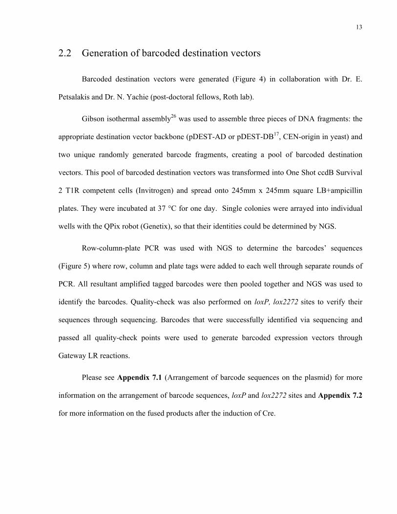
Barcoded destination vectors were generated (Figure 4) in collaboration with Dr. E.

Petsalakis and Dr. N. Yachie (post-doctoral fellows, Roth lab).

Gibson isothermal assembly26 was used to assemble three pieces of DNA fragments: the

appropriate destination vector backbone (pDEST-AD or pDEST-DB17, CEN-origin in yeast) and

two unique randomly generated barcode fragments, creating a pool of barcoded destination

vectors. This pool of barcoded destination vectors was transformed into One Shot ccdB Survival

2 T1R competent cells (Invitrogen) and spread onto 245mm x 245mm square LB+ampicillin

plates. They were incubated at 37 °C for one day. Single colonies were arrayed into individual

wells with the QPix robot (Genetix), so that their identities could be determined by NGS.

Row-column-plate PCR was used with NGS to determine the barcodes’ sequences

(Figure 5) where row, column and plate tags were added to each well through separate rounds of

PCR. All resultant amplified tagged barcodes were then pooled together and NGS was used to

identify the barcodes. Quality-check was also performed on loxP, lox2272 sites to verify their

sequences through sequencing. Barcodes that were successfully identified via sequencing and

passed all quality-check points were used to generate barcoded expression vectors through

Gateway LR reactions.

Please see Appendix 7.1 (Arrangement of barcode sequences on the plasmid) for more

information on the arrangement of barcode sequences, loxP and lox2272 sites and Appendix 7.2

for more information on the fused products after the induction of Cre.

14

Figure 4. Generation of barcoded destination vectors. Two fragments of degenerate

oligonucleotides (NNNN in the figure) and the destination vector’s backbone are used to

generate barcoded destination vectors. This pool of barcoded destination vectors is then

transformed into E. coli cells, spread on large agar plates and single colonies are arrayed into

individual wells. The identity of the barcodes in each well is identified by Row-Column-Plate

PCR (RCP-PCR). Image modified Yachie et al. (unpublished).

15

Figure 5. Row-column-plate PCR (RCP PCR). Row, column and plate tags are added to each

well through separate rounds of PCR. All amplified barcodes are pooled together and NGS is

then used to identify the barcodes. Image modified from Yachie et al. (unpublished).

16

2.3 Selection of DNA damage repair proteins

With the help of Dr. Javier Diaz (post-doctoral fellow, Roth lab), Dr. Atina Cote

(research associate, Roth lab) and Dr. Dan Durocher (PI, Durocher lab), we selected 263 yeast

DNA damage repair proteins from many resources (see Table 2): from Saccharomyces Genome

Database27 annotations (114, “sgd_annotation”), from Alvaro et al.28 due to deletions increasing

the levels of Rad52 foci (69, “rad52_foci”), from REPAIRtoire29, a database with literature

curated proteins that are involved in DNA repair pathways (61, “repairtoire”), manually selected

(84, “core”), from FuncBase30 predictions (6, “yeast_func”) made by using GO terms from the

“core” set and DNA damage repair proteins from the top 5 centroid genes from each of the 50

clusters in Costanzo et al.31 (21, “survey”). Some genes fall under multiple categories, please see

Table 2 for a complete list of genes.

17

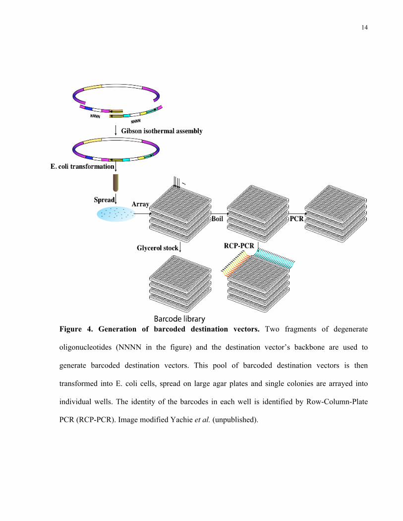
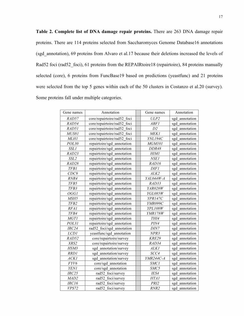
Table 2. Complete list of DNA damage repair proteins. There are 263 DNA damage repair

proteins. There are 114 proteins selected from Saccharomyces Genome Database16 annotations

(sgd_annotation), 69 proteins from Alvaro et al.17 because their deletions increased the levels of

Rad52 foci (rad52_foci), 61 proteins from the REPAIRtoire18 (repairtoire), 84 proteins manually

selected (core), 6 proteins from FuncBase19 based on predictions (yeastfunc) and 21 proteins

were selected from the top 5 genes within each of the 50 clusters in Costanzo et al.20 (survey).

Some proteins fall under multiple categories.

Gene names Annotation Gene names Annotation RAD57 core/repairtoire/rad52_foci ULP2 sgd_annotation RAD54 core/repairtoire/rad52_foci ABF1 sgd_annotation RAD51 core/repairtoire/rad52_foci D2 sgd_annotation MUS81 core/repairtoire/rad52_foci MEK1 sgd_annotation MLH1 core/repairtoire/rad52_foci YNL194C sgd_annotation POL30 repairtoire/sgd_annotation MGM101 sgd_annotation SSL1 repairtoire/sgd_annotation DDR48 sgd_annotation

RAD23 repairtoire/sgd_annotation HIM1 sgd_annotation SSL2 repairtoire/sgd_annotation NSE1 sgd_annotation

RAD28 repairtoire/sgd_annotation RAD16 sgd_annotation TFB1 repairtoire/sgd_annotation DIF1 sgd_annotation CDC9 repairtoire/sgd_annotation ALK2 sgd_annotation RNR4 repairtoire/sgd_annotation YAL044W-A sgd_annotation TFB5 repairtoire/sgd_annotation RAD33 sgd_annotation TFB3 repairtoire/sgd_annotation YAR028W sgd_annotation OGG1 repairtoire/sgd_annotation YGL085W sgd_annotation MSH5 repairtoire/sgd_annotation YPR147C sgd_annotation TFB2 repairtoire/sgd_annotation YMR099C sgd_annotation RFA1 repairtoire/sgd_annotation YPL108W sgd_annotation TFB4 repairtoire/sgd_annotation YMR178W sgd_annotation MGT1 repairtoire/sgd_annotation THI4 sgd_annotation POL31 repairtoire/sgd_annotation PIN4 sgd_annotation IRC24 rad52_foci/sgd_annotation DIN7 sgd_annotation LCD1 yeastfunc/sgd_annotation NPR3 sgd_annotation

RAD52 core/repairtoire/survey KRE29 sgd_annotation XRS2 core/repairtoire/survey RAD34 sgd_annotation HSM3 sgd_annotation/survey ALK1 sgd_annotation RRD1 sgd_annotation/survey SCC4 sgd_annotation ACK1 sgd_annotation/survey YMR244C-A sgd_annotation FYV6 core/sgd_annotation SMC1 sgd_annotation YEN1 core/sgd_annotation SMC5 sgd_annotation IRC25 rad52_foci/survey IES4 sgd_annotation MAD2 rad52_foci/survey HTA1 sgd_annotation IRC16 rad52_foci/survey PRI2 sgd_annotation VPS72 rad52_foci/survey RNR2 sgd_annotation

18

MAD1 rad52_foci/survey SMC6 sgd_annotation NUP133 rad52_foci/survey NSE5 sgd_annotation VPS71 rad52_foci/survey PAN3 sgd_annotation CTF19 rad52_foci/survey YPR022C sgd_annotation IRC21 rad52_foci/survey YHR192W sgd_annotation YKU70 core/repairtoire MND1 sgd_annotation UNG1 core/repairtoire PPH3 extra_manual MAG1 core/repairtoire CHL1 extra_manual APN2 core/repairtoire MMS4 core/survey LIF1 core/repairtoire SWC5 core/survey RAD2 core/repairtoire RAD17 core/survey RAD1 core/repairtoire SRS2 core/survey

RAD50 core/repairtoire MRC1 core/survey NTG2 core/repairtoire RAD61 core/survey

RAD30 core/repairtoire SEM1 repairtoire MSH6 core/repairtoire DPB4 repairtoire POL4 core/repairtoire SPO11 repairtoire

MRE11 core/repairtoire RFC5 repairtoire REV3 core/repairtoire DPB2 repairtoire PHR1 core/repairtoire DPB3 repairtoire

RAD10 core/repairtoire HNT3 repairtoire RAD27 core/repairtoire CCL1 repairtoire MSH2 core/repairtoire MRPL1 rad52_foci MSH4 core/repairtoire RTT103 rad52_foci MEC1 core/repairtoire IRC19 rad52_foci MPH1 core/repairtoire COX16 rad52_foci EXO1 core/repairtoire IRC18 rad52_foci PSO2 core/repairtoire PAC10 rad52_foci TDP1 core/repairtoire CBT1 rad52_foci MSH3 core/repairtoire IRC23 rad52_foci DNL4 core/repairtoire MDM20 rad52_foci RAD3 core/repairtoire IRC22 rad52_foci POL32 core/repairtoire IRC4 rad52_foci NEJ1 core/repairtoire IRC7 rad52_foci PBY1 yeastfunc/survey DAK2 rad52_foci

RAD59 core/rad52_foci RIM9 rad52_foci SLX8 core/rad52_foci NUP60 rad52_foci ESC2 core/rad52_foci GSH2 rad52_foci

RTT109 core/rad52_foci ATR1 rad52_foci RMI1 core/rad52_foci HST3 rad52_foci MMS1 core/rad52_foci PAP2 rad52_foci

RTT107 core/rad52_foci TOF2 rad52_foci RTT101 core/rad52_foci BDF1 rad52_foci

SAE2 core/rad52_foci ECM11 rad52_foci WSS1 core/rad52_foci BUB2 rad52_foci RRM3 core/rad52_foci HPR1 rad52_foci

YKR075C sgd_annotation YMR027W rad52_foci YLR118C sgd_annotation IRC3 rad52_foci YLR271W sgd_annotation IRC8 rad52_foci

HUG1 sgd_annotation IZH2 rad52_foci SML1 sgd_annotation IRC15 rad52_foci

ADD37 sgd_annotation SGO1 rad52_foci

19

TPP1 sgd_annotation LAG2 rad52_foci YDR262W sgd_annotation BUD27 rad52_foci

NSE3 sgd_annotation GDH1 rad52_foci HHO1 sgd_annotation IRC10 rad52_foci RCN2 sgd_annotation MRP17 rad52_foci

YNL134C sgd_annotation AHC1 rad52_foci YJR085C sgd_annotation RCO1 rad52_foci YJR011C sgd_annotation MED1 rad52_foci

HAT1 sgd_annotation DDR2 rad52_foci IES6 sgd_annotation MAD3 rad52_foci

YJL144W sgd_annotation MRPS16 rad52_foci LSM12 sgd_annotation IRC6 rad52_foci

YML131W sgd_annotation YMR31 rad52_foci YJR096W sgd_annotation PSY4 yeastfunc YGR126W sgd_annotation YDL156W yeastfunc

HHT1 sgd_annotation PSY2 yeastfunc YHL018W sgd_annotation HDA1 yeastfunc

YIM1 sgd_annotation SHU2 core MMS21 sgd_annotation ASF1 core

YFR017C sgd_annotation CSM3 core RFA3 sgd_annotation MGS1 core

YDL119C sgd_annotation PSY3 core DDI3 sgd_annotation SLX4 core HHT2 sgd_annotation SAW1 core HTA2 sgd_annotation CHK1 core DDI1 sgd_annotation RAD55 core

CRT10 sgd_annotation RPN4 core YBL036C sgd_annotation CLA4 core

PRI1 sgd_annotation DOA1 core RAD53 sgd_annotation PIF1 core DDI2 sgd_annotation NFI1 core MIG3 sgd_annotation CTF18 core ECO1 sgd_annotation MSH1 core BER1 sgd_annotation CSM2 core RNR3 sgd_annotation SLX1 core RAD7 sgd_annotation SIZ1 core

HRR25 sgd_annotation RDH54 core LDB16 sgd_annotation REV1 core RPH1 sgd_annotation RAD9 core RNR1 sgd_annotation MEC3 core

FMP41 sgd_annotation MLH2 core YOR062C sgd_annotation DCC1 core

OCA1 sgd_annotation SLX5 core ULP2 sgd_annotation RAD6 core ABF1 sgd_annotation RAD5 core

D2 sgd_annotation TOP3 core

20

2.4 Generating barcoded Y2H strains

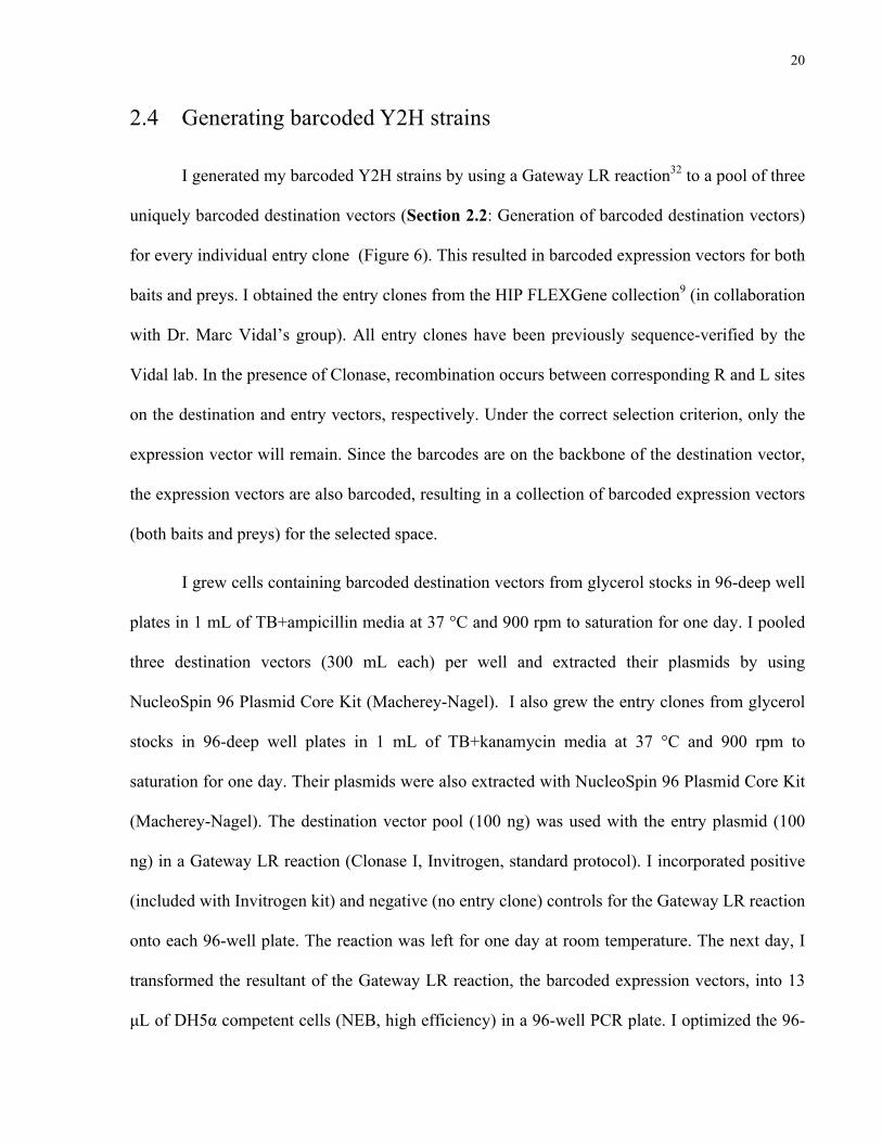
I generated my barcoded Y2H strains by using a Gateway LR reaction32 to a pool of three

uniquely barcoded destination vectors (Section 2.2: Generation of barcoded destination vectors)

for every individual entry clone (Figure 6). This resulted in barcoded expression vectors for both

baits and preys. I obtained the entry clones from the HIP FLEXGene collection9 (in collaboration

with Dr. Marc Vidal’s group). All entry clones have been previously sequence-verified by the

Vidal lab. In the presence of Clonase, recombination occurs between corresponding R and L sites

on the destination and entry vectors, respectively. Under the correct selection criterion, only the

expression vector will remain. Since the barcodes are on the backbone of the destination vector,

the expression vectors are also barcoded, resulting in a collection of barcoded expression vectors

(both baits and preys) for the selected space.

I grew cells containing barcoded destination vectors from glycerol stocks in 96-deep well

plates in 1 mL of TB+ampicillin media at 37 °C and 900 rpm to saturation for one day. I pooled

three destination vectors (300 mL each) per well and extracted their plasmids by using

NucleoSpin 96 Plasmid Core Kit (Macherey-Nagel). I also grew the entry clones from glycerol

stocks in 96-deep well plates in 1 mL of TB+kanamycin media at 37 °C and 900 rpm to

saturation for one day. Their plasmids were also extracted with NucleoSpin 96 Plasmid Core Kit

(Macherey-Nagel). The destination vector pool (100 ng) was used with the entry plasmid (100

ng) in a Gateway LR reaction (Clonase I, Invitrogen, standard protocol). I incorporated positive

(included with Invitrogen kit) and negative (no entry clone) controls for the Gateway LR reaction

onto each 96-well plate. The reaction was left for one day at room temperature. The next day, I

transformed the resultant of the Gateway LR reaction, the barcoded expression vectors, into 13

µL of DH5α competent cells (NEB, high efficiency) in a 96-well PCR plate. I optimized the 96-

21

well Gateway LR reactions such that at least 95% of the E. coli transformants have more than 10

colonies per 5 µL of spotted transformed cells. I assessed each experiment’s cloning and

transformation efficiencies by spotting 5 µL of the transformed cells onto LB+ampicillin

OmniTrays. In parallel, I grew the rest of the transformed E. coli cells for one day in 96-deep

well plates containing 1 mL of LB+ampicillin. I extracted the plasmids the following day with

NucleoSpin 96 Plasmid Core Kit (Macherey-Nagel). I spot-checked the resultant expression

clones on each plate with NGS to ensure correct plate orientations. I transformed these plasmids

into the appropriate yeast background strains (RY1010 for the AD/preys or RY1030 for

DB/baits) by using Frozen-EZ Yeast Transformation II Kit (Zymo Research).

Because generating barcoded Y2H strains is one of the most time-consuming and costly

steps of BFG-Y2H, I attempted to develop a more high-throughput method by using an en masse

Gateway LR reaction to increase the efficiency of generating barcoded Y2H strains. Please see

Appendix 7.3 (Using an en masse Gateway LR reaction to generate barcoded strains) for more

details.

22

Figure 6. Gateway LR reaction between a barcoded destination vector and an entry clone.

The destination vector (pDEST-DB) is barcoded (NNN) and flanked by corresponding loxP

sites. In the presence of Clonase®, recombination occurs between corresponding R and L sites

on the destination and entry vectors, respectively, and generates an expression product (pEXP-

DB) that is barcoded and a by-product. Due to selection criterion, out of all four vectors, only the

barcoded expression vector will remain.

23

2.5 BFG-Y2H screens

The BFG-Y2H screening procedure was developed and optimized by Dr. N. Yachie

(Roth lab). It took me 10 days to complete the screen up to the generation of the sequencing

libraries to identify the fused barcodes. A complete BFG-Y2H screen contains three conditions:

with histidine (+His), without histidine (-His) and with 3-amino-1,2,4-triazole (+3AT). The +His

condition is the non-selective condition, which gives us an estimate of the complexity of the

screen with regard to diploid cells before being subjected to selection conditions. The –His

condition is the selective condition for interacting protein pairs. The +3AT condition is a more

stringent selective condition for interacting protein pairs, as 3AT is a competitive inhibitor of the

HIS3 gene product34.

I grew cells with barcoded expression vectors from glycerol stocks in 96-deep well plates

containing 1mL of SC-Leu+Ade or SC-Trp+Ade media for the DB-X and AD-Y pools,

respectively. The deep well plates were grown at 30 °C and 900 rpm to saturation for two days. I

pooled the DB-X and AD-Y pools separately, at equal cell densities (700 OD600nm units of each)

and washed twice with water. I then resuspended the cells in water and pooled them together at

equal OD600nm units. The cells were left for 3 hours at room temperature to increase mating

efficiency35. I pelleted cells and removed the supernatant, and I spread the remaining cell pellets

directly onto YPAD plates (technical replicates) and the plates were incubated for one day at

room temperature. The next day, I scraped the cells off the plates and collected them with water.

I washed the cells twice with water and I resuspended them in 500mLs of SC-Leu-Trp+His+Ade

media in a 2L flask to a final 1.0 OD600nm/mL. The cells were incubated for two days at 30 °C

and 200 rpm to enrich for diploid cells. Afterwards, I washed the diploid cells with water and

resuspended in water. I spread 200uL of cells at a density of 1.0 OD600nm/mL (108 diploid cells)

24

onto 150mm agar plates. The plates were non-selective condition (“+His”, SC-Leu-

Trp+His+Ade and selective conditions (“-His”, SC-Leu-Trp-His+Ade and “+3AT”, SC-Leu-Trp-

His+Ade+3AT at 1mM amino-1,2,4-triazole).

After 3 days of incubating the selection plates at 30 °C, I scraped the cells from the plates

and washed them twice with water. I resuspended the cells in 5mL SC-Leu-

Trp+His+Ade+Doxycycline (10µg/mL) at a final concentration of 1.0 OD600nm/mL. The cells

were incubated over night at 30 °C and 200 rpm for the induction of Cre. The following day, I

extracted the plasmid DNA from 3 OD600nm units of cells by using Charge Switch Plasmid Yeast

Mini Kit (Invitrogen). Fused barcodes were amplified with primers carrying Illumina paired-end

multiplexed sequencing primers. The amplified products were size-selected by E-Gel SizeSelect

2% Agarose gel (Invitrogen) and they were sequenced on the HiSeq2500 (Illumina). The barcode

reads were mapped with Bowtie236.

25

2.6 Replicates for the BFG-Y2H screens

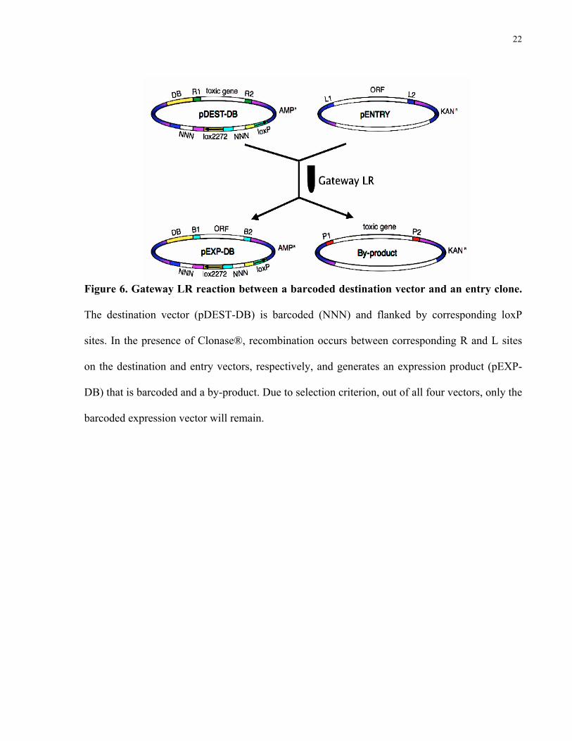
There are several ways to assess the reproducibility of BFG-Y2H screens (Figure 7)

Firstly, I performed two screen replicates of the BFG-Y2H screen, which were separated at the

mating stage and onwards (Figure 7, panel A). Secondly, I implemented another level of

replicates at the barcoded strain level, where I created two to three different expression clones for

each ORF, each represented by a different barcode. Upon mating, the resulting diploid cell will

contain different combinations of the barcodes (Figure 7, panel B), and I consider these to be

biological replicates. Lastly, there are two sets of fused barcodes within each diploid cell, UP-UP

and DN-DN (Figure 7, panel C). Please see Figure 8 for the visualization of the relative

positions of each type of replicate within the BFG-Y2H screen.

26

Figure 7. Assessing the reproducibility of BFG-Y2H. There are three levels of replication that

I implemented during the BFG-Y2H screen. A) Screen replicates that were separated from the

mating phase and onwards. B) Biological strain replicates: two to three uniquely barcoded strains

for each ORF were used to mate together to generate different combinations of diploid cells. In

this example, the bait and prey are represented by two different barcodes, resulting in four

different combinations of the diploid cells after mating. C) Internal replicates: two pairs of fused

barcodes (UP-UP and DN-DN) are within each diploid cell, serving as another way of assessing

reproducibility

UpUp fusionDnDn fusion

X

A) Screen replicates B) Biological strain replicates

DB-X AD-Y

C) Internal replicates

27

Figure 8. Replicates within the BFG-Y2H screen. Visual representation of the different kind

of replicates within the BFG-Y2H screen: A) screen replicates have been separated at the mating

stage, B) biological strain replicates are different diploids generated from differently barcoded

haploid strains C) internal replicates of the UP-UP and DN-DN fusion barcodes within each

diploid cell.

28

2.7 Pairwise retesting

I performed pairwise retesting for candidate interactions from the BFG-Y2H screens by

following the protocol mentioned in Rual et al.37 with slight modifications as follows. Four

experimental repeats were performed of the mating stage and onwards.

I used AD-null cells as negative controls to determine auto-activators in the pairwise

retesting experiment. The AD-null expression vectors don’t have an ORF inserted (obtained

from the Vidal lab). These plasmids were then transformed into RY1010. I also selected 3 pairs

of previously known positive Y2H interactions as positive controls (obtained from the Vidal lab).

I grew barcoded Y2H strains from glycerol stocks in 96-well culture plates containing

150µL of SC-Leu+Ade or SC-Trp+Ade media for DB-X and AD-Y strains, respectively. The

cells were grown at 30 °C at 900rpm for one day to saturation. The next day, I mated the

corresponding DB-X and AD-Y cells by combining them at equal volumes (100µL:100µL). I

resuspended the cells in 100µL of YPAD and repelleted them. The cells were left at room

temperature for one day. In parallel, I also mated all DB-X cells with AD-null cells.

The following day, I washed the cells twice with water and resuspended them in 100µL

of diploid selection media (SC-Leu-Trp+His+Ade). I enriched for diploid cells by taking 10µL of

these mated samples to grow in 96-deep well plates containing 1mL of diploid selection media.

The cells were incubated at 30 °C at 900rpm for two days. I washed the cells with 100µL of

water twice, and resuspended the cells in 100µL of water. I diluted the cells by 100-fold, and

spotted 5µL of the diluted cells onto different selection plates (+His, -His, +3AT). The plates

were incubated at 30 °C for two days.

29

2.8 Calculation of interaction scores

For each screen, interaction scores (∆𝑠) are calculated. The calculation can be divided

into two steps: (1) the normalization of barcode counts and (2) distinguishing the real positive

interactions from autoactivators. This calculation scheme was developed by Dr. N. Yachie and

the implementation was carried out with help from Dr. E. Petsalakis.

The normalization of barcodes was done using the non-selective condition (+His). This is

because not all protein pairs are equally represented. Some causes of this are due to, but not

limited to, some ORFs’ barcodes are missing due to failed cloning, toxicity effects of the ORF in

the nucleus and some barcodes may not sequence as well due to inherent sequence biases.

Let 𝑐!!" represent the barcode counts of the protein pair 𝐷𝐵! and 𝐴𝐷! in the non-selective

condition (+His). Let 𝑓!i be the marginal frequency of all barcodes containing DBi, which is an

entire row of the matrix:

𝑓!! =  𝑐!!,!!

!!!

𝑡𝑜𝑡𝑎𝑙!

Where 𝑗 represents the row number and 𝑡𝑜𝑡𝑎𝑙!is the total count of the barcodes in the non-

selective condition (+His). The frequency of the protein pair 𝐴𝐷! and 𝐷𝐵! in the +His condition

is represented by 𝑓!!":

𝑓!!" = 𝑓!!×  𝑓!!

This is used instead of the raw barcode counts due to limited sequencing coverage across the

entire matrix and sample complexity. For the selective conditions (-His or +3AT), the marginal

frequency of the protein pair 𝐴𝐷! and 𝐷𝐵! is 𝑓!!":

30

𝑓!!" =𝑐!!" +  𝛼𝑡𝑜𝑡𝑎𝑙!

The sequencing coverage for selection conditions is much better, and for those strains that

survive, the raw barcode counts (𝑐!!") could be used to calculate the frequencies of each

individual protein pair. 𝛼  was set to 1 to avoid having 0 values for 𝑓!!".

The enrichment of the positive protein interactions in the selective condition is shown

with 𝑠!":

𝑠!" =𝑓!!"𝑓!!"

Background autoactivators are eliminated by adjusting the 𝑠!" scores:

If 𝑠!" − 𝑠! ≥  𝛽! , then ∆𝑠!" =!!"!!!!!

If 𝑠!" − 𝑠! <  𝛽! , then ∆𝑠!" = 1

Where 𝑠! is the median value of all 𝑠! and 𝛽! is the 75th percentile value of the positive

distribution of 𝑠!" − 𝑠!. This effectively eliminates the autoactivators by taking only the top 1/8th

(12.5%) of the 𝑠! scores.

2.9 Statistical analysis and datasets used

I used R (version 3.1.0) to calculate Pearson’s correlation coefficients with the ‘stats’

package (included in base library). I visualized interactomes with Cytoscape38 (version 2.8.0). I

used datasets from BioGRID (Saccharomyces cerevisiae v2.0.63).

31

Results 3

3.1 Reproducibility of the BFG-Y2H screens

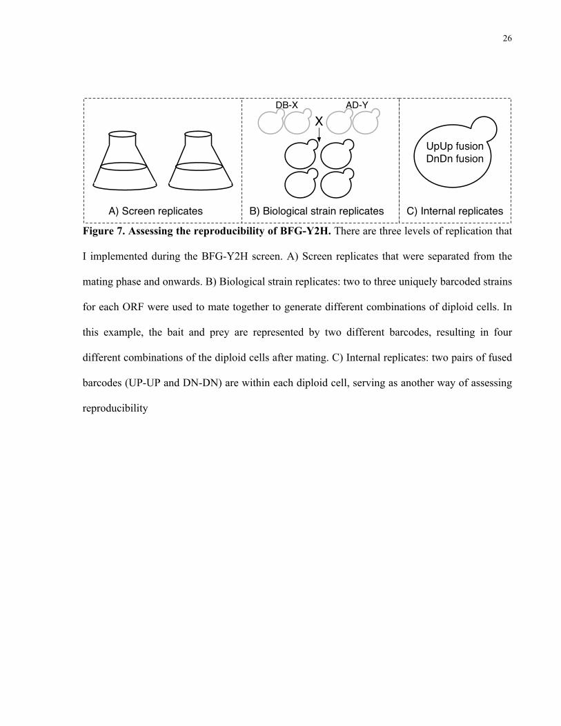
The reproducibility of the internal replicates (two sets of barcodes within each diploid

cell, Figure 7 panel C) is shown by several correlation plots (Figure 9 a-c), where the raw read

counts (Up-Up fusion and Dn-Dn fusion) of fused barcodes have been transformed to a log scale.

Pearson’s correlation coefficients (PCC) were calculated with the raw read counts (all p-values

were < 2.2e-16). The correlation value for the +His condition (0.72) is lower than the selective

conditions (0.95 and 0.89 for –His and +3AT, respectively).

The +His population was used only to determine the marginal frequencies of the input

barcodes; therefore, it was not necessary to obtain coverage of each individual barcode pair.

32

Figure 9. Reproducibility of BFG-Y2H between two internal replicates. Correlation plots for

both non-selective (a) and selective conditions (b and c). The axes represent the raw read counts

in log scale. The correlation is performed between the raw barcode counts. Pearson’s correlation

coefficients (PCC) are shown (all p-values were < 2.2e-16).

PCC=  0.72  

a)

PCC=  0.95  

b)

PCC=  0.89  

c)

33

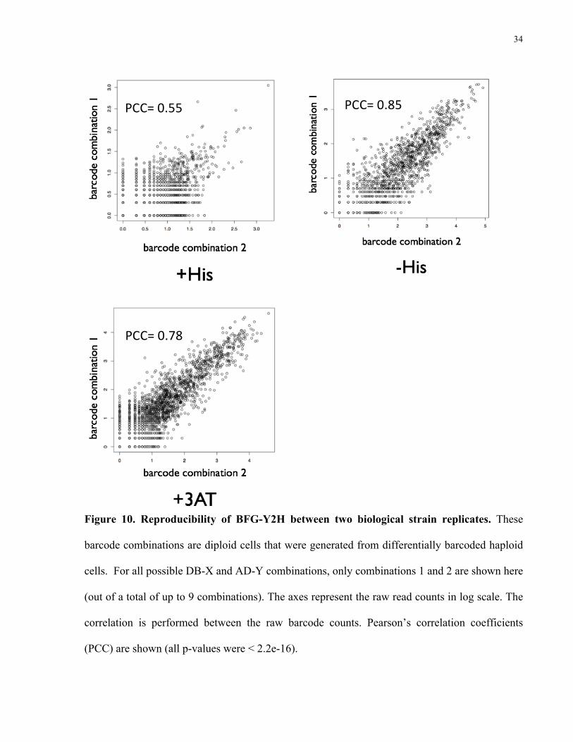
Reproducibility between biological strain replicates (barcode strain combinations, recall

Figure 7 panel B) is shown in Figure 10 a-c. Similarly, the raw read counts of fused barcodes

have been transformed to a log scale. PCCs were calculated with the raw read counts (all p-

values were <2.2e16). The correlation value for the +His condition (0.55) is lower than the

selective conditions (0.85 and 0.78 for –His and +3AT, respectively). There are fewer data

points on these scatter plots because they only contain counts for barcode combination 1 and

barcode combination 2 of replicate 1, whereas the previous plots contain all the unique barcode

combinations.

34

Figure 10. Reproducibility of BFG-Y2H between two biological strain replicates. These

barcode combinations are diploid cells that were generated from differentially barcoded haploid

cells. For all possible DB-X and AD-Y combinations, only combinations 1 and 2 are shown here

(out of a total of up to 9 combinations). The axes represent the raw read counts in log scale. The

correlation is performed between the raw barcode counts. Pearson’s correlation coefficients

(PCC) are shown (all p-values were < 2.2e-16).

PCC=  0.55   PCC=  0.85  

PCC=  0.78  

35

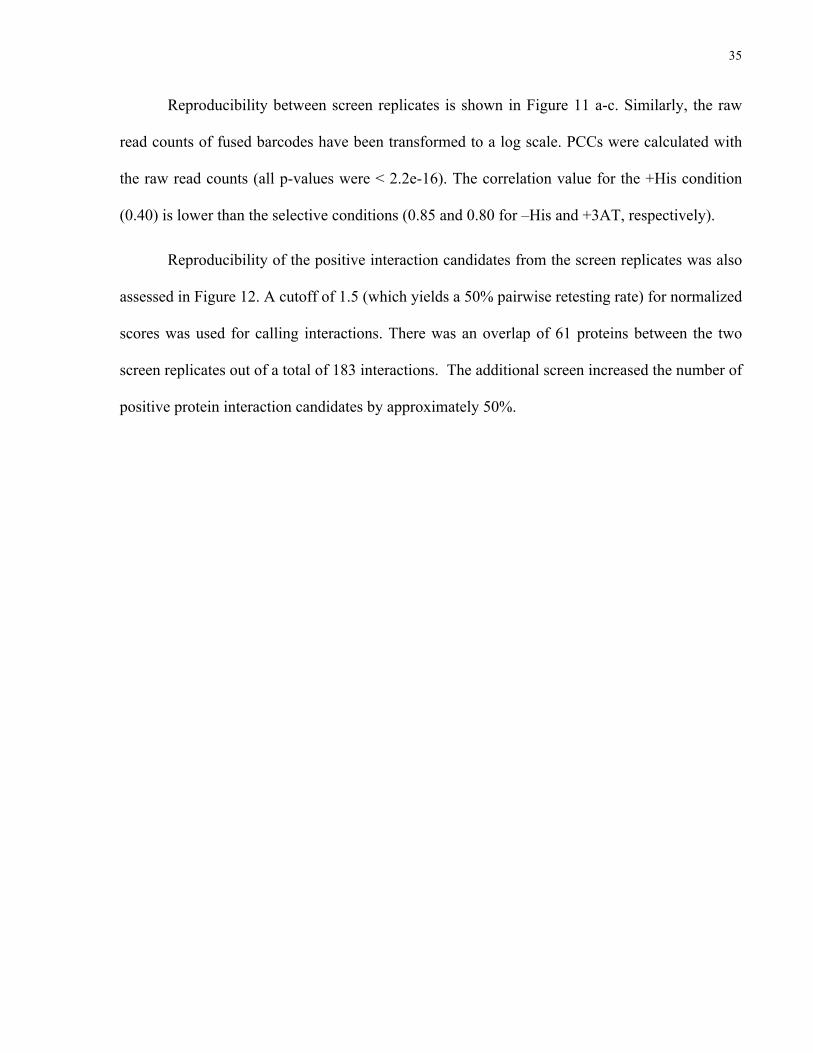
Reproducibility between screen replicates is shown in Figure 11 a-c. Similarly, the raw

read counts of fused barcodes have been transformed to a log scale. PCCs were calculated with

the raw read counts (all p-values were < 2.2e-16). The correlation value for the +His condition

(0.40) is lower than the selective conditions (0.85 and 0.80 for –His and +3AT, respectively).

Reproducibility of the positive interaction candidates from the screen replicates was also

assessed in Figure 12. A cutoff of 1.5 (which yields a 50% pairwise retesting rate) for normalized

scores was used for calling interactions. There was an overlap of 61 proteins between the two

screen replicates out of a total of 183 interactions. The additional screen increased the number of

positive protein interaction candidates by approximately 50%.

36

Figure 11. Reproducibility of BFG-Y2H between two screen replicates. Replicate 1 and 2

have been separated before the mating stage and onwards. The axes represent the raw read

counts in log scale. The correlation is performed between the raw barcode counts. Pearson’s

correlation coefficients (PCC) are shown (all p-values were < 2.2e-16).

PCC=  0.78   PCC=  0.40   PCC=  0.85  

PCC=  0.80  

37

Figure 12. Reproducibility of BFG-Y2H between two screen replicates. This Venn diagram

shows the overlapping positive interaction candidates between two BFG-Y2H screens. A cutoff

of 1.5 for the normalized score was used to determine positive interaction candidates.

61 6458

Normalized score cutoff: 1.5

38

3.2 Positive controls in the BFG-Y2H screens

I included positive Y2H controls (denoted as “Positive Reference Set” or PRS from

hereon) from the Vidal lab (in collaboration with Dr. Nidhi Sahni, Vidal lab) within my BFG-

Y2H screens. The Vidal lab has previously used pairwise Y2H to test ~70,000 human protein

pairs that were curated by the literature as positive binary interactions. This resulted in a list of

~700 positive Y2H interactions that pairwise retested as positives in the Y2H assay for more

than two times (unpublished data from Dr. Nidhi Sahni, post-doctoral fellow, Vidal lab). In

collaboration with Dr. N. Yachie and Dr. E. Petsalakis (Roth lab), 34 positive Y2H interacting

pairs were randomly selected amongst the list of positive Y2H interacting pairs provided by the

Vidal lab. These 34 positive Y2H interacting pairs were classified into two levels by the Vidal

lab. Level 1 contains interacting pairs are reported as bidirectional by the Vidal lab, meaning

that they are Y2H positives in both DB-X/AD-Y and DB-Y/AD-X configurations. Level 2

interaction pairs are reported as positives only in the DB-X/AD-Y direction. 15 of the 34 positive

interactions were level 1 and 19 were level 2 interactions.

The positives are positioned along the diagonal of the matrices. The ideal results would

be to see the diagonal lit up under selective Y2H conditions (Figure 13). The Vidal lab has not

performed pairwise testing for off-diagonal protein pairs; therefore, this space is less known and

not necessarily negative for Y2H protein interactions.

39

Figure 13. Expected positive interactions for BFG-Y2H. Protein pairing information was

obtained from the Vidal lab. There are a total of 34 expected Y2H positive protein interactions

(black) along the diagonal divided into two levels. Level 1 (15/34) interacting pairs are reported

as bidirectional by the Vidal lab, meaning that they are Y2H positives in both DB-X/AD-Y and

DB-Y/AD-X configurations. Level 2 (19/34) interaction pairs are reported as positives only in

the DB-X/AD-Y direction. The off-diagonal space hasn’t been subjected to pairwise retesting

with Y2H, therefore, this space is unknown and not necessarily negative for Y2H.

40

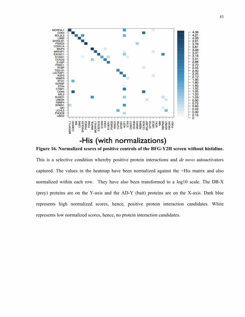
As discussed in section 2.8 (Calculation of interaction scores), the +His condition (Figure

15) serves as a background level to normalize of the barcode counts for both the –His (Figure

16) and +3AT (Figure 17) conditions such that positive interactions can be quantitatively

identified. Spotty sequencing coverage for strains at the +His level is not considered to be

important because marginal frequencies (Section 2.8 Calculation of interaction scores) are used

for downstream normalization (please see Figure 19 for the entire matrix of marginal

frequencies). Figure 15 shows the raw barcode counts for the –His selective condition before

normalizing against the +His matrix and within each row. All values have been transformed to a

log10 scale.

41

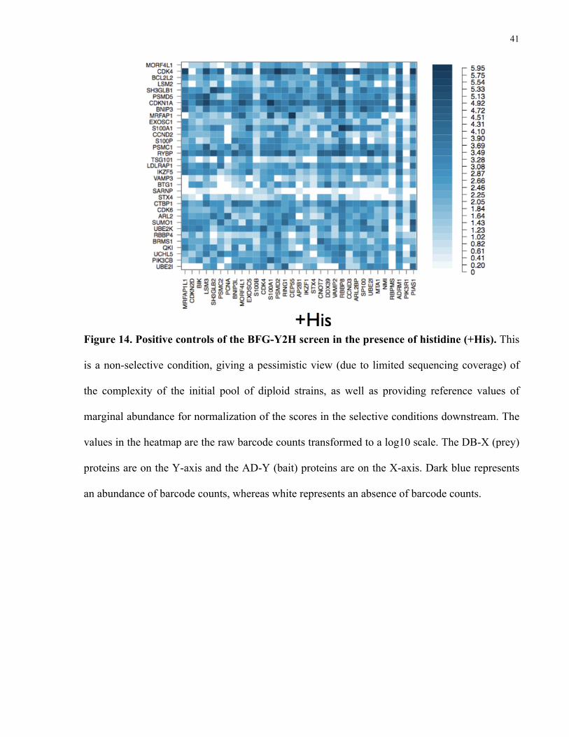
Figure 14. Positive controls of the BFG-Y2H screen in the presence of histidine (+His). This

is a non-selective condition, giving a pessimistic view (due to limited sequencing coverage) of

the complexity of the initial pool of diploid strains, as well as providing reference values of

marginal abundance for normalization of the scores in the selective conditions downstream. The

values in the heatmap are the raw barcode counts transformed to a log10 scale. The DB-X (prey)

proteins are on the Y-axis and the AD-Y (bait) proteins are on the X-axis. Dark blue represents

an abundance of barcode counts, whereas white represents an absence of barcode counts.

42

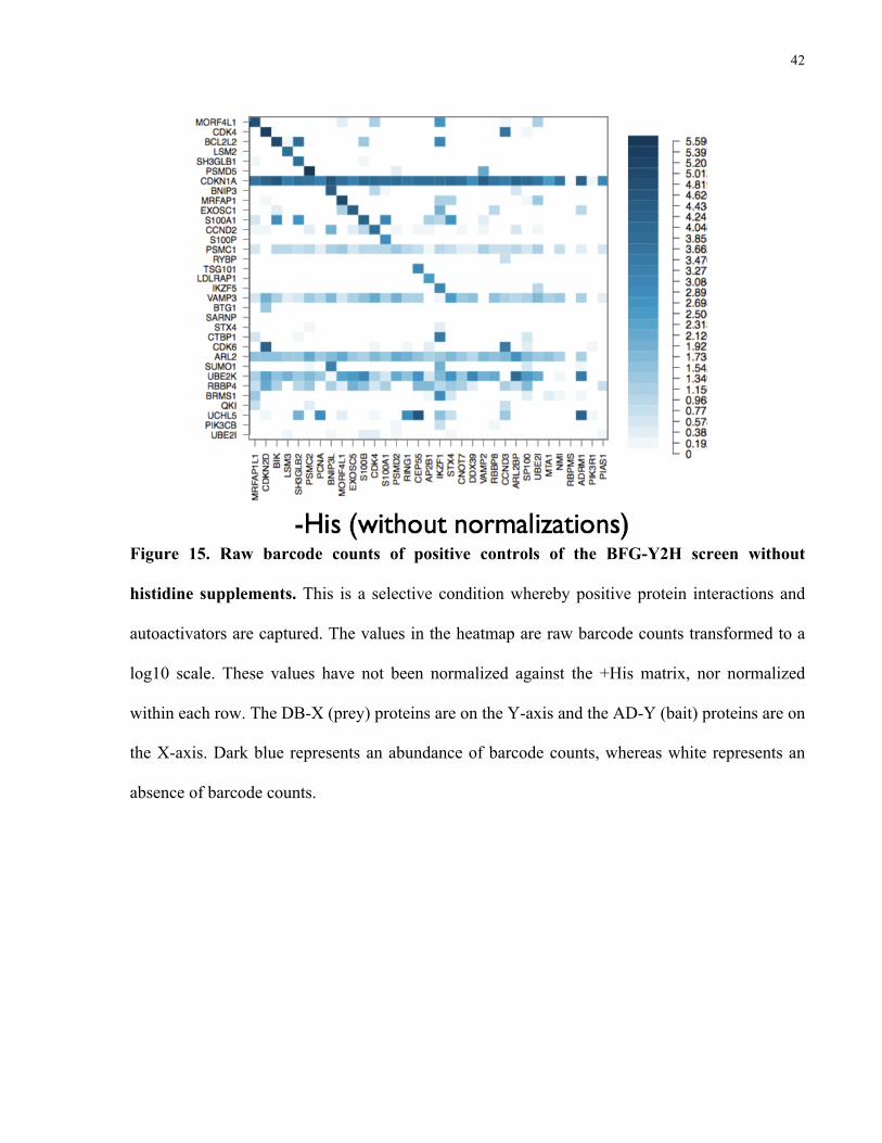
Figure 15. Raw barcode counts of positive controls of the BFG-Y2H screen without

histidine supplements. This is a selective condition whereby positive protein interactions and

autoactivators are captured. The values in the heatmap are raw barcode counts transformed to a

log10 scale. These values have not been normalized against the +His matrix, nor normalized

within each row. The DB-X (prey) proteins are on the Y-axis and the AD-Y (bait) proteins are on

the X-axis. Dark blue represents an abundance of barcode counts, whereas white represents an

absence of barcode counts.

43

Figure 16. Normalized scores of positive controls of the BFG-Y2H screen without histidine.

This is a selective condition whereby positive protein interactions and de novo autoactivators

captured. The values in the heatmap have been normalized against the +His matrix and also

normalized within each row. They have also been transformed to a log10 scale. The DB-X

(prey) proteins are on the Y-axis and the AD-Y (bait) proteins are on the X-axis. Dark blue

represents high normalized scores, hence, positive protein interaction candidates. White

represents low normalized scores, hence, no protein interaction candidates.

44

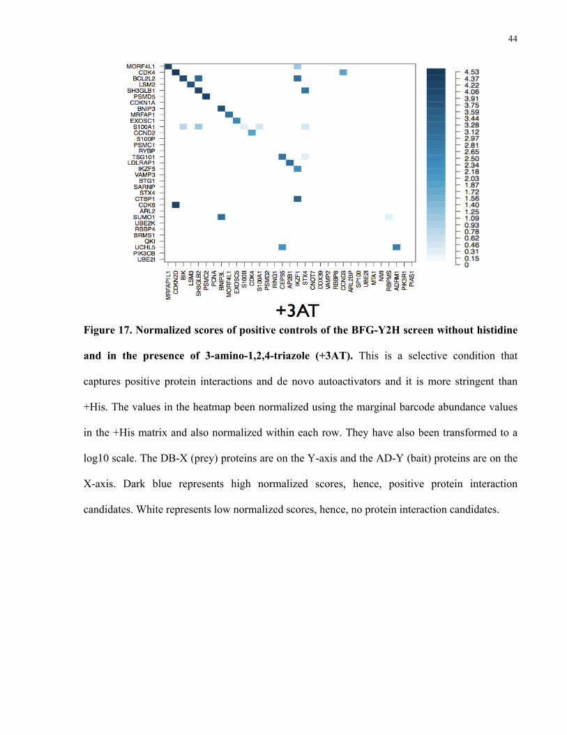
Figure 17. Normalized scores of positive controls of the BFG-Y2H screen without histidine

and in the presence of 3-amino-1,2,4-triazole (+3AT). This is a selective condition that

captures positive protein interactions and de novo autoactivators and it is more stringent than

+His. The values in the heatmap been normalized using the marginal barcode abundance values

in the +His matrix and also normalized within each row. They have also been transformed to a

log10 scale. The DB-X (prey) proteins are on the Y-axis and the AD-Y (bait) proteins are on the

X-axis. Dark blue represents high normalized scores, hence, positive protein interaction

candidates. White represents low normalized scores, hence, no protein interaction candidates.

45

3.3 Untangling positive controls

To address the question of why the BFG-Y2H screens failed to pick up 20 out of 34

(58.8%) of the PRS interactions, I conducted several pairwise-retesting experiments, where each

pair was tested one-on-one per Section 2.7 (Pairwise retesting). A smaller matrix of the original

–His matrix for the positive controls was generated for positive controls that tested positive in

pairwise-retesting in the –His condition (Figure 18), where all protein pairs that tested positive in

the pairwise-retesting experiment are along the diagonal.

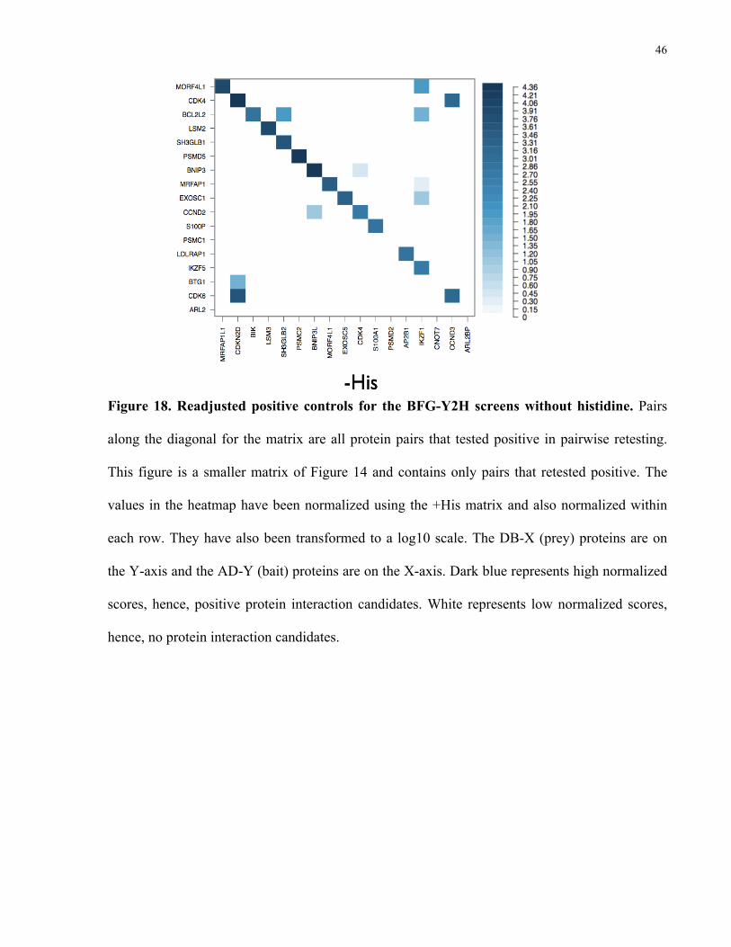
Only 17 protein pairs out of the initial 34 PRS protein pairs retested positive, and three

out of these 17 protein pairs were not detected by the BFG-Y2H screen (PSMC1 and PSMD2,

BTG1 and CNOT7 and ARL2 and ARL2BP). As previously mentioned, the off-diagonal space

has not been pairwise-retested, therefore, positive interactions in this space could be genuine. For

example, the interaction between CDK6 and CDKN2D has been demonstrated through a crystal

structure39. The CDK4 and CCND3 interaction has also been previously shown through Y2H

screens37 as well as affinity capture40,41.

Additional pairwise-retesting experiments were performed to check the effect of different

methods of clone generation on the Y2H results. I compared the pairwise-retesting experimental

results from two different methods of generating clones: Gateway cloning and in-yeast

assembly42 and discovered that Gateway cloning performed better than in-yeast assembly,

however, the two were not statistically different (see Appendix 7.4).

46

Figure 18. Readjusted positive controls for the BFG-Y2H screens without histidine. Pairs

along the diagonal for the matrix are all protein pairs that tested positive in pairwise retesting.

This figure is a smaller matrix of Figure 14 and contains only pairs that retested positive. The

values in the heatmap have been normalized using the +His matrix and also normalized within

each row. They have also been transformed to a log10 scale. The DB-X (prey) proteins are on

the Y-axis and the AD-Y (bait) proteins are on the X-axis. Dark blue represents high normalized

scores, hence, positive protein interaction candidates. White represents low normalized scores,

hence, no protein interaction candidates.

47

3.4 BFG-Y2H screens

In order to uncover novel interactions amongst DNA damage repair proteins, I completed

the BFG-Y2H screens with the DNA damage repair proteins and the PRS in all three conditions:

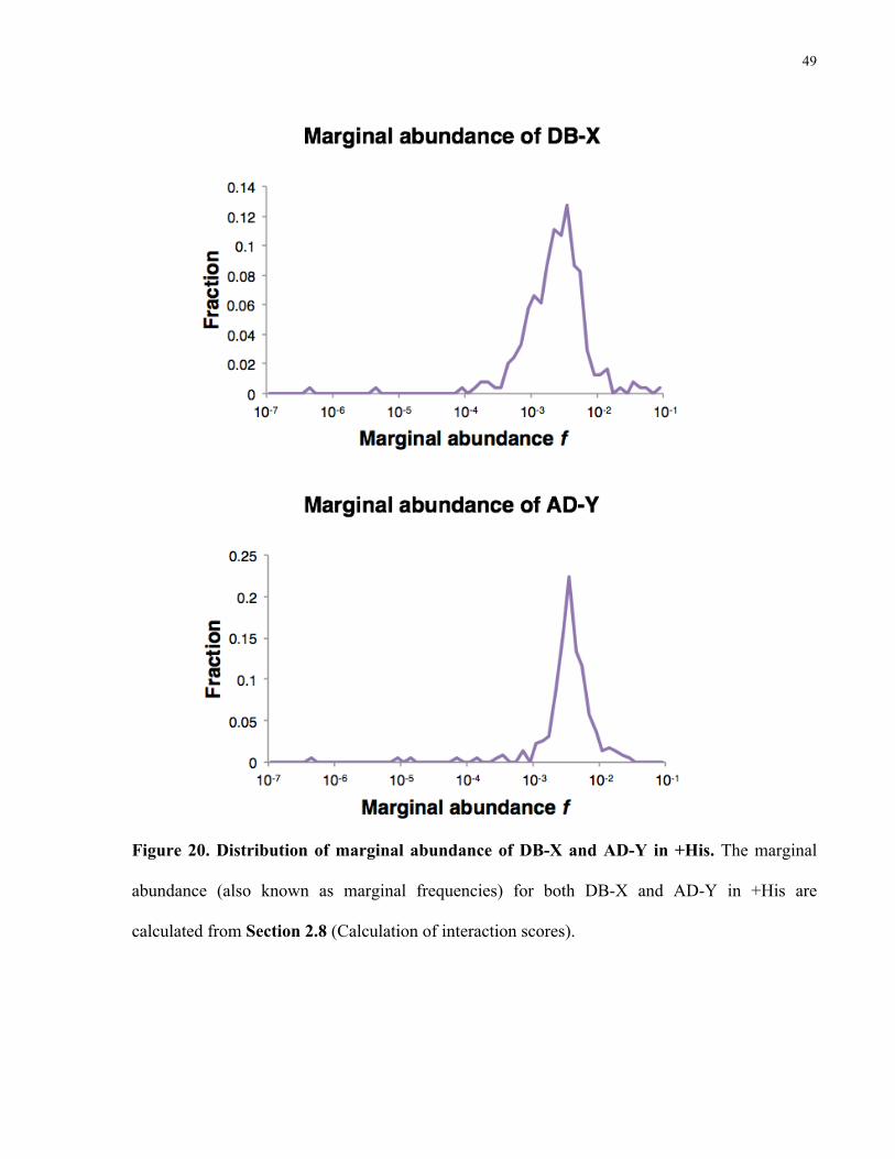
marginal frequencies of +His (Figure 19), -His (Figure 21) and +3AT (Figure 22). The raw

barcode counts in the +His condition ranged from 0 to 5.95 on a log10 scale (or 0 to 890,000).

The distributions of the marginal frequencies of the DB-X and AD-Y pools in the +His are

shown in Figure 20 (see Section 2.8 (Calculation of interaction scores) for more details for

calculating the marginal frequencies). The majority of the marginal frequencies range between

10-2 and 10-3. Please see Figure 23 for the overlap of positive interactions between –His

condition and +3AT condition.

The expected interactome (BioGRID Y2H datasets) from all of the DNA damage repair

proteins present in the screen are shown in Figure 24.

. Please see Appendix 7.5 for the top 200 interactions and their corresponding

normalized scores.

48

Figure 19. Marginal counts of the BFG-Y2H screen without histidine supplements. This is a

non-selective condition, giving an overall view of the complexity of the diploid strains, as well

as providing the background values for normalization of the scores in the selective conditions

downstream. The values in the heatmap are the marginal frequencies transformed to a log10

scale. The PRS controls are within the square in the upper-left corner. The DB-X (prey) proteins

are on the Y-axis and the AD-Y (bait) proteins are on the X-axis. Dark blue represents high

marginal frequencies, whereas white represents low marginal frequencies.

49

Figure 20. Distribution of marginal abundance of DB-X and AD-Y in +His. The marginal

abundance (also known as marginal frequencies) for both DB-X and AD-Y in +His are

calculated from Section 2.8 (Calculation of interaction scores).

50

Figure 21. Normalized scores of the BFG-Y2H screen without histidine supplements. This is

a selective condition whereby positive protein interactions and de novo autoactivators are

captured. The values in the heatmap been normalized against the +His matrix and also

normalized within each row. They have also been transformed to a log10 scale. The PRS

controls are within the square in the upper-left corner. The DB-X (prey) proteins are on the Y-

axis and the AD-Y (bait) proteins are on the X-axis. Dark blue represents high normalized

scores, hence positive protein interaction candidates. White represents low normalized scores,

hence, no protein interaction candidates.

51

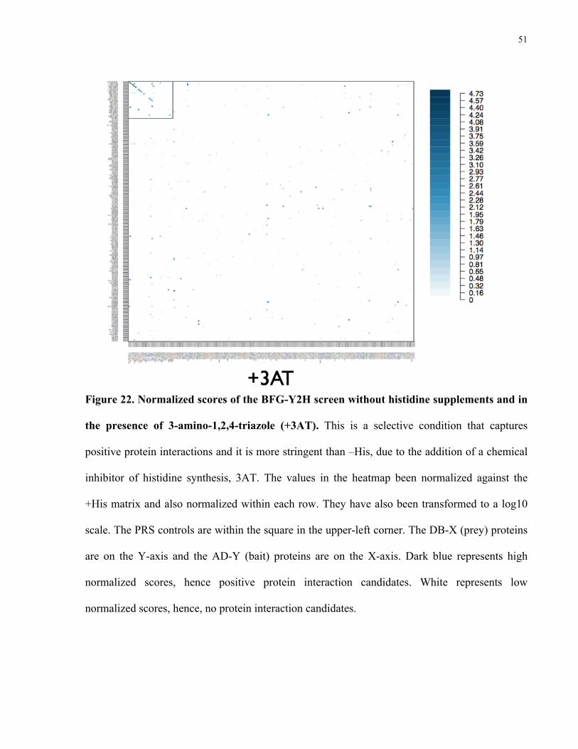
Figure 22. Normalized scores of the BFG-Y2H screen without histidine supplements and in

the presence of 3-amino-1,2,4-triazole (+3AT). This is a selective condition that captures

positive protein interactions and it is more stringent than –His, due to the addition of a chemical

inhibitor of histidine synthesis, 3AT. The values in the heatmap been normalized against the

+His matrix and also normalized within each row. They have also been transformed to a log10

scale. The PRS controls are within the square in the upper-left corner. The DB-X (prey) proteins

are on the Y-axis and the AD-Y (bait) proteins are on the X-axis. Dark blue represents high

normalized scores, hence positive protein interaction candidates. White represents low

normalized scores, hence, no protein interaction candidates.

52

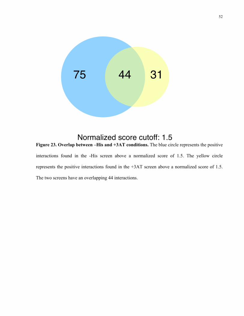
Figure 23. Overlap between –His and +3AT conditions. The blue circle represents the positive

interactions found in the -His screen above a normalized score of 1.5. The yellow circle

represents the positive interactions found in the +3AT screen above a normalized score of 1.5.

The two screens have an overlapping 44 interactions.

44 3175

Normalized score cutoff: 1.5

53

Figure 24. The expected interactome. The expected interactome from BioGRID Y2H

interactions. The DNA damage repair proteins that have not been barcoded successfully have

been removed from this interactome.

54

3.5 Benchmarking for pairwise retesting

A threshold is needed to prioritize and select positive protein interaction candidates for

pairwise retesting. This threshold should optimize the balance between false negatives and false

positives, which means that a set of true interactions is needed for benchmarking. Arguably, the

highest quality Y2H screen of the yeast proteome was done by Yu et al (2008)43. The

background strains and the plasmids used by Yu et al. are also the closest to my strains used in

this screen. Therefore, the overlap between the positive interactions from Yu et al. and the DNA-

damage repair proteins in the matrix was used as a reference set of high-confidence PPIs (11

positive interactions). The true positives also include the previously mentioned PRS controls

from the Vidal lab I pairwise retested to be positive interactions (17 true positive interactions,

Figure 18). I plotted precision, recall and the Matthews correlation coefficient44 (MCC). The

MCC is a measurement of the quality of binary classifications. It optimizes between precision

and recall, and it has a range of values from -1 (disagreement between prediction and

observation) to 1 (perfect agreement between prediction and observation). The maximum

precision is around 0.5. The best MCC was 0.33, corresponding to a normalized score of 3.25,

which identified 30 candidate protein interactions.

55

Figure 25. Prediction performance of the reported BFG-Y2H positive protein interactions

for the –His condition benchmarked against Yu et al. 43. The “true positive” interactions are

the union of the PRS controls from the Vidal lab and the positive interactions from Yu et al.

MCC denotes Matthew correlation coefficient, which optimizes between precision and recall.

56

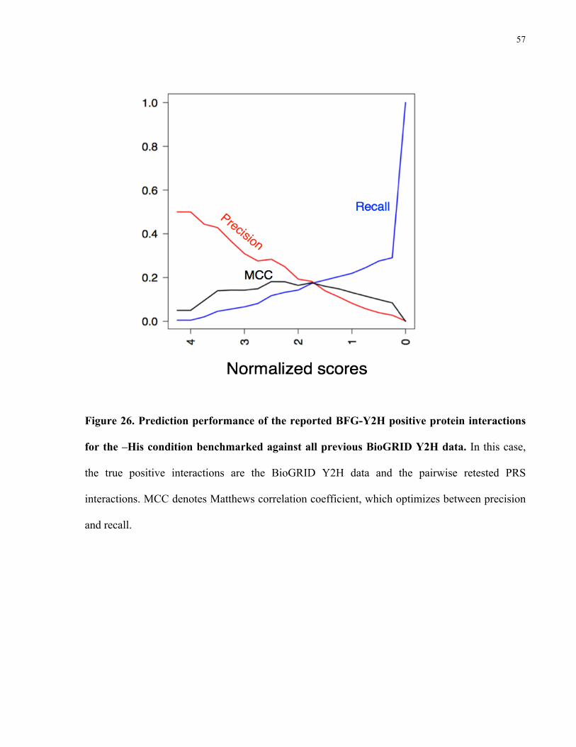
In addition to the high-quality Y2H screen of the yeast proteome from Yu et al (2008)43,

many other high-throughput Y2H datasets are also included in BioGRID (such as Uetz et al.45

and the “core” subset of Ito et al.46, where only interactions that tested at least twice were

included). Therefore, I benchmarked my dataset against all of the Y2H datasets available in

BioGRID (128 positive Y2H interactions), as well as the previously pairwise retested PRS pairs

from the Vidal lab (17 PRS Y2H interactions). I plotted precision, recall and the MCC (Figure

26). The maximum precision is around 0.5 as in the previous comparison (Figure 25). The

maximum MCC was around 0.18, which corresponds to a normalized score of 2.5, yielding 81

candidate interactions.

57

Figure 26. Prediction performance of the reported BFG-Y2H positive protein interactions

for the –His condition benchmarked against all previous BioGRID Y2H data. In this case,

the true positive interactions are the BioGRID Y2H data and the pairwise retested PRS

interactions. MCC denotes Matthews correlation coefficient, which optimizes between precision

and recall.

58

3.6 Pairwise retesting on BFG-Y2H candidate interactions

From the two precision and recall curves, it appears that benchmarking against the Yu et

al.43 dataset yielded better MCC and recall values. However, using the best MCC score of 0.33 as

a cutoff, it would mean that we would only test the top 30 interactions from the BFG-Y2H

primary hits. Instead, 52 positive interactions from the primary BFG-Y2H screen were

arbitrarily selected amongst the top 185 hits and their interactions were tested with pairwise

retesting (Section 2.7 Pairwise retesting). The pairwise retesting results are shown in Figure 27;

46% (24) of the 52 candidate pairs were confirmed by pairwise retesting. Of these 24 confirmed

interactions, 17 of them were novel relative to the Yu et al.43 dataset, and seven were novel

compared to all the Y2H data from BioGRID (Table 3). After doing a thorough search, five of

these seven confirmed interactions were novel (have not been previously reported by previous

literature).

I created an interactome map with interactions that were confirmed by pairwise retesting

(Figure 28). The colour of the edges represent where the protein interaction was seen previously

in the literature. The width of the edges represents the normalized interaction score. All novel

interactions are shown in red.