Identifying Demand Responses to Illegal Drug …economic/RePEc/pdf/tul1312.pdfIdentifying Demand...

Tulane Economics Working Paper Series

Identifying Demand Responses to Illegal Drug Supply Interdictions

Scott CunninghamDepartment of Economics

Baylor UniversityWaco, TX

scott [email protected]

Keith FinlayDepartment of Economics

Tulane UniversityNew Orleans, LA

[email protected]

Working Paper 1312March 2013

Abstract

The optimality of supply interventions for addictive drugs is a function of demand responses to price,enforcement costs, and the relative size of external costs. Researchers need credible estimates of demandresponses, but most research designs use price series affected by law enforcement actions. We presentplausibly causal estimates of the price elasticities of demand for various drugs when enforcement costsare relatively low. We exploit arguably exogenous shocks to methamphetamine supplies to identifythe effect of methamphetamine prices on demand for methamphetamine, alcohol, cocaine, heroin, andmarijuana. Methamphetamine demand is price inelastic with substantial substitution to other drugs.

Keywords: illegal drugs, addiction, demand, substitution, War on Drugs, methamphetamineJEL: I12, I18, K42

Identifying Demand Responses toIllegal Drug Supply Interdictions

Scott Cunningham and Keith Finlay∗

February 23, 2013

Abstract

The optimality of supply interventions for addictive drugs is a function of demand responsesto price, enforcement costs, and the relative size of external costs. Researchers need credibleestimates of demand responses, but most research designs use price series affected by law en-forcement actions. We present plausibly causal estimates of the price elasticities of demandfor various drugs when enforcement costs are relatively low. We exploit arguably exogenousshocks to methamphetamine supplies to identify the effect of methamphetamine prices on de-mand for methamphetamine, alcohol, cocaine, heroin, and marijuana. Methamphetamine de-mand is price inelastic with substantial substitution to other drugs.

Keywords: illegal drugs, addiction, demand, substitution, War on Drugs, methamphetamineJEL codes: I12, I18, K42

∗Department of Economics, Baylor University, Waco, TX, 254-710-4753, [email protected]; and Depart-ment of Economics, 206 Tilton Hall, Tulane University, New Orleans, LA 70118, 504-862-8345, [email protected] is the corresponding author. We thank the National Science Foundation (award SMA-1004569), Robert WoodJohnson Foundation (award 70509), and Tulane Research Enhancement Fund for support. Both authors have con-tributed to the data collection, analysis, and writing of this manuscript. Neither author has a financial interest or con-flict of interest related to the findings reported in this paper. Data and codes can be obtained from the correspondingauthor.

1 Introduction

Costs related to the prohibition of addictive drugs and the enforcement of drug laws are as much

as $40 billion annually in the US (Miron and Waldock, 2010). The US incarceration rate per 100,000

residents grew from 100 in 1980 to 492 in 2011, while the share of prisoners convicted of drug

offenses increased from 22% to 48% during the same period (Blumstein and Beck, 1999; Carson

and Sabol, 2012). The efficacy of enforcement-oriented interventions is uncertain given evidence

of diminishing returns to imprisonment in reducing crime including drug use and trafficking

(Johnson and Raphael, 2012). To evaluate the optimality of alternative policies for addressing

the public health costs of addictive drugs, researchers need credible estimates of the demand

responses to those policies. Enforcement strategies continue under the assumption that those

efforts increase prices sufficiently to reduce demand. In this paper, we present plausibly causal

estimates of the price elasticities of demand for various drugs in a setting in which enforcement

costs are relatively low.

The large economic costs of substance abuse include the impact of addiction on quality of

life, the crowd out of public resources, the relationship of drugs to crime, and the impacts on the

families of users.1 Methamphetamine, the focus of this study, now ranks second behind marijuana

as the most widely used illegal drug with damages that originate from its production and use.

Public health costs such as child maltreatment, foster care admissions, environmental damage,

and hospitalization greatly contribute to methamphetamine’s high social cost—estimated at $23.4

billion in 2005 (Nicosia et al., 2009).

Methamphetamine is relevant for evaluating drug policy because its economic costs are large

and its production process may allow cost-effective supply interdictions. Unlike many other

illegal drugs, methamphetamine (meth) is synthesized from chemical precursors produced in con-

centrated global input markets. Restricting precursor supplies can decrease quantity and increase

price without increasing imprisonment. Compared to public awareness campaigns targeted at

meth demand (Anderson, 2010), precursor controls have been temporarily successful at reducing

demand (Dobkin and Nicosia, 2009; Cunningham and Finlay, 2013). Precursor controls may have

only temporal effectiveness because of large potential profits in underground meth markets and

1See Cook and Moore (2000); Chaloupka and Warner (2000); and Cawley and Ruhm (2011) for a review of the socialcosts of substance abuse and risky behaviors.

1/ 31

incomplete regulation of precursor supply chains.

It is surprising how few credible estimates of demand elasticities for illegal drugs exist given

its importance in the design of optimal drug policy (Becker et al., 2006). The simultaneity of

supply and demand for each drug confounds estimates of demand elasticities as causal measure

of demand response to price changes. For example, suppose that the government chooses a

prohibition and enforcement policy for reducing illegal drug consumption, then increases the

number of police tasked with arrested drug traffickers and users. This strategy, potentially un-

observable to the researcher, will both increase production costs for providers and increase the

risk of punishment for users.

Our research design overcomes these confounds through an instrumental variables strategy

that exploits two large, exogenous meth price shocks caused by two federal interdictions that

created temporary shortages of the key chemical precursors used in meth production. To estimate

own- and cross-price elasticities of demand for drugs, we collect monthly data on substance abuse

treatment admissions as a proxy for the number of substance users, retail drug prices, and a variety

of other potentially relevant factors for US states from January 1995 to December 1999 and estimate

instrumental variables models of the effect of meth prices on treatment admissions for various

substances. With this instrumental variable strategy, we show that the demand curve for meth is

downward-sloping but inelastic and that alcohol, heroin, cocaine, and marijuana are all temporary

substitutes for meth. At their peak, cross-price elasticities are about one-third the size of the own-

price effects and attenuate within six months from the start of the price shocks.

Using the own-price elasticity of −0.25 and assuming zero marginal costs of enforcement, we

show that precursor control is socially optimal if the negative social externality from meth is more

than four times its private value to users. Meth may have relatively large social costs. But if

marginal costs of enforcement are positive and precursor controls are only temporarily effective,

then precursor controls are less likely to be cost effective (e.g., precursor control burdens legitimate

medical consumers). The next section provides background of drug demand and meth interven-

tions. We then describe the empirical model and the data, discuss our results, and conclude.

2/ 31

2 Background

Optimal drug enforcement

In a normative economic approach to drug policy, a government would choose policies that mini-

mize the social costs of drug use. Becker et al. (2006) contrast the social welfare under a free market

for drugs with a regime where drug quantities are reduced through enforcement and punishment.

They show that the optimal level of enforcement depends on whether demand is inelastic, the

size of the negative externalities from drug consumption and the costs of enforcement. If the

social planner wishes to choose a level of enforcement, E, that maximizes the net benefits of

consumption minus the sum of production and enforcement costs, then the following first-order

condition must hold in equilibrium:

C1 + C2(Q+ EdQ

dE) + C3(θ

dQ

dE+Q

dθ

dE) = Vq

dQ

dE−MR

dQ

dE, (1)

where Q is the quantity of drugs consumed, θ is the odds ratio expression of the probability of

arrest, Vq is the marginal social willingness-to-pay for illegal drug consumption, and MR is the

marginal revenue for drug suppliers. The marginal cost of enforcement contains both a public

good component, C1, that is invariant to the quantity of drugs, and a private component, C2,

that varies with quantity. The final component of the marginal cost of enforcement is C3, which

measures the costs of punishing arrested users. The right-hand side of equation 1 measures the

marginal benefit of reduced consumption.

If we assume that marginal costs of enforcement are zero, we can rearrange Equation 1 so that

the role of price elasticity of demand in optimal drug policy is more transparent:

VqP

= 1 +1

εd, (2)

where εd is the price elasticity of demand for drugs and P is the price paid by consumers for

drugs. As price equals the private willingness to pay in competitive markets, the left-hand side

of Equation 2 equals the ratio of marginal social to private value of illegal drug consumption.

If demand is inelastic, then both the right-hand side and left-hand side of Equation 2 must be

3/ 31

negative in order for non-zero levels of drug enforcement to be optimal. This requires negative

externalities in consumption, Vq < 0, given that price is non-negative.

If demand is inelastic and the negative externalities in consumption are relatively small, then

the free market level of consumption is socially optimal. This is because production and dis-

tribution costs are rising as output falls at a loss in social utility from reduced consumption.

If meth demand is inelastic, then government intervention is justified if and only if the social

value of meth consumption is “very negative”. Thus even in a world where the marginal costs of

enforcement are essentially zero, inelastic demand implies that enforcement is optimal only when

there are substantial negative externalities from consumption, and even then, quantity restrictions

will absorb a considerable amount of resources.

If we relax the zero marginal cost assumption, we find marginal enforcement costs are rising

as demand becomes less elastic. This is because consumption falls more slowly when demand is

inelastic, and since expenditures on apprehension and punishment depend on output, a slower

fall in output with inelastic demand will cause enforcement expenditures to grow more rapidly.

Therefore we can conclude that falling consumption causes total production costs and enforce-

ment costs to rise more rapidly when demand is inelastic.

There is some pessimism about the efficacy of supply-side interventions among researchers.

An early study by Rydell and Everingham (1994) suggested that supply-side strategies may not

be cost effective. Prohibition and enforcement have even been shown to reduce prices contrary to

economic intuition (DiNardo, 1993; Yuan and Caulkins, 1998), but this result may be explained by

nonpecuinary aspects of market operation such as violence that impose externalities on suppliers

(Caulkins et al., 2006). Given the high social costs of incarceration, this evidence is consistent with

evidence that enforcement strategies may not be cost effective (Kuziemko and Levitt, 2004).

These studies rarely use research designs capable of identifying the causal effects of enforce-

ment. One exception is DeSimone (2001) who estimates the causal effect of cocaine prices on crime

using instrumental variables. He instruments for price with measures of wholesale supply factors

and retail enforcement intensity. But if enforcement determines crime directly, these instruments

are possibly not excludable from the second-stage equations. Nicosia et al. (2009) estimate the

causal effect of meth on crime using the 1995 ephedrine interdiction for California and find no

effect. Cunningham and Finlay (2013) use state-level data and both the 1995 and 1997 precursor

4/ 31

interventions and identify a positive elasticity foster care admission with respect to meth use.

Estimated price elasticities of drug demand

The own- and cross-price elasticities of short and long-run demand enable policymakers to fore-

cast the impact of and evaluate the cost effectiveness of a given intervention. It would also provide

some guidance as to when demand-side interventions may be the more cost effective approach.

Most economic studies suggest that addictive substances are consumed on the inelastic portion

of demand. For example, Chaloupka and Warner (2000) and Gallet and List (2003) agree that

most studies estimate the own-price elasticities for tobacco to be −0.3 to −0.5. Similarly, Cook

and Moore (2000) notes that the average own-price elasticity for beer, wine and spirits is −0.35,

−0.68, and −0.98, respectively, which is also found in more updated reviews such as Wagenaar

et al. (2009). Gallet (2007) finds a median elasticity for alcohol of −0.55 across 132 studies.

In comparison, our knowledge about cross-price elasticities for addictive substances is much

less developed. Few economists have attempted to calculate cross-price elasticities for tobacco,

and those which do exist typically only focused on the within-tobacco categories and various

intensive margins, such as higher tar cigarettes and smokeless tobacco products. Ohsfeldt and

Boyle (1999) estimates the cross-tax elasticity of snuff use with respect to cigarette prices at 0.98

for males older than 16, whereas Decker and Schwartz (2000) estimated a negative cross-price

elasticity for cigarettes and alcohol reflecting complementarities in consumption.

Knowledge of the elasticities of demand for illicit substances is less mature than our knowl-

edge of the same for alcohol and tobacco due both to the smaller number of economic studies

on illicit substances and the unique challenges associated with studying illicit drugs. There is

considerable variation in the magnitude of elasticities of demand for heroin and cocaine. For

example, Dave (2008) estimates own-price elasticities of cocaine and heroin at −0.27 and −0.10,

respectively, using emergency department visits, but Caulkins (2001) estimates an own-price elas-

ticity of demand for cocaine and heroin at −1.3 and −0.84, respectively, using hospitalizations.

Saffer and Chaloupka (1999) estimated−0.82 to−1.03 for heroin prevalence elasticities of demand,

and −0.28 to −0.44 for cocaine. Liu et al. (1999) find evidence that opium is inelastic in the

short-run (−0.48), but elastic in the long-run (−1.4), whereas Ours (1995) estimates an elasticity

5/ 31

of −0.7 and −1.0 in the short and long-run, respectively. Differences in the magnitudes are

due to a combination of data aggregation, identification strategy, the time dimension and the

choice of the proxy. Cross-price elasticities of demand for drugs have rarely been attempted,

and to our knowledge, no one has found strong statistical evidence that they exist. Saffer and

Chaloupka (1999) and Dave (2006) both attempted to estimate cross-price elasticities, but neither

found statistically significant results. To our knowledge, there have been no studies of drug

demand responses to meth prices.

Methamphetamine and precursor control

A recent study by the Rand Corporation calculates that the total economic costs of meth produc-

tion and use were $23.4 billion in 2005. While the majority of this calculation can be attributed to

reduced quality of user lives, a large share of total costs were externalities to nonusers caused by

reduced worker productivity, harm to children, crime, and pollution (Nicosia et al., 2009). Only

a few studies have attempt to estimate the causal effect of meth use on public health outcomes.

Dobkin and Nicosia (2009) find no evidence that meth causes crime, whereas Cunningham and

Finlay (2013) estimate a positive elasticity of foster care admissions with respect to meth use due

to increased child neglect and abuse. Meth dependency affects user brain chemistry with evidence

of long-term increases in psychosis, paranoia, and aggression (Rawson et al., 2001).

Meth is synthesized from a reduction of ephedrine or pseudoephedrine, the active ingredients

in commonly used cold medicines, so meth production requires access to legitimate input markets.

While cold medications can be purchased at retail pharmacies, large quantities of bulk precursors

can only be obtained in wholesale markets that are subject to chemical trafficking regulations.

These chemicals are not produced domestically. Suo (2004) reports that in 2004, only nine interna-

tional factories manufactured the bulk of the world supply of ephedrine and pseudoephedrine.

Since these precursors are distributed and packaged in different forms, the history of precursor

control is one in which meth producers innovate around narrow restrictions on precursors created

by federal legislation. In 1988, Congress passed the Chemical Diversion and Trafficking Act that

gave the DEA the authority to control the wholesale distribution of precursors used to produce

illegal drugs, such as meth, LSD, and PCP. The statute required bulk distributors of ephedrine and

6/ 31

pseudoephedrine to notify drug enforcement authorities of imports and exports and keep records

of purchasers (Suo, 2004; [US DEA] United States Drug Enforcement Administration, 1997). All

tablet forms of ephedrine and pseudoephedrine medical products, however, were exempt—a legal

loophole that drug trafficking organizations quickly exploited.

The primary sources of precursors following the 1988 regulation were wholesale and mail

order distributors of ephedrine tablets. In the early 1990s, there was little use of pseudoephedrine

as a precursor. In 1994, ephedrine was identified as the source material in 79% of meth lab seizures,

while pseudoephedrine was only found in 2% (Suo, 2004). Congress sought to close the legal

loophole in 1993 by passing the Domestic Chemical Diversion Control Act, which became effective

August 1995. This new regulation provided additional safeguards by regulating the distribution

of products that contained ephedrine as the only active medicinal ingredient ([US DEA] United

States Drug Enforcement Administration, 1995; Cunningham and Liu, 2003). The new legislation

ignored pseudoephedrine tablets, so traffickers soon took advantage of the omission by substi-

tuting towards pseudoephedrine as a precursor. By 1996, pseudoephedrine was found to be the

primary precursor in almost half of meth lab seizures ([US DEA] United States Drug Enforcement

Administration, 1997). From 1996 to 1997, pseudoephedrine imports grew by 27% while sales

of all cold medications grew only 4% (Suo, 2004). As a consequence, the DEA sought greater

controls over pseudoephedrine products. The Comprehensive Methamphetamine Control Act of

1996 went into effect between October and December 1997 and required distributors of almost all

forms of pseudoephedrine to be subject to chemical registration ([US DEA] United States Drug

Enforcement Administration, 1997).

In the short-run, these precursor controls may have been the most successful supply-side

interdictions in the history of US drug enforcement (Dobkin and Nicosia, 2009).2 Evidence of

this can be seen in its effect on meth prices. We construct a monthly price series for a pure gram

of meth, heroin and cocaine using the DEA’s System to Retrieve Information from Drug Evidence

(STRIDE) database.3,4 Our monthly price series is from January 1995 to December 1999. We use

2The long-run effects of these wholesale regulations were more muted, as meth producers appear to have adaptedto the increased restrictiveness of domestic precursor acquisition by relocating operations out of the US, shifting to newtechnologies, and substituting from wholesale to retail purchases (e.g., pharmaceutical purchases of cold medicationswith active pseudoephedrine).

3See Appendix A for a more detailed explanation of the construction of the drug price series used in the paper.4There is a debate about the ability of researchers to recover the distribution of market prices from STRIDE because

its sampling is determined by law enforcement actions. See Horowitz (2001) for the critical argument and Arkes et al.

7/ 31

an empirical method to identify the windows during which each intervention was effective by

first regressing real expected meth prices onto a cubic time trend. We then add a single-month

fixed effect for each month after the intervention began—retaining only those that are statistically

significant. We repeat these steps until the last contiguous, post-intervention month dummy vari-

able is statistically insignificant. The Domestic Chemical Diversion Control Act became effective

in August 1995, and our method identifies deviations in price trends from September 1995 until

February 1996. The Comprehensive Methamphetamine Control Act became effective between

October and December 1997, and our model identifies detectable deviations in price trends from

April 1998 to March 1999.5

Figure 1 shows the median monthly expected price of meth, heroin, and cocaine relative to

their respective median values in January 1995. We mark the window of the two federal inter-

dictions’ efficacy with vertical bars. The 1995 shock caused meth prices to more than quadruple

in a brief period of time. Prices returned to pre-interdiction levels after six months. The 1997

interdiction was comparatively smaller in magnitude, but caused meth prices to increase over

their pre-interdiction levels for twelve months. These large but temporary disruptions in meth

markets are key to our identification of the demand elasticities. For comparison, we present

expected price of cocaine and heroin (relative to their January 1995 median values) on the same

graph. There is no similar change in median heroin or cocaine prices relative to pre-interdiction

levels during either intervention suggesting that the effect is the result of unique factors in meth

markets.6

3 Estimation, identification, and data

We are interested in the causal effect expressed as an elasticity measure of meth prices on the

demand for meth (m), alcohol (a), marijuana (mj), cocaine (c), and heroin (h) (with drugs indexed

(2008) for a rebuttal.5Our empirical method for dating the interventions in this paper is similar to previous studies. Dobkin and Nicosia

(2009) use a four-month window for the 1995 intervention, but they limit their attention to California where the methmarket is the most sophisticated and producers are arguably more adaptable. Cunningham and Liu (2003, 2005) usesix months for the 1995 intervention (August 1995–January 1996).

6Since 2000, there have been a variety of state-level precursor controls, ranging from quantity restrictions toelectronic tracking of purchases to doctor prescription requirements. Since producers can obtain inputs fromneighboring states, the price effects of these interventions are smaller and evidence suggests the demand responsesare also smaller (Nonnemaker et al., 2011; [US GAO] United States Government Accountability Office, 2013).

8/ 31

by i). Consider linear demand equations of the form:

ln(Qist) = βiOLSln(Pmst ) + γiXst + εist ∀i ∈ {m, a,mj, c, h}, (3)

where Q is self-referred treatment admissions, Pm is the retail price of a pure gram of meth (m),

and ε is the error term. The vector X includes state fixed effects, month-of-year effects, a national

time trend, other state-level drug prices if they are available, the state population aged 15–49 years,

and the state unemployment rate. The unit of observation is state s in month t, and all regressions

are weighted by the population aged 15–49 years. The parameters of interest are βm, the own-

price elasticity of demand for meth, and the βi 6=ms, the cross-price elasticities of demand for the

other drugs.

Price and quantity in Equation 3 are observed in market equilibrium. The simultaneity of

supply and demand for each drug confounds the interpretation of βiOLS as a causal measure of

the demand response to price changes. For example, suppose that the government chooses a

prohibition and enforcement policy for reducing illegal drug consumption, then increases the

number of police tasked with arrested drug traffickers and users. This strategy, potentially unob-

servable to the researcher, will both increase production costs for providers and increase the risk

of punishment for users. The equilibrium prices and quantities reflect both of these responses, so

βiOLS may be biased by the omission of unobserved law enforcement variables.

In order to identify the demand response to drug price changes, we use an instrumental

variables strategy and estimate a two-stage least squares (2SLS) model. Our instrumental variable

is an indicator variable equal to one for months when the 1995 and 1997 federal interventions had

significant disruptions on meth markets and zero for all other months (as described above). The

first-stage meth price model is:

ln(Pmst ) = ζZt + πXst + ωst, (4)

where ωst measures the unobserved determinants of meth prices in state s and month t. The

second-stage demand model becomes:

ln(Qist) = βiIVln(P̂mst ) + γ̃iXst + ε̃ist ∀i ∈ {m, a,mj, c, h}, (5)

9/ 31

where ln(P̂mst ) is the fitted log meth price from our first stage model. To identify βiIV, the instrument

Zt must be correlated with meth prices, which we establish in Figure 1. Identification also requires

that the instrument only affect drug demand through its affect on meth prices. Although we know

of no contemporaneous increases in law enforcement effort during the intervention periods, we

focus on self-admitted treatment admissions to isolate the demand response that is most likely to

be independent of police effort.7

Our measure of demand is a proxy and deserves a discussion. Proxies are often used in illegal-

drug research because of the inherent difficulty in observing underground markets and because of

underreporting of illegal behavior in surveys of individual behavior. We also need monthly data

to properly time the meth precursor interventions and admissions to drug treatment facilities

are a frequent event that can be aggregated to the state-month level. Admissions are likely to

be correlated with drug use, but must also satisfy other characteristics for us to consider βiIV an

elasticity of drug (use) demand. Suppose that a constant proportion, 0 < ζ < 1, of total meth users

are in treatment at any given time with an multiplicative iid measurement error η ∼ lnN(0, σ2η).

As long as ζ and η are not systematically different during the precursor interventions, ζ will be

absorbed by the constant term and η will be absorbed by the error term, and we can still identify

the elasticities of interest.

To estimate Equations 3–5, we combine state-month data from a variety of sources. We choose

a sample period of January 1995 to December 1999 for all datasets. This starts eight months

before the first intervention and ends nine months after the second intervention. We construct an

estimated price series for a pure gram of meth, heroin and cocaine/crack using the DEA’s System

for the Retrieval of Drug Evidence (STRIDE) dataset.8 All prices are adjusted to 2002 dollars using

the All Urban CPI series. Drug price observations do not occur in every state-month cell. To

impute price observations for missing cells, we take price averages from higher level geographic

areas, moving from states, to census divisions, to census regions, and finally to national price

series. This imputation should reflect the price users must pay in a particular state. We show a

comparison of both sets of price series in Table 1. The two sets have similar means but the series

7The local average treatment effect interpretation of the IV parameter is a consideration if price responses tointerventions are systematically different in intervention periods. We have no reason to believe heterogeneity indemand responses to price exists, but the first-stage monotonicity requirement is likely to be satisfied in any case.

8Most marijuana observations in STRIDE are due to seizures. As a result, they are missing price data. Marijuanapurity also is not available, making it impossible to generate a reliable price or purity series using these data.

10/ 31

with imputed prices have smaller variances.

Drug treatment admissions data comes from the Department of Substance Abuse and Mental

Health Administration’s Treatment Episode Data Set (TEDS). TEDS records the universe of all

federally funded treatment inpatient or outpatient facilities. Patients admitted are interviewed to

determine the routes of admission, as well as which substances were used at their most recent

treatment episode. We use the number of treatment admissions by substance abuse category as

proxies for the following substances: meth, alcohol, cocaine/crack, heroin and marijuana. We

report both the total admissions aggregated over all routes of admissions as well as the number of

self-referred admissions for each substance abuse variable of interest.

The population of those aged 15–49 years in each state in 1,000s comes from SEER (2011). State-

level unemployment rates were obtained from the Current Population Survey. We also include

state cigarette taxes measured as real dollars per cigarette pack (Orzechowski and Walker, 2011).

4 Results

All models use the log of the treatment admissions as dependent variables and log of meth prices

as the independent variable. The regressions all have a log-log form, so the coefficients are

approximately equal to elasticities. Our meth variable includes all mentions of meth, but our

other substance abuse variables exclude any cases where meth was mentioned so as to avoid

double counting.9 We use only self-admission cases because self-admit are those individuals who

would be price responsive.10

We estimated Equation 3 using five different outcome variables: meth (Table 2), alcohol (Table

3), heroin (Table 4), crack and powder cocaine (Table 5) and marijuana (Table 6). The first two

columns of each table use the same specification, and we report OLS and 2SLS estimates for

comparison. Our 2SLS models are identified from the temporal shocks to meth prices created

by the two precursor interdictions. As such, it would be useful to see how reduced demand for

meth and substitution toward alternative drugs changes over time. In a series of figures, we plot9TEDS admissions list their primary, secondary and tertiary substance used at the most recent episode, so it’s

possible for alcohol cases to occur with meth. As we do not want to bias downward estimates of cross-price elasticitiesby including cases where meth appeared with other drugs, we focus on cases where meth is not mentioned at all, whichwe view as a conservative estimate.

10Criminal justice referrals, for instance, are usually instances where a judge assigned treatment to a defendant. Thetheory of demand would not suggest judges are making decisions in response to price fluctuations.

11/ 31

the coefficient estimates with different leads to illustrate the transition of the short-run elasticity to

the medium-run elasticity over a six-month spell (Figures 2 and 3). These models are of the form:

ln(Qis,t+L) = βiIV,Lln(P̂mst ) + γ̃iLXst + ε̃is,t+L ∀i ∈ {m, a,mj, c, h}, (6)

where the demand leads run from L = 0 to 6.

Table 2 reveals a negative point estimate for the own-price elasticity of meth demand. The

first stage results show that the real price of meth rose 63 log points during the two interventions,

or 87.7 percent.11 As OLS and 2SLS both agree on the sign of the elasticity, we will report the

2SLS estimates since they are better identified. While meth has inelastic demand in all seven

specifications, consumer responsiveness to prices increases as we use higher order leads. The con-

temporaneous elasticity is −0.06. Within two months, the elasticity has doubled, and within four

months it has quadrupled. The upper bound elasticity of −0.22 to −0.25 is achieved within four

months time. We present these estimates with 90% confidence intervals in Figure 2 as well. While

meth demand is becoming more elastic over time, as theory would suggest, we can only say that

the elasticity reaches a max of −0.25 using the six month price leads. We do not feel comfortable

exploring beyond six months given the exogenous price changes caused by the supply disruptions

were temporary.

Since these are the first estimates of the own-price meth elasticity, they are not directly com-

parable to other estimates of the same parameter. But compared to the estimated elasticities for

other drugs, our estimates suggest that meth is one of the more inelastic drugs estimated to date.

The central tendency among all published elasticities for illegal drugs is negative one-half with

a large standard deviation (Becker et al., 2006). Our medium-run own-price elasticity of −0.25 is

most comparable to Dave (2006) who estimated a contemporaneous own-price elasticity of cocaine

using annual hospitalizations as a proxy of −0.27.

Next we discuss our estimates of various cross-price elasticities with respect to meth prices.

The most common substance reported by treatment patients is alcohol by a significant margin.

Using only self-referred alcohol admissions, the mean number of monthly alcohol mentions in

TEDS is 613 for this period of time compared to 71 for meth (Table 1). It is perhaps in part for this

11e0.63 = 1.877

12/ 31

reason that the cross-price elasticities that we estimate are relatively small given the large volume

of alcohol mentions in the data. Our evidence suggests that alcohol is a substitute for meth in the

short-run, but that substitution dissipates after five months. The cross-price elasticity of demand

for alcohol with respect to meth prices reaches a peak of +0.11 after two months. Assuming a

baseline of 613 alcohol admissions, this implies that an 87.7% increase in prices caused by the

intervention caused alcohol admissions to increase 9.65%, or 59 additional alcohol admissions.

The shape of the cross-price elasticity for each of the seven specifications is presented in Panel A

of Figure 3.

For each alternative substance category, we find cross-price elasticities that are both positive

and shaped like our alcohol estimates over time. The differences that we find typically depend

on how soon the responsiveness tapers off. Heroin, for instance, reaches a similar level to that

of alcohol, but begins declining sooner becoming marginally significant by the third month. The

peak cross-price elasticity of demand for heroin is +0.10, which is reached in months one and

two. It declines soon thereafter becoming statistically indistinguishable from zero by the fourth

month and zero in absolute value at the sixth month. We present the elasticity for heroin in Panel

B of Figure 3. As can be seen when the two are side by side, alcohol appears to have been more

responsive than heroin in the medium run.

The cross-price elasticity of demand for powder cocaine and crack is, like the others, positive

and attenuates after its peak. Although we cannot observe past the six-month window, the tra-

jectory suggests cocaine and meth may only be temporarily substitutable. The peak value of the

cross-price elasticity of demand for cocaine is +0.12 which corresponds to the fourth month lead.

This is presented in Panel C of Figure 3, as well. Finally, we present our estimates for marijuana

elasticities. We find that marijuana demand grows to +0.09 by the third month after which it

declines and is statistically insignificant at the sixth month. This shape is presented in Panel D of

Figure 3.

Figure 3 shows that a visual representation of the information contained in the tables. All four

substances have positive cross-price elasticities of demand with respect to meth prices, but only

temporarily. Marijuana, heroin and cocaine become statistically insignificant or zero in the six

month lead specification. Only alcohol remains positive and significant for the entire time that

meth’s own-price elasticity is negative and significant, but like the other drugs, alcohol’s cross-

13/ 31

price elasticity is on a downward trajectory at the six month lead specification.

5 Conclusion

To evaluate the optimality of alternative policies for addressing the public health costs of con-

sumption of addictive drugs, researchers need credible estimates of the demand responses to those

policies. Enforcement and prohibition strategies continue under the assumption that those efforts

will increase prices sufficiently to reduce demand. If drug demand is price inelastic, Becker et al.

(2006) show that, even if enforcement costs are zero, prohibition is only socially optimal if social

externalities of drug use are much larger than private value users get from drugs. Measuring these

parameters is critical for evaluating the cost effectiveness of alternative policies. In this paper,

we present plausibly causal estimates of the price elasticities of demand for various drugs in a

setting in which enforcement costs are relatively low (at least relative to imprisonment of users

and traffickers.)

First, we provide the first consistent estimate of the own- and cross-price elasticity of demand

for drugs with respect to meth prices. We show that meth demand is downward sloping and

inelastic with an own-price elasticity that reaches −0.25 six months after a price shock. Our

estimate is similar in magnitude to Dave (2008), but smaller in magnitude to the central tendency

across all estimates (Becker et al., 2006). Secondly, our study shows that precursor controlled

supply shocks are capable of shifting supply, increasing price, and reducing quantity with only

marginal substitution effects to other addictive substances. This may suggest that existing meth

users substituted to alternative drugs causing an increase in treatment for alternative substances,

but meth initiation among new users declined with higher real prices causing substitution effects

to decline even while meth treatment admissions fell.

Using an estimated own-price elasticity of demand −0.25, precursor control is efficient if the

negative social marginal willingness to pay for meth is at least four times the private benefit of

meth consumption to users (Equation 2). Given recent evidence that meth increases foster care

through increased child maltreatment, precursor control may meet this condition (Nicosia et al.,

2009; Zill, 2011; Cunningham and Finlay, 2013). Unfortunately, both of the 1995 and 1997 precursor

controls were only temporarily effective at increasing the price of meth.

14/ 31

This back-of-the-envelope approach suggests that precursor control may dominate enforce-

ment policies that rely on law enforcement to reduce drug supply given diminishing returns to

prison and other costs associated with the “War on Drugs” (Johnson and Raphael, 2012). Un-

fortunately, the interventions studied in this paper only temporarily disrupted meth producers.

It remains to be seen if interdictions are cost effective in the long run, and whether they can be

implemented in a permanent way without major reductions in consumer welfare associated with

reduced access to legitimate medicines. Some pharmaceutical drugs with large social costs may

fit a similar regulation framework. For example, abuse of oxycodone, an semi-synthetic opioid

analgesic, is the primary cause of a decade-long increase in overdose deaths in the US (Jones et al.,

2013). Drugs like oxycodone require sophisticated production facilities (i.e., organic production is

not possible), have the potential for large social costs from abuse, but also have some legitimate

medical uses. Lessons from meth precursor regulation may help inform regulation for a broad

class of legitimate medicines.

15/ 31

Appendix A Data appendix

We largely follow the methodology that Arkes et al. (2004) outline to prepare a series of meth

prices. This report, which the authors prepare for the White House Office of National Drug

Control Policy, examines the price trends for cocaine, heroin, cannabis, and meth in the US using

prices from the Drug Enforcement Agencys System to Retrieve Information from Drug Evidence

(STRIDE). We acquired STRIDE through a Freedom of Information Act request. STRIDE ob-

servations come from law enforcement events such as lab seizures, undercover purchases, etc.

Samples are sent to DEA labs to identify the drugs and purities. Cocaine, heroin, and meth, occur

sufficiently frequently to construct a price series. On the other hand, law enforcement officers

collect most cannabis observations from seizures rather than purchases, and therefore it is not

possible to construct a marijuana price series.

Following Arkes et al. (2004), we keep US observations originating from undercover pur-

chases, individual seizures, and lab seizures and drop observations with missing or nonsensi-

cal price, weight, or purity data. We link drug observations to a drug market analogous to

a metropolitan statistical area. Observations outside of major metropolitan drug markets are

assigned markets associated with Census divisions.

Each observation is assigned a market quantity or distribution level based on the net weight

from the observation. For meth, we use three market quantities defined as having a net weight

of less than ten grams, between ten and 100 grams, and more than 100 grams. For heroin, we

use three market quantities with thresholds of 1 and 10 grams. For powder cocaine, we use

four market quantities with thresholds of 2, 10, and 50 grams. For crack cocaine, we use three

groups defined by thresholds of 1 and 15 grams. In this paper, we call meth, heroin, and cocaine

observations retail if they come from the smallest two categories (i.e., less than 100 grams for meth,

less than 10 grams for powder cocaine and heroin, and less than 15 grams for crack cocaine).

With the samples and market quantities defined, prices are regression adjusted to account

for variation in sample purity. These regression models incorporate drug market random effects

according to the following model:

purityijk = α0k + α1ktimeij + α2kweightijk + εijk, (A-1)

16/ 31

where timeij is a vector of dummy variables representing a year-month and weightijk is the raw

weight of the ith observation in city k at time j. The coefficient α0k represents the intercept for city

k, α1k is a vector for the time coefficient for city k, and α2k is the amount coefficient for city k. The

disturbance term εijk is distributed iid from normal distribution with mean zero. Our model is a

random coefficients model where:

α0k = γ0 + u0k,

α1k = γ1 + u1k, and

α2k = γ2 + u2k,

where γ0, γ1, and γ2 are, respectively, the overall mean estimates for the intercept, time, and

amount effects. The random coefficients for the intercept, amount and time are each assumed

to be iid across cities and distributed

u0k

u1k

u2k

∼

0

0

0

,

ρ00 0 0

0 ρ11 0

0 0 ρ22

. (A-2)

Unlike Arkes et al. (2004), our specification uses month-year for time instead of quarter-year. We

also constrain the off-diagonal elements of the random coefficient variance-covariance matrix at

zero. This was done for computational reasons, as our models would not otherwise converge.

This accounts for the within-city clustering of the intercept, time and amount, but requires that

across-city correlations be zero.

After estimating the purity equation, we retain the fitted values to predict purity (p̂urity),

17/ 31

which is then used to estimate the following price equation:

E(real priceijk|γ0k, γ1k, γ2k) = eγ0k+γ1ktimei+γ2k[ln(weightijk)+ln(p̂urityijk)],

γ0k = β0 + c0k,

γ1k = β1 + c1k,

γ2k = β2 + c2k, and

c0k

c1k

c2k

∼

0

0

0

,

κ00 0 0

0 κ11 0

0 0 κ22

.

The real price for observation i in period j in city k is modeled as a function of time, city effects,

and the sum of the natural logarithm of amount and the natural logarithm of expected purity

estimated in the previous regression. The mean effects of the control variables’ effect on price are

captured in the estimated β terms. The γ0, γ1, and γ2 coefficients are assumed to be drawn from a

normal distribution with mean zero.

We estimate the model using a linear mixed model. Except for our modeling of time as

month-year and the imposed additional structure that the off-diagonal elements of the variance-

covariance matrix be zero, our model is the same as that specified in Arkes et al. (2004).

To time the interventions, we use a stepwise regression procedure using the following model:

E(real priceijk) = δ0 + τt + τ2t + νit, (A-3)

where expected price is a variable of individual meth price observations, τt is a linear time trend

common to all states, and τ2t is a quadratic time trend common to all states. We start without any

fixed effects for the intervention months. Stepwise, we add a single fixed effect for each month

after the intervention. If the fixed effect is significant, we keep it in the model. We continue these

steps until a post-intervention, contiguous-month fixed effect is no longer significant. Using this

procedure, we obtain the intervention lengths.

18/ 31

References

Anderson, D. Mark. 2010. Does Information Matter? The Effect of the Meth Project on Meth Useamong Youths. Journal of Health Economics 29(5): 732–42.http://www.sciencedirect.com/science/article/pii/S0167629610000779

Arkes, Jeremy, Rosalie Liccardo Pacula, Susan M. Paddock, Jonathan P. Caulkins, and Peter Reuter.2004. Technical Report for the Price and Purity of Illicit Drugs through 2003. Santa Monica, CA: RandCorporation.https://www.ncjrs.gov/ondcppubs/publications/pdf/price_purity_tech_rpt.pdf

———. 2008. Why the DEA Stride Data Are Still Useful for Understanding Drug Markets. NBERWorking Paper 14224.http://www.nber.org/papers/w14224

Becker, Gary S., Kevin M. Murphy, and Michael Grossman. 2006. The Market for Illegal Goods:The Case of Drugs. Journal of Political Economy 114(1): 38–60.http://www.jstor.org/stable/10.1086/498918

Blumstein, Alfred and Allen J. Beck. 1999. Population Growth in U.S. Prisons, 1980-1996. InMichael Tonry and Joan Petersilia, editors, Crime and Justice: Prisons, volume 26. Chicago:University of Chicago Press.http://www.amazon.com/Crime-Justice-Volume-26-Research/dp/0226808505

Carson, E. Ann and William J. Sabol. 2012. Prisoners in 2011. Bureau of Justice Statistics NCJ239808.http://bjs.ojp.usdoj.gov/content/pub/pdf/p11.pdf

Caulkins, Jonathan P. 2001. Drug Prices and Emergency Department Mentions for Cocaine andHeroin. American Journal of Public Health 91(9): 1446–48.http://dx.doi.org/10.2105/AJPH.91.9.1446

Caulkins, Jonathan P., Peter Reuter, and Lowell J. Taylor. 2006. Can Supply Restrictions LowerPrice? Violence, Drug Dealing and Positional Advantage. B.E. Journal of Economic Analysis andPolicy 5(1): Article 3.http://dx.doi.org/10.2202/1538-0645.1387

Cawley, John and Christopher J. Ruhm. 2011. The Economics of Risky Health Behaviors. InMark V. Pauly, Thomas G. Mcguire, and Pedro P. Barros, editors, Handbook of Health Economics,volume 2, chapter 3, pp. 95–199. Amsterdam: Elsevier.http://www.sciencedirect.com/science/article/pii/B9780444535924000037

Chaloupka, Frank J. and Kenneth E. Warner. 2000. The Economics of Smoking. In Anthony J.Culyer and Joseph P. Newhouse, editors, Handbook of Health Economics, volume 1B, chapter 29,pp. 1539–1627. Amsterdam: Elsevier.http://www.sciencedirect.com/science/article/pii/S1574006400800426

Cook, Philip J. and Michael J. Moore. 2000. Alcohol. In Anthony J. Culyer and Joseph P. Newhouse,editors, Handbook of Health Economics, volume 1B, chapter 30, pp. 1629–73. Amsterdam: Elsevier.http://www.sciencedirect.com/science/article/pii/S1574006400800438

19/ 31

Cunningham, James K. and Lon-Mu Liu. 2003. Impacts of Federal Ephedrine and Pseudoephed-rine Regulations on Methamphetamine-Related Hospital Admissions. Addiction 98(9): 1229–37.http://dx.doi.org/10.1046/j.1360-0443.2003.00450.x

———. 2005. Impacts of Federal Precursor Chemical Regulations on Methamphetamine Arrests.Addiction 100(4): 479–88.http://dx.doi.org/10.1111/j.1360-0443.2005.01032.x

Cunningham, Scott and Keith Finlay. 2013. Parental Substance Use and Foster Care: Evidencefrom Two Methamphetamine Supply Shocks. Economic Inquiry 51(1): 764–82.http://dx.doi.org/10.1111/j.1465-7295.2012.00481.x

Dave, Dhaval. 2006. The Effects of Cocaine and Heroin Price on Drug-Related EmergencyDepartment Visits. Journal of Health Economics 25(2): 311–33.http://www.sciencedirect.com/science/article/pii/S0167629605000809

———. 2008. Illicit Drug Use Among Arrestees, Prices and Policy. Journal of Urban Economics 63(2):694–714.http://www.sciencedirect.com/science/article/pii/S0094119007000654

Decker, Sandra L. and Amy Ellen Schwartz. 2000. Cigarettes and Alcohol: Substitutes orComplements? NBER Working Paper 7535.http://www.nber.org/papers/w7535

DeSimone, Jeff. 2001. The Effect of Cocaine Prices on Crime. Economic Inquiry 39(4): 627–43.http://dx.doi.org/10.1093/ei/39.4.627

DiNardo, John E. 1993. Law Enforcement, the Price of Cocaine, and Cocaine Use. Mathematicaland Computer Modelling 17(2): 53–64.http://www.sciencedirect.com/science/article/pii/089571779390239U

Dobkin, Carlos and Nancy Nicosia. 2009. The War on Drugs: Methamphetamine, Public Health,and Crime. American Economic Review 99(1): 324–49.http://www.aeaweb.org/articles.php?doi=10.1257/aer.99.1.324

Gallet, Craig A. 2007. The Demand for Alcohol: A Meta-Analysis of Elasticities. Australian Journalof Agricultural and Resource Economics 51(2): 121–35.http://dx.doi.org/10.1111/j.1467-8489.2007.00365.x

Gallet, Craig A. and John A. List. 2003. Cigarette Demand: A Meta-Analysis of Elasticities. HealthEconomics 12(10): 821–35.http://dx.doi.org/10.1002/hec.765

Horowitz, Joel L. 2001. Should the DEA’s STRIDE Data Be Used for Economic Analyses of Marketsfor Illegal Drugs? Journal of the American Statistical Association 96(456): 1254–71.http://amstat.tandfonline.com/doi/abs/10.1198/016214501753381904

Johnson, Rucker and Steven Raphael. 2012. How Much Crime Reduction Does the MarginalPrisoner Buy? Journal of Law and Economics 55(2): 275–310.http://www.jstor.org/stable/10.1086/664073

20/ 31

Jones, Christopher M., Karin A. Mack, and Leonard J. Paulozzi. 2013. Pharmaceutical OverdoseDeaths, United States, 2010. Journal of the American Medical Association 309(7): 657–59.http://dx.doi.org/10.1001/jama.2013.272

Kuziemko, Ilyana and Steven D Levitt. 2004. An Empirical Analysis of Imprisoning DrugOffenders. Journal of Public Economics 88(9–10): 2043–66.http://www.sciencedirect.com/science/article/pii/S0047272703000203

Liu, Jin-Long, Jin-Tan Liu, James K. Hammitt, and Shin-Yi Chou. 1999. The Price Elasticity ofOpium in Taiwan, 1914–1942. Journal of Health Economics 18(6): 795–810.http://www.sciencedirect.com/science/article/pii/S0167629699000235

Miron, Jeffrey A. and Katherine Waldock. 2010. The Budgetary Impact of Ending Drug Prohibition.Washington, DC: Cato Institute.http://www.cato.org/pubs/wtpapers/DrugProhibitionWP.pdf

Nicosia, Nancy, Rosalie Liccardo Pacula, Beau Kilmer, Russell Lundberg, and James Chiesa. 2009.The Economic Cost of Methamphetamine Use in the United States, 2005. Santa Monica, CA: RandCorporation.http://www.rand.org/pubs/monographs/MG829

Nonnemaker, James, Mark Engelen, and Daniel Shive. 2011. Are Methamphetamine PrecursorControl Laws Effective Tools to Fight the Methamphetamine Epidemic? Health Economics 20(5):519–531.http://dx.doi.org/10.1002/hec.1610

Ohsfeldt, Robert L. and Raymond G. Boyle. 1999. Tobacco Taxes, Smoking Restrictions, andTobacco Use. In Frank J. Chaloupka, Michael Grossman, Warren K. Bickel, and Henry Saffer,editors, The Economic Analysis of Substance Use and Abuse: An Integration of Econometrics andBehavioral Economic Research, pp. 15–30. University of Chicago Press.http://www.nber.org/chapters/c11154

Orzechowski and Walker. 2011. The Tax Burden on Tobacco: Historical Compilation, volume 46.Arlington, VA: Orzechowski and Walker.http://nocigtax.com/upload/file/158/Tax_Burden_on_Tobacco_vol._46_FY2011.pdf

Ours, Jan C. van. 1995. The Price Elasticity of Hard Drugs: The Case of Opium in the Dutch EastIndies, 1923-1938. Journal of Political Economy 103(2): 261–279.http://www.jstor.org/stable/2138640

Rawson, Richard A., M. Douglas Anglin, and Walter Ling. 2001. Will the MethamphetamineProblem Go Away? Journal of Addictive Diseases 21(1): 5–19.http://www.tandfonline.com/doi/abs/10.1300/J069v21n01_02

Rydell, C. Peter and Susan S. Everingham. 1994. Controlling Cocaine: Supply Versus DemandPrograms. Santa Monica, CA: Rand Corporation.http://www.rand.org/pubs/monograph_reports/MR33

Saffer, Henry and Frank J. Chaloupka. 1999. The Demand for Illicit Drugs. Economic Inquiry 37(3):401–11.http://dx.doi.org/10.1111/j.1465-7295.1999.tb01439.x

21/ 31

Suo, Steve. 2004. Unnecessary Epidemic. Oregonian October 3–7.http://www.oregonlive.com/special/oregonian/meth

Surveillance, Epidemiology, and End Results (SEER). 2011. US Population Data 1969–2009. Na-tional Cancer Institute, DCCPS, Surveillance Research Program, Surveillance Systems Branch.http://seer.cancer.gov/popdata

[US DEA] United States Drug Enforcement Administration. 1995. Implementation of the DomesticChemical Diversion Control Act of 1993 (PL 103-200). Federal Register 60(120): 32447–66.https://federalregister.gov/a/94-25071

———. 1997. Temporary Exemption From Chemical Registration for Distributors of Pseudoe-phedrine and Phenylpropanolamine Products. Federal Register 62(201): 53959–60.https://federalregister.gov/a/97-27453

[US GAO] United States Government Accountability Office. 2013. State Approaches Taken toControl Access to Key Methamphetamine Ingredient Show Varied Impact on Domestic DrugLabs. GAO Report GAO-13-204.http://www.gao.gov/assets/660/651709.pdf

Wagenaar, Alexander C., Matthew J. Salois, and Kelli A. Komro. 2009. Effects of BeverageAlcohol Price and Tax Levels on Drinking: A Meta-Analysis of 1003 Estimates From 112 Studies.Addiction 104(2): 179–90.http://dx.doi.org/10.1111/j.1360-0443.2008.02438.x

Yuan, Yuehong and Jonathan P. Caulkins. 1998. The Effect of Variation in High-Level DomesticDrug Enforcement on Variation in Drug Prices. Socio-Economic Planning Sciences 32(4): 265–76.http://www.ingentaconnect.com/content/els/00380121/1998/00000032/00000004/art00037

Zill, Nicholas. 2011. Adoption from Foster Care: Aiding Children While Saving Public Money.Brookings Institution Center on Children and Families Brief 43.http://www.brookings.edu/˜/media/research/files/reports/2011/5/adoption%20foster%

20care%20zill/05_adoption_foster_care_zill.pdf

22/ 31

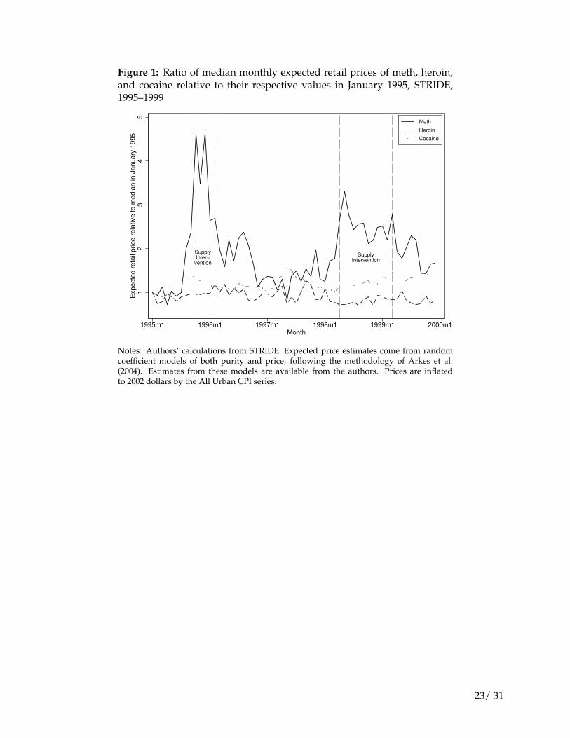
Figure 1: Ratio of median monthly expected retail prices of meth, heroin,and cocaine relative to their respective values in January 1995, STRIDE,1995–1999

SupplyInter−

vention

SupplyIntervention

12

34

5E

xp

ecte

d r

eta

il p

rice

re

lative

to

me

dia

n in

Ja

nu

ary

19

95

1995m1 1996m1 1997m1 1998m1 1999m1 2000m1Month

Meth

Heroin

Cocaine

Notes: Authors’ calculations from STRIDE. Expected price estimates come from randomcoefficient models of both purity and price, following the methodology of Arkes et al.(2004). Estimates from these models are available from the authors. Prices are inflatedto 2002 dollars by the All Urban CPI series.

23/ 31

Figure 2: Estimated own-price elasticities of demand for self-admittedmethamphetamine treatment admissions with respect to the price ofmethamphetamine, 1995–1999

−0

.3−

0.2

−0

.10

.00

.1E

stim

ate

d o

wn

−p

rice

ela

sticity

0 1 2 3 4 5 6Months since meth price shock

Notes: Each plot point represents a coefficient estimate from a single 2SLS regression model.Dashed lines show 90% confidence bounds derived from standard errors that account forheteroskedasticity.

24/ 31

Figure 3: Estimated cross-price elasticities of demand for self-admittedtreatment admissions with respect to the price of methamphetamine, bydrug, 1995–1999

−0.1

0.0

0.1

0.2

0.3

Estim

ate

d c

ross−

price e

lasticity


Panel A: alcohol treatment admissions

−0.1

0.0

0.1

0.2

0.3

Estim

ate

d c

ross−

price e

lasticity


Panel B: heroin treatment admissions

−0.1

0.0

0.1

0.2

0.3

Estim

ate

d c

ross−

price e

lasticity


Panel C: cocaine/crack treatment admissions

−0.1

0.0

0.1

0.2

0.3

Estim

ate

d c

ross−

price e

lasticity


Panel D: marijuana treatment admissions

Notes: Each plot point represents a coefficient estimate from a single 2SLS regression model.Dashed lines show 90% confidence bounds derived from standard errors that account forheteroskedasticity.

25/ 31

Table 1: Selected descriptive statistics, 1995–1999Variables Source N Mean Std. dev. Min. Max.

Proxies for drug useMeth admissions TEDS 2,640 232 599 0 4643Meth admissions, self-referred TEDS 2,640 71 212 0 1848Alcohol admissions TEDS 2,640 2082 2754 34 20522Alcohol admissions, self-referred TEDS 2,640 613 918 0 6567Cocaine/crack admissions TEDS 2,640 1012 1701 4 12158Cocaine/crack admissions, self-referred TEDS 2,640 383 634 0 4125Heroin admissions TEDS 2,640 520 1112 0 6520Heroin admissions, self-referred TEDS 2,640 314 766 0 5464Marijuana admissions TEDS 2,640 927 1162 19 8323Marijuana admissions, self-referred TEDS 2,640 222 275 0 2017

Expected retail prices ($/pure g)Meth price STRIDE 1,398 267 192 36 1483Meth price, imputed STRIDE 2,640 228 95 86 551Crack cocaine price STRIDE 1,605 91 32 43 276Crack cocaine price, imputed STRIDE 2,640 103 24 59 192Powder cocaine price STRIDE 1,520 106 40 47 345Powder cocaine price, imputed STRIDE 2,640 102 23 57 198Heroin price STRIDE 1,011 419 149 176 983Heroin price, imputed STRIDE 2,640 434 65 335 614

ControlsPopulation aged 15–49 years (1,000s) SEER 2,640 2978 3249 309 17975Unemployment rate (%) CPS 2,640 4.57 1.23 1.70 9.00Cigarette tax ($/pack) O&W 2,640 0.33 0.19 0.02 0.93

Notes: Authors’ calculations. The level of variation is state by month. Arizona, the District of Columbia,Indiana, Kentucky, Mississippi, West Virginia, and Wyoming are excluded from the sample because of poordata quality during some or all of the sample period.

26/ 31

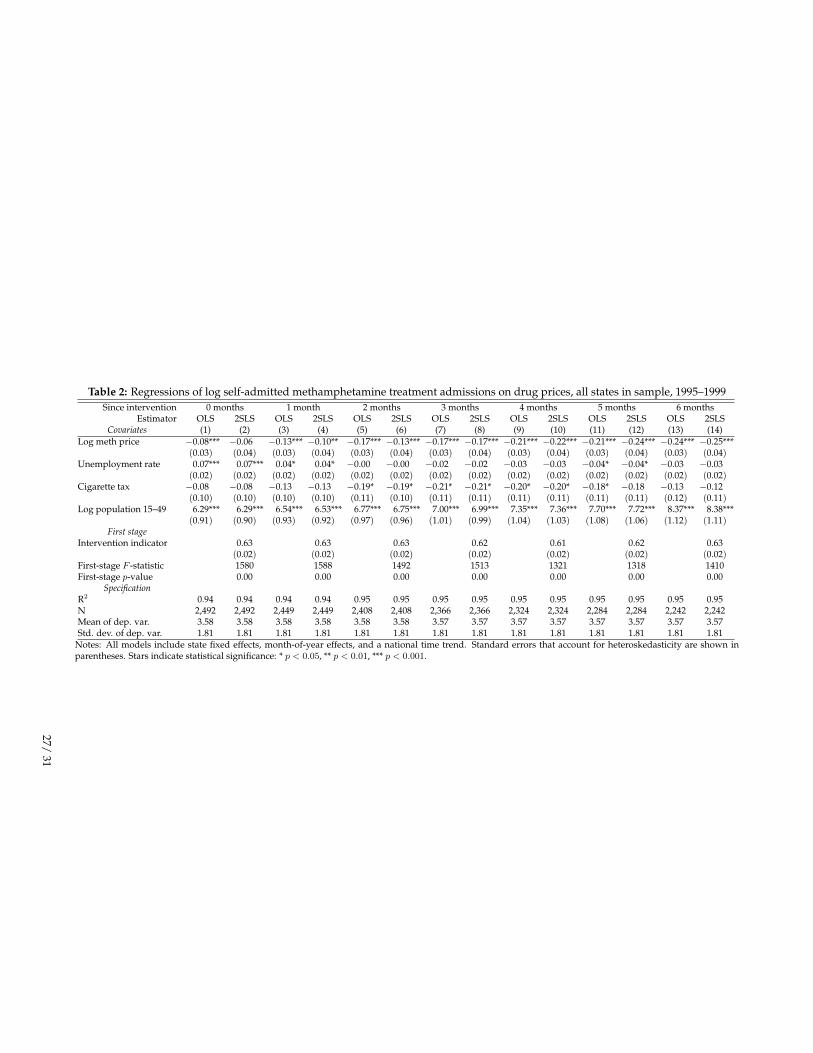
Table 2: Regressions of log self-admitted methamphetamine treatment admissions on drug prices, all states in sample, 1995–1999Since intervention 0 months 1 month 2 months 3 months 4 months 5 months 6 months

Estimator OLS 2SLS OLS 2SLS OLS 2SLS OLS 2SLS OLS 2SLS OLS 2SLS OLS 2SLSCovariates (1) (2) (3) (4) (5) (6) (7) (8) (9) (10) (11) (12) (13) (14)

Log meth price −0.08*** −0.06 −0.13*** −0.10** −0.17*** −0.13*** −0.17*** −0.17*** −0.21*** −0.22*** −0.21*** −0.24*** −0.24*** −0.25***(0.03) (0.04) (0.03) (0.04) (0.03) (0.04) (0.03) (0.04) (0.03) (0.04) (0.03) (0.04) (0.03) (0.04)

Unemployment rate 0.07*** 0.07*** 0.04* 0.04* −0.00 −0.00 −0.02 −0.02 −0.03 −0.03 −0.04* −0.04* −0.03 −0.03(0.02) (0.02) (0.02) (0.02) (0.02) (0.02) (0.02) (0.02) (0.02) (0.02) (0.02) (0.02) (0.02) (0.02)

Cigarette tax −0.08 −0.08 −0.13 −0.13 −0.19* −0.19* −0.21* −0.21* −0.20* −0.20* −0.18* −0.18 −0.13 −0.12(0.10) (0.10) (0.10) (0.10) (0.11) (0.10) (0.11) (0.11) (0.11) (0.11) (0.11) (0.11) (0.12) (0.11)

Log population 15–49 6.29*** 6.29*** 6.54*** 6.53*** 6.77*** 6.75*** 7.00*** 6.99*** 7.35*** 7.36*** 7.70*** 7.72*** 8.37*** 8.38***(0.91) (0.90) (0.93) (0.92) (0.97) (0.96) (1.01) (0.99) (1.04) (1.03) (1.08) (1.06) (1.12) (1.11)

First stageIntervention indicator 0.63 0.63 0.63 0.62 0.61 0.62 0.63

(0.02) (0.02) (0.02) (0.02) (0.02) (0.02) (0.02)First-stage F -statistic 1580 1588 1492 1513 1321 1318 1410First-stage p-value 0.00 0.00 0.00 0.00 0.00 0.00 0.00

SpecificationR2 0.94 0.94 0.94 0.94 0.95 0.95 0.95 0.95 0.95 0.95 0.95 0.95 0.95 0.95N 2,492 2,492 2,449 2,449 2,408 2,408 2,366 2,366 2,324 2,324 2,284 2,284 2,242 2,242Mean of dep. var. 3.58 3.58 3.58 3.58 3.58 3.58 3.57 3.57 3.57 3.57 3.57 3.57 3.57 3.57Std. dev. of dep. var. 1.81 1.81 1.81 1.81 1.81 1.81 1.81 1.81 1.81 1.81 1.81 1.81 1.81 1.81

Notes: All models include state fixed effects, month-of-year effects, and a national time trend. Standard errors that account for heteroskedasticity are shown inparentheses. Stars indicate statistical significance: * p < 0.05, ** p < 0.01, *** p < 0.001.

27/31

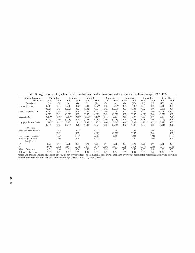
Table 3: Regressions of log self-admitted alcohol treatment admissions on drug prices, all states in sample, 1995–1999Since intervention 0 months 1 month 2 months 3 months 4 months 5 months 6 months


Log meth price 0.01 0.04 0.01 0.06* 0.01 0.07** 0.03 0.07** 0.01 0.06* 0.00 0.05 −0.01 0.03(0.02) (0.03) (0.02) (0.03) (0.02) (0.03) (0.02) (0.03) (0.03) (0.03) (0.02) (0.04) (0.03) (0.04)

Unemployment rate 0.09*** 0.09*** 0.08*** 0.08*** 0.07*** 0.07*** 0.04** 0.04** 0.02 0.02 0.00 0.00 −0.01 −0.02(0.02) (0.02) (0.02) (0.02) (0.02) (0.02) (0.02) (0.02) (0.02) (0.02) (0.02) (0.02) (0.02) (0.02)

Cigarette tax 0.19** 0.19** 0.19** 0.19** 0.18** 0.18** 0.14* 0.13 0.11 0.09 0.09 0.08 0.09 0.08(0.09) (0.09) (0.08) (0.08) (0.08) (0.08) (0.09) (0.08) (0.08) (0.08) (0.08) (0.08) (0.09) (0.09)

Log population 15–49 2.91*** 2.91*** 2.93*** 2.92*** 2.97*** 2.95*** 3.06*** 3.04*** 3.10*** 3.07*** 3.23*** 3.21*** 3.37*** 3.35***(0.75) (0.75) (0.78) (0.78) (0.82) (0.82) (0.85) (0.84) (0.87) (0.87) (0.89) (0.88) (0.91) (0.90)





28/31

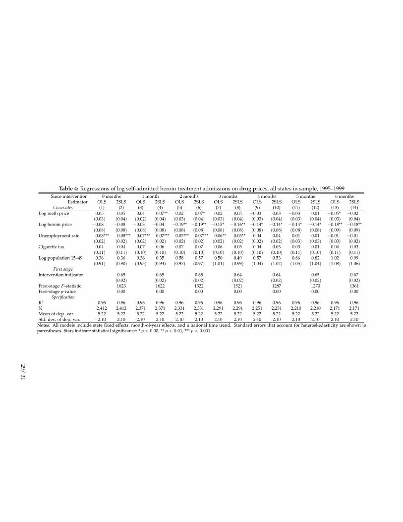
Table 4: Regressions of log self-admitted heroin treatment admissions on drug prices, all states in sample, 1995–1999Since intervention 0 months 1 month 2 months 3 months 4 months 5 months 6 months


Log meth price 0.05 0.05 0.04 0.07** 0.02 0.07* 0.02 0.05 −0.03 0.03 −0.03 0.01 −0.05* −0.02(0.03) (0.04) (0.02) (0.04) (0.03) (0.04) (0.03) (0.04) (0.03) (0.04) (0.03) (0.04) (0.03) (0.04)

Log heroin price −0.08 −0.08 −0.03 −0.04 −0.19** −0.19** −0.15* −0.16** −0.14* −0.14* −0.14* −0.14* −0.18** −0.18**(0.08) (0.08) (0.08) (0.08) (0.08) (0.08) (0.08) (0.08) (0.08) (0.08) (0.08) (0.08) (0.09) (0.09)

Unemployment rate 0.08*** 0.08*** 0.07*** 0.07*** 0.07*** 0.07*** 0.06** 0.05** 0.04 0.04 0.01 0.01 −0.01 −0.01(0.02) (0.02) (0.02) (0.02) (0.02) (0.02) (0.02) (0.02) (0.02) (0.02) (0.03) (0.03) (0.03) (0.02)

Cigarette tax 0.04 0.04 0.07 0.06 0.07 0.07 0.06 0.05 0.04 0.03 0.03 0.01 0.04 0.03(0.11) (0.11) (0.10) (0.10) (0.10) (0.10) (0.10) (0.10) (0.10) (0.10) (0.11) (0.10) (0.11) (0.11)

Log population 15–49 0.36 0.36 0.36 0.35 0.58 0.57 0.50 0.49 0.57 0.53 0.86 0.82 1.02 0.99(0.91) (0.90) (0.95) (0.94) (0.97) (0.97) (1.01) (0.99) (1.04) (1.02) (1.05) (1.04) (1.08) (1.06)





29/31

Table 5: Regressions of log self-admitted crack and powder cocaine treatment admissions on drug prices, all states in sample, 1995–1999Since intervention 0 months 1 month 2 months 3 months 4 months 5 months 6 months


Log meth price −0.00 0.03 0.00 0.05 0.02 0.07** 0.05* 0.07** 0.04 0.06 0.03 0.05 0.02 0.01(0.03) (0.04) (0.02) (0.03) (0.03) (0.03) (0.03) (0.04) (0.03) (0.04) (0.03) (0.04) (0.03) (0.04)

Log crack price −0.09** −0.09** −0.08* −0.08* −0.05 −0.05 −0.09** −0.08** −0.01 −0.01 −0.02 −0.02 −0.01 −0.01(0.04) (0.04) (0.05) (0.05) (0.04) (0.04) (0.04) (0.04) (0.05) (0.05) (0.06) (0.06) (0.05) (0.05)

Log powder price 0.01 −0.00 −0.00 −0.02 −0.05 −0.06 −0.05 −0.06 −0.05 −0.06 −0.06 −0.06 0.02 0.02(0.04) (0.04) (0.04) (0.04) (0.04) (0.04) (0.04) (0.04) (0.04) (0.04) (0.04) (0.05) (0.04) (0.04)

Unemployment rate 0.13*** 0.13*** 0.12*** 0.12*** 0.10*** 0.10*** 0.08*** 0.08*** 0.05** 0.05** 0.02 0.02 −0.01 −0.01(0.02) (0.02) (0.02) (0.02) (0.02) (0.02) (0.02) (0.02) (0.02) (0.02) (0.02) (0.02) (0.02) (0.02)

Cigarette tax −0.00 0.00 0.02 0.01 0.02 0.01 −0.02 −0.02 −0.05 −0.05 −0.08 −0.09 −0.10 −0.10(0.10) (0.10) (0.09) (0.09) (0.10) (0.09) (0.09) (0.09) (0.09) (0.09) (0.09) (0.09) (0.10) (0.10)

Log population 15–49 3.07*** 3.06*** 3.11*** 3.08*** 3.16*** 3.12*** 3.23*** 3.21*** 3.31*** 3.29*** 3.48*** 3.47*** 3.70*** 3.71***(0.84) (0.84) (0.89) (0.88) (0.94) (0.94) (0.97) (0.96) (0.99) (0.98) (1.00) (0.99) (1.03) (1.02)





30/31

Table 6: Regressions of log self-admitted marijuana treatment admissions on drug prices, all states in sample, 1995–1999Since intervention 0 months 1 month 2 months 3 months 4 months 5 months 6 months


Log meth price 0.02 0.03 0.01 0.04 0.02 0.05* 0.03 0.05 0.02 0.04 0.01 0.04 0.00 0.01(0.02) (0.03) (0.02) (0.03) (0.02) (0.03) (0.02) (0.03) (0.03) (0.03) (0.02) (0.03) (0.03) (0.03)

Unemployment rate 0.08*** 0.08*** 0.07*** 0.07*** 0.05** 0.05** 0.02 0.02 −0.00 −0.00 −0.02 −0.02 −0.04** −0.04**(0.02) (0.02) (0.02) (0.02) (0.02) (0.02) (0.02) (0.02) (0.02) (0.02) (0.02) (0.02) (0.02) (0.02)

Cigarette tax 0.27*** 0.27*** 0.27*** 0.27*** 0.25*** 0.24*** 0.19** 0.19** 0.14* 0.13* 0.10 0.10 0.08 0.08(0.09) (0.09) (0.08) (0.08) (0.08) (0.08) (0.08) (0.08) (0.08) (0.08) (0.08) (0.08) (0.09) (0.08)

Log population 15–49 2.14*** 2.14*** 2.22*** 2.21*** 2.30*** 2.29*** 2.43*** 2.42*** 2.53*** 2.52*** 2.67*** 2.65*** 2.75*** 2.75***(0.68) (0.67) (0.71) (0.71) (0.75) (0.75) (0.78) (0.77) (0.81) (0.80) (0.83) (0.82) (0.86) (0.86)





31/31

Identifying Demand Responses to Illegal Drug …economic/RePEc/pdf/tul1312.pdfIdentifying Demand...

Documents

Transcript of Identifying Demand Responses to Illegal Drug …economic/RePEc/pdf/tul1312.pdfIdentifying Demand...