Identifying codes in hereditary classes of graphs andVC-dimension

Nicolas Bousquet1,5, Aurélie Lagoutte ∗2, Zhentao Li †3, Aline Parreau ‡4

and Stéphan Thomassé ∗2

1LIRMM, Université Montpellier 2, France2LIP, UMR 5668 ENS Lyon - CNRS - UCBL - INRIA, Université de Lyon,

France3École Normale Supérieure, Paris, France

4Université de Liege, Belgique5Department of Mathematics and Statistics, McGill University and GERAD,

Montréal, Canada

AbstractAn identifying code of a graph is a subset of its vertices such that every vertex of

the graph is uniquely identified by the set of its neighbours within the code. We showa dichotomy for the size of the smallest identifying code in classes of graphs closedunder induced subgraphs. Our dichotomy is derived from the VC-dimension of theconsidered class C, that is the maximum VC-dimension over the hypergraphs formedby the closed neighbourhoods of elements of C. We show that hereditary classeswith infinite VC-dimension have infinitely many graphs with an identifying code ofsize logarithmic in the number of vertices while classes with finite VC-dimension havea polynomial lower bound.

We then turn to approximation algorithms. We show that Min Id Code (theproblem of finding a smallest identifying code in a given graph from some class C)is log-APX-hard for any hereditary class of infinite VC-dimension. For hereditaryclasses of finite VC-dimension, the only known previous results show that we canapproximate Min Id Code within a constant factor in some particular classes, e.g.line graphs, planar graphs and unit interval graphs. We prove that Min Id Codecan be approximate within a factor 6 for interval graphs. In contrast, we show thatMin Id Code on C4-free bipartite graphs (a class of finite VC-dimension) cannot beapproximated to within a factor of c log(|V |) for some c > 0.

∗Partially supported by ANR Project Stint under Contract ANR-13-BS02-0007.†Partially supported by a FQRNT B3 postdoctoral fellowship program.‡Supported by a FNRS post-doctoral grant at the University of Liège.

1

1 IntroductionLet G = (V,E) be a graph. An identifying code of G is a subset C of vertices of G such that,for each vertex v ∈ V , the set of vertices in C at distance at most 1 from v, is non-emptyand uniquely identifies v. In other words, for each vertex v ∈ V (G), we have N [v]∩C 6= ∅(C is a dominating set) and for each pair u, v ∈ V (G), we have N [u] ∩ C 6= N [v] ∩ C (Cis a separating set), where N [v] denotes the closed neighbourhood of v in G (v and all itsneighbours). We say that a set X of vertices distinguishes u ∈ V (G) from v ∈ V (G) ifN [u] ∩X 6= N [v] ∩X. This concept was introduced in 1998 by Karpovsky, Chakrabartyand Levitin [19] and has applications in various areas such as fault-diagnosis [19], routingin networks [21] or analysis of RNA structures [17]. For a complete survey on these results,the reader is referred to the online bibliography of Lobstein [22].

Two vertices u and v are twins if N [u] = N [v]. The whole vertex set V (G) is anidentifying code if and only if G is twin-free. Since supersets of identifying codes areidentifying, an identifying code exists for G if and only if it is twin-free. A natural problemin the study of identifying codes is to find one of a minimum size. Given a twin-free graphG, the smallest size of an identifying code of G is called the identifying code number of Gand is denoted by γID(G). The problem of determining γID is called the Min Id Codeproblem, and its decision version is NP-complete [8].

Let X ⊆ V . We denote by G[X] the graph induced by the subset of vertices X. Inthis paper, we focus on hereditary classes of graphs, that is classes closed under takinginduced subgraphs. We consider the two following problems: finding good lower boundsand approximation algorithms for the identifying code number.

1.1 Previous work

In the class of all graphs, the best lower bound is γID(G) ≥ log(|V (G)| + 1), since all thevertices of the graphs have distinct non-empty neighbourhood within the code. Moncel [25]characterized all graphs reaching this lower bound. As for approximation algorithms, thegeneral problem Min Id Code is known to be log-APX-hard [20, 21, 30]. In particular,there is no (1 − ε) log(|V |)-approximation algorithm for Min Id Code. The problemMin Id Code remains log-APX-hard even in split graphs, bipartite graphs or co-bipartitegraphs (complement of bipartite graphs) [13].

On the positive side, there always exists a O(log |V (G)|) approximation for Min IdCode [30]. Moreover, even if in the general case Min Id Code is hard to evaluate, thereexist several constant approximation algorithms for restricted classes of graphs, such asplanar graphs [26] or line graphs [14].

For the remainder of this article, n denotes the number of vertices of G. Table 1 givesan overview of the currently known results for some restricted hereditary classes of graphs.The order of magnitude of all lower bounds are best possible (there are infinite families ofgraphs reaching the lower bounds). Min Id Code for line graphs and planar graphs havea polynomial time constant factor approximation algorithm with the best known constantwritten in parenthesis. From this table, we observe two behaviours: a class either

2

1. has a logarithmic lower bound on the size of identifying codes, and Min Id Code islog-APX-hard in this class (for example split, bipartite, co-bipartite graphs), or

2. there is a polynomial lower-bound on γID(G) and a constant factor approximationalgorithm to compute γID(G).

Graph class Lower bound Complexity Approximability ReferencesAll graphs Θ(log(n)) NP-c log-APX-hard [19, 20]Chordal Θ(log(n)) NP-c log-APX-hard [13]

Split graphs Θ(log(n)) NP-c log-APX-hard [13]Bipartite Θ(log(n)) NP-c log-APX-hard [13]

Co-bipartite Θ(log(n)) NP-c log-APX-hard [13]Claw-free Θ(log(n)) NP-c log-APX-hard [13]Interval Θ(n1/2) NP-c open [15]

Unit interval Θ(n) open PTAS [12, 15]Permutation Θ(n1/2) NP-c open [15]Line graphs Θ(n1/2) NP-c APX(4) [14]

Planar Θ(n) NP-c APX(7) [3, 26]

Table 1: Known lower bounds on γID(G) and approximability of γID(G).

1.2 Our results

The aim of this paper is to shed some light on the validity of such a dichotomy for allclasses of graphs using the VC-dimension of the class of graphs.

VC-dimension LetH = (V, E) be a hypergraph. A subset X ⊆ V of vertices is shatteredif for every subset S of X, there is some hyperedge e such that e ∩ X = S. The VC-dimension of H is the size of the largest shattered set of H. We define the VC-dimensionof a graph as the VC-dimension of the closed neighbourhood hypergraph of G (verticesare the vertices of G and hyperedges are the closed neighbourhoods of vertices of G), aclassical way to define the VC-dimension of a graph (see [1, 6]).

By a shattered set of a graph G, we mean a shattered set of the hypergraph of the closedneighbourhoods of G. The VC-dimension of a class of graphs C, denoted by dim(C), is themaximum of the VC-dimension of the graphs over C. If it is unbounded, we say that C hasinfinite VC-dimension.

Dichotomy for lower bounds First we will prove in Section 2 that there is indeed sucha dichotomy on the minimum size of identifying codes: it is always either logarithmic orpolynomial, where the exponent of the polynomial depends on the VC-dimension of the

3

Graph class VC dim IC-lower bound IC-approxGirth ≥ 5 2 Θ(n

12 ) (opt,new) open

Interval 2 Θ(n12 ) (opt) 6 (Thm. 21)

Chordal bipartite 3 Ω(n13 ) (new) open

Unit disk 3 Ω(n13 ) (new) open

C4-free bipartite 2 Θ(n12 ) (opt,new) no c log(n)-approx (Thm. 15)

Undirected path 3 Ω(n13 )(new) open

Table 2: Overview of the results obtained in this paper.

class of graphs. In particular, our theorem provides new lower bounds for graphs of girth atleast 5, chordal bipartite graphs, unit disk graphs and undirected path graphs. Moreover,these bounds are tight for interval graphs and graphs of girth at least 5.

Approximation hardness We then try to extend this dichotomy result for constantfactor approximations. First, we show in Section 3 that Min Id Code is log-APX-hardfor any hereditary class with a logarithmic lower bound. The proof essentially consistsin proving that a hereditary class with infinite VC-dimension contains one of these threeclasses, for which Min Id Code has been shown to be log-APX-hard [13]: the bipartitegraphs, the co-bipartite graphs, or the split graphs. Unfortunately, the dichotomy doesnot extend to approximation since we show in Section 4 that C4-free bipartite graphshave a polynomial lower bound on the size of identifying codes but Min Id Code is notapproximable to within a factor c log n for some c > 0 (under some complexity assumption)in this class. Thus, a constant factor approximation is not always possible in the secondcase.

Approximation algorithm Finally, in Section 5, we conclude the paper with somepositive result when the lower bound is polynomial by proving that there exists a 6-approximation algorithm for interval graphs, a problem left open in [13].

The results obtained in this paper are detailed in Table 2.

2 Dichotomy for lower boundThe following lemma, due to Sauer [27] and Shellah [29] will be useful to prove that thesize of an identifying code cannot be too small if the VC-dimension is bounded. The traceof a set X on Y is X ∩ Y . By extension, the trace of a vertex x on Y is the intersection ofN [x] with Y .

4

Lemma 1 (Sauer’s lemma [27, 29]). Let H = (V, E) be an hypergraph of VC-dimension d.For every set X ⊆ V , the number of (distinct) traces of E on X is at most

d∑i=0

(|X|i

)≤ |X|d + 1.

Let us now prove the main result of this section.

Theorem 2. For every hereditary class of graphs C, either

1. for every k ∈ N, there exists a graph Gk ∈ C with more than 2k − 1 vertices and anidentifying code of size 2k, or

2. there exists ε > 0 such that no twin-free graph G ∈ C with n vertices has an identifyingcode of size smaller than nε.

Proof. Let C be an hereditary class of graphs. The class C either has finite or infinite VC-dimension. First, suppose that C has infinite VC-dimension. We will show that C satisfiesthe first conclusion. By definition of infinite VC-dimension, there is a graph Hk ∈ C withVC-dimension k for each k. So there exists a set of vertices X of size k of Hk which isshattered. Let Y be a set of 2k − 1 vertices whose closed neighbourhoods have all possibletraces on X except the empty set, meaning that for every X ′ ⊆ X, add a vertex y in Ysuch that N [y] ∩X = X ′. Choose Y so that |X ∩ Y | is maximized. Let Gk = Hk[X ∪ Y ].The graph Gk has at least 2k− 1 vertices since |Y | = 2k− 1. By choice of Y , X dominatesX ∪ Y and X distinguishes every pair of vertices of Y . By maximality of |X ∩ Y |, X alsodistinguishes every vertex in X from every vertex in Y (otherwise a vertex of Y wouldhave the same neighbourhood in X as a vertex x ∈ X and thus can be replaced by x,contradicting the maximality of |X ∩Y |). For each x ∈ X, the vertex yx ∈ Y whose closedneighbourhood intersects X in exactly x distinguishes x from all vertices in X − x. SoX ∪ yx|x ∈ X is an identifying code of size at most 2k, as required.

Now suppose that the VC-dimension of C is bounded by d. For any identifying codeC of a twin-free graph G ∈ C, the traces of vertices of G on C are different. Hence, byLemma 1, n ≤ ∑d

i=0

(|C|i

)≤ |C|d + 1. Therefore, |C| ≥ (n − 1)

1d , proving that C satisfies

the second claim.

The proof gives in fact the lower bound γID(G) ∈ Ω(n1

dim(C) ) for the second item. So ifwe can bound the VC-dimension of the class, then we immediately obtain lower bounds onthe size of identifying codes. Lemma 3 provides such bounds for several classes of graphs.

Let us give some definitions. The girth of a graph is the length of a shortest cycle.A chordal bipartite graph is a bipartite graph without induced cycle of length at least 6.A unit disk graph is a graph of intersection of unit disks in the plane. An interval graphis a graph of intersection of segments on a line. An undirected path graph is a graph ofvertex-intersection of paths in an undirected tree (i.e. two vertices are adjacent if theircorresponding paths have at least one vertex in common).

5

x1 x2

x3

Figure 1: The set x1, x2, x3 is shatteredin this chordal bipartite graph.

Figure 2: A set of three vertices shat-tered by disks in the plane.

Lemma 3. The following upper bounds hold and are tight:

• The VC-dimension of graphs of girth at least 5 is at most 2.

• The VC-dimension of chordal bipartite graphs is at most 3.

• The VC-dimension of unit disk graphs is at most 3.

• The VC-dimension of interval graphs is at most 2.

• The VC-dimension of undirected path graphs is at most 3.

Proof.

• Let G be a graph of girth at least 5. Assume by contradiction that a set x1, x2, x3 ofthree vertices is shattered. Since the girth is at least 5, x1x2x3 is not a clique. We mayassume without loss of generality that x1 and x2 are not adjacent. Since x1, x2, x3is shattered, there is a vertex y1 adjacent to both x1 and x2 and not x3 (one closedneighbourhood must have trace x1, x2 on x1, x2, x3) and a vertex y2 adjacent tox1, x2, x3 (one closed neighbourhood must have trace x1, x2, x3). Note that bothy1 and y2 are distinct from x1 and x2 since x1 and x2 are not adjacent. Moreover y1and y2 are distinct since they do not have the same neighbourhood in x1, x2, x3.So x1y1x2y2x1 is a cycle of length 4, a contradiction with the girth assumption.This bound is tight, for instance with the path on six vertices.

• Let G = (A ∪ B,E) be a chordal bipartite graph. Assume by contradiction thatx1, x2, x3, x4 is a shattered set of four vertices. Since there is a vertex whose closedneighbourhood contains the whole set of vertices, it means that at least three vertices,say x1, x2, x3 are on the same side of the bipartite graph. Since a subset of a shatteredset is shattered, x1, x2, x3 is shattered. Thus there is a vertex incident to x1, x2and not x3, a vertex incident to x1, x3 and not x2, and a vertex incident to x2, x3 andnot x1. It provides an induced cycle of length 6, a contradiction.Moreover the bound is tight, see Figure 1.

6

P1

P2 P3

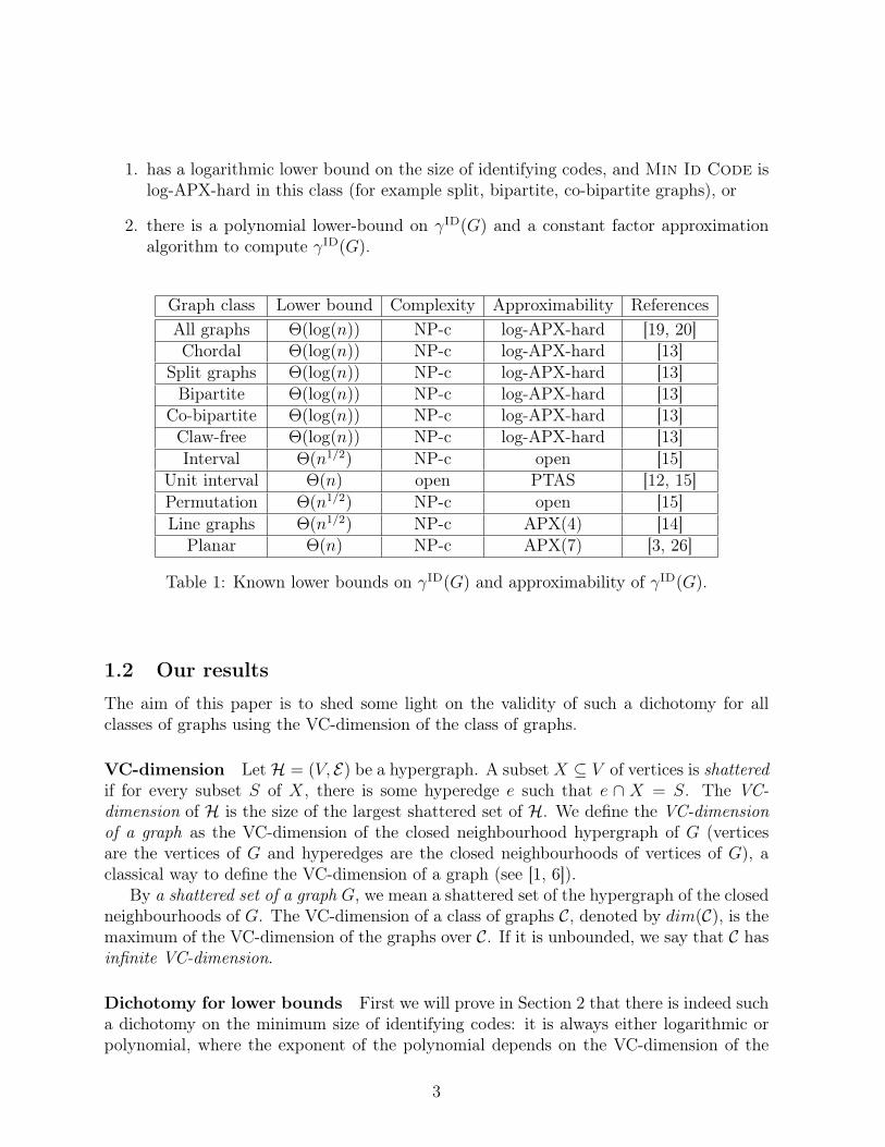
Figure 3: Paths P1, P2, P3 are shattered by the eight points which are paths of length 0.

• Let G be a unit disk graph. Let us rephrase the adjacency and shattering conditionsin this class: let x1 and x2 be any two vertices of a unit disk graph and denote by c1and c2 their respective centers in a representation of the unit disk graph in the plane.The vertices x1 and x2 are adjacent if and only if c1 and c2 are at distance at most 2.Thus if a set of unit disks is shattered then for every subset of centers, there exists apoint at distance at most 2 from these centers and more than 2 from the others. Inother words, there exist points in all possible intersections of balls of radius 2.A classical result ensures that the VC-dimension of a hypergraph whose hyperedgescan be represented as a set of disks in the plane (and vertices as points of the plane)has VC-dimension at most 3 (see [24] for instance). Thus unit disk graphs haveVC-dimension at most 3, and the bound can be reached (see Figure 2).

• Let G be an interval graph. Assume by contradiction that there is a shattered setI1, I2, I3 of G. Assume that I1 starts before I2 and that I2 starts before I3. Sincethere is an interval J intersecting both I1 and I3 but not I2, J must start afterI2 and thus I1 contains I2. Then there is no interval intersecting I2 but not I1, acontradiction. Thus interval graphs have VC-dimension at most 2, and the bound isagain reached with the path on six vertices.

• Let P = P1, P2, P3, P4 be a shattered set of four paths of a tree T . Assume firstthat P2, P3, P4 all intersect P1 and consider the restriction of T to P1, which is in factan interval graph. To ensure all possible intersections with P1, the set P2, P3, P4 isa shattered set of size three in an interval graph, a contradiction.

Thus at least one path, say P2, does not intersect P1 and lies in a connected com-ponent C of the forest F = T \ P1. If P3 does not intersect C, then there is nopath intersecting both P2 and P3 but not P1. Thus P3 intersects C. If moreover P3

intersects P1, then no path can intersect both P1 and P2 but not P3. Thus P3 isalso included in C. Let P be a path intersecting P1, P2 and P3. Assume first that Pintersects the three paths in the order P1, P2 and P3 (the case P1, P3, P2) is the same.Then no path can intersect P1 and P3 without intersecting P2. Assume now that Pintersects the three paths in the order P2, P1, P3. Similarly, no path can intersectP2 and P3 without intersecting P1. Hence the path P cannot exist, a contradiction.Finally the bound of 3 can be reached, as shown in Figure 3.

7

Lemma 3 and Theorem 2 imply new lower bounds for many classes: Ω(n12 ) for graphs

with girth at least 5, Ω(n13 ) for chordal bipartite graphs, Ω(n

13 ) for unit-disk graphs, Ω(n

12 )

for interval graphs, Ω(n13 ) for permutation graphs, and Ω(n

13 ) for undirected path graphs.

The exponent given by Theorem 2 is sharp for several classes of graphs. Indeed, Foucaudet al. [15] proved that there are infintely many interval graphs with identifying codes ofsize Θ(n1/2). The bound is also tight for C4-free bipartite graphs (which have girth at least5): the following construction is a C4-free bipartite graphs with an identifying code of sizeΘ(n

12 ). Let G = (X ∪ Y,E) be a bipartite graph where Y has size n, X has size n(n−1)

2,

and edges satisfy the following rule: for every pair u, v of vertices of Y , there is exactly onevertex of X adjacent to both u and v. The graph G does not contain any triangle (sinceit is bipartite) nor C4 (since neighbourhoods intersect on at most one vertex). One caneasily check that the set Y is an identifying code of the graph. Indeed vertices of X areadjacent to precisely two neighbours on Y and vertices of Y have precisely one neighbouron Y in their closed neighbourhood. Finally, it is also sharp for the class of all graphs ofVC-dimension at most d. Indeed, consider the bipartite graph made with a stable set A ofsize d and a stable set B of size

∑di=2

(di

)representing all the subsets of A of size at least 2.

Each vertex of B is adjacent to the vertices of A corresponding to its subset. This graphhas VC-dimension d and the set A is an identifying code of size of order n1/d.

Nevertheless, the bounds given by Theorem 2 are not necessarily tight. For instance,permutations graphs can have VC-dimension 3 but Foucaud et al. [15] recently provedthat the exact lower bound is Ω(n

12 ).

Note that a similar bound can be obtained for identifying codes in hypergraphs wherewe want to distinguish all the hyperedges with a minimal subset of vertices. Such a problemgeneralizes identifying codes and is known under the name of test covering or discriminatingcodes (see Section 4).

3 Inapproximability in infinite VC-dimensionGiven a minimization problem P and a function f : N → N, a factor f approximationalgorithm (also called an f -approximation) is an algorithm that outputs a solution of valueat most f(n) · OPTI for every instance I of P of size n, where OPTI is the value of anoptimal solution of I. log-APX is a class of problems consisting of all problems that admita logarithmic factor polynomial time approximation algorithm. We use the AP-reductionsintroduced in [9] which have now become standard. Its definition restricted minimizationproblems is defined as follows:

Definition 4 ([4]). Let P and Q be two minimization problems. An AP-reduction fromP to Q is a triple (f, g, α) where

1. α is a constant,

2. f maps pairs consisting of an instance of P and a constant r > 1 to instances of Q,and

8

3. g maps triples consisting of a constant r > 1, an instance IP of P and a solution tof(IP , r) to a solution of IP

in such a way that

1. f(IP , r) has a solution if IP does,

2. f(·, r) and g(·, ·, r) are computable in polynomial time for all fixed r, and

3. if f(IP , r) ≤ r ·OPT (f(IP , r)) then g(f(IP , r), r, SOLQ) ≤ (1 +α(r− 1)) ·OPT (IP ).

A problem Q is log-APX-hard if any problem P in log-APX can be reduced to Q byan AP-reduction.

Theorem 5 ([9]). Any optimization problem P that is log-APX-hard with respect to AP-reduction is NP-hard to approximate within a factor c · log(n) where n is the size of theinput, for some constant c > 0.

We show that Min Id Code is log-APX-hard for classes with infinite VC-dimension.To prove this result, we will prove that a class with infinite VC-dimension contains eitherall the bipartite graphs, or all the co-bipartite graphs or all the split graphs. Since theproblem Min Id Code is log-APX-hard in these three classes (see [13]), it implies that itis log-APX-hard for all classes with infinite VC-dimension.

Theorem 6. Let C be an hereditary class. If C has infinite VC-dimension, then C mustcontain either all the bipartite graphs, or all the co-bipartite graphs or all the split graphs.

Note that this result implies the first part of Theorem 2. We say that a bipartite graphH = (A ∪ B,E) is a bipartisation of G if removing all edges in A and in B in G yields Hfor some partition A,B of V (G).

Lemma 7. For any hereditary class C of graphs with infinite VC-dimension and any bi-partite graph H, C contains a graph G whose bipartisation is H.

Proof. Let H = (A ∪ B,E) be a bipartite graph with |B| ≤ |A| = k. Since C hasinfinite VC-dimension, it contains a graph G with a shattered set S of size (at least)` = k + dlog(2k)e. Let A′ be the first k vertices in S, and let us number Y1, . . . , Y2k some2k distinct subsets of S \ A′ (they exists since |S \ A′| = dlog(2k)e).

By definition of a shattered set, for each i ∈ 1, . . . 2k and for each X ⊆ A′ thereis a vertex xi of G such that N [xi] ∩ S = X ∪ Yi. Thus there are 2k vertices of Gwhose closed neighbourhoods intersect A′ in exactly X. Hence there are at least k suchvertices in V (G) \ A′. Label the vertices of A′ by vertices in A, i.e. choose an arbitrarybijection between A and A′. Now for each b ∈ B, choosing X = N(b) gives k vertices inV (G) \ A′ whose closed neighbourhoods intersect A′ in exactly N(b). So we can chooseone "representative" for each b so that all the selected vertices are distinct (since |B| ≤ k).

9

Note that we need k vertices in V \ A′ since up to |B| vertices of B may have the sameneighbourhood in A.

Since C is closed under taking induced subgraphs, the subgraph of G induced by A′ andthe set B′ of all chosen vertices is in C. The bipartisation of this graph is H, as required.

Next we show that we can further restrict H ′ and now require both sides of H ′ to bestable sets or cliques. For a bipartite graph H = (A ∪ B,E), write H1,0 for the graphobtained from H by adding a clique on A, H0,1 the graph obtained from H by adding aclique on B and H1,1 the graph obtained from H by adding a clique on both A and B. Wealso write sometimes H0,0 for H. We show that, for each bipartite graph H, C containsone of these four graphs. To do so, we need the classical theorem of Erdős and Hajnal [10]as well as its bipartite version by Erdős, Hajnal and Pach [11].

Theorem 8 (Erdős, Hajnal [10]). For every graph H, there exists a constant c(H) suchthat all graphs on n vertices contain either H as an induced subgraph, a stable set of sizeat least 2c(H)

√2 logn or a clique of size at least 2c(H)

√2 logn.

Theorem 9 (Erdős, Hajnal, Pach [11]). Let H be a bipartite graph with vertex classes U1

and U2, (k = |U1| ≤ |U2| = `) and let n > `k+1. Then in any bipartite graph G with vertexclasses V1 and V2 (|V1| = |V2| = n) which contains no two subsets U1 ⊆ V1, U2 ⊆ V2 thatinduce an isomorphic copy of H, there exist V ′1 ⊆ V1 and V ′2 ⊆ V2 of size

⌊(n`

) 1k

⌋such that

either all edges between V ′1 and V ′2 belong to G or none of them does.

We continue with the following technical lemmas:

Lemma 10. For n large enough, there exists a bipartite graph G0 = (A ∪ B,E0) with2n vertices (|A| = |B| = n) such that there is no complete nor empty bipartite graphsG0[A

′ ∪B′] with A′ ⊆ A and B′ ⊆ B and |A′| = |B′| = b2 log nc.

Proof. Let us show its existence with a probabilistic argument. Let A and B be twostable sets each of size n and for every a ∈ A, b ∈ B, put the edge ab with probability 1

2.

Given two subsets A′ ⊆ A, B′ ⊆ B with |A′| = |B′| = b2 log nc, the probability that A′∪B′induces a complete bipartite graph is

(12

)b2 lognc2 . The same probability holds for A′ ∪ B′inducing an empty bipartite graph. Thus the probability that there exists a complete orempty bipartite graph with each part of size 2 log n is at most

(n

b2 log nc

)22

2b2 lognc2≤(

n · eb2 log nc

)2·b2 lognc

· 2

2b2 lognc2= 2−4 logn·log logn+O(logn)

using the inequality (n

l

)≤ nl

l!≤(n · e

l

)l10

This probability is strictly less than 1 for n large enough, so there exists a graphG0 = (A ∪B,E0) for which the event does not occur.

Lemma 11. Let C be an hereditary class with infinite VC-dimension. For any bipartitegraph H = (H` ∪Hr, E), one of the four graphs H0,0, H1,0, H0,1 or H1,1 is in C.

Proof. Suppose by contradiction that Lemma 11 is false for H with |H`| ≤ |Hr| = k. Letc(H) be the constant from Theorem 8 and pick n large enough so that 2

c(H)k

√2 logn > kk+1,

and (2c(H)k

√2 logn)/k

1k > 2 log n and n satisfies the condition of Lemma 10. Let G0 be a

bipartite graph as in Lemma 10, i.e. G0 has n vertices on both sides and does not containa complete or an empty bipartite graph with 2 log n vertices on each side. By Lemma 7, Ccontains a graph G whose bipartisation is G0. Let A,B certify this bipartisation.

Since G contains no copy of H0,0, neither does G[A]. So by Theorem 8, G[A] containsa clique or stable set A′ of size at least n′ = 2c(H)

√2 logn. Similarly, G[B] also contains a

clique or stable set B′ of this size. Assume without loss of generality that in both cases,A′ and B′ induce stable sets. By assumption, the bipartisation of G[A′ ∪ B′] contains nocopy of H0,0 (since the class C is closed under induced subgraphs). So by Theorem 9 andsince n′ > kk+1, the bipartisation of G[A′ ∪ B′] contains a complete bipartite graph or anempty bipartite graph where each bipartition has size(

n′

k

) 1k

=2

c(H)k

√2 logn

k1k

> 2 log n

which is a contradiction to G0 having no such subgraph.

Proof of Theorem 6. Let Hn be the disjoint union of every bipartite graphs of size atmost n. For every n, Lemma 11 ensures that Han,bn

n is in C (for some an, bn ∈ 0, 1) andhence there exist a, b ∈ 0, 1 for which Ha,b

n is in C for infinitely many values of n.If a = b = 0, all bipartite graphs are in C; if a 6= b, all split graphs are in C and if

a = b = 1, all co-bipartite graphs are in C: indeed let Ha,b be a bipartite graph on nvertices (resp. split graph, co-bipartite graph, depending on the value of a and b). Thenthere exists n′ ≥ n such that Ha,b

n′ is in C. But Ha,b is an induced subgraph of Hn′ so Ha,b

is an induced subgraph of Ha,bn′ . The theorem follows.

Foucaud [13] proved that Min Id Code is log-APX-hard for bipartite graphs, splitgraphs and co-bipartite graphs. So the following is a direct corollary of Theorem 6.

Corollary 12. Min Id Code is log-APX-hard when the input graph is restricted to anhereditary class of graphs with infinite VC-dimension.

4 Inapproximability for C4-free bipartite graphsIn this section, we examine the complexity of approximating Min Id Code in classes offinite VC-dimension. Previous results suggest that all these classes may have a constant

11

factor approximation algorithm : this is the case for line graphs [14], planar graphs [26] orunit interval graphs (since any solution has size at least n

2) for instance.

However, we show that this intuition is false: the class C of C4-free bipartite graphs(whose VC-dimension is bounded by 2) does not admit such an approximation algorithm.In fact, Min Id Code in C is hard to approximate to within a c log n factor (for somec > 0) in polynomial time, unless NP ⊆ ZTIME(nO(log logn)).

Observation 13. The class of C4-free bipartite graphs has VC-dimension at most 2.

Proof. Let G be a C4-free bipartite graph. Then it has no triangle and no C4, so we canapply the result of Lemma 3 for graphs of girth at least 5.

We provide a polynomial time gap preserving reduction (in fact, an AP-reduction) fromthe following minimization problem:

Problem 14. Set cover with intersection 1 (Set Cover1)Instance: A set X and a family S of subsets of X where any two sets in S intersect in atmost one element.Solution: A subset S ′ of sets in S whose union contain X.Measure: The size of S ′.

Anil Kumar, Arya and Hariharan [2] have shown that this problem cannot be ap-proximated to within a c log n factor (for some c > 0) in polynomial time, unless NP ⊆ZTIME(nO(log logn)).

Theorem 15. Min Id Code with input restricted to C4-free bipartite graphs cannot beapproximated to within a c log n factor (for some c > 0) in polynomial time, unless NP ⊆ZTIME(nO(log logn)) where n is the size of the input.

To give a flavour of our reduction from Set Cover1 to Min Id Code, we first give aneasier reduction to the Discriminating code problem [7]. The Discriminating codeis often a way to design reductions which gives an overview of most complicated ones forMin Id Code : indeed a discriminating code consists in identifying vertices of a set Xusing vertices of a set Y .

Problem 16. Discriminating codeInstance: A bipartite graph G = (X ∪ Y,E).Solution: A subset Y ′ of Y which dominates X and such that for every pair of verticesx1, x2 of X, N [x1] ∩ Y ′ 6= N [x2] ∩ Y ′. Such a set is called a discriminating code.Measure: The size of Y ′.

Lemma 17. Discriminating code with input restricted to C4-free bipartite graphs can-not be approximated to within a c log n factor (for some c > 0) in polynomial time, unlessNP ⊆ ZTIME(nO(log logn)).

12

Proof. Let ISC = (X,S) be an instance of Set Cover1. The proof is decomposed intofive steps: construct an instance IDC of discriminating code that has polynomial size in|ISC |; check that this instance is indeed a C4-free bipartite graph; for every solution of ISC ,construct a solution of IDC ; and vice-versa; finally check that if the solution of IDC is nottoo big with respect to the optimal one, then so is the solution of ISC .

Construct the instance of Discriminating Code Let G = (X ∪ S,E) be themembership bipartite graph of the instance ISC , that is to say that for every x ∈ X, s ∈ S,there is an edge xs ∈ E if and only if x ∈ s. In the following, n denotes the size of Xand we assume that n ≥ 2 and that no s ∈ S is connected to all of X (meaning that theoptimal solution to ISC has size at least 2). Note that in the other case, we can computethe optimal solution in polynomial time. Moreover, we assume that for every x ∈ X,there exists s ∈ S such that x belong to s, otherwise there is no solution. The followingconstruction is illustrated on Figure 4. Let G1, . . . , G` be ` = 2n2 − 1 disjoint copies of G.Denote by Xi∪Si the i-th copy of X∪S. Let X ′1 and X ′2 be copies of X. For each x′′ ∈ X ′2,add an edge between x′′ and its copy x′ in X ′1, and add edges between x′′ and its copies inall Gi for i ≤ `. In other words, G[Xi ∪X ′2] induces a matching for every i. Let GDC bethis bipartite graph with parts XDC = X1 ∪ ... ∪ X` ∪ X ′1 and YDC = S1 ∪ ... ∪ S` ∪ X ′2.Clearly, the size of IDC is polynomial in n an thus in the size of ISC .

Check that the instance is C4-free First note that the initial graph G is C4-free.Indeed every C4 must have two vertices in S and two vertices in C, a contradiction sincethe neighbourhoods of two vertices of S intersect on at most one vertex. Further, thegraph GDC is C4-free. Indeed, no C4 can contain two vertices of S1 ∪ · · · ∪ Sl since anyvertex s ∈ Si only has neighbours in Xi, and GDC [Xi∪Si] is a copy of the C4-free graph G.Moreover, two vertices x′′ ∈ X ′2 and s ∈ Si have at most one common neighbour xi ∈ Xi,the copy of x′′. Finally, each pair of vertices of X ′2 have disjoint neighbourhoods. Thus novertex can be part of a C4.

Transforming a solution of ISC into a solution of IDC Let D be a set cover of Sof size SOLSC . Construct C as the union of ` copies of D (one for each Gi), and finallyadd X ′2. Then C is dominating XDC since X ′2 is, moreover C is separating all the pair ofvertices of XDC . Indeed, two vertices xi, yj inherited from two different elements x, y ∈ Xare separated by x′′ ∈ X ′2, the copy of x in X ′2. Two vertices xi ∈ Xi, xj ∈ Xj with i 6= j,or two vertices xi ∈ Xi, x

′ ∈ X ′1 inherited from the same element x ∈ X are separatedby a neighbour si ∈ Si of xi, where si is the i-th copy of an element s ∈ D containing x.Consequently, C is indeed a discriminating code. For later use, observe that if D is theoptimal solution of Set Cover1 of size OPTSC , we can derive OPTDC ≤ n+ ` ·OPTSC .

Transforming a solution of IDC into a solution of ISC Let C be a solution of IDCof size SOLDC . We construct a set cover candidate D1 = S1 ∩ C. Every vertex x1 ∈ X1

is dominated and separated from its copy x′ in X ′1, and x′′ ∈ X ′2 cannot achieve this goal,

13

X1 S1

X2 S2

X′1 X′

2

. . . . . .

Figure 4: Construction of the proof of Lemma 17.

thus there exists s ∈ S1 ∩ C which is linked to x1. Thus D1 is a set cover. The same canbe done for each i ≤ `, and we choose D as the minimum size such constructed set cover.For later use, observe that X ′2 ⊆ C since X ′1 is dominated. Consequently if SOLSC is thesize of D, we have |X ′2|+ ` · SOLSC ≤ SOLDC or equivalently SOLSC ≤ SOLDC−n

`.

Concluding on the size of the solutions Now suppose that we can obtain a solutionSOLDC of Discriminating Code satisfying SOLDC ≤ r ·OPTDC for some value r. Theabove discussion gives

SOLSC ≤SOLDC − n

`≤ r ·OPTDC − n

`≤ r(n+ ` ·OPTSC)− n

`≤ 2r ·OPTSC

In particular if r = c′ log n for some well-chosen constant c′, we obtain a contradictionwith Set Cover1 approximation hardness.

Let us now adapt this reduction into a reduction to identifying codes.

Proof of Theorem 15. Let ISC be an instance of Set Cover1.

Construct the instance of Min Id Code First construct the same graph GDC asin the proof of Lemma 17. Now for identifying codes, we need to identify vertices in bothsides and not only on the side of XDC . For that, we add to GDC a set Z = z1, . . . , z2n2in part XDC . We have to be careful when we connect the vertices of Z to the vertices ofthe graph since we do not want to create a C4. We aim at choosing edges between Z andS1 ∪ ...∪ S` such that each vertex s ∈ S1 ∪ ...∪ S` is adjacent to exactly two vertices of Z,and no two vertices s, s′ ∈ Si share a neighbour in Z. The following claim (whose proof ispostponed at the end of the section) reaches the goal:

14

Claim 18. There exists a numbering of the vertices in S1 ∪ ... ∪ S` such that:

• Each vertex s ∈ S1 ∪ ... ∪ S` is numbered si,j with i < j ∈ 1, . . . , 2n2, where thepair i, j is distinct for every vertex.

• Two vertices sj,k and sj′,k′ cannot both belong to the same set Si if one of j, k is equalto one of j′, k′.

Using the numbering of the claim, we just have to add the edges zksk,l and zlsk,l forevery k, l ∈ 1, . . . , 2n2. Note that every vertex of Si is connected to precisely two verticesof Z, and that every vertex z ∈ Z has at most one neighbour in each Si. Let GIC be thisnew graph. It has polynomial size in n.

Check that the instance is C4-free Since we only add edges from Z ⊂ XDC toS1∪· · ·∪S` ⊂ YDC , the graph is indeed bipartite. Since GDC was C4-free, any hypotheticalC4 must intersect Z, say in zk ∈ Z. zk share with any zl ∈ Z at most one common neighboursk,l, so the C4 must intersect Xi for some i, or X ′1. On the one hand, vertices in X ′1 havedegree one. On the other hand, xi only has neighbours in Si, and zk has one only neighbourin each Si, so they cannot be in the same C4.

Transforming a solution of ISC into a solution of IIC A set C containing X1∪X ′2∪Zis a good candidate to be an identifying code because it has the following properties:

• For every zk ∈ Z, zk is identified by zk being the only vertex of Z ∩N [zk] ∩ C.

• For every copy x′′ ∈ X ′2 of an element x ∈ X, x′′ is dominated by x”, x1 in C awhere x1 ∈ X1 is the copy of x. Thus it is separated from all the other vertices exceptmaybe x1.

• For every sk,l ∈ S1 ∪ . . . ∪ S`, sk,l is identified by zk, zl.

• For every x′ ∈ X ′1, x′ is dominated by x′′ ∈ X ′2.

• For every xi ∈ Xi, xi is dominated by x′′ ∈ X ′2Thus C is a dominating set, and the only sets of vertices that may be not separated

are of the form x′ ∪ x2, . . . , x` and x”, x1 for any element x ∈ X.Let D be a set cover of the initial instance and D1, ..., D` be the respective copies in the

graphs Gi. Then C = D1∪...∪D`∪X1∪X ′2∪Z is an identifying code of GIC . Indeed, everyvertex xi is separated from x′, x” and xj (i 6= j) by the element of Si that covers it in the setcover Di. Hence any solution for Set Cover1 of size SOLSC gives a solution for Min IdCode of size SOLIC = ` ·SOLSC +2n+2n2. In particular OPTIC ≤ ` ·OPTSC +2n+2n2.

15

Transforming a solution of IIC into a solution of ISC Let C be an identifying codeof GIC . We define Di = C ∩ Si as a set cover candidate. Unfortunately, Di may not be aset cover, in which case we iteratively modify C until all Di meet the condition. If Di isnot a set cover of Xi, then there is a vertex xi not covered. This vertex must be separatedwith its copy x′ in X ′1, hence xi (case 1) or x′ (case 2) must belong to C (if both occur,case 1 has priority on case 2). Then choose any neighbour s ∈ Si of xi, add this vertex toC and remove xi (in case 1) or x′ (in case 2). We thus get a new set C ′ and claim thatC ′ ∪ Z ∪X1 ∪X ′2 is an identifying code. Thanks to the above discussion, we just have toshow that the sets x′ ∪ x2, . . . , x` and x”, x1 are separated.

Observe first that xi is now separated from x′ and from xj by s for j 6= i. Moreover,since C was separating xj1 from xj2 for j1, j2 6= i, then C ′ still does (because nothingchanged in their neighbourhood). We also have C ′ that separates x′ from xj for j 6= i: thevertex separating those two vertices was not xi, so in case 1 it still belongs to C ′. In case2, we have removed x′ but then xi was not in C, and C was separating xi and xj so thereexists a vertex in (N [xj] \ x′) ∩ C, and this vertex separates xj from x′ in C ′. Finally,C ′ still separates x1 from x” since these two vertices cannot be separated by xi nor x′.

Hence we can assume that all the sets C ′ ∩ Si are set covers where C ′ has size at most|C| + 2n + 2n2. Since there are at most |C| vertices of C ′ which are in S1 ∪ . . . ∪ S`, Itmeans that an identifying code with |C| = SOLIC vertices of GIC gives a solution of setcover with SOLSC ≤ SOLIC

`vertices.

Concluding on the size of the solutions Assume now that SOLIC ≤ r · OPTIC forsome value r, then:

SOLSC ≤SOLIC

`≤ r ·OPTIC

`≤ r((2n2 − 1)OPTSC + 2n+ 2n2)

2n2 − 1≤ 2r ·OPTSC

As before for discriminating codes, it achieves the proof of Theorem 15.

An edge colouring of a graph with k colours is a function c : E → 1, . . . , k such thatno two edges sharing an endpoint are given the same colour, that is c(uv) 6= c(uv′) forevery pair of edges uv, uv′.

Proof of Claim 18. We first need to convince ourselves that |S| ≤ n2 in the instance(X,S) of Set Cover1. Indeed every pair of elements of X appears in at most one s ∈ S,thus |S| ≤ n(n+1)

2≤ n2 (one for each pair plus n additional singletons).

Now the idea of the proof is the following: we will represent our problem using a cliqueon 2n2 vertices. The vertices of the clique represent vertices of Z and edges of the cliquerepresent vertices of S1 ∪ · · · ∪ S`.

The edges ofK2n2 can be partitioned into 2n2−1 perfect matchings, or equivalently thereexists an edge colouring c of K2n2 with 2n2− 1 colours such that each colour class containn2 edges. Then label the vertices by z1, . . . , z2n2 and create a set S ′ = S ′1 ∪ · · · ∪ S ′2n2−1

16

of elements sj,k with j, k ∈ N according to the following rule:

S ′i = sj,k|c(zjzk) = i for every i ∈ 1, . . . 2n2 − 1

Observe that |S ′i| = n2. Since a colour class is a matching, the indices of every pair ofedges in a same colour class are pairwise distinct. In other words, there cannot be twovertices sj,k and sj′,k′ in the same set S ′i if one of j, k is equal to one of j′, k′. Now choosearbitrarily |S| ≤ n2 vertices in S ′i to form Si.

5 Constant approximation algorithm for interval graphsWe now focus on the class of interval graphs and provide a constant factor approxima-tion algorithm for Min Id Code via a linear programming approach. More precisely weshow that Min Id Code has a 6-approximation algorithm. The existence of a constantapproximation algorithm was left open in [13].

Let us recall that an interval graph is a graph which can be represented as an intersectionof segments in the real line. We put an arbitrary order on the real line. The begin date ofan interval x is the first point p of the real line (in the order) such that p ∈ x. The enddate of x is the last point which is in x. By abuse of notations, we will denote by v boththe vertex of the graph and the interval in the representation on the real line. Note thatthere exist many representations as intersections of segments for a same interval graphs,we choose arbitrarily one of them which can be found in linear time [5].

Let G be an interval graph together with an interval representation. We denote itsvertex set by 1, . . . , n and U 5 U ′ stands for the symmetric difference of U and U ′ forU,U ′ ⊆ V . Let us express Min Id Code in terms of an integer program P , where xi isthe decision variable corresponding to vertex i:

Integer program P

Objective function: min∑i∈V

xi

Separation constraint:∑

i∈N [j]5N [k]

xi ≥ 1 ∀j 6= k ∈ V

Domination constraint:∑i∈N [j]

xi ≥ 1 ∀j ∈ V

Integrality : xi ∈ 0, 1 ∀i ∈ VLet us denote by P ∗ the linear programming relaxation of P , where the integrality

constraint is replaced by a non-negativity constraint xi ≥ 0, ∀i ∈ V . Recall that even if aninteger linear programming cannot be solved in polynomial time, its fractional relaxationcan on the contrary be solved, using for instance the ellipsoid method. Our goal is to

17

construct a feasible solution for P of value at most 6 ·OPT (P ∗). To achieve this goal, wedecompose P into two subproblems:

Pinter

min∑i∈V

xi

∀jk ∈ E∑

i∈N [j]5N [k]

xi ≥ 1

(Separation constraints for inter-secting pairs)

xi ∈ 0, 1 ∀i ∈ V

Pdisj

min∑i∈V

xi

∀jk /∈ E∑

i∈N [j]5N [k]

xi ≥ 1

(Separation constraints for non-intersectingpairs)∑i∈N [j]

xi ≥ 1 ∀j ∈ V (Domination constraints)

xi ∈ 0, 1 ∀i ∈ VThe reason why intersecting intervals play a special role is that the symmetric difference

of N [j] and N [k] can be expressed in some sense by an union of 2 intervals which greatlyhelps. We denote by P ∗inter (resp. P ∗disj) the linear programming relaxation of Pinter (resp.Pdisj).

Lemma 19. Given an optimal solution (x∗1, . . . , x∗n) of P ∗inter of cost OPT (P ∗inter), there

exists a polynomial time algorithm that computes a solution of Pinter of value at most4 ·OPT (P ∗inter).

Proof. We follow the ideas of the proof of [16] where the problem is translated in terms ofRectangle Stabbing Problem. Note that our problem can also be viewed as the transversalof 2-intervals (union of 2 intervals) and, in this respect, topological bounds can be foundin [18], even if this does not provide an approximation algorithm.

Le x∗ = (x∗1, . . . , x∗n) be an optimal solution of P ∗inter. For every jk ∈ E, Figure 5

shows how to partition N [j]5 N [k] into two parts Ljk (stands for Left) and Rjk (standsfor Right). The set Ljk is composed of the intervals that end between the begin dates of jand k, and Rjk is composed of the intervals that begin between the end dates of j and k.Ljk and Rjk are obviously disjoint subsets.

Let us now define two subsets of vertices L and R as follows:

L =

jk ∈ E ∑i∈Ljk

x∗i ≥1

2

and R =

jk ∈ E ∑i∈Rjk

x∗i ≥1

2

Since all the constraints of P ∗inter are satisfied by (x∗1, . . . , x

∗n) and since for every edge

jk, we have Ljk ∪ Rjk = N [j]5N [k], all the edges are in L or in R (they can be in bothof them). Based on this, we define now the following two integer linear programmings:

18

Left

Rightj

k

Left Right

j

k

Figure 5: Given two intersecting intervals j and k, one can construct two areas Left andRight partitioning N [j]5N [k] between Ljk the set of intervals that end in Left, and Rjk

the set of intervals that begin in Right. This figure shows how to find Left and Rightdepending on the configuration of j and k: either one is included in the other, or not.

PL

min∑i∈V

xi

∀jk ∈ L∑i∈Ljk

xi ≥ 1

xi ∈ 0, 1 ∀i ∈ V

PR

min∑i∈V

xi

∀jk ∈ R∑i∈Rjk

xi ≥ 1

xi ∈ 0, 1 ∀i ∈ V

According to the previous notations, we denote by P ∗L (resp. P ∗R) the linear program-ming relaxation of PL (resp. PR). Consider now the 0/1 matrix M obtained from P ∗L,where each row represents an edge jk ∈ L, each column represents a vertex i ∈ V , andMjk,i = 1 if i ∈ Ljk, 0 otherwise. By sorting the vertices of V (and thus, the columns ofthe matrix) by interval end date, the 1’s on each row become consecutive. Indeed the 1’son the line of the constraint jk correspond to intervals that end between the begin datesof j and k which are obviously consecutive if we sort the intervals by end date. A matrixwhich has consecutive 1’s on each row is said to have the interval property. Such a matrixis totally unimodular (which means that all the squared determinants of the matrix havevalues −1, 0 or 1) and this implies that there is an optimal solution of P ∗L where all thevariables are integer. In particular, OPT (P ∗L) = OPT (PL). (See [23, 28] for more detailsabout totally unimodular matrices and their use in linear programming.)

The same holds for P ∗R by sorting vertices by interval begin date. Solving P ∗L andP ∗R can be done in polynomial time, this gives us integer solutions (xL1 , . . . , x

Ln) for P ∗L and

(xR1 , . . . , xRn ) for P ∗R and setting xi = xLi +xRi builds a feasible solution for Pinter of objective

value SOL(Pinter) = OPT (P ∗L) +OPT (P ∗R). Observe now that (2x∗1, . . . , 2x∗n) is a feasible

solution for both P ∗L and P ∗R soOPT (P ∗L) ≤ 2·OPT (P ∗inter) andOPT (P ∗R) ≤ 2·OPT (P ∗inter).This concludes the proof by SOL(Pinter) ≤ 4 ·OPT (P ∗inter).

Let us now focus on the second subproblem:

Lemma 20. Given the interval representation of G, one can compute in polynomial timea feasible solution for Pdisj of size at most 2 ·OPT (P ∗disj).

19

Proof. We construct a set S of intervals in the following way. Initially, set S = ∅. WhileV is not empty, do the following: select the interval v that ends first ; put it in S andremove N [v] from V . Once V is empty, output S.

Observe that this algorithm compute a maximal (with respect to inclusion) independentset S with the property that for every vertex v ∈ V , there exists s ∈ S such that the enddate of s is in the interval v (s is the vertex selected at the same step as v was deleted).We now claim that on the one hand, S is a feasible solution for Pdisj and on the other handthat |S| ≤ 2 ·OPT (P ∗disj).

Let j < k ∈ V, jk /∈ E. Up to symmetry, suppose that the interval j starts before k(and thus, ends before k starts). Then there exists s ∈ S such that the end date of s is inj, implying s ∈ N [j] \N [k]. As a maximal independent set, S is also a dominating set soS is a feasible solution for Pdisj with objective value α ∈ N.

Let us number s1, . . . , sα the elements of S by order of interval end date. Thenobserve that for every i ∈ V , there exist at most two distinct indices j such that i is inN [sj]5 N [sj+1]. Indeed, this happens if and only if i begins between the end date of sjand the end date of sj+1, or i ends between the begin date of sj and the begin date of sj+1.Then consider an optimal solution (x∗1, . . . , x

∗n) of P ∗disj, we can derive:

2 ·OPT (P ∗disj) =∑i∈V

2 · x∗i ≥α∑j=1

∑i∈N [sj ]5N [sj+1]

x∗i ≥ α .

Theorem 21. There exists a polynomial time 6-approximation algorithm for Min IdCode on interval graphs.

Proof. By Lemmas 19 and 20, we can construct in polynomial time a solution Sinterfor Pinter and a solution Sdisj for Pdisj of cost respectively at most 4 · OPT (P ∗inter) and2·OPT (P ∗disj). The set Sinter∪Sdisj gives a feasible solution for P of cost at most 6·OPT (P ∗)thus as most 6 · OPT (P ). Algorithm 1 sums up the different steps of the approximationalgorithm. One can check that this algorithm runs in polynomial time since computingan interval representation of an interval graph can be done in linear time [5] and solvinga linear programming relaxation can also be done in polynomial time using the ellipsoidmethod for instance.

Observe that the bound on the cost of the solution is in fact 6 · OPT (P ∗) which isslightly tighter than 6 ·OPT (P ).

References[1] N. Alon, G. Brightwell, H. Kierstead, A. Kostochka, and P. Winkler. Dominating sets

in k-majority tournaments. Journal of Combinatorial Theory, Series B, 96(3):374–387, 2006.

20

Algorithm 1: 6-Approximation algorithm for Min Id Code in interval graphsInput: An interval graph G = (V,E)Output: An identifying code C of size at most 6 ·OPTbegin

Compute an interval representation of G;

begin // Computation of the solution for PinterSolve P ∗inter;Compute L and R;Solve P ∗L and P ∗R;Set Sinter to be the union of the solution to Pbiblio.bibL∗ and P ∗R;

begin // Computation of the solution for PdisjSdisj = ∅;while V 6= ∅ do

Select the interval v that ends first;Add v to Sdisj;Remove N [v] from V ;

return C = Sinter ∪ Sdisj

[2] V. S. Anil Kumar, S. Arya, and R. Hariharan. Hardness of set cover with intersection1. In Proceedings of the 27th International Colloquium on Automata, Languages andProgramming, pages 624–635, 2000.

[3] D. Auger, I. Charon, O. Hudry, and A. Lobstein. Complexity results for identi-fying codes in planar graphs. International Transactions in Operational Research,17(6):691–710, 2010.

[4] G. Ausiello, P. Crescenzi, G. Gambosi, V. Kann, A. Marchetti-Spaccamela, andM. Protasi. Complexity and approximation. Springer, 1999.

[5] K. S. Booth and G. S. Lueker. Testing for the consecutive ones property, intervalgraphs, and graph planarity using PQ-tree algorithms. Journal of Computer andSystem Sciences, 13(3):335–379, 1976.

[6] N. Bousquet and S. Thomassé. Scott’s induced subdivision conjecture for maximaltriangle-free graphs. Combinatorics, Probability and Computing, 21:512–514, 2012.

[7] E. Charbit, I. Charon, G. D. Cohen, and O. Hudry. Discriminating codes in bipartitegraphs. Electronic Notes in Discrete Mathematics, 26:29–35, 2006.

[8] I. Charon, O. Hudry, and A. Lobstein. Minimizing the size of an identifying or locating-dominating code in a graph is np-hard. Theoretical Computer Science, 290(3):2109–2120, 2003.

21

[9] P. Crescenzi, V. Kann, R. Silvestri, and L. Trevisan. Structure in approximationclasses. SIAM Journal on Computing, 28(5):1759–1782, 1999.

[10] P. Erdős and A. Hajnal. Ramsey-type theorems. Discrete Applied Mathematics,25:37–52, 1989.

[11] P. Erdös, A. Hajnal, and J. Pach. A Ramsey-type theorem for bipartite graphs.Geombinatorics, 10:64–68, 2000.

[12] F. Foucaud. Combinatorial and algorithmic aspects of identifying codes in graphs.PhD thesis, University of Bordeaux, 2012.

[13] F. Foucaud. Decision and approximation complexities for identifying codes andlocating-dominating sets in restricted graph classes, 2014. To be published in Journalof Discrete Algorithms.

[14] F. Foucaud, S. Gravier, R. Naserasr, A. Parreau, and P. Valicov. Identifying codes inline graphs. Journal of Graph Theory, 73(4):425–448, 2013.

[15] F. Foucaud, G. Mertzios, R. Naserasr, A. Parreau, and P. Valicov. Identification,location-domination and metric dimension on interval and permutation graphs. ArXive-prints, 2014.

[16] D. R. Gaur, T. Ibaraki, and R. Krishnamurti. Constant ratio approximation algo-rithms for the rectangle stabbing problem and the rectilinear partitioning problem.Journal of Algorithms, 43(1):138–152, 2002.

[17] T. Haynes, D. Knisley, E. Seier, and Y. Zou. A quantitative analysis of secondaryRNA structure using domination based parameters on trees. BMC Bioinformatics,7(108), 2006.

[18] T. Kaiser. Transversals of d-intervals. Discrete & Computational Geometry, 18(2):195–203, 1997.

[19] M. G. Karpovsky, K. Chakrabarty, and L. B. Levitin. On a new class of codes foridentifying vertices in graphs. IEEE Transactions on Information Theory, 44(2):599–611, 1998.

[20] M. Laifenfeld and A. Trachtenberg. Identifying codes and covering problems. IEEETransactions on Information Theory, 54(9):3929–3950, 2008.

[21] M. Laifenfeld, A. Trachtenberg, and T.Y. Berger-Wolf. Identifying codes and the setcover problem. In Proceedings of the 44th Annual Allerton Conference on Communi-cation, Control and Computing, Monticello, USA, 2006.

[22] A. Lobstein. Watching systems, identifying, locating-dominating and discriminat-ing codes in graphs : a bibliography. Online bibliography: www.infres.enst.fr/~lobstein/bibLOCDOMetID.html.

22

[23] R. K. Martin. Large Scale Linear and Integer Optimization: A Unified Approach: AUnified Approach. Springer, 1999.

[24] J. Matousek, R. Seidel, and E. Welz. How to net a lot with little: Small ε-nets fordisks and halfspace. In Symposium on Computational Complexity, pages 16–22, 1990.

[25] J. Moncel. On graphs on n vertices having an identifying code of cardinality dlog2(n+1)e. Discrete Applied Mathematics, 154(14):2032–2039, 2006.

[26] D. Rall and P. Slater. On location-domination numbers for certain classes of graphs.Congressus Numerantium, 45:97–106, 1984.

[27] N. Sauer. On the density of families of sets. Journal of Combinatorial Theory, SeriesA, 13(1):145–147, 1972.

[28] A. Schrijver. Combinatorial Optimization - Polyhedra and Efficiency. Springer, 2003.

[29] S. Shelah. A combinatorial problem; stability and order for models and theories ininfinitary languages. Pacific Journal of Mathematics, 41(1):247–261, 1972.

[30] J. Suomela. Approximability of identifying codes and locating–dominating codes.Information Processing Letters, 103(1):28–33, 2007.

23