1

IDENTIFYING AGGREGATE SUPPLY

AND DEMAND SHOCKS IN SOUTH

AFRICA

STAN DU PLESSIS*, BEN SMIT* FEDERICO STURZENEGGER**1

July 2007

Abstract

This paper uses a structural VAR methodology to identify aggregate demand and supply shocks to real output for the South African economy. Demand shocks, in turn, are separated into fiscal and monetary shocks. The model is estimated with quarterly data over two overlapping samples: 1960Q2-2006Q4 and 1983Q4-2006Q4. The identified (structural) shocks were used in a historical decomposition to split output into a measure of potential output (resulting from the evolution of supply shocks) and a measure of the business cycle (the gap between actual and potential output). This measure of potential output suggests a significant decline relative to trend in the years prior to the political transition of 1994 and a swift reversal thereafter. The paper presents evidence from three sources to support its identification of aggregate supply and demand shocks. These sources are the following: theory consistent impulse response functions; a close match between the implied measure of the business cycle and independent information about the South African business cycle; and a demonstration of the close match between the identified series of aggregate supply shocks and important historical events in the decades prior to and following 1994 that have been identified by economic historians as important shocks to the South African economy.

JEL Codes: C25; C41; E32

Key words: South Africa, aggregate supply, aggregate demand, monetary policy, fiscal policy,

potential output, long-run restrictions

* Department of Economics, University of Stellenbosch ** Kennedy School of Government, Harvard University and Universidad Torcuato Di Tella

1 We thank participants at a University of Stellenbosch retreat which took place in January 2007. This research is part of the joint initiative of the South African government and Harvard University to unveil the constraints on the growth process in South Africa. The authors would like to thank Pablo Gluzman for his invaluable research assistance.

2

This paper offers a decomposition of output fluctuations into aggregate demand and

aggregate supply shocks in South Africa for the period since the early 1960s.

Theoretically motivated long-run restrictions are used to identify these shocks in a

three-variable vector-autoregressive (VAR) model. The aggregate demand shocks,

assumed to be transitory in nature, provide a new measure of the business cycle,

whereas the cumulative aggregate supply shocks, assumed to have a long lasting effect

on output, provide a novel estimate of potential output.

The research is motivated by the South African government’s ongoing attempts to

identify constraints to economic growth with the goal of raising the sustainable rate of

growth of the economy and employment creation. As such, i t contributes to the

literature on quantifying measures of both potential GDP and, by implication, to

studies of the business cycle in South Africa. The overlapping interests of researchers in

potential GDP and the business cycle are evident from the attention given to

potentially pro-cyclical macroeconomic policy in the Harvard-based Center for

International Development’s (CID) project to study opportunities for accelerated

growth in South Africa (Frankel, Smit and Sturzenegger, 2007).

The first section of the paper is a brief introduction to the South African literature on

measuring potential GDP. This is followed by an exposition of the structural VAR

method used to identify the various shocks to output. Section three describes the data

used and section four follows with the empirical results.

1. LITERATURE

3

With the notable exception of De Jager and Smal (1984), the empirical literature on

potential GDP in South Africa is fairly recent. Many of these studies compare different

methods making it difficult to classify the South African literature according to method,

as is done in many of the international surveys, for example, DuPasquier, Guay and St-

Amant (1999).

The focus of the literature has, however, been on contrasting univariate statistical

techniques, notably the Hodrick-Prescott (HP) filter, with structural production

function methods2. Production function models in this literature generally rely on a

Cobb-Douglas functional form (though Smit and Burrows (2002) also estimate a CES

functional form). It is expected that the univariate statistical filters will generate

potential GDP growth rates close to the observed experience for a given period, but it

is striking that the production function models yield very similar estimates of potential

GDP.

While the comparative studies have indicated considerable agreement across methods

in the estimates of potential GDP for given historical intervals in South Africa, the

empirical macroeconomic literature that uses potential GDP to generate output gaps

has, predominantly used the Hodrick-Prescott filter to identify potential GDP.

Examples of these include: Kaseeram, Nicola and Mainardi (2004), Burger and

Marinkov (2006), Geldenhuys and Marinkov (2006), Woglom (2005), Knedlik (2006),

2 Examples include: Smit and Burrows (2002), Arora and Bhundia (2003), Du Toit and Moolman (2003), Akinboade (2005), and Du Toit, Van Eyden and Ground (2006)

4

and Fedderke and Schaling (2005).

2. IDENTIFYING AGGREGATE SUPPLY AND DEMAND SHOCKS: AN

SVAR ANALYSIS

The influential literature, starting with Shapiro and Watson (1988) and Blanchard and

Quah (1989), uses long-run restrictions based on neutrality properties in the theory of

macroeconomic dynamics to identify permanent and transitory shocks to real output.

While Blanchard and Quah (1989) interpreted the permanent shocks as aggregate

supply shocks and the transitory shocks as aggregate demand shocks, the technique has

since become widely used to generate joint estimates of potential GDP (the cumulative

aggregate supply shock) and a measure of business cycle fluctuations relative to GDP

(the cumulative aggregate demand shock) (DuPasquier et al., 1999).

Blanchard and Quah (1989) identified these shocks in a bivariate vector-autoregressive

(VAR) model assumed to have one unit root (in real GDP) and a covariance stationary

variable (the rate of unemployment). This model can be extended in various directions

by adding more variables with unit roots and/or by expanding the model with

covariance stationary variables. The early example of King, Plosser, Stock and Watson

(1991) used both these extensions, while Galí (1992) and Clarida and Galí (1994)

decomposed the demand shock into several components and kept one aggregate supply

shock with a unit root. This paper follows Clarida and Galí’s (1994) three-variable

model by explicitly combining real GDP with two demand shocks, one interpreted as a

fiscal policy shock and the other as a monetary policy shock.

5

The technical exposition follows Clarida and Galí (1994), and starts with the

proposition that the three variables (the first difference of real GDP, the fiscal policy

measure, and the monetary policy measure) are jointly determined by a simultaneous

equation system which can be represented by a covariance stationary MA

representation such as equation 1,

x t = C L( )ε t

where

x t =∆y t

gt

rt

, ε t =

ε1t

ε2t

ε3t

(1)

where {yt, gt, rt} refers to (log) real GDP, the fiscal policy measure, and the real interest

rate respectively and {ε t} are the structural shocks identified with each of these

variables. But this system (equation 1) is not observable and cannot be estimated.

Instead we can estimate a reduced form VAR with the MA representation shown in

equation 2:

x t = R L( )ut

where

ut =u1t

u2t

u3t

(2)

where {ut} are the reduced form disturbances. The variance covariance matrix is given

in equation 3:

Σ = Eutut' (3)

6

Assume that a non-singular matrix S exists such that ut = Sε t. which implies that C(L) =

R(L)S. Keep in mind that by construction R(0)=I, which means that C(0)=S.

After normalising the elements of {ε t} so that their variance covariance is the identity

matrix, it follows that equation 3 can be written as:

'00´´)´(´)( CCSSSSEuuE ====Σ εε (4)

where C0 is the (3×3) matrix of contemporaneous structural relationships. Because

equation 4 provides only six independent equations, three additional restrictions are

required in order to estimate the full matrix and identify the nine elements of C0. Once

this matrix has been computed, identification of the structural shocks {ε t} follows

directly from inverting the relationship u= C0ε t. The structural representation obtains

from inverting C(L) = R(L) C0.

Where do these three additional restrictions, to orthogonalise the system, come from?

It was Blanchard and Quah’s (1989) suggestion, that restrictions on the long-run

relationship between the three variables might complete the identification scheme. In

their case it required only one long-run restriction, viz. a neutrality condition that the

demand shock would not affect real output in the long run. However, in the three-

variable model used here, we require three additional restrictions to identify the

structural shocks and the dynamics of the structural system C(L).

Define C(1) as C0 + C1 + C2 +… and use this to define three additional restrictions.

7

The first two of these long-run restrictions require that fiscal and monetary policy

shocks have no long-run effects on real GDP, as expressed in equation 5:

C12 1( )= C13 1( ) = 0 (5)

Finally, the long-run effect of monetary policy on the stance of fiscal policy is also

restricted to zero as expressed in equation 6:

C23 1( ) = 0 (6)

This last restriction implies that monetary shocks (that affect the real interest rate) do

not have long-run effects on the level of government consumption relative to GDP, the

variable we will use to measure fiscal policy. This, of course, requires strong

assumptions on the preferences for public goods to be true.

These restrictions create a lower-triangular matrix C(1), which is sufficient to recover

the dynamics of the structural system, C1, C2, … as well as the structural shocks

(Clarida and Galí, 1994).

Blanchard and Quah (1989) were cautious in interpreting the resulting identified shocks

as aggregate supply and demand shocks. The long-run neutrality condition is not

generally sufficient to identify demand shocks, since demand shocks might (under

certain conditions) have a long-run impact on output, while aggregate supply shocks

may also impact at business cycle frequencies or be short-lived. At best their

identification scheme was “nearly correct” (Blanchard and Quah, 1989: 659), and the

extent to which it was correct is an empirical matter.

8

To investigate the plausibility of the identification scheme on the model posed here for

South African data, we consider the same output as Blanchard and Quah, viz. impulse

response functions and a variance decomposition analysis, a historical decomposition

of the output effects of the structural shocks, and a comparison of this historical

decomposition with independent information about the business cycle and factors

affecting aggregate supply in South Africa.

3. DATA

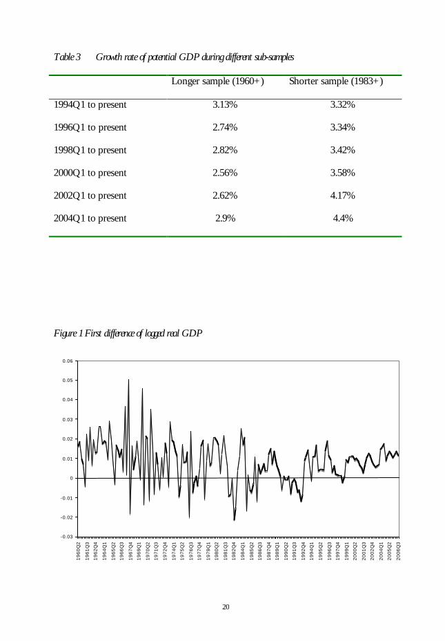
The data are seasonally adjusted quarterly time series, starting in the second quarter of

1960 and ending in the fourth quarter of 20063. Table 1 shows the variables used in the

model and Figures 1 to 3 plot the three main variables. The reduced form VAR was

estimated with four lags.

Table 1 about here

Figure 1 about here

As a further robustness check, the estimation and identification were implemented on

the entire sample starting in the second quarter of 1960 and on a sub-sample starting in

the fourth quarter of 1983. This check was carried out for two reasons. Firstly, the

important evolution of the monetary policy regime in South Africa during the early

eighties when quantitative controls were largely abandoned in favour of market-based

3 The data for the fourth quarter are an estimate.

9

instruments, as was recommended by the De Kock Commission (1985). Secondly, as

can be seen in Figure 2, there is some doubt over the covariance stationarity4 of the

fiscal policy proxy over the longer sample, a problem which is less serious in the shorter

sample (the unit root tests are reported in Appendix A).

Figure 2 about here

Figure 3 about here

As a proxy for the stance of fiscal policy we use government consumption, rather than

the deficit. Many other measures of the stance of fiscal policy, such as the budget

balance, are jointly determined with the economic cycle and are inappropriate for the

purpose at hand. Since government revenue accounts for a large portion of the joint

endogeneity between the budget balance and the economic cycle, a useful proxy of the

fiscal stance for purposes of judging the cyclicality of fiscal policy is the ratio of

government expenditure to GDP. This is also the measure used by Fatás and Mihov

(2003) to investigate the potentially destabilising role of fiscal policy in a large cross-

country study.

As a proxy for monetary policy we use the real interest rate. Alternative estimations

4 Ideally all the variables in the estimated model should be covariance stationary, which implies

that they must not have stochastic trends. Augmented Dickey-Fuller tests were used to test for

the presence of unit roots and are reported in Appendix A.

10

using the inflation rate itself were done, delivering comparable results which are

available upon request.

4. RESULTS

This section reports impulse responses and historical decompositions to support the

plausibility of the identified supply and demand shocks proposed here.

4.1 Innovation accounting

Innovation accounting entails considering the impulse responses and variance

decomposition of structural VAR models. The first task is to inspect the impulse

response functions of the identified shocks to determine whether they match

theoretical priors concerning the direction and magnitude of impact. Figure 4 below

shows the impulse responses of real GDP for each of the identified shocks and for

both the longer and shorter sample models.

Figure 4 about here

The impulse responses in Figure 4 are consistent with theoretical priors. The supply

shock has a permanent impact on real GDP, while the two components of aggregate

demand have, by construction, only transitory impacts. A positive fiscal shock has a

temporary expansionary impact on real GDP and a positive shock to the real interest

rate has a temporary contractionary impact on real output. The fiscal effect is stronger

in the longer sample, though that should be interpreted cautiously given the potential

non-stationarity of the fiscal proxy over that sample.

11

The variance decomposition of real GDP shows the proportion of the variance of real

GDP which can be accounted for by the three identified shocks over various horizons.

Table 2 contains the variance decomposition for real GDP, from which two deductions

follow. Firstly, the long-run development of real GDP is dominated by the history of

supply shocks. Secondly, over the short to medium term, fiscal shocks dominate

monetary shocks in their impact on real GDP, but only in the model estimated on the

longer sample. In the post-1983 sample the relative importance of monetary and fiscal

policy shocks are reversed.

Figure 5 about here

This difference between the variance decompositions of the shorter and longer sample

models might be due to the changing average size and variability of the three structural

shocks over the sample period. Figure 5 uses box plots by decade to show how the

distribution of these shocks has changed over time. The monetary policy shocks have

become more dispersed since the 1960s, while the opposite seems to have happened

with the GDP growth and fiscal policy shocks. A model estimated over the entire

sample period therefore combines two very different periods (with a pivotal point

around 1980) in the monetary history of South Africa. This stylised observation can be

sensibly connected with the reforms of the monetary policy regime introduced by the

De Kock commission and implemented in the course of the early to middle 1980s.

Figure 6 shows the impulse responses of the real interest rate relative to the three

identified shocks for both samples. A positive supply shock raises the real interest rate

12

temporarily in both samples. This is expected from the transitory disinflationary impact

of a positive supply shock. A positive fiscal shock lowers the real interest rate

temporarily, notably in the model estimated on the shorter sample, which suggests that

over that sample a fiscal stimulus meets with accommodating monetary policy.

Figure 6 about here

Figure 7 shows the impulse response functions for government expenditure relative to

the three identified shocks for both samples. The reaction of the fiscal proxy to a

supply shock in both samples suggests that GDP responds faster to a positive supply

shock than government expenditure. At least in the model estimated on the shorter

sample, government expenditure catches up with GDP over the medium term. The

positive response of a fiscal shock to a rise in the real interest rate might suggest a

counteracting fiscal response to a monetary policy shock, but even at its maximum, the

effect is very small and is not of great practical interest.

Figure 7 about here

4.2 Historical decomposition

The moving average representation of the structural system, i.e. equation 1, can be used

to decompose the historical real GDP series into paths attributable to each of the

identified shocks. For example, the structural VAR can be used to plot the evolution of

real GDP under the assumption that both demand shocks are zero, to yield a measure

of supply shocks to GDP which, aggregated over time and added to any non-stationary

13

drift, may construct an estimate of potential GDP. Similar historical decompositions

can be used to plot the contribution of the two demand shocks to the time path of

GDP and jointly they will yield a measure of the business cycle. Figure 8 shows the

historical decomposition of real GDP into components due to supply shocks, fiscal

shocks, and monetary shocks5.

Figure 8 about here

The major difference between the historical decompositions for the short and longer

sample models lies in the much larger contribution of fiscal shocks to GDP in the

longer sample. For example, fiscal policy has contributed positively to real GDP since

about 2000 on both estimates, but much more powerfully so in the model estimated on

the longer sample. However, in both models the supply shocks dominate fluctuations

in real GDP.

The patterns of the cumulated supply shocks are not identical in the two models but

show remarkable similarity, with both recording continued negative supply shocks from

the mid-eighties through 1994, after which positive supply shocks moved actual and

potential real GDP up. Figure 9 shows the estimated potential GDP for the shorter and

longer samples yielded by this decomposition.

5 The series for the potential output and business cycle measures are presented in Appendix B.

14

Figure 9 about here

The longer sample yields an opportunity to quantify the cumulative loss in aggregate

supply suffered by the South African economy in the twilight of apartheid. The top

graph in figure 9 shows that the generally positive supply shocks of the sixties were

reversed from 1973 onwards. Adverse international events, notably the first oil shock,

but also the collapse of the Portuguese colonies (Mozambique and Angola) which

created hostile states on the borders of South Africa, signalled the start of two decades

of adverse supply shocks. Domestic unrest in 1976 and again in the mid-1980s, the

debt standstill in 1985, and the final unravelling of the National Party’s grip on political

power were all along the path of declining potential GDP, most likely fuelled by

significant human and capital flight.

Figure 10 matches important international events, political developments, policy

decisions, and economic shocks to the cumulative supply shocks as identified by the

longer sample model. On this measurement potential GDP declined by a cumulative

30% relative to trend between the mid-seventies and the mid-nineties. In this way the

decomposition provides a unique quantification of the costs of maintaining apartheid

since the seventies, in a time of adverse international shocks. It yields a plausible

pattern and magnitude, given historical accounts of the economic costs of apartheid by

Moll (1991) and Feinstein (2005), for example.

15

Figure 10 about here

The new measure of potential GDP also shows a marked rise in potential GDP since

1994, starting almost immediately after the political transition. While the pattern differs

for the models estimated on the longer and shorter samples (the longer sample model

shows a sharper bounce in potential GDP immediately after the political transition

which flattens out after 2000, while the shorter sample model shows a slower initial

response for potential GDP but an acceleration after 2000), both imply that potential

GDP has lately been growing at a healthy rate, though well short of the goals set by the

South African government. Table 3 shows the growth rate of potential GDP for the

two models calculated over different sub-samples of the post-1994 era. The estimates in

Table 3 suggest a range of 2.5% to 4.4% for the growth rate of potential GDP, while

3.5% would be a likely point estimate (Frankel et al., 2007: 14).

Table 3 about here

In addition to examining the plausibility of the identified supply shocks, one might also

examine the plausibility of the identified demand shocks through comparison with

independent information on the South African business cycle. Following Blanchard and

Quah (1989), we compare the cumulative aggregate demand shock with the turning

points of the South African business cycle as identified by (i) the dating committee of

the SARB, and (ii) the turning points identified by Du Plessis (2006) using a non-

parametric dating algorithm applied to real GDP. Figure 11 shows the phases of the

business cycle defined with these two methods and the new measure of aggregate

16

demand is superimposed onto it

The measure of aggregate demand identified with the long-run restrictions matches the

periods of relative expansion and relative contraction in the South African economy

surprisingly well. This is particularly the case where the comparison is made with Du

Plessis’ (2006) alternative turning points, which, he has argued, capture the periods of

relative contraction and expansion in the South African GDP more accurately than the

official turning points.

The only real anomaly in the comparison is the apparent positive demand shock during

the contraction following the peak of June 1984. Du Plessis and Smit (2007) examined

the circumstances of this contraction and found that it was the only post-1980

contraction in South Africa during which the monetary authorities provided a

cumulatively large nominal and particularly real reduction in their policy interest rate.

Not all downswings are due to demand shocks (in this case the demand shock from

monetary policy was notably positive) and in this case the downswing is largely

explained by a sharp negative supply shock as identified (see Figure 10). The model as

presented here, is not sensitive enough to identify the precise nature of that supply

shock, but Frankel, Smit and Sturzenegger (2007: 11) highlight two developments that

were particularly adverse in 1984 and would have ended in the supply shock as

identified here, i.e. a precipitous decline in public investment and depressed terms of

trade.

Apart form this period, the new business cycle measure matches existing evidence

17

closely. Following Blanchard and Quah (1989: 665), we interpret this close match

between the business cycle measure, generated by the identified demand shocks, and

independent business cycle information as suggestive of the plausibility of the identified

demand shocks.

5. CONCLUSION

This paper applies a structural VAR method to identify aggregate supply and demand

shocks for the South African economy since the 1960s. The impulse responses suggest

that the identified structural shocks and system dynamics are theory consistent. Further,

the identified aggregate supply shock is used to yield a new measure of potential GDP

and of the business cycle. The new measure of potential GDP suggests that the South

African economy suffered a 30% relative decline in potential GDP between the mid-

seventies and mid-nineties as the internal and external costs of apartheid rose at a time

of disruption in the world economy. It also suggests that the present trajectory potential

GDP is growing by about 2.5% to 4.4% per year with a likely value of around 3.5%.

This order of magnitude compares favourably with some of the more recent

calculations in the literature such as Du Toit, Van Eyden and Ground (2006).

The identified demand shock was also used to create a new measure of the South

African business cycle, which matched independent information about the business

cycle. The plausible history of the new measures for the business cycle and potential

GDP support the method of identification used here.

18

Table 1 Data

Variable Calculation Source

∆yt First difference of the log

of real GDP

SARB, RB6006D

gt Ratio of government

consumption to GDP

SARB, RB6008D,

RB6006D

rt Real interest rate calculated

using monthly data and a

within-quarter formula6

SARB, Discount rate and

CPI index, RB 7032N

6 For each quarter the real interest rate was calculated using monthly data and the following formula where m t means the second month of the quarter:

Avg imt−1,imt ,imt +1( )− lnCPImt + CPImt +1

2

− ln

CPImt + CPImt−1

2

12

−1

19

Table 2 Variance decomposition of real GDP

Longer sample (1960+)

Shorter sample (1983+)

Variance Decomposition of GDPSupply Shock Fiscal Shock Monetary Shock

1 69.0% 28.3% 2.6%2 67.6% 31.4% 1.0%3 58.6% 37.0% 4.4%4 62.2% 35.2% 2.6%5 64.0% 33.3% 2.7%6 63.4% 33.6% 2.9%7 68.3% 29.9% 1.8%8 70.0% 28.1% 1.9%9 72.0% 26.5% 1.5%

10 74.7% 24.2% 1.2%11 75.9% 23.0% 1.1%12 77.6% 21.6% 0.9%13 78.9% 20.3% 0.8%14 80.1% 19.3% 0.7%15 81.3% 18.1% 0.6%20 85.9% 13.7% 0.3%30 91.6% 8.2% 0.1%50 96.6% 3.4% 0.0%75 98.7% 1.3% 0.0%100 99.5% 0.5% 0.0%

Quarter Nº

Variance Decomposition of GDPSupply Shock Fiscal Shock Monetary Shock

1 88.7% 1.0% 10.3%2 86.0% 5.1% 8.9%3 82.4% 3.0% 14.6%4 88.2% 3.7% 8.1%5 88.3% 3.3% 8.4%6 90.9% 2.4% 6.7%7 93.5% 1.5% 5.0%8 94.7% 1.2% 4.1%9 96.1% 0.6% 3.3%

10 97.3% 0.4% 2.3%11 97.8% 0.2% 2.0%12 98.4% 0.1% 1.5%13 98.8% 0.0% 1.2%14 99.0% 0.0% 1.0%15 99.2% 0.0% 0.8%20 99.7% 0.0% 0.2%30 99.9% 0.0% 0.0%50 100.0% 0.0% 0.0%75 100.0% 0.0% 0.0%

100 100.0% 0.0% 0.0%

Quarter Nº

20

Table 3 Growth rate of potential GDP during different sub-samples

Longer sample (1960+) Shorter sample (1983+)

1994Q1 to present 3.13% 3.32%

1996Q1 to present 2.74% 3.34%

1998Q1 to present 2.82% 3.42%

2000Q1 to present 2.56% 3.58%

2002Q1 to present 2.62% 4.17%

2004Q1 to present 2.9% 4.4%

Figure 1 First difference of logged real GDP

-0.03

-0.02

-0.01

0

0.01

0.02

0.03

0.04

0.05

0.06

1960Q

2

1961Q

3

1962Q

4

1964Q

1

1965Q

2

1966Q

3

1967Q

4

1969Q

1

1970Q

2

1971Q

3

1972Q

4

1974Q

1

1975Q

2

1976Q

3

1977Q

4

1979Q

1

1980Q

2

1981Q

3

1982Q

4

1984Q

1

1985Q

2

1986Q

3

1987Q

4

1989Q

1

1990Q

2

1991Q

3

1992Q

4

1994Q

1

1995Q

2

1996Q

3

1997Q

4

1999Q

1

2000Q

2

2001Q

3

2002Q

4

2004Q

1

2005Q

2

2006Q

3

21

Figure 2 Ratio of government expenditure to GDP

0.1

0.12

0.14

0.16

0.18

0.2

0.22

0.24

1960Q

2

1961Q

3

1962Q

4

1964Q

1

1965Q

2

1966Q

3

1967Q

4

1969Q

1

1970Q

2

1971Q

3

1972Q

4

1974Q

1

1975Q

2

1976Q

3

1977Q

4

1979Q

1

1980Q

2

1981Q

3

1982Q

4

1984Q

1

1985Q

2

1986Q

3

1987Q

4

1989Q

1

1990Q

2

1991Q

3

1992Q

4

1994Q

1

1995Q

2

1996Q

3

1997Q

4

1999Q

1

2000Q

2

2001Q

3

2002Q

4

2004Q

1

2005Q

2

2006Q

3

22

Figure 3 Real interest rate

-20

-15

-10

-5

0

5

10

15

20

1960

/02

1961

/05

1962

/08

1963

/11

1965

/02

1966

/05

1967

/08

1968

/11

1970

/02

1971

/05

1972

/08

1973

/11

1975

/02

1976

/05

1977

/08

1978

/11

1980

/02

1981

/05

1982

/08

1983

/11

1985

/02

1986

/05

1987

/08

1988

/11

1990

/02

1991

/05

1992

/08

1993

/11

1995

/02

1996

/05

1997

/08

1998

/11

2000

/02

2001

/05

2002

/08

2003

/11

2005

/02

2006

/05

23

Figure 4 Impulse response of real GDP for each of the identified shocks

Longer sample (1960+) Shorter sample (1983+)

1 9 17 25 33 41 49 57 65 73 81 89 97

Accumulated Response of GDP to Supply Shock

1 9 17 25 33 41 49 57 65 73 81 89 97

Accumulated Response of GDP to Supply Shock

1 9 17 25 33 41 49 57 65 73 81 89 97

Accumulated Response of GDP to Fiscal Shock

1 9 17 25 33 41 49 57 65 73 81 89 97

Accumulated Response of GDP to F iscal Shock

1 9 17 25 33 41 49 57 65 73 81 89 97

Accumulated Response of GDP to Monetary Shock

1 9 17 25 33 41 49 57 65 73 81 89 97

Accumulated Response of GDP to Monetary Shock

24

Figure 5 Box plot of structural shocks to the three variables by decade

25

Figure 6 Impulse response of the real interest rate for each of the identified shocks

Longer sample (1960+) Shorter sample (1983+)

1 9 17 25 33 41 49 57 65 73 81 89 97

Response of Real Interest Rate to Supply Shock

1 9 17 25 33 41 49 57 65 73 81 89 97

Response of Real Interest Rate to Supply Shock

1 9 17 25 33 41 49 57 65 73 81 89 97

Response of Real Interest Rate to Fiscal Shock

1 9 17 25 33 41 49 57 65 73 81 89 97

Response of Real Interest Rate to Fiscal Shock

1 9 17 25 33 41 49 57 65 73 81 89 97

Response of Real Interest Rate to Monetary Shock

1 9 17 25 33 41 49 57 65 73 81 89 97

Response of Real Interest Rate to Monetary Shock

26

Figure 7 Impulse response of government consumption to real GDP for each of the identified shocks

Longer sample (1960+) Shorter sample (1983+)

1 9 17 25 33 41 49 57 65 73 81 89 97

Response of Gov. Cons. as percentage of GDP to Supply Shock

1 9 17 25 33 41 49 57 65 73 81 89 97

Response of Gov. Cons. as percentage of GDP to Supply Shock

1 9 17 25 33 41 49 57 65 73 81 89 97

Response of Gov. Cons. as percentage of GDP to Fiscal Shock

1 9 17 25 33 41 49 57 65 73 81 89 97

Response of Gov. Cons. as percentage of GDP to Fiscal Shock

1 9 17 25 33 41 49 57 65 73 81 89 97

Response of Gov. Cons. as percentage of GDP to Monetary Shock

1 9 17 25 33 41 49 57 65 73 81 89 97

Response of Gov. Cons. as percentage of GDP to Monetary Shock

27

Figure 8 Historical decomposition of real GDP

Longer sample (1960+)

Shorter sample (1983+)

1961

:02

1963

:02

1965

:02

1967

:02

1969

:02

1971

:02

1973

:02

1975

:02

1977

:02

1979

:02

1981

:02

1983

:02

1985

:02

1987

:02

1989

:02

1991

:02

1993

:02

1995

:02

1997

:02

1999

:02

2001

:02

2003

:02

2005

:02

Supply Shock Fiscal Shock Monetary Shock

1961

:02

1963

:02

1965

:02

1967

:02

1969

:02

1971

:02

1973

:02

1975

:02

1977

:02

1979

:02

1981

:02

1983

:02

1985

:02

1987

:02

1989

:02

1991

:02

1993

:02

1995

:02

1997

:02

1999

:02

2001

:02

2003

:02

2005

:02

Supply Shock Fiscal Shock Monetary Shock

28

Figure 9 New measure of aggregate supply

Longer sample (1960+)

Shorter sample (1983+)

13

200013

400013

600013

800013

1000013

1200013

140001319

61:2

1963

:2

1965

:2

1967

:2

1969

:2

1971

:2

1973

:2

1975

:2

1977

:2

1979

:2

1981

:2

1983

:2

1985

:2

1987

:2

1989

:2

1991

:2

1993

:2

1995

:2

1997

:2

1999

:2

2001

:2

2003

:2

2005

:2

Mil

lio

ns

of

Ran

d (

Co

nn

stan

t 20

00 p

rice

s)

Acc. Response of GDP to Supply Shock + Forecast

600000

700000

800000

900000

1000000

1100000

1200000

1300000

1984

:4

1986

:4

1988

:4

1990

:4

1992

:4

1994

:4

1996

:4

1998

:4

2000

:4

2002

:4

2004

:4

2006

:4

Mill

ion

s o

f R

and

(C

on

stan

t 20

00 p

rice

s)

Acc. Response of GDP to Supply Shock + Forecast

\

29

Figure 10 Events associated with supply shocks to the South African economy

30

Figure 11 New measure of aggregate demand

Longer sample (1960+) Shorter sample (1983+)

Longer sample (1960+) Shorter sample (1983+)

-0.08

-0.06

-0.04

-0.02

0

0.02

0.04

0.06

19

61

:2

19

63

:21

96

5:2

19

67

:2

19

69

:2

19

71

:21

97

3:2

19

75

:2

19

77

:21

97

9:2

19

81

:2

19

83

:2

19

85

:21

98

7:2

19

89

:2

19

91

:21

99

3:2

19

95

:2

19

97

:21

99

9:2

20

01

:2

20

03

:2

20

05

:2

0.00%

0.20%

0.40%

0.60%

0.80%

1.00%

Expansions (SARB) Accumulated Response of GDP to Fiscal & Monetary Shocks

-0.08

-0.06

-0.04

-0.02

0

0.02

0.04

0.06

1961

:219

63:2

1965

:219

67:2

1969

:2

1971

:219

73:2

1975

:219

77:2

1979

:219

81:2

1983

:219

85:2

1987

:219

89:2

1991

:219

93:2

1995

:219

97:2

1999

:220

01:2

2003

:220

05:2

0.00%

0.20%

0.40%

0.60%

0.80%

1.00%

Expansions (Alternative) Accumulated Response of GDP to Fiscal & Monetary Shocks

-0.030

-0.025

-0.020

-0.015

-0.010-0.005

0.0000.005

0.0100.015

0.020

0.025

19

84

:4

19

86

:4

19

88

:4

19

90

:4

19

92

:4

19

94

:4

19

96

:4

19

98

:4

20

00

:4

20

02

:4

20

04

:4

20

06

:4

00.10.20.30.40.50.60.70.80.91

Expansions (SARB)

A ccumulated Response of GDP to Fis cal & Monetary Shocks

-0.030

-0.025

-0.020

-0.015

-0.010

-0.005

0.000

0.005

0.010

0.015

0.020

0.025

19

84

:4

19

86

:4

19

88

:4

19

90

:4

19

92

:4

19

94

:4

19

96

:4

19

98

:4

20

00

:4

20

02

:4

20

04

:4

00.10.20.30.40.50.60.70.80.91

Expansions (Alternat ive)

Ac cumulated Response of GDP to Fisc al & Monetary Shocks

31

APPENDIX A

Augmented Dickey-Fuller tests were used to test the null hypothesis of a unit root in

the series used here, the results of which are reported in Table 2. There is no evidence

of unit roots either in the real GDP differenced series or in the series for real interest

rates, but it is not possible to reject the hypothesis of a unit root for the fiscal policy

proxy. This raises a concern over the stability of the VAR. Of course, there may be

concern over the low power of unit root tests, and thus for a variable such as

government expenditure over GDP, it is unlikely to drift forever away from a

reasonably stable value. However, to determine how serious this may be, we computed

the eigenvalues of the SVAR system. We found that all the eigenvalues lie within the

unit circle, and therefore there does not seem to be a risk of VAR instability, despite the

unit root test results.

Table 2 Unit root tests

ADF critical values Variable Sample

No. deterministic

components

Constant Constant and

trend

∆yt 1960+ -2.691*** -4.656** -5.007***

∆yt 1984+ -2.155** -3.499** -4.339***

gt 1960+ 1.319 -1.605 -1.251

gt 1984+ 0.101 -1.856 -2.082

rt 1960+ -3.348*** -3.874*** -4.438***

rt 1984+ -2.453** -3.336** -4.313***

The Augmented Dickey-Fuller statistics were estimated with four lags.

*** Significant at the 1% level, ** Significant at the 5% level, * Significant at the 10% level

32

APPENDIX B

The following table shows the historical decomposition of the South African real GDP

for both versions of the SVAR estimated here. Table B.1 shows real GDP, the implied

measure of potential GDP and the implied business cycle measure for the model

estimated over the longer sample, while table B.2 shows the same for the model

estimated over the shorter sample.

Table B.1 Historical decomposition of real GDP, 1960+ model Date Real

GDP Potential GDP

Output Gap

Date Real GDP Potential GDP

Output Gap

1961Q1 280645 1984Q1 712,246 707,749 4,497 1961Q2 279418 283167 -3749 1984Q2 727,042 714,400 12,642 1961Q3 285659 283449 2210 1984Q3 714,992 728,019 -13,027 1961Q4 288256 290732 -2476 1984Q4 716,097 714,684 1,413 1962Q1 295712 292920 2792 1985Q1 711,831 714,610 -2,779 1962Q2 297606 299595 -1989 1985Q2 706,655 708,350 -1,695 1962Q3 303416 302913 503 1985Q3 704,790 706,933 -2,143 1962Q4 307302 306557 745 1985Q4 712,326 705,216 7,110 1963Q1 311367 311769 -402 1986Q1 703,840 708,664 -4,824 1963Q2 319600 317527 2073 1986Q2 708,699 706,771 1,928 1963Q3 328035 325041 2994 1986Q3 710,294 706,866 3,428 1963Q4 333815 334466 -651 1986Q4 713,276 712,693 583 1964Q1 340068 337771 2297 1987Q1 718,464 715,712 2,752 1964Q2 346223 345497 726 1987Q2 721,026 718,399 2,627 1964Q3 349476 350386 -910 1987Q3 723,657 725,103 -1,446 1964Q4 359695 355056 4639 1987Q4 732,541 728,796 3,745 1965Q1 366616 367366 -750 1988Q1 743,550 739,377 4,173 1965Q2 370162 370889 -727 1988Q2 748,830 749,396 -566 1965Q3 368994 374783 -5789 1988Q3 758,901 752,597 6,304 1965Q4 375131 373424 1707 1988Q4 766,027 763,268 2,759 1966Q1 380399 380678 -279 1989Q1 770,771 766,328 4,443 1966Q2 384539 385573 -1034 1989Q2 774,115 772,109 2,006 1966Q3 390204 389833 371 1989Q3 774,737 779,949 -5,212 1966Q4 391488 396036 -4548 1989Q4 769,943 775,540 -5,597 1967Q1 405721 399068 6653 1990Q1 770,559 769,851 708 1967Q2 406366 411623 -5257 1990Q2 769,923 777,447 -7,524 1967Q3 426799 414815 11984 1990Q3 769,276 770,191 -915 1967Q4 419050 433949 -14899 1990Q4 769,990 768,754 1,236 1968Q1 425930 424204 1726 1991Q1 763,866 771,276 -7,410 1968Q2 427818 432497 -4679 1991Q2 762,142 762,986 -844 1968Q3 432436 433126 -690 1991Q3 761,846 762,718 -872 1968Q4 440612 438117 2495 1991Q4 760,536 757,442 3,094 1969Q1 443778 445886 -2108 1992Q1 755,206 763,368 -8,162 1969Q2 443404 448967 -5563 1992Q2 750,574 755,680 -5,106 1969Q3 463653 453410 10243 1992Q3 741,884 751,311 -9,427 1969Q4 457395 466872 -9477 1992Q4 735,580 745,938 -10,358 1970Q1 467240 463084 4156 1993Q1 742,097 736,393 5,704 1970Q2 476774 474001 2773 1993Q2 750,237 741,863 8,374 1970Q3 471270 480793 -9523 1993Q3 761,036 757,883 3,153

33

1970Q4 487852 478221 9631 1993Q4 766,675 764,697 1,978 1971Q1 495078 495523 -445 1994Q1 765,582 768,591 -3,009 1971Q2 491042 495761 -4719 1994Q2 773,888 770,962 2,926 1971Q3 497438 495875 1563 1994Q3 782,592 772,707 9,885 1971Q4 501,014 502,783 -1,769 1994Q4 795,654 791,452 4,202 1972Q1 498,060 507,077 -9,017 1995Q1 798,528 801,723 -3,195 1972Q2 503,271 502,753 518 1995Q2 802,074 807,016 -4,942 1972Q3 503,582 505,273 -1,691 1995Q3 805,536 815,626 -10,090 1972Q4 512,500 509,763 2,737 1995Q4 808,715 810,934 -2,219 1973Q1 519,110 515,558 3,552 1996Q1 820,063 816,103 3,960 1973Q2 516,801 524,457 -7,656 1996Q2 835,424 827,319 8,105 1973Q3 531,747 523,353 8,394 1996Q3 844,904 841,808 3,096 1973Q4 541,990 536,596 5,394 1996Q4 852,917 848,159 4,758 1974Q1 552,117 546,061 6,056 1997Q1 855,368 859,269 -3,901 1974Q2 559,706 557,263 2,443 1997Q2 860,600 864,740 -4,140 1974Q3 566,045 561,454 4,591 1997Q3 862,397 869,707 -7,310 1974Q4 560,702 569,544 -8,842 1997Q4 863,699 871,166 -7,467 1975Q1 558,456 565,891 -7,435 1998Q1 864,791 871,465 -6,674 1975Q2 568,083 560,360 7,723 1998Q2 866,014 872,349 -6,335 1975Q3 572,631 572,873 -242 1998Q3 864,116 859,779 4,337 1975Q4 577,353 576,964 389 1998Q4 864,951 873,521 -8,570 1976Q1 584,941 580,970 3,971 1999Q1 872,905 879,230 -6,325 1976Q2 573,271 585,180 -11,909 1999Q2 879,852 883,014 -3,162 1976Q3 586,910 578,782 8,128 1999Q3 889,461 894,597 -5,136 1976Q4 582,621 592,304 -9,683 1999Q4 899,242 895,557 3,685 1977Q1 581,348 584,227 -2,879 2000Q1 909,357 906,289 3,068 1977Q2 581,907 584,011 -2,104 2000Q2 917,724 913,835 3,889 1977Q3 579,661 585,840 -6,179 2000Q3 926,813 924,461 2,352 1977Q4 582,638 578,689 3,949 2000Q4 934,698 935,643 -945 1978Q1 592,219 591,355 864 2001Q1 940,768 942,358 -1,590 1978Q2 603,664 598,298 5,366 2001Q2 945,471 949,205 -3,734 1978Q3 597,170 599,191 -2,021 2001Q3 947,982 958,571 -10,589 1978Q4 602,605 602,585 20 2001Q4 955,271 953,068 2,203 1979Q1 613,153 607,610 5,543 2002Q1 965,346 956,339 9,007 1979Q2 617,114 618,077 -963 2002Q2 977,594 968,088 9,506 1979Q3 621,720 615,392 6,328 2002Q3 988,659 981,114 7,545 1979Q4 634,479 625,926 8,553 2002Q4 996,885 993,695 3,190 1980Q1 647,514 644,735 2,779 2003Q1 1,003,734 1,009,525 -5,791 1980Q2 659,823 649,345 10,478 2003Q2 1,009,319 1,019,042 -9,723 1980Q3 671,120 665,270 5,850 2003Q3 1,015,432 1,021,499 -6,067 1980Q4 672,628 669,836 2,792 2003Q4 1,022,567 1,028,894 -6,327 1981Q1 680,982 684,229 -3,247 2004Q1 1,037,622 1,029,023 8,599 1981Q2 695,854 689,418 6,436 2004Q2 1,054,288 1,046,140 8,148 1981Q3 705,981 696,186 9,795 2004Q3 1,072,821 1,068,462 4,359 1981Q4 710,386 714,617 -4,231 2004Q4 1,082,341 1,077,836 4,505 1982Q1 703,805 712,172 -8,367 2005Q1 1,094,907 1,093,412 1,495 1982Q2 697,932 706,267 -8,335 2005Q2 1,109,662 1,107,209 2,453 1982Q3 697,754 704,000 -6,246 2005Q3 1,123,529 1,115,994 7,535 1982Q4 683,003 697,937 -14,934 2005Q4 1,135,402 1,134,710 692 1983Q1 672,461 684,804 -12,343 2006Q1 1,149,336 1,148,473 863 1983Q2 675,253 676,992 -1,739 2006Q2 1,164,856 1,153,124 11,732 1983Q3 683,038 679,034 4,004 2006Q3 1,178,196 1,172,574 5,622 1983Q4 700,362 689,333 11,029

34

Table B.2 Historical decomposition of real GDP, 1983+ model Date Real

GDP Potential GDP

Output Gap

Date Real GDP Potential GDP

Output Gap

1984Q3 714,992 1995Q4 808,715 812,648 -3,933 1984Q4 716,097 715,862 235 1996Q1 820,063 819,265 798 1985Q1 711,831 711,712 119 1996Q2 835,424 831,189 4,235 1985Q2 706,655 707,126 -471 1996Q3 844,904 844,840 64 1985Q3 704,790 703,934 856 1996Q4 852,917 852,027 890 1985Q4 712,326 712,971 -645 1997Q1 855,368 857,167 -1,799 1986Q1 703,840 707,721 -3,881 1997Q2 860,600 862,011 -1,411 1986Q2 708,699 706,500 2,199 1997Q3 862,397 867,317 -4,920 1986Q3 710,294 712,618 -2,324 1997Q4 863,699 869,058 -5,359 1986Q4 713,276 715,099 -1,823 1998Q1 864,791 868,182 -3,391 1987Q1 718,464 716,748 1,716 1998Q2 866,014 869,456 -3,442 1987Q2 721,026 722,329 -1,303 1998Q3 864,116 864,621 -505 1987Q3 723,657 727,253 -3,596 1998Q4 864,951 867,599 -2,648 1987Q4 732,541 733,319 -778 1999Q1 872,905 871,124 1,781 1988Q1 743,550 741,232 2,318 1999Q2 879,852 881,271 -1,419 1988Q2 748,830 749,096 -266 1999Q3 889,461 887,406 2,055 1988Q3 758,901 758,177 724 1999Q4 899,242 895,363 3,879 1988Q4 766,027 762,934 3,093 2000Q1 909,357 902,938 6,419 1989Q1 770,771 768,964 1,807 2000Q2 917,724 913,121 4,603 1989Q2 774,115 772,880 1,235 2000Q3 926,813 924,856 1,957 1989Q3 774,737 772,693 2,044 2000Q4 934,698 932,912 1,786 1989Q4 769,943 769,680 263 2001Q1 940,768 940,219 549 1990Q1 770,559 766,905 3,654 2001Q2 945,471 943,960 1,511 1990Q2 769,923 770,718 -795 2001Q3 947,982 949,437 -1,455 1990Q3 769,276 771,874 -2,598 2001Q4 955,271 953,100 2,171 1990Q4 769,990 768,419 1,571 2002Q1 965,346 964,053 1,293 1991Q1 763,866 762,680 1,186 2002Q2 977,594 976,058 1,536 1991Q2 762,142 758,672 3,470 2002Q3 988,659 990,264 -1,605 1991Q3 761,846 760,235 1,611 2002Q4 996,885 1,000,712 -3,827 1991Q4 760,536 759,002 1,534 2003Q1 1,003,734 1,006,929 -3,195 1992Q1 755,206 758,851 -3,645 2003Q2 1,009,319 1,015,263 -5,944 1992Q2 750,574 752,041 -1,467 2003Q3 1,015,432 1,018,659 -3,227 1992Q3 741,884 745,823 -3,939 2003Q4 1,022,567 1,022,961 -394 1992Q4 735,580 737,725 -2,145 2004Q1 1,037,622 1,033,262 4,360 1993Q1 742,097 738,799 3,298 2004Q2 1,054,288 1,049,575 4,713 1993Q2 750,237 743,953 6,284 2004Q3 1,072,821 1,069,526 3,295 1993Q3 761,036 758,532 2,504 2004Q4 1,082,341 1,080,983 1,358 1993Q4 766,675 766,010 665 2005Q1 1,094,907 1,093,305 1,602 1994Q1 765,582 767,155 -1,573 2005Q2 1,109,662 1,107,435 2,227 1994Q2 773,888 773,555 333 2005Q3 1,123,529 1,120,809 2,720 1994Q3 782,592 781,234 1,358 2005Q4 1,135,402 1,133,819 1,583 1994Q4 795,654 795,213 441 2006Q1 1,149,336 1,150,461 -1,125 1995Q1 798,528 801,598 -3,070 2006Q2 1,164,856 1,162,177 2,679 1995Q2 802,074 807,906 -5,832 2006Q3 1,178,196 1,176,693 1,503 1995Q3 805,536 810,112 -4,576

35

REFERENCES

Akinboade, O. A. (2005). "Some estimates of potential output and the output gap for South Africa." Journal for Studies in Economics and Econometrics, 29(1): 15-28. Arora, V. and A. Bhundia (2003). Potential Output and Total Factor Productivity Growth in Post-Apartheid South Africa. Washington, IMF working paper: WP/03/178. Blanchard, O. J. and D. Quah (1989). "The Dynamic Effects of Aggregate Demand and Supply Disturbances." American Economic Review, 79(4): 655-673. Burger, P. and M. Marinkov (2006). "The South African Phillips curve: how applicable is the Gordon model?" South African Journal of Economics, 74(2): 172-189. Clarida, R. and J. Galí (1994). "Sources of Real Exchange Rate Fluctuations: How Important are nominal Shocks?" Carnegie-Rochester Conference Series on Public Policy, 41: 1-56. De Jager, B. and D. Smal (1984). "Potential Gross Domestic Product of South Africa." South African Reserve Bank Quarterly Bulletin, 154: 59-79. De Kock Commission (1985). Final report of the commission of inquiry into the monetary system and monetary policy in South Africa (RP 70/1984). Pretoria, Government Printer. Du Plessis, S. A. (2006). "Reconsidering the business cycle and stabilisation policies in South Africa." Economic Modelling, 23(5): 761-774. Du Plessis, S. A. and B. W. Smit (2007). "Countercyclical Monetary Policy in South Africa." Journal for Studies in Economics and Econometrics, 31(1): 79-98. Du Toit, C. B. and E. Moolman (2003). "Estimating potential output and capacity utilization for the South African economy." South African Journal of Economics, 71(1): 96-118. Du Toit, C. B., R. Van Eyden and M. Ground (2006). Does South Africa have the potential and capacity to grow at 7 per cent: A labour market perspective. Pretoria, Department of Economics Working Paper Series No 2006-03, University of Pretoria. DuPasquier, C., A. Guay and P. St-Amant (1999). "A Survey of Alternative Methodologies for Estimating Potential Output and the Output Gap." Journal of Macroeconomics, 21(3): 577-595. Fatás, A. and I. Mihov (2003). "The case for restricting fiscal policy discretion." Quarterly Journal of Economics, 2003(November): 1419-1447.

36

Fedderke, J. W. and E. Schaling (2005). "Modelling inflation in South Africa: a multivariate cointegation analysis." South African Journal of Economics, 73(1): 79-92. Feinstein, C. H. (2005). An economic history of South Africa: Conquest, discrimination and development. Cambridge, Cambridge University Press. Frankel, J., B. W. Smit and F. Sturzenegger (2007). South Africa: Macroeconomic Challenges after a Decade of Success. Cambridge MA, CID Working Paper No. 133, April 2007. Galí, J. (1992). "How Well Does the IS-LM Model Fit U.S. Data?" Quarterly Journal of Economics, 107(May): 709-738. Geldenhuys, J. P. and M. Marinkov (2006). Robust estimates of Oken’s Coefficient for South Africa, DPRU Conference Paper, October 2006. Kaseeram, I., T. Nichola and S. Mainardi (2004). "South African inflationary dynamics and the pass-through effects from depreciation to unit labour costs." South African Journal of Economics, 72(1): 85-107. King, R. G., C. I. Plosser, J. H. Stock and M. W. Watson (1991). "Stochastic Trends and Economic Fluctuations." American Economic Review, 81(4): 819-840. Knedlik, T. (2006). "Estimating monetary policy rules for South Africa." South African Journal of Economics, 74(4): 629-641. Moll, T. (1991). "Did the apartheid economy 'fail'?" Journal of Southern African Studies, 17(2): 271-291. Shapiro, M. D. and M. W. Watson (1988). Sources of Business Cycles Fluctuations. In: S. Fischer (eds.). NBER Macroeconomics Annual, The MIT Press. 1988. Smit, B. W. and L. Burrows (2002). Estimating potential output and output gaps for the South African economy. Stellenbosch, Stellenbosch Economic Working Paper, No 5/2002, Stellenbosch University. Woglom, G. (2005). "Forecasting South African inflation." South African Journal of Economics, 73(2): 302-320.