Identifying Aggregate Liquidity Shocks with Monetary ... · Identifying Aggregate Liquidity Shocks...

- Logo - CMYK.png - Logo - CMYK.png

Introduction Data Model & Identification Results Robustness Conclusions

Identifying Aggregate Liquidity Shocks withMonetary Policy Shocks: An Application using UK

Data

Michael Ellington and Costas Milas

Financial Services, Liquidity and Economic ActivityBank of England

May 24, 2017



Motivation & Related Literature

How to capture unconventional monetary policies in a VARmodel using data before 2009?

Liquidity

Kiyotaki and Moore (2012); Shi (2015); Baumeister et al.(2008); Adalid and Detken (2007)

Monetary Policy and Sign Restrictions

Canova and De Nicolo (2002); Uhlig (2005)

Uconventional Monetary Policies

Gambacorta et al. (2014); Weale and Wieladek (2016)



Contribution & Key Findings

We propose an aggregate liquidity shock in conjunction witha traditional monetary policy shock in a structural VARmodel.Findings:

Substantial evidence in favour of a time-varying transmission ofaggregate liquidity shocks

Statistically significant differences in the contribution of aggregateliquidity shocks to macroeconomic variation at a business cyclefrequency

Aggregate liquidity shocks contribute 32% and 47% to the varianceof GDP and inflation at business cycle frequencies following the2008 recession, respectively

During the Great Recession, the economic significance of theseshocks for GDP and inflation forecast error variances are 14 and 13times greater relative to shocks identified using a Choleskydecomposition



Data

Our estimated model uses UK data from 1976Q1-2016Q4 on:quarterly real GDP growth, yt ; consumer price inflation, πt ; ourconstruction of a break adjusted M4/M4ex (which excludes otherintermediate financial corporations) series, mt ; and the Bank ofEngland Bank rate, it .

1976 1996 2016

−2

0

2

4

Perc

ent

yt

1976 1996 20160

2

4

6

8πt

1976 1996 2016−2

0

2

4

6

Time

Perc

ent

mt

1976 1996 20160

2

4

Time

it



The Model I

We work with the following TVP–VAR model with 2 lags and 4variables:

Yt = β0,t + β1,tYt−1 + β2,tYt−2 + εt ≡ X′t θt + εt

the VAR’s time–varying parameters are collected in θt and evolveas

p(θt |θt−1,Q) = I (θt)f (θt |θt−1,Q)

θt = θt−1 + νt

The innovations εt v N(0,Ωt). Ωt is the time–varying covariancematrix which we factor as

Var(εt) ≡ Ωt = A−1t Ht(A

−1t )

′



The Model II

Collecting the non-unit and non-zero elements in At in the vectorαt = [α2,1,t , ..., α4,3,t ]

′ and the diagonal elements of Ht inht = [h1,t , ..., h4,t ]

′, they evolve as

αt = αt−1 + ζt

ln ht = ln ht−1 + ηt

The innovations in the model are jointly Normalutνtζtηt

v N(0,V ), V =

IM 0 0 00 Q 0 00 0 S 00 0 0 W

where ut is such that, εt ≡ A−1

t H12t ut ; Q, S , W are positive

definite matrices.



Our Proposed Identification Scheme I

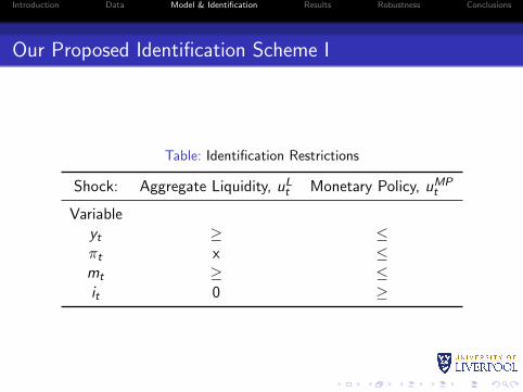
Table: Identification Restrictions

Shock: Aggregate Liquidity, uLt Monetary Policy, uMPt

Variableyt ≥ ≤πt x ≤mt ≥ ≤it 0 ≥



Our Proposed Identification Scheme II

Let

Ωt = PtDtP′t

be eigenvalue-eigenvector decomposition of Ωt .Draw an M ×M matrix K from the N(0, 1) distribution andcompute the QR decomposition of K . The time-varying structuralimpact matrix is

A0,t = PtD12t Q′



Our Proposed Identification Scheme III

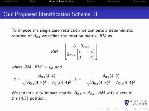
To impose the single zero restriction we compute a deterministicrotation of A0,t we define the rotation matrix, RM as

RM =

I2 02×2

02×2

[c − ss c

]where RM · RM ′ = IM and

c =A0,t(4, 4)√

A0,t(4, 3)2 + A0,t(4, 4)2, s = − A0,t(4, 3)√

A0,t(4, 3)2 + A0,t(4, 4)2

We obtain a new impact matrix, A0,t = A0,t · RM with a zero inthe (4,3) position.



Prior Information

To calibrate the model, we use the OLS estimates from aconstant parameter VAR using the first 20 years of data from1955Q4-1975Q4

Our prior specifications are similar to that of Baumeister andPeersman (2013)

We allow for 100,000 runs of the Markov Chain Monte CarloSimulation burning the first 50,000

Of the remaining 50,000 we sample every 10th draw to reduceautocorrelation



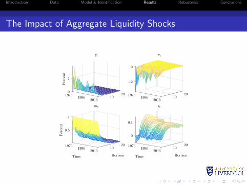
The Impact of Aggregate Liquidity Shocks

1976 1996 201610

200

1

Perc

ent

yt

1976 1996 201610

20

−2

0

πt

1976 1996 201610

20

0.5

1

Time Horizon

Perc

ent

mt

1976 1996 201610

20

0

0.1

Time Horizon

it



Historical Decomposition of Aggregate Liquidity Shocks

To interpret the figure on the next slide:

The dashed line reports the actual time series relative to itsfitted value

The solid line shows the cumulative effects of aggregateliquidity shocks on the evolution of each variable, whileturning off all other shocks

Therefore, the figure shows how the variable in question wouldhave evolved if only aggregate liquidity shocks occurred(therefore aggregate liquidity shocks have zero contributiontoward movements in the interest rate)

The difference between the dashed and solid line represents thecontribution all other shocks.



Historical Contribution of Aggregate Liquidity Shocks

1976 1996 2016−4

−2

0

2

4Pe

rcen

t

Real GDP growth

1976 1996 2016−2

0

2

4CPI Inflation

1976 1996 2016−2

−1

0

1

2

Time

Perc

ent

M4/M4ex growth

1976 1996 2016−0.4

−0.2

0

0.2

0.4

Time

Interest Rate

Contribution of aggregate liquidity shocksActual demeaned data



Does our Identified Shock Capture Quantitative Easing?

Had policymakers chosen not to implement successive roundsof Quantitative Easing, the volatility of aggregate liquidityshocks would have been less turbulent

Therefore to determine whether our proposed shock capturesunconventional monetary policies we report results from acounterfactual simulation changing the volatility of theseshocks following the Great Recession

We set the standard deviation of structural liquidity shocksfrom 2009Q1-2016Q4 to the average volatility of these shocksfrom 1976Q1-2008Q4



Does our Identified Shock Capture Quantitative Easing?

The blue line represents the median counterfactual path hadno asset purchase facilities been implemented

The red line is the simulated actual history implied by ourmodel

2009 2016−2

−1.5

−1

−0.5

0

0.5

1

1.5

Perc

ent

yt

2009 2016−1

−0.5

0

0.5

1

1.5

2

2.5πt

2009 2016−2

−1

0

1

2

3mt

median counterfactual pathsimulated actual history



Business Cycle Frequency Variance Decomposition

Following Hamilton (1994) we define business cycle frequency as10 quarters

1976 1996 20160

20

40

Perc

ent

yt

1976 1996 20160

20

40

60

πt

1976 1996 20160

20

40

Time

Perc

ent

mt

1976 1996 20160

5

10

15

Time

it

Posterior median contribution at business cycle frequency



Robustness

Our robustness analysis reveals:

Aggregate liquidity shocks retrieved from a Choleskydecomposition are not well defined and yield little economicsignificance

Our contemporaneous zero restriction on the interest rate isplausible (from historical decompositions using a Choleskydecomposition thereby allowing for liquidity shocks to affect iton impact)

There are no statistically significant differences in our resultswhen replacing M4/M4ex with Divisia money



Conclusions

Real GDP and inflation become more sensitive to aggregateliquidity shocks during recessions

These shocks hold historical importance by contributingsignificantly to macroeconomic movements, and variance

Counterfactual simulations indicate our shocks captureunconventional monetary policies, our estimates imply therecovery in GDP growth following QE1 would have been moregradual

At the onset of the Great Recession, aggregate liquidityshocks explain 32% and 47% of the variance in GDP andinflation at business cycle frequencies respectively



Extensions of our Work on Liquidity Shocks

In a ‘sister’ paper On Stock Market Illiquidity Shocks and UKMacroeconomic Dynamics, we examine the impact of illiquidityshocks in a time-varying parameter VAR model accounting for thefinancial sector by including proxies for stock market liquidity. Ourresults show:

Illiquidity shocks cause real GDP growth and inflation tocontract by 2% and 2.6% in 2008Q4

From 2010Q4–2016Q4, the percent of forecast error varianceexplained by these shocks for GDP growth and inflationvariability are 22% and 27%, respectively

There are statistically significant differences in FEVDsindicating that the importance of illiquidity shocks move withthe business cycle



Monetary Policy Shocks under our Identification Scheme

1976 1996 201610

20

−1

0Pe

rcen

tyt

1976 1996 201610

20

−2

−1

0

πt

1976 1996 201610

20

−2

−1

0

Time Horizon

Perc

ent

mt

1976 1996 201610

20−0.2

0

0.2

Time Horizon

it

Identifying Aggregate Liquidity Shocks with Monetary ... · Identifying Aggregate Liquidity Shocks...

Documents

Transcript of Identifying Aggregate Liquidity Shocks with Monetary ... · Identifying Aggregate Liquidity Shocks...