Wayne State University

Wayne State University Dissertations

1-1-2011

Identification, state estimation, and adaptive controlof type i diabetic patientsAli Mohamad HaririWayne State University,

Follow this and additional works at: http://digitalcommons.wayne.edu/oa_dissertations

Part of the Electrical and Computer Engineering Commons

This Open Access Dissertation is brought to you for free and open access by DigitalCommons@WayneState. It has been accepted for inclusion inWayne State University Dissertations by an authorized administrator of DigitalCommons@WayneState.

Recommended CitationHariri, Ali Mohamad, "Identification, state estimation, and adaptive control of type i diabetic patients" (2011). Wayne State UniversityDissertations. Paper 412.

IDENTIFICATION, STATE ESTIMATION, AND ADAPTIVE CONTROL OF TYPE ‘I’

DIABETIC PATIENTS

by

ALI MOHAMAD HARIRI

DISSERTATION

Submitted to the Graduate School

of Wayne State University,

Detroit, Michigan

in partial fulfillment of the requirements

for the degree of

DOCTOR OF PHILOSOPHY

2012

MAJOR: ELECTRICAL ENGINEERING

Approved by:

Advisor Date

© COPYRIGHT BY

ALI MOHAMAD HARIRI

2012

All Rights Reserved

ii

DEDICATION

To my parents

my wife

and my family

iii

ACKNOWLEDGEMENTS

There are several people who deserve my heartfelt thanks for their generous contributions

and support to this dissertation. First of all, I would like to express my sincere appreciation to my

respectful advisor, Professor Le Yi Wang, for his directions, suggestions, corrections,

supervision and support from the preliminary to the concluding level that enabled me to develop

an understanding of the subject. Without his guidance, I do not believe this thesis would have

been completed. Professor Wang‟s dedication and flexibility is what made it possible for me to

succeed. He was always there when I needed his advice, even after hours and outside university.

Also, I would like to thank my dissertation committee: Professor Ece Yaprak, Professor Harpreet

Singh and Professor Pepe Siy for their helpful comments and encouragement. I must express my

gratitude and deep appreciation to Dr. Eid Al-Radadi whose friendship, hospitality, knowledge

have supported, enlightened, and entertained me over the many years of our friendship.

Many thanks go to my father and my brothers and sisters for their moral support and

encouragement. My lovely daughters, Rana, Rola, Nour and Manar, also deserve a lot of

appreciation for their patience and support.

Last but not least, I would like to thank my encouraging and supportive wife, Hikmat

Hallal, whose faithful support during all phases of this PhD deserves my sincere appreciation for

her patience and loving affirmative. Words fail me to express my appreciation to her whose

dedication, love and persistent confidence in me, has taken the load off my shoulder. Without her

support, it would have been impossible to complete this PhD.

iv

TABLE OF CONTENTS

Dedication ---------------------------------------------------------------------------------------------------- ii

Acknowledgements ----------------------------------------------------------------------------------------- iii

List of Tables------------------------------------------------------------------------------------------------ vii

List of Figures --------------------------------------------------------------------------------------------- viii

Chapter 1: General Introduction ---------------------------------------------------------------------------- 1

1.1 Introduction -------------------------------------------------------------------------------------- 1

1.2 Background of Diabetes ----------------------------------------------------------------------- 1

1.3 Problem Formulation --------------------------------------------------------------------------- 2

1.4 Problem Statement ------------------------------------------------------------------------------ 2

1.5 Dissertation Organization --------------------------------------------------------------------- 3

Chapter 2: Diabetes Literature Overview ----------------------------------------------------------------- 5

2.1 Introduction -------------------------------------------------------------------------------------- 5

2.2 Overview of Diabetes -------------------------------------------------------------------------- 6

2.3 Automation in Diabetes Control -------------------------------------------------------------- 9

2.4 Nonlinear System Identification ------------------------------------------------------------ 10

Chapter 3: Diabetes Mathematical Model -------------------------------------------------------------- 12

3.1 Introduction ------------------------------------------------------------------------------------ 12

3.2 Minimal Model Structures ------------------------------------------------------------------- 13

3.3 Literature Surveys ---------------------------------------------------------------------------- 15

3.4 Experimental Data ---------------------------------------------------------------------------- 16

Chapter 4: Simulation of Minimal Model -------------------------------------------------------------- 19

4.1 Introduction ------------------------------------------------------------------------------------ 19

v

4.2 Simulation of the Glucose Kinetics Model ----------------------------------------------- 19

4.3 Simulation of the Minimal Model ---------------------------------------------------------- 21

Chapter 5: Parameters Estimation------------------------------------------------------------------------ 25

5.1 Introduction ------------------------------------------------------------------------------------ 25

5.2 Least Squares Parameter Estimation ------------------------------------------------------- 25

5.3 The Levenberg–Marguardt Algorithm ----------------------------------------------------- 29

5.4 Minimal Model Parameters Estimation --------------------------------------------------- 32

5.5 Square Relative Error ------------------------------------------------------------------------ 37

Chapter 6: Proposed Mathematical Model and Implementation ------------------------------------ 41

6.1 Introduction ------------------------------------------------------------------------------------ 41

6.2 Proposed Mathematical Model Analysis -------------------------------------------------- 42

6.3 Linearization Overview ---------------------------------------------------------------------- 44

6.4 Proposed Mathematical Model Linearization -------------------------------------------- 46

6.5 Proposed Mathematical Model Experimental Study ------------------------------------ 48

6.6 State Space Representations----------------------------------------------------------------- 50

6.7 Transfer Function and State Space Representations ------------------------------------- 51

Chapter 7: Low-Complexity Regime-Switching Insulin Control of Type “I” Diabetic

Patients ----------------------------------------------------------------------------------------- 53

7.1 Overview --------------------------------------------------------------------------------------- 53

7.2 Introduction to PID Controller -------------------------------------------------------------- 53

7.3 PID Controller Configuration --------------------------------------------------------------- 54

7.4 The Characteristics of PID Controller ----------------------------------------------------- 55

7.5 Design of Individual PID Controllers for Diabetic Patients ---------------------------- 57

vi

7.5.1 Design of PID Controller at Operating Point t = 1minute-------------------------- 58

7.5.2 Design of PID Controller at Operating Point t = 20 minutes ---------------------- 61

7.5.3 Design of PID Controller at Operating Point t = 40 minutes ---------------------- 63

7.5.4 Design of PID Controller at Operating Point t = 60 minutes ---------------------- 64

7.5.5 Design of PID Controller at Operating Point t = 90 minutes ---------------------- 64

7.5.6 Design of PID Controller at Operating Point t = 120 minutes --------------------- 65

7.5.7 Design of PID Controller at Operating Point t = 150 minutes --------------------- 66

7.5.8 Design of PID Controller at Operating Point t = 182 minutes --------------------- 66

7.6 Regime-Switching PID Controller Scheme ----------------------------------------------- 70

7.7 Conclusion ------------------------------------------------------------------------------------- 81

Chapter 8: Observer-Based State Feedback Design --------------------------------------------------- 82

8.1 Introduction ------------------------------------------------------------------------------------ 82

8.2 Introduction to State Feedback Controller ------------------------------------------------ 82

8.3 Design of State Feedback Controller ------------------------------------------------------ 82

8.4 Design of State Observer for Linear System---------------------------------------------- 90

8.5 Individual Observer-Based State Feedback Controllers -------------------------------- 93

8.6 Observer-Based State Feedback Controller for Nonlinear System -------------------- 95

8.7 Test and Verification ------------------------------------------------------------------------- 96

8.8 Control Design Investigation and Analysis ----------------------------------------------101

Chapter 9: Conclusion ------------------------------------------------------------------------------------104

References --------------------------------------------------------------------------------------------------106

Abstract -----------------------------------------------------------------------------------------------------113

Autobiographical Statement -----------------------------------------------------------------------------115

vii

LIST OF TABLES

Table 2.1: Blood glucose levels chart --------------------------------------------------------------------- 8

Table 3.1: FSIGT test data for a normal individual --------------------------------------------------- 17

Table 5.1: FSIGT test data for a two normal individuals -------------------------------------------- 33

Table 5.2: Estimated minimal model parameters for two normal individuals -------------------- 34

Table 5.3: Simulated glucose levels for two normal individuals ----------------------------------- 35

Table 5.4: SRE data for between the experimental and simulated glucose level for normal

individuals #1 and #2------------------------------------------------------------------------- 38

Table 7.1: PID performance measurement tuning table ---------------------------------------------- 55

Table 7.2: Laplace transform of PID controller terms------------------------------------------------ 56

Table 7.3: PID gain K at operating point t = 1 minute ----------------------------------------------- 60

Table 7.4: PID gain K at operating point t = 20 minutes -------------------------------------------- 62

Table 7.5: Regime-Switching time interval ------------------------------------------------------------ 73

Table 7.6: Paramters of PID controller for diabetic patient #2 -------------------------------------- 80

Table 8.1: Diabetic patients #2 and #3 parameters values ------------------------------------------- 96

Table 8.2: Controller gain matrix K at different operating points ---------------------------------- 98

Table 8.3: Observer gain matrix Ke at different operating points ----------------------------------- 99

Table 8.4: Steady state zone settling times ------------------------------------------------------------101

viii

LIST OF FIGURES

Figure 2.1: Glucose-insulin system inside a normal human body ------------------------------------ 7

Figure 2.2: Glucose-insulin system inside a diabetic patient body ----------------------------------- 7

Figure 3.1: Glucose level, g(t) during the FSIGT test for a normal individual ------------------- 18

Figure 3.2: Insulin level, i(t) during the FSIGT test for a normal individual --------------------- 18

Figure 4.1: Simulation diagram of the glucose kinetics model ------------------------------------- 20

Figure 4.2: The simulated output g(t) of the glucose kinetics model ------------------------------ 21

Figure 4.3: Simulation diagram of minimal model (glucose kinetics part) ----------------------- 22

Figure 4.4: Simulation diagram of minimal model (insulin kinetics part) ------------------------ 22

Figure 4.5: Simulation diagram of minimal model --------------------------------------------------- 23

Figure 4.6: Graph of glucose level of the minimal model for normal patient -------------------- 24

Figure 5.1: Flowchart for the least squares method -------------------------------------------------- 32

Figure 5.2: Plot of glucose level g(t) for normal individual #1 ------------------------------------- 36

Figure 5.3: Plot of glucose level g(t) for normal individual #2 ------------------------------------- 36

Figure 5.4: Plot of SRE for normal individual #1 ---------------------------------------------------- 39

Figure 5.5: Plot of SRE for normal individual #2 ---------------------------------------------------- 39

Figure 6.1: Block diagram of the infusion pump ----------------------------------------------------- 41

Figure 6.2: Schematic diagram of the proposed mathematical model ----------------------------- 42

Figure 6.3: Insulin kinetics simulation diagram with first order infusion pump ----------------- 43

Figure 6.4: Simulated glucose level g(t) for diabetic patient ---------------------------------------- 49

Figure 7.1: PID controller structure --------------------------------------------------------------------- 54

Figure 7.2: Root Locus plot at operating point t = 1 minute ---------------------------------------- 59

Figure 7.3: Unit step response using model at operating point t = 1 minute with K=5.59 ----- 61

ix

Figure 7.4: Simulation diagram of the diabetic patient with PID controller ---------------------- 67

Figure 7.5: Simulation of glucose level of PID controllers at operating points

t= 1, 20, 40, and 60 minutes --------------------------------------------------------------- 68

Figure 7.6: Simulation of glucose level of PID controllers at operating points

t= 90, 120, 150, and 182 minutes --------------------------------------------------------- 69

Figure 7.7: Regime-Switching Control Scheme wiring diagram ----------------------------------- 71

Figure 7.8: PID controller and “If-Action-Case” systems switching function modules -------- 72

Figure 7.9: Plot of glucose level g(t) when all PID controllers are executed --------------------- 75

Figure 7.10: Plot of glucose level g(t) when all PID controllers except

controller182

cG are executed -------------------------------------------------------------- 76

Figure 7.11: Plot of glucose level g(t) when all PID controllers except controllers

150

cG and 182

cG are executed --------------------------------------------------------------- 77

Figure 7.12: Plot of glucose level g(t) when all PID controllers except controllers

120

cG , 150

cG and 182

cG are executed -------------------------------------------------------- 77

Figure 7.13: Plot of glucose level g(t) when all PID controllers except controllers

90

cG , 120

cG , 150

cG and 182

cG are executed -------------------------------------------------- 78

Figure 7.14: Plot of glucose level g(t) of diabetic patient #2 without control scheme ---------- 79

Figure 7.15: Plot of glucose level g(t) of diabetic patient #2 when all PID controllers

except controllers90

cG , 120

cG , 150

cG and 182

cG are executed ---------------------------- 80

Figure 8.1: Response curves to initial conditions at operating points

t = 1, 20, 90 and 182minutes -------------------------------------------------------------- 90

Figure 8.2: Observer-based state feedback control wiring diagram -------------------------------- 91

Figure 8.3: Observer-based state feedback controller output, glucose level g(t)

at operating points t = 1, 20, 90 and 182 minutes -------------------------------------- 94

Figure 8.4: Observer-based state feedback control wiring diagram for nonlinear system ------ 95

Figure 8.5: Observer-based state feedback control output, glucose level g(t), for

nonlinear system at operating point t =20 minutes ------------------------------------- 96

x

Figure 8.6: Output of the simulated system for diabetic patient #2 -------------------------------- 97

Figure 8.7: Output of the simulated system for diabetic patient #3 -------------------------------- 97

Figure 8.8: Observer-based state feedback control for nonlinear system patient #2 ------------100

Figure 8.9: Observer-based state feedback control for nonlinear system patient #3 ------------100

Figure 8.10: Observer-based state feedback control output, glucose level g(t), for nonlinear

system at operating point t =20 minutes for various maximum overshoots ------102

1

CHAPTER 1

GENERAL INTRODUCTION

1.1 Introduction:

During the last few decades, control technology has been applied in a wide variety of

systems such as medical, biomedical, industrial and other fields that require monitoring and

adjusting the input of a system to get the desired output. Also, control technology has been

utilized to improve the performance of different types of systems. Diabetes is one of the very

important medical problems that needs to be addressed. The insulin infusion rate to the diabetic

person can be administrated based on the glucose (sugar) level inside the body. Over the years,

many mathematical models have been developed to describe the glucose insulin system of the

human being. The most commonly used model is the minimal model introduced by Bergman.

The minimal model consists of a set of three differential equations with unknown parameters.

Since diabetic patients differ dramatically due to the deviation of their physiology and pathology

characteristics, the parameters of the minimal model are significantly different among patients.

Most of the existing techniques assume the system to be time-invariant, and the original

minimal model was modified by deleting some important parameters. The aim of this research is

to design a new control scheme that uses the original minimal model to enhance the performance

of the system and meet the design specifications. The other aim is to estimate the unknown

parameters of the differential equations that describe the dynamic of a diabetic person. An

automatic first order pump, P, will be added to automatically inject the required quantity of the

insulin into the diabetic patient to bring down the glucose level to the neighborhood of the basal

level.

2

1.2 Background of Diabetes:

Diabetes is a problem with the body's fuel system; it is caused by lack of insulin in the

body. The human body maintains an appropriate level of insulin. There are two major types of

diabetes, called type „I‟ and type „II‟ diabetes. Type „I‟ diabetes is called Insulin Dependent

Diabetes Mellitus (IDDM), or Juvenile Onset Diabetes Mellitus (JODM). Type „II‟ diabetes is

known as Non-Insulin Dependent Diabetes Mellitus (NIDDM) or Adult-Onset Diabetes (AOD)

[1-7]. This study focuses on type „I‟ diabetes. Type „I‟ diabetes is a disease that develops when

the pancreas stops producing the required amount of insulin that is needed to control the glucose

level. Consequently, insulin must be provided through injection or continuous infusion to control

glucose levels.

1.3 Problem Formulation:

Many mathematical models have been developed to describe the glucose-insulin system.

The aim is to analyze and study the original nonlinear minimal model to bring the glucose level

to the neighborhood of the basal level and to regulate the blood glucose level in type „I‟ diabetic

patients by controlling the insulin infusion rate, that is, produce an "artificial pancreas". A fourth

differential equation will be added to the set of the minimal model equations to represent a first

order pump „P‟. The role of pump „P‟ is to inject the insulin into the system. The fourth

differential equation is defined as

. 1( ) ( ) ( )w t w t u t

a (1.1)

where w(t) is the infusion rate, u(t) is the input command, and a is the time constant of the pump.

3

1.4 Problem Statement:

The first goal of this research is to obtain the estimation of the unknown parameters of

the four differential equations that describe the dynamic relationship between the glucose and the

insulin. The Least Square method for nonlinear system with the Levenberg-Marquadrt Algorithm

will be used. The second goal is to design feedback controller(s) to regulate(s) the infusion rate

of the insulin inside the diabetic patient and to bring down the glucose level to neighborhood of

the basal level with a short period of time using the nonlinear minimal model.

1.5 Dissertation Organization:

This dissertation is organized as the following

Chapter two: This research presents some background and literature overviews. These

overviews will be about diabetes and the importance of this problem.

Chapter three: This chapter introduces the simplest physiologically based representation

of diabetic patients and explains the mathematical model.

Chapter four: In this chapter, a simulation diagram is introduced to study and simulate

the mathematical model that describes the dynamics of diabetic patients.

Chapter five: The Nonlinear Least Square Method with the Levenberg-Margaurdt

Algorithm is introduced to estimate the unknown parameters of the

differential equations that describe the diabetic patient.

Chapter six: This chapter explains the differential equation that represents the first

order pump and introduces the proposed mathematical model and its

implementation.

4

Chapter seven: This chapter presents a new technique called Low-Complexity Regime-

Switching control scheme that uses adaptation strategy to enhance the

system performance and meet the design specifications.

Chapter eight: This chapter investigates the patient model and presents a simplified

control scheme using observer-based state feedback controller. Also, it

shows that the new control scheme can eliminate the adaptation strategy.

Chapter nine: The conclusion is presented in this chapter. Also, this chapter has a

summary of contributions and achieved results of this research.

5

CHAPTER 2

DIABETES LITERATURE OVERVIEW

2.1 Introduction:

Insulin is a hormone that is necessary for converting the blood sugar, or glucose, into

usable energy. The human body maintains an appropriate level of insulin. The lifestyles of type

„I‟ diabetes are often severely affected by the consequences of the disease. Because the insulin

producing B-cells of the pancreas is destroyed, patients typically regulate glucose manually. The

patient is totally dependent on an external source of insulin to be infused at an appropriate rate to

maintain blood glucose concentration. Mishandling this task potentially leads to a number of

serious health problems. Deviations below the basal glucose levels (hypoglycaemic) deviations

are considerably more dangerous in the short term than positive (hyperglycemic) deviations,

although both types of deviations are undesirable [8, 9].

Type „I‟ diabetes is a disease that develops when the pancreas stops producing the

required amount of insulin that is needed to control the glucose level. In normal cases, the body

maintains an appropriate level of insulin through the day. Long-term consequences of the

glucose concentration inside a diabetic individual will lead to a severe decrease of health status

and a dramatic increase of cost of rehabilitation. Large efforts are undertaken in pharmacology

and biomedical engineering to control glucose concentration by proper insulin dosing [10].

2.2 Overview of Diabetes:

After eating, food is digested in the stomach, and carbohydrates are broken down into

glucose. The glucose is then absorbed into the bloodstream, and the blood glucose level rises.

6

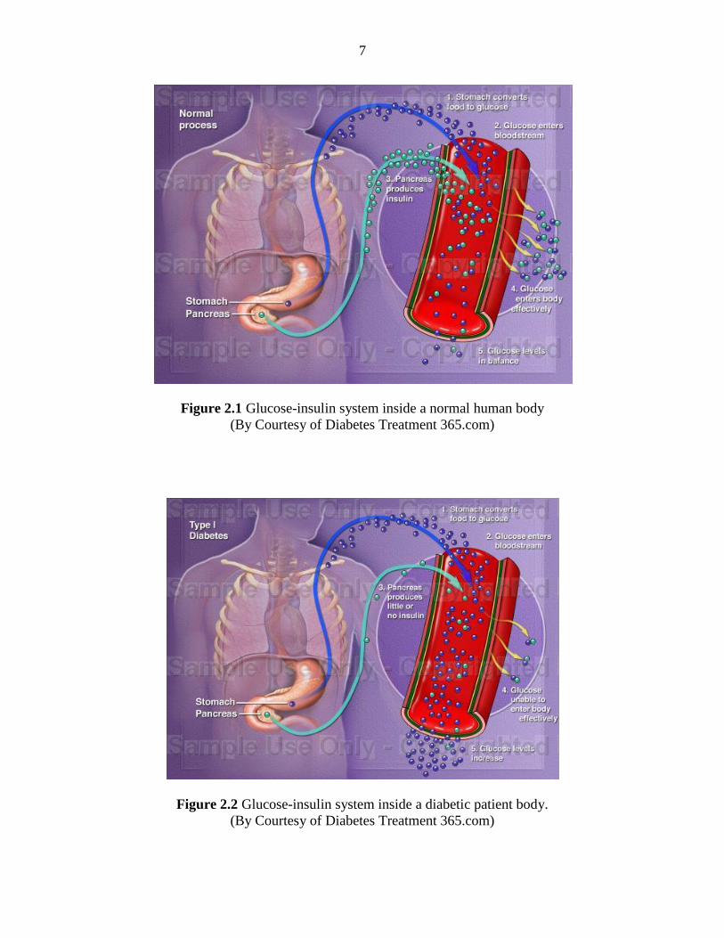
Normally, blood glucose levels are tightly controlled by insulin. The rise in blood sugar level

normally signals special cells in the pancreas, called beta cells, to release the right amount of

insulin to normalize the glucose level in the blood and lower it to the normal level. The glucose-

insulin system inside a normal human body is shown in Figure 2.1, while Figure 2.2 shows the

glucose-insulin system inside a diabetic patient. Typically, the normal range of the glucose level

in a normal individual should fall between 3.9 – 7.7 millimole/liter, (mmol/l), or in metric system

70 – 140 milligram/deciliter, (mg/dl) [11, 12]. The conversion factor between mmol/l and mg/dl

is given by the following 1 millimole/liter = 18.18 milligram/deciliter

In type „I‟ diabetes, the pancreas undergoes an autoimmune attack by the body itself and

is unable of making insulin. Type „I‟ diabetes is caused by an autoimmune destruction of beta

cells in the pancreas, which leads to an absolute insulin deficiency [13]. Abnormal antibodies

have been found in the majority of patients with type „I‟ diabetes. Antibodies are proteins in the

blood that are part of the body's immune system. The patient with type „I‟ diabetes must rely on

insulin medication or injection for survival. In patients with diabetes, the absence or insufficient

production of insulin causes high glucose. Without the insulin, the glucose remains in the blood,

and the body does not receive fuel for energy. The human body cannot function without insulin.

High glucose is unsafe, and if left untreated, can cause a life–threatening complication known as

diabetic ketoacidosis [14, 15]. Over time, high glucose level can lead to blindness, risk of heart

attack, stroke and possible amputation, nerve damage and kidney failure. Also, diabetes can

complicate pregnancy and put a mother at risk for having a baby with birth defects [16, 17].

7

Figure 2.1 Glucose-insulin system inside a normal human body

(By Courtesy of Diabetes Treatment 365.com)

Figure 2.2 Glucose-insulin system inside a diabetic patient body.

(By Courtesy of Diabetes Treatment 365.com)

8

The normal range of blood glucose concentration should be maintained within narrow

limits throughout the day. The average is 70–140 mg/dl, lower in the morning and higher after

the meals [11, 12].

Person’s

Category

Fasting State Postprandial

Glucose

minimum

value

(mg/dl)

Glucose

maximum

value

(mg/dl)

2-3 hours

after eating

(mg/dl)

Hypoglycemia - < 59 < 60

Early

Hypoglycemia 60 79 60 - 70

Normal 80 100 < 140

Early diabetes 101 126 140-200

Diabetic > 126 - > 200

Table 2.1 Blood glucose levels chart

For most normal persons, the glucose levels are between 80 mg/dl and 100 mg/dl in a fasting

state that occurs when a person has not eaten or drunk anything for at least eight hours. Table 2.1

shows the glucose levels for different people categories with the minimum and maximum value

of the glucose level for each category. After eating, the glucose level rises above the normal level

and should fall back to the original starting point within two to three hours. If the glucose level

does not fall, the person is classified as diabetic or at the early diabetes stage. However, the

glucose level should not fall below 60 mg/dl as this is typically the symptom of hypoglycemia.

There are total of 25.8 million children and adults in the United States, or 8.3% of the

populations have diabetes. Also, there is an estimated 79 million people who are classified as

pre-diabetes patients in the United States. Worldwide there are about 346 million people who are

diabetics. The number is expected to rise to about 438 million by year 2030 [18]. Diabetes is the

9

seventh-leading cause of death worldwide. The condition and its complication cost an estimated

$132 billion annually in the United State alone and about $376 billion worldwide, in terms of

healthcare expenses and lost productivity [19]. Based on the death data, diabetes was a

contributing cause of a total of 231,404 deaths in year 2007 in the United State only [20]. The

following statistics show the rate of heart disease and stroke due to diabetes [18]

In 2004, heart disease was noted on 68% of diabetes-related death certificates among

people aged 65 years or older.

In 2004, stroke was noted on 16% of diabetes-related death certificates among people

aged 65 years or older.

Adults with diabetes have heart disease death rates about two to four times higher than

adults without diabetes.

The risk for stroke is two to four times higher among people with diabetes.

2.3 Automation in Diabetes Control:

Insulin injection is a process in which the level of glucose is monitored to indicate the

adequate amount of insulin. From the technical point of view, it is highly beneficent to

investigate the application of control engineering techniques to automate the infusion of the

insulin. In recent years, many researchers focused on the diabetes problem, and the minimal

model was widely used. The concept and implementation of controlling the insulin infusion for

diabetic individuals has been investigated for a few decades via numerous attempts. Various

types of controllers were designed based on a linear model where the output is adequate in the

neighborhood of the equilibrium points. As an overall remark, the mathematical model that

describes the glucose-insulin system of the human beings is a nonlinear model. It is believed that

10

with deeper investigation of modern nonlinear control techniques, algorithm and methods that

can be applied to studies of diabetes. A closed loop system would accurately manage and

regulate the infusion rate of the insulin to the diabetic patients.

2.4 Nonlinear System Identification:

The knowledge of the mathematical model of the system is an essential task for closed

loop control. The accuracy of the model is required for the system to work properly. Since the

level of glucose inside the human being body changes significantly up or down based on the

amount and the kind of food, it is a nonlinear model. One major key problem in nonlinear system

identification is to estimate the unknown parameters. System identification is the experimental

approach to process modeling. System identification includes the following

Experimental planning

Selection of model structure

Criteria

Parameter estimation

Model validation

Experimental planning is normally to get some experimental data from a medical clinic. The

model structure can be derived based on prior knowledge of the process. When formulating an

identification problem, a criterion is postulated to indicate how well a model fits the

experimental data. By making some statistical assumptions, it is feasible to derive criteria from

probabilistic argument. Estimating the unknown parameters of a mathematical model requires

the input-output data and the class of model. The parameters estimation problem can be

formulated as an optimization problem where the best model is the model that best fits the data

11

according to the given criterion. Nonlinear model is defined as an equation that is nonlinear in

the coefficients or a combination of linear and nonlinear in the coefficients. The nonlinear

estimation is the process of fitting a mathematical model to experimental data to determine

unknown parameters of that model. The parameters are chosen or guessed so that the output of

the model is the best match with respect to the experimental data. Nonlinear models require

iterative methods that start with an initial guess of the unknown parameters. The iteration alters

the current guess until the algorithm converges.

12

CHAPTER 3

DIABETES MATHEMATICAL MODEL

3.1 Introduction:

The minimal model of glucose and insulin was formulated to be the easiest model with

which to deal. This has been shown to be the simplest physiologically based representations that

can respectively account for the observed glucose kinetics when the plasma insulin values are

supplied and for the observed insulin kinetics when the plasma glucose values are supplied. The

minimal model is capable of describing the dynamics of the diabetic patient. The insulin enters

or exits the interstitial insulin compartment at a rate that is proportional to the difference i(t) − ib

of plasma insulin i(t) and the basal insulin level ib [21, 22]. If the level of insulin in the plasma is

below the insulin basal level, insulin exits the interstitial insulin compartment. When the level of

insulin in the plasma is above the insulin basal level, insulin enters the interstitial insulin

compartment. Insulin also can flee the interstitial insulin compartment through another route at a

rate that is proportional to the insulin amount inside the interstitial insulin compartment. On the

other hand, glucose enters or exits the plasma compartment at a rate that is proportional to the

difference g(t) − gb of the plasma glucose level g(t) and the basal glucose level gb. When the

level of glucose in the plasma is below the glucose basal level, the glucose exits the plasma

compartment. When the level of glucose in the plasma is above the glucose basal level, glucose

enters the glucose compartment. Glucose also can flee the plasma compartment through another

route at a rate that is proportional to the glucose amount inside the interstitial insulin

compartment. The normal range of blood glucose concentration should be maintained within

13

narrow limits throughout the day, 70–140 mg/dl, lower in the morning and higher after the meals

[11, 12].

3.2 Minimal Model Structures:

The level of glucose inside the human being body changes significantly in response to

food intake and other physiological and environment conditions. It is necessary to derive

mathematics models to capture such dynamics for control design [11-12, 21-26]. Over the years,

many mathematical models have been developed to describe the dynamic behavior of the human

glucose/insulin system. Such models are highly nonlinear and usually very complex. The most

commonly used and simplified model is the minimal model introduced by Bergman [6, 26-32].

The minimal model consists of a set of three differential equations with unknown parameters.

Since diabetic patients differ dramatically due to variations of their physiology and pathology

characteristics, the parameters of the minimal model are significantly different among patients.

Based on such models, a variety of control technologies have been applied to glucose/insulin

control problems.

The minimal model has been developed and tested on healthy subjects whose insulin is

released by the pancreas depending on the actual blood glucose concentration [21]. The minimal

model consists of two parts [27-29]: the minimal model of glucose disappearance (g and v) and

the minimal model of insulin kinetics (i). The mathematical minimal model is stated below

11

.

bg t P v t g t Pg (3.1)

.

2 3 bi tv t P v t P i (3.2)

.

i t n i t g t h t (3.3)

14

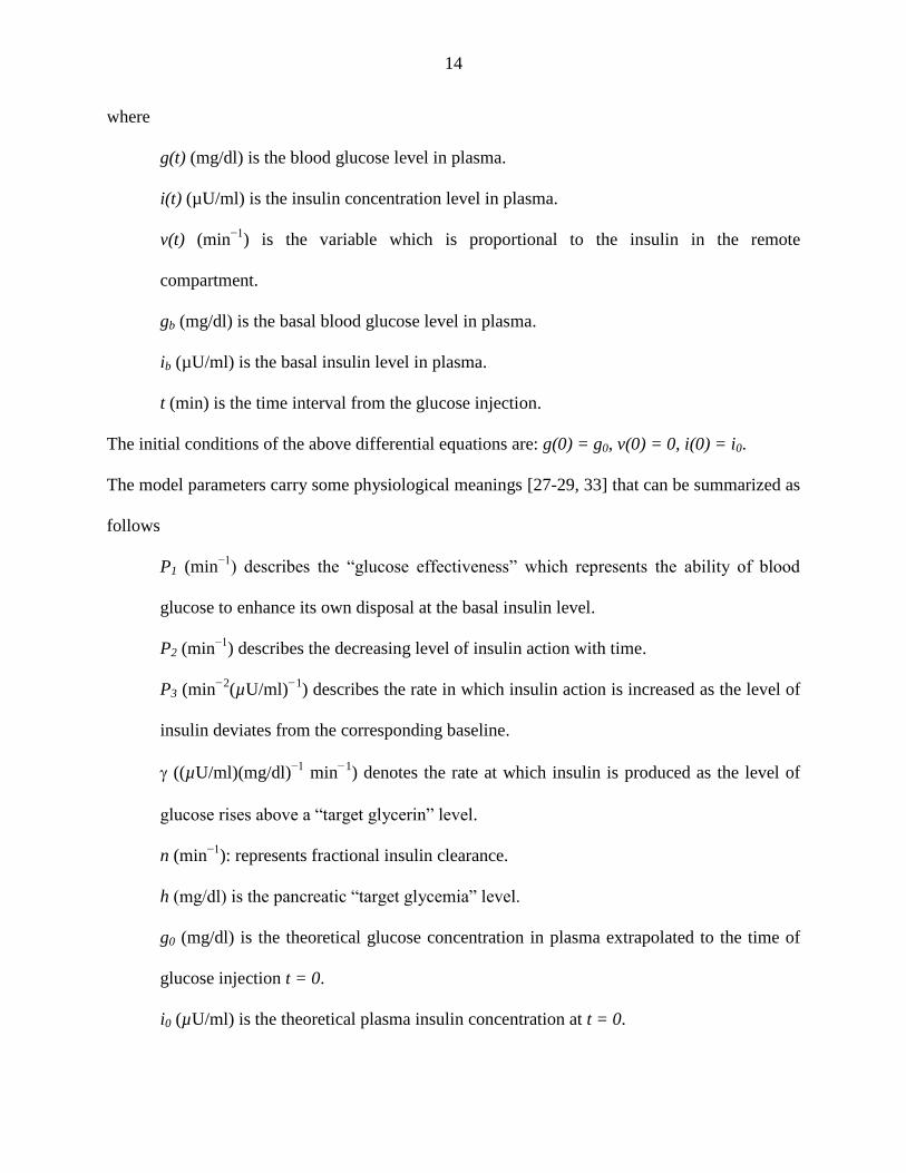
where

g(t) (mg/dl) is the blood glucose level in plasma.

i(t) (µU/ml) is the insulin concentration level in plasma.

v(t) (min−1

) is the variable which is proportional to the insulin in the remote

compartment.

gb (mg/dl) is the basal blood glucose level in plasma.

ib (µU/ml) is the basal insulin level in plasma.

t (min) is the time interval from the glucose injection.

The initial conditions of the above differential equations are: g(0) = g0, v(0) = 0, i(0) = i0.

The model parameters carry some physiological meanings [27-29, 33] that can be summarized as

follows

P1 (min−1

) describes the “glucose effectiveness” which represents the ability of blood

glucose to enhance its own disposal at the basal insulin level.

P2 (min−1

) describes the decreasing level of insulin action with time.

P3 (min−2

(µU/ml)−1

) describes the rate in which insulin action is increased as the level of

insulin deviates from the corresponding baseline.

((µU/ml)(mg/dl)−1

min−1

) denotes the rate at which insulin is produced as the level of

glucose rises above a “target glycerin” level.

n (min−1

): represents fractional insulin clearance.

h (mg/dl) is the pancreatic “target glycemia” level.

g0 (mg/dl) is the theoretical glucose concentration in plasma extrapolated to the time of

glucose injection t = 0.

i0 (µU/ml) is the theoretical plasma insulin concentration at t = 0.

15

µU/ml is the conventional unit to measure the insulin level and has the following conversion

1 micro-unit/milliliter = 6 picomole/liter (1 µU/ml = 6 pmol/l) [34 35].

A fourth differential equation will be added to the set of the minimal model equations to

represent a first-order pump dynamics

. 1( ) ( ) ( )w t w t u t

a (3.4)

where

w(t) is the infusion rate.

u(t) is the input command.

a is time constant of the first-order pump.

3.3 Literature Surveys:

Many methods and techniques have been investigated, tested, and studied for controlling

the glucose level in type „I‟ diabetes patients. Research in this field has always been model-based

and has moved from the development of the structure of a model of glucose and insulin

dynamics stepping towards model parameter estimation and model personalization to each single

patient‟s requirements.

Lynch and Bequette [36] tested the glucose minimal model of Bergman to design a

Model Predictive Control (MPC) to control the glucose level in a diabetic patient. The insulin

secretion term g h t of the differential equation of the minimal model was replaced by

a constant term which makes the infusion of the insulin to be constant and independent of the

glucose level.

16

Fisher [37] used the glucose insulin minimal model of Bergman to design a semi-closed

loop insulin infusion algorithm based on plasma glucose samplings taken over a three hours time

span. The study concentrates on the glucose level and did not take into consideration some

important factors such as free plasma insulin concentration and the rate at which insulin is

produced as the level of glucose rises.

Furler [38] modified the glucose insulin minimal model of Bergman by removing the

insulin secretion and adding insulin antibodies to the model. The algorithm calculates the insulin

infusion rate as a function of the measured plasma glucose concentration. The linear

interpolation was used to find the insulin rate. The algorithm neglected some important

variations in insulin concentration and other model variables. Also, it took more than two hours

to bring the glucose level to the neighborhood of the glucose basal level.

Ibbini, Masadeh and Amer [39] tested the glucose minimal model of Bergman to design a

semi closed-loop optimal control system to control the glucose level in diabetes patients. Also, in

that study, the term t of the minimal model has been eliminated which makes the linearized

version of the minimal model to be a time-invariant system.

3.4 Experimental Data:

A new approach was developed by Bergman [27-29] to compute the pancreatic

responsiveness and insulin sensitivity in the intact organism. This approach uses computer

modeling to investigate the plasma glucose and insulin dynamics during a Frequently Sampled

Intravenous Glucose Tolerance (FSIGT). The FSIGT test was performed after an overnight fast.

An amount of glucose of 0.3g of glucose per 1 kg of patient body weight was injected at t = 0

over a period of time equal to 60 seconds [27-29][40]. The blood samples were taken at regular

17

intervals of time and then analyzed for glucose and insulin content. Glucose was measured in

triplicate by the glucose oxidize technique on an automated analyzer. The coefficient of variation

of a single glucose determination was about ± 1.5%. Insulin was measured in duplicate by

radioimmunoassay, with dextrin-charcoal separation using a human insulin standard. Table 1

shows the FSIGT test data for a normal individual.

Sampling time

(minutes)

Glucose level

(mg/dl)

Insulin level

(µU/ml)

0 92 11

2 350 26

4 287 130

6 251 85

8 240 51

10 216 49

12 211 45

14 205 41

16 196 35

19 192 30

22 172 30

27 163 27

32 142 30

42 124 22

52 105 15

62 92 15

72 84 11

82 77 10

92 82 8

102 81 11

122 82 7

142 82 8

162 85 8

182 90 7

Table 3.1 FSIGT test data for a normal individual.

The plot of the glucose g(t) and the insulin i(t) levels versus time, t, during the FSIGT test are

plotted in Figure 3.1 and 3.2 respectively.

18

Figure 3.1 Glucose level g(t) during the FSIGT test

for a normal individual

Figure 3.2 Insulin level i(t) during the FSIGT test

for a normal individual

0 20 40 60 80 100 120 140 160 180 2000

50

100

150

200

250

300

350

400

time [min]

g(t

) [m

g/d

l]

Experimental Data

Basal Level

0 20 40 60 80 100 120 140 160 180 2000

20

40

60

80

100

120

140

time [min]

Ins

ulin

[m

icro

U/m

l]

Experimental Data

Basal Level

19

CHAPTER 4

SIMULATION OF MINIMAL MODEL

4.1 Introduction:

The implementation of the minimal model can be achieved by using computer simulation

software. Computer simulation is a computer program that attempts to simulate an abstract

model of a particular system. Computer simulations have become a useful part of mathematical

modeling of many natural systems in physics, chemistry, biology, medical, biomedical and

engineering to gain insight into the operation of those systems. Traditionally, the formal

modeling of systems has been via a mathematical model, which attempts to find analytical

solutions to problems which enable the prediction of the behavior of the system from a set of

parameters and initial conditions.

4.2 Simulation of the Glucose Kinetics Model:

Implementation of the minimal model can be achieved by using computer simulation

tools. The mathematical minimal model is stated in chapter 3 and repeated here for convenience

11

.

bg t P v t g t Pg (4.1)

.

2 3 bi tv t P v t P i (4.2)

.

i t n i t g t h t (4.3)

The two differential equations (4.1) and (4.2) correspond to the glucose kinetics are modeled

here by using the MATLAB/Simulink software. In this model, the insulin i(t) is considered as an

20

input and the glucose g(t) as an output. The values of the input i(t) at a time interval are given in

Table 3.1. The simulation diagram of the minimal model for the glucose kinetics is shown in

Figure 4.1. The output of the system, glucose g(t), is shown in Figure 4.2 for a normal individual

with the following parameters [27-29]

P1 = 3.082 x 10-2

P2 = 2.093 x 10-2

P3 = 1.062 x 10-5

g0 = 350

gb = 92

ib = 11

Figure 4.1 Simulation diagram of the glucose kinetics model

g

v

P3(i - ib)

g

i

v.g

dg/dtgb - g P1(gb - g)

P2.v

ib

Scope "g"

Look-Up

Table

1

s

Integrator2

1

sxo

Integrator1

P3

P2

P1

gb

g0

Clock

vdv /dt

21

Figure 4.2 The simulated output g(t) of the glucose kinetics model

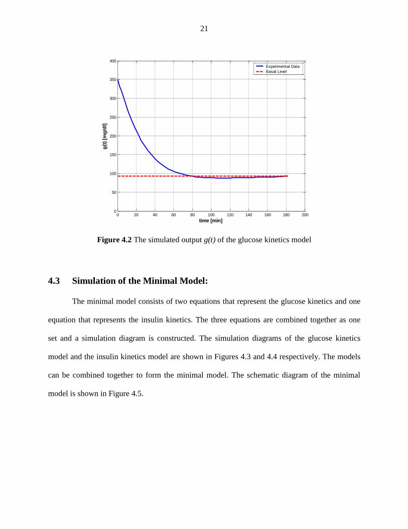
4.3 Simulation of the Minimal Model:

The minimal model consists of two equations that represent the glucose kinetics and one

equation that represents the insulin kinetics. The three equations are combined together as one

set and a simulation diagram is constructed. The simulation diagrams of the glucose kinetics

model and the insulin kinetics model are shown in Figures 4.3 and 4.4 respectively. The models

can be combined together to form the minimal model. The schematic diagram of the minimal

model is shown in Figure 4.5.

0 20 40 60 80 100 120 140 160 180 2000

50

100

150

200

250

300

350

400

time [min]

g(t

) [m

g/d

l]

Experimental Data

Basal Level

22

Figure 4.3 Simulation diagram of minimal model (glucose kinetics part)

Figure 4.4 Simulation diagram of minimal model (insulin kinetics part)

23

Figure 4.5 Simulation diagram of minimal model

The minimal model simulation diagram shown on Figure 4.5 is tested on a normal individual

with the following parameters [29]

P1 = 2.6x10-2

P2 = 2.5x10-2

P3 = 1.25x10-5

gb = 92

ib = 11

g0 = 279

i0 = 363.7

n = 0.287

h = 83.7

= 0.0041

24

The graph of the output of the system, the glucose level g(t), is shown in Figure 4.6. The

glucose level reaches the glucose basal level of a normal individual within 65 minutes. That

observation leads to conclude the minimal model simulation diagram is achieving the goal.

Figure 4.6 Graph of glucose level of the minimal model for normal patient

0 20 40 60 80 100 120 140 160 180 2000

50

100

150

200

250

300

time [min]

g(t

) [m

g/d

l]

g(t)

Basal Level

25

CHAPTER 5

PARAMETERS ESTIMATION

5.1 Introduction:

Parameter estimation is a common problem in many areas of process modeling. The goal

is to determine values of model parameters that provide the best fit to measured data, generally

based on some type of least squares or maximum likelihood criterion. Parameter estimation can

be described as a method that is able to take control of a model running it as many times as it

needs while adjusting its parameters until the discrepancies between selected model outputs and

a set of data or laboratory measurements are reduced to a minimum in the weighted least square

sense.

5.2 Least Squares Parameter Estimation:

The method of least squares assumes that the best-fit curve of a given set of data is the

curve that has the minimal sum of the deviations squared (least squares error) from a given set

of data [42-44]. Assume a set of data given as: 1 1 2 2 3 3 , , , , , ,........, , N Nx y x y x y x y ,

where the independent variable is x and the dependent variable is y . The curve f(x) is the fitting

curve that has the deviation or what is called the error d. The error d is basically the horizontal

(or vertical) distance between the points and the fitted graph. The error d can be defined as the

following

26

1 1 1

2 2 2

3 3 3

= ( )

= ( )

= ( )

= ( )N N N

d y f x

d y f x

d y f x

d y f x

(5.1)

As per the principle of the least square method, the best fitting curve has the following property

2 2 2 2 2

1 2 3

1

+ + + ...... N

N i

i

d d d d d

(5.2)

where the symbol ( ) represents the minimum least square error. Now substituting equation

(5.1) into equation (5.2), we obtain

2

1

( )N

i i

i

y f x

(5.3)

When the function is to the m-th degree polynomial form

2 3

0 1 2 3( ) ..... m

mf x a a x a x a x a x (5.4)

The minimum Least Squares Error becomes

2

1

22 3

0 1 2 3

1

( )

( ..... )

N

i i

i

Nm

i i i i m i

i

y f x

y a a x a x a x a x

(5.5)

The unknown coefficients 0 1 2 3, , , ,....., ma a a a a can be estimated to yield a minimum least

squares error. This can be done by taking the partial derivatives with respect to unknown

coefficients and set the derivative equation to zero as the following

27

2

2 3

0 1 2 3

10 0

2

2 3

0 1 2 3

11 1

2

2 3

0 1 2 3

12 2

( ..... ) 0

( ..... ) 0

( ..... ) 0

Nm

i i i i m i

i

Nm

i i i i m i

i

Nm

i i i i m i

i

y a a x a x a x a xa a

y a a x a x a x a xa a

y a a x a x a x a xa a

2 3

0 1 2 3

( ..... )m

i i i i m i

im m

y a a x a x a x a xa a

2

1

0N

(5.6)

Taking the partial derivative of equation (5.6) yields

2 3

0 1 2 3

10

2 3

0 1 2 3

11

2 3 2

0 1 2 3

12

2 ( ..... ) 0

2 ( ..... ) 0

2 ( ..... ) 0

Nm

i i i i m i

i

Nm

i i i i m i i

i

Nm

i i i i m i i

i

y a a x a x a x a xa

y a a x a x a x a x xa

y a a x a x a x a x xa

2 3

0 1 2 3

2 ( ..... )m m

i i i i m i i

m

y a a x a x a x a x xa

1

0N

i

(5.7)

Equation (5.7) can be rearranged as

2 3

0 1 2 3

1 1

2 3

0 1 2 3

1 1

2 2 2 3

0 1 2 3

1 1

.....

.....

.....

N Nm

i i i i m i

i i

N Nm

i i i i i i m i

i i

N Nm

i i i i i i m i

i i

y a a x a x a x a x

x y x a a x a x a x a x

x y x a a x a x a x a x

2 3

0 1 2 3

1 1

..... N N

m m m

i i i i i i m i

i i

x y x a a x a x a x a x

(5.8)

28

Expanding equation (5.8) as

2

0 1 2

1 1 1 1 1

2 3 1

0 1 2

1 1 1 1 1

2 2 3 4 2

0 1 2

1 1 1 1 1

1

N N N N Nm

i i i m i

i i i i i

N N N N Nm

i i i i i m i

i i i i i

N N N N Nm

i i i i i m i

i i i i i

y a a x a x a x

x y a x a x a x a x

x y a x a x a x a x

1 2 2

0 1 2

1 1 1 1 1

N N N N Nm m m m m

i i i i i m i

i i i i i

x y a x a x a x a x

(5.9)

Writing equation (5.9) in the matrix format

2

1 1 1 1 1

2 3 1

1 1 1 1 1

2 2 3

1 1 1

1

1

N N N N Nm

i i i i

i i i i i

N N N N Nm

i i i i i i

i i i i i

N N N

i i i i

i i i

Nm

i i

i

y x x x

x y x x x x

x y x x

x y

0

1

4 2

1 1

2

1 1 2

1 1 1 1

N Nm

i i

i i

N N N Nm m m m

i i i i mi i i i

a

a

x x

a

x x x x a

(5.10)

The coefficients 0 1 2 3, , , ,....., ma a a a a can be found using the following equation

29

2

1 1 1 10

2 3 1

1 1 1 1

1

2 3 4 2

1 1 1 1

2

1

N N N Nm

i i i

i i i i

N N N Nm

i i i i

i i i i

N N N Nm

i i i i

i i i i

m

x x x

a

x x x x

a

x x x x

a

a

1

1

1

2

1

1 1 2

1 1 1 1 1

N

i

i

N

i i

i

N

i i

i

N N N N Nm m m m m

i i i i i i

i i i i i

y

x y

x y

x x x x x y

(5.11)

5.3 The Levenberg –Marquardt Algorithm:

Nonlinear model is defined as an equation that is nonlinear in the coefficients or a

combination of linear and nonlinear in the coefficients. The nonlinear estimation is the process of

fitting a mathematical model to experimental data to determine unknown parameters of that

model. The parameters can be obtained iteratively to reduce computational complexity. In

general, the nonlinear models are more difficult to fit than linear models because the unknown

parameters or coefficients cannot be estimated using a simple matrix technique that normally is

used to solve linear equations. Nonlinear models require an iterative method that starts with an

initial guess of the unknown parameters. Each iteration updates the current estimate based on

new observation. Suppose there are m base functions 1 2, ,.... mf f f of n parameters 1 2, ,.... np p p .

The functions and the parameters can be represented as follows

1 2

1 2

( , , ..., )

( , , ..., )

T

m

T

n

f f f f

p p p p

(5.12)

The least squares method is to find the values of the unknown parameters 1 2, ,.... np p p for which

the cost function is minimum, i.e.

30

2

1

1 1

2 2

mT

i

i

S p f f f p

(5.13)

The Levenberg-Marquardt algorithm is an iterative technique that seeks the minimum of

a multivariate function that is expressed as the sum of squares of nonlinear real-valued functions

[41]. It has become a standard technique for nonlinear least-squares problems. Levenberg-

Marquardt can be thought of as a combination of steepest descent and the Gauss-Newton

method. When the current solution is far from the correct one, the algorithm behaves like a

steepest descent method which is guaranteed to converge. When the current solution is close to

the correct solution, it becomes a Gauss-Newton method.

The Levenberg-Marquardt algorithm is an iterative procedure. Let x f p be the

parameterized model function. The minimization starts after an initial guess for the parameters

when vector p is provided. The algorithm is locally convergent; namely, it converges when the

initial guess is close to the true values. In each iteration step, the parameter vector p is updated

by a new estimate pp where p is a small correction term that can be determined by a Taylor

Series expansion which leads to the following approximation

p pf p f p J (5.14)

where, J is the Jacobian of f at p

f p

Jp

(5.15)

Levenberg-Marquardt iterative initiates at the starting point p0 and produces a series of vectors

p1, p2, p3, etc, that converge towards a local minimizer p+

of f [45]. At each step, it is required to

find the small correction factor which minimizes the value of

p px f p x f p J

31

That gives the following

ˆp px f p x x J p e J (5.16)

where p is the solution to a linear least squares problem. The minimum is achieved when the

term pJ e is orthogonal to column space J. Based on that, the following can be concluded

( ) 0Tp

J J e (5.17)

equation (5.17) can be rearranged as the following

T Tp

J J J e (5.18)

The Levenberg-Marquardt algorithm solves a slight variation of equation (5.18), which is known

as the augmented normal equation

TpN J e (5.19)

where the diagonal elements of N are computed as Tii ii

N J J for 0 [45], while the

other elements of the matrix N are identical to those of the matrix TJ J . is called the

damping parameter. If the updated parameter vector, pp , where p is computed from

equation (5.19), yields a reduction in the residual value or error e, then the update is valid and the

process repeats with a decreased damping parameter . Otherwise, the damping parameter is

increased and the augmented normal equation (5.19) is solved again. Then the process iterates

until a value of p that reduces error is found. A flow chart that summarizes the least squares

method is shown in Figure 5.1. The MATLAB Software has the Optimization Toolbox which

has a command called Lsqnonlin for this algorithm.

32

Figure 5.1 Flowchart for the least squares method

5.4 Minimal Model Parameters Estimation:

A glucose level test was conducted on two normal individuals that took three hours [27-

28, 40]. The FSIGT test was performed after an overnight fast, an amount of 298 mg/dl of

glucose was injected in the first normal individual. Another amount of 320 mg/dl of glucose was

injected in the second normal individual. The injection starts at t = 0 and lasts for 60 seconds.

Then blood samples were collected from the two individuals and the glucose levels were

measured. The result is shown in tables 5.2. The two individuals have different weight and their

glucose basal level was 94 mg/dl.

Start

Stop

Data

Enter parameters

initial guess

Solve the system and calculate the LSE

Convergence?

Yes No

Compute Jacobian

Matrix

Print

output

Solve for p

Update

parameter

33

Sampling time

During test

(minutes)

Normal Patient #1 Normal Patient #2

Glucose level

(mg/dl)

Glucose level

(mg/dl)

0 94 94

2 298 320

4 284 303

6 272 289

8 253 272

10 248 258

12 235 244

14 217 223

16 208 205

19 205 194

22 191 182

27 172 169

32 164 152

42 141 139

52 132 122

62 120 112

72 116 105

82 108 100

92 106 98

102 104 97

122 105 97

142 109 95

162 107 94

182 110 93

TABLE 5.1 FSIGT test data for a two normal individuals

The mathematical minimal model is stated in chapter 3 and repeated here for convenience

11

.

bg t P v t g t Pg (5.20)

.

2 3 bi tv t P v t P i (5.21)

.

i t n i t g t h t (5.22)

34

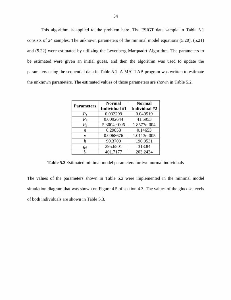
This algorithm is applied to the problem here. The FSIGT data sample in Table 5.1

consists of 24 samples. The unknown parameters of the minimal model equations (5.20), (5.21)

and (5.22) were estimated by utilizing the Levenberg-Marquadrt Algorithm. The parameters to

be estimated were given an initial guess, and then the algorithm was used to update the

parameters using the sequential data in Table 5.1. A MATLAB program was written to estimate

the unknown parameters. The estimated values of those parameters are shown in Table 5.2.

Parameters Normal

Individual #1

Normal

Individual #2

P1 0.032299 0.049519

P2 0.0092644 41.5953

P3 5.3004e-006 1.8577e-004

n 0.29858 0.14653

γ 0.0068676 1.0113e-005

h 90.3709 196.0531

g0 295.6801 318.84

i0 401.7177 203.2434

Table 5.2 Estimated minimal model parameters for two normal individuals

The values of the parameters shown in Table 5.2 were implemented in the minimal model

simulation diagram that was shown on Figure 4.5 of section 4.3. The values of the glucose levels

of both individuals are shown in Table 5.3.

35

Sampling time during

the test (minutes)

Normal individual #1 Normal individual #2

Glucose level (mg/dl) Glucose level (mg/dl)

0 94 94

2 295.6801 318.84

4 282.1308 297.2223

6 268.2993 277.7749

8 254.8580 260.2561

10 242.1020 244.4545

12 230.1353 230.1878

14 218.9702 217.2973

16 208.5776 205.6436

19 198.9116 195.1034

22 185.6659 181.1443

27 173.7810 169.1246

32 156.6159 152.6775

42 142.2917 139.8434

52 120.5167 122.0036

62 105.8327 111.1272

72 96.35277 104.4947

82 90.67314 100.4500

92 87.73594 97.98329

102 86.65621 96.47894

122 86.77255 95.56149

142 89.03143 94.66075

162 92.55181 94.32573

182 95.65837 94.20113

Table 5.3 Simulated glucose levels for two normal individuals

The graphs of both experimental data (Table 5.1) and simulated data (Table 5.3) for normal

individuals #1 and #2 are shown in Figures 5.2 and 5.3 respectively.

36

Figure 5.2 Plot of glucose level g(t) for normal individual #1

Figure 5.3 Plot of glucose level g(t) for normal individual #2

0 20 40 60 80 100 120 140 160 180 2000

50

100

150

200

250

300

350

time [min]

g(t

) [m

g/d

l]

Experimental Data

simulated Data

Basal Level

0 20 40 60 80 100 120 140 160 180 2000

50

100

150

200

250

300

350

time [min]

g(t

) [m

g/d

l]

Experimental Data

simulated Data

Basal Level

37

Figures 5.2 and 5.3 show that the two graphs (experimental and simulated) are close to each

other. That leads to the conclusion that the estimated values of parameters are close to the actual

values.

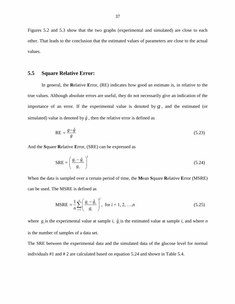
5.5 Square Relative Error:

In general, the Relative Error, (RE) indicates how good an estimate is, in relative to the

true values. Although absolute errors are useful, they do not necessarily give an indication of the

importance of an error. If the experimental value is denoted by g , and the estimated (or

simulated) value is denoted by g , then the relative error is defined as

RE ˆg g

g

(5.23)

And the Square Relative Error, (SRE) can be expressed as

SRE =

2

ˆi i

i

g g

g

(5.24)

When the data is sampled over a certain period of time, the Mean Square Relative Error (MSRE)

can be used. The MSRE is defined as

MSRE

2

1

ˆ1 ni i

i i

g g

n g

, for i = 1, 2, …,n (5.25)

where ig is the experimental value at sample i, ˆig is the estimated value at sample i, and where n

is the number of samples of a data set.

The SRE between the experimental data and the simulated data of the glucose level for normal

individuals #1 and # 2 are calculated based on equation 5.24 and shown in Table 5.4.

38

Normal individual #1

Normal individual #2

Experimental

data, g(t)

Simulated

data, ˆ( )g t SRE

94 94 0

320 318.84 1.314063e-005

303 297.2223 0.0003635986

289 277.7749 0.001508629

272 260.2561 0.001864179

258 244.4545 0.002756472

244 230.1878 0.003204405

223 217.2973 0.0006539557

205 205.6436 9.857924e-006

194 195.1034 3.235126e-005

182 181.1443 2.210359e-005

169 169.1246 5.439401e-007

152 152.6775 1.986409e-005

139 139.8434 3.681781e-005

122 122.0036 8.715616e-010

112 111.1272 6.073247e-005

105 104.4947 2.315634e-005

100 100.4500 2.024906e-005

98 97.98329 2.909034e-008

97 96.47894 2.88559e-005

97 95.56149 0.0002199282

95 94.66075 1.275242e-005

94 94.32573 1.200794e-005

93 94.20113 0.0001668063

Table 5.4 SRE data for between the experimental and simulated glucose level for

normal individuals #1 and #2

Experimental

data, g(t)

Simulated

data, ˆ( )g t SRE

94 94 0

298 295.6801 6.060466e-005

284 282.1308 4.3317e-005

272 268.2993 0.0001851148

253 254.8580 5.393524e-005

248 242.1020 0.0005656016

235 230.1353 0.0004285321

217 218.9702 8.243416e-005

208 208.5776 7.710311e-006

205 198.9116 0.0008820624

191 185.6659 0.0007799362

172 173.7810 0.0001072176

164 156.6159 0.002027272

141 142.2917 8.391868e-005

132 120.5167 0.007568141

120 105.8327 0.01393832

116 96.35277 0.0286871

108 90.67314 0.02573902

106 87.73594 0.02968814

104 86.65621 0.02781129

105 86.77255 0.03013514

109 89.03143 0.03356148

107 92.55181 0.01823304

110 95.65837 0.01699855

39

The graphs of the SRE for both individuals are show in the figures below

Figure 5.4 Plot of SRE for normal individual #1

Figure 5.5 Plot of SRE for normal individual #2

0 20 40 60 80 100 120 140 160 180 200-0.1

-0.08

-0.06

-0.04

-0.02

0

0.02

0.04

0.06

0.08

0.1

time [min]

SR

E

0 20 40 60 80 100 120 140 160 180 200-0.25

-0.2

-0.15

-0.1

-0.05

0

0.05

0.1

0.15

0.2

0.25

time [min]

SR

E

40

Normally, the Mean Square Relative Error is expressed in percentage format. As per equation

(5.25), the percentages MSRE for both individuals are listed below

The percentage MSRE for individual # 1 = 1.79%.

The percentage MSRE for individual # 2 = 0.0149%.

41

CHAPTER 6

PROPOSED MATHEMATICAL

MODEL AND IMPLEMENTATION

6.1 Introduction:

As stated in the previous chapters, the proposed mathematical model consists of three

differential equations that describe the dynamic of a diabetic patient known as minimal model,

and a fourth differential equation that represents a first order infusion pump „P‟. The role of

pump „P‟ is to inject the insulin into the system when the glucose level goes above the normal

basal level.

6.2 Proposed Mathematical Model Analysis:

The differential equation represents the first order infusion pump „P‟ is represented

schematically in Figure 6.1

Figure 6.1 Block diagram of the infusion pump

The dynamic of the first order infusion pump is represented by the following equation

1

( )1

P sas

(6.1)

where “a” is the pump constant.

The relation between the input of the pump and its output can be written as

= w Pu (6.2)

First order

pump, P Input u Output w

42

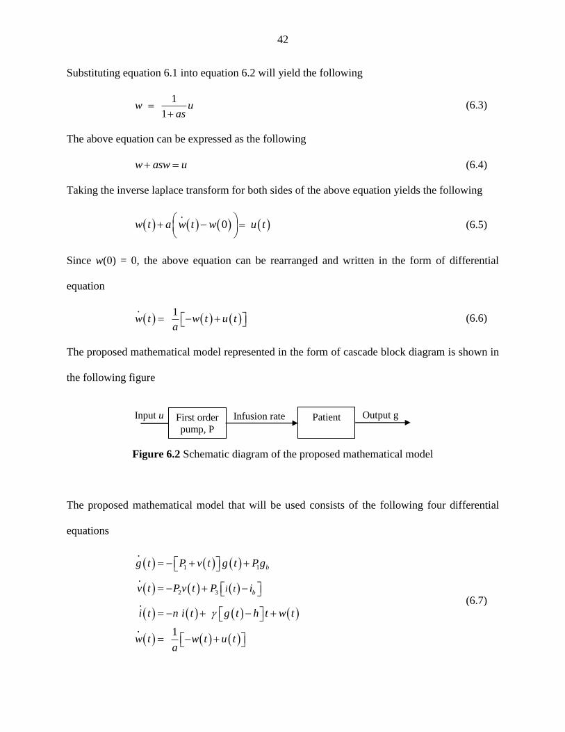
Substituting equation 6.1 into equation 6.2 will yield the following

1

1

w uas

(6.3)

The above equation can be expressed as the following

w asw u (6.4)

Taking the inverse laplace transform for both sides of the above equation yields the following

.

0 w t a w t w u t

(6.5)

Since w(0) = 0, the above equation can be rearranged and written in the form of differential

equation

. 1

w t w t u ta

(6.6)

The proposed mathematical model represented in the form of cascade block diagram is shown in

the following figure

Figure 6.2 Schematic diagram of the proposed mathematical model

The proposed mathematical model that will be used consists of the following four differential

equations

1

2

1

3

.

.

.

. 1

b

b

i t

g t P v t g t Pg

v t P v t P i

i t n i t g t h t w t

w t w t u ta

(6.7)

Input u Infusion rate

w

Output g First order

pump, P

Patient

43

The simulation diagram of the glucose kinetics model is shown in Figure 4.3 in chapter 4. The

simulation diagram of the insulin kinetics model with the first order infusion part is shown in

Figure 6.3.

Figure 6.3 Insulin kinetics simulation diagram with first order infusion pump

The initial conditions of the above four differential equations are

g(0) = g0, v(0) = 0, i(0) = i0, u(0) = 0.

Define the following

1 2 3 4( ) , ( ) , ( ) , ( )x t g t x t v t x t i t x t w t

Then equation 6.7 can be rearranged as

44

1 1 1 2 1

2 2 2 3 3

3 1 3 4

4 4

1

3

.

.

.

. 1 1

b

bx t Px t x t x t Pg

x t P x t P x t Pi

x t nx t nx t x t ht

x t x t u ta a

(6.8)

6.3 Linearization Overview:

Most components that are found in physical systems have nonlinear characteristics. In

practice, some devices have moderate nonlinear characteristics, or nonlinear properties, that

would occur if they were driven into certain operating regions. For these devices, the modeling

by linear system give quite accurate analytical results over a relatively wide range of operating

conditions. When a nonlinear system is linearized at an operating point, the linear model may

contain time-variant elements [45]. If we are interested in values of the function close to some

point, then often we can replace the given function by its first Taylor polynomial, which is a

linear function. That is why the first Taylor polynomial is often called the local linearization. The

use of linearization makes it possible to use tools for studying linear systems to analyze the

behavior of a nonlinear function near a given point. The linearization of a function is the first

order term of its Taylor expansion around the point of interest. To study the behavior of a

nonlinear dynamical system near an equilibrium point, we can linearize the system.

The following is a brief discussion of the linearization of nonlinear first order equations

by using the Taylor Series expansion and the Jacobian Matrix. Consider the following first order

nonlinear equations

45

1 1 2 3 1 2 3

2 1 2 3 1 2 3

3 1 2 3 1 2 3

1 2 3 1 2 3

1

2

3

. , , , ...... , , , , ......

. , , , ...... , , , , ......

. , , , ...... , , , , ......

. , , , ...... , , , , ...

n n

n n

n n

m nn

x f x x x x u u u u

x f x x x x u u u u

x f x x x x u u u u

x f x x x x u u u

... nu

(6.9)

The above equation can be represented in the vector format as shown below

.

,x f x u (6.10)

where

1

1 12

2 2

33 3

.

.

..,

.n n

n

x

x ux

x u

xx x x and u u

x u

x

(6.11)

The Taylor Series expansion of equation (6.10) is

0 1 0 1 0 + + + h.o.tf x f a x x b u u (6.12)

where

0 0

0 0

0 0

1

,

1

,

0 = ,

,

,

x x u u

x x u u

f f x u

df x ua

dx

df x ub

du

46

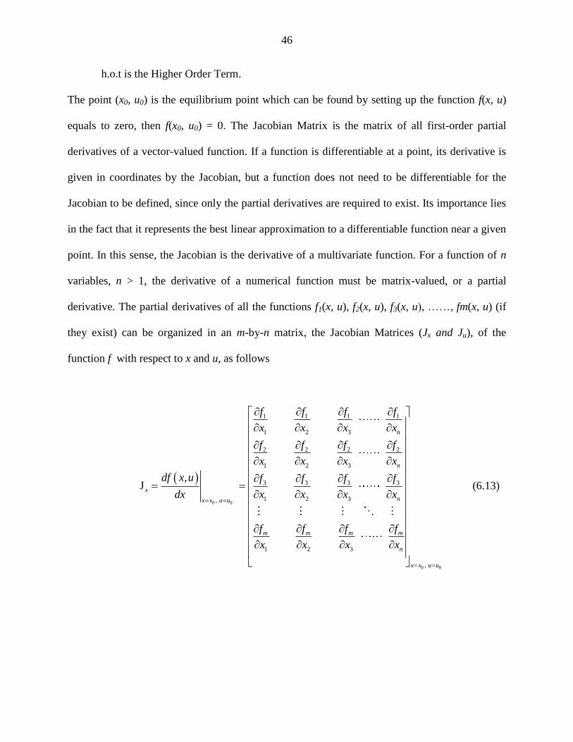
h.o.t is the Higher Order Term.

The point (x0, u0) is the equilibrium point which can be found by setting up the function f(x, u)

equals to zero, then f(x0, u0) = 0. The Jacobian Matrix is the matrix of all first-order partial

derivatives of a vector-valued function. If a function is differentiable at a point, its derivative is

given in coordinates by the Jacobian, but a function does not need to be differentiable for the

Jacobian to be defined, since only the partial derivatives are required to exist. Its importance lies

in the fact that it represents the best linear approximation to a differentiable function near a given

point. In this sense, the Jacobian is the derivative of a multivariate function. For a function of n

variables, n > 1, the derivative of a numerical function must be matrix-valued, or a partial

derivative. The partial derivatives of all the functions f1(x, u), f2(x, u), f3(x, u), ……, fm(x, u) (if

they exist) can be organized in an m-by-n matrix, the Jacobian Matrices (Jx and Ju), of the

function f with respect to x and u, as follows

0 0

1 1 1 1

1 2 3

2 2 2 2

1 2 3

3 3 3 3

1 2 3,

, J

n

n

x

nx x u u

f f f f

x x x x

f f f f

x x x x

df x u f f f f

dx x x x x

f

0 0

1 2 3

,

m m m m

n

x x u u

f f f

x x x x

(6.13)

47

0 0

1 1 1 1

1 2 3

2 2 2 2

1 2 3

3 3 3 3

1 2 3,

, J

n

n

u

nx x u u

f f f f

u u u u

f f f f

u u u u

df x u f f f f

du u u u u

f

0 0

1 2 3

,

m m m m

n

x x u u

f f f

u u u u

(6.14)

The linearized form of the nonlinear system can be written in the state space form as the

following

.

x ux J x J u (6.15)

6.4 Proposed Mathematical Model Linearization:

The proposed mathematical model is a nonlinear model due to the presence of the term

x1(t)x2(t) which is a nonlinear term. The Jacobian Matrices (Jx and Ju) are calculated by

differentiating equation (6.8) with respect to the state variables x1, x2, x3, x4 and the input u, and

substitute in the equations (6.13) and (6.12) we get the following

0 0

1 2 1

2 3

,

0 0

0 0

J 0 1

1 0 0 0

x

x x u u

P x x

P P

t n

a

and

0 0,

0

0

J 0

1

u

x x u ua

(6.16)

where the point (x0, u0) is the equilibrium point. The equilibrium point can be calculated by

setting the state equation to zero and solve as shown below

1 10 10 20 1 0bPx x x Pg (6.17)

48

2 20 3 30 3 0bP x P x Pi (6.18)

10 30 40 0tx nx ht x (6.19)

40 0

1 10x u

a a (6.20)

where, x10, x20, x30, x40 and u0 are the values of the state variables and the input at the operating

point (i.e. the equilibrium point).

At the equilibrium point, u0 = 0, then equation (6.20) becomes as 40

10x

a , that gives

x40 = 0 (6.21)

Substituting the value of x40 in equation (6.19) results 10 30 0tx nx ht and

10

30

x h tx

n

(6.22)

The value of X30 can be substituted in equation (6.18) as 10

2 20 3 3 0b

x h tP x P Pi

n

to

obtain

3 10 3 320

2 2 2

bP tx P th Pix

P n P n P

(6.23)

Now, by substituting the value of x20 in equation (6.17), we have

23 3 3

10 1 10 1

2 2 2

0bb

P t P th Pix P x Pg

P n P n P

(6.24)

The above equation is a 2nd

order equation of the form ax2 + bx + c = 0 and can be solved by

using the quadratic formula

2

10

4

2

b b acx

a

(6.25)

49

where 3 3 31 1

2 2 2

, , .bb

P t P th Pia b P c Pg

P n P n P

There are two possible values (solutions) of x10. Since x20 and x30 are expressed in term of x10,

there will be two values for each. Based on that, the controllability test will be studied to check

which value of x10 is accepted.

6.5 Proposed Mathematical Model Experimental Study:

The following are the parameters values of the mathematical minimal model that

represent the dynamic of a diabetic patient [27-29]

P1 = 0

P2 = 0.81/100

P3 = 4.01/1000000

i0 = 192

g0 = 337

= 2.4/1000

h = 93

n = 0.23

gb = 99

ib = 8

a = 2

These values of the parameters are substituted in the patient dynamic system and the simulation

is run using the minimal model simulation diagram that is shown in Figure 4.5. The result of the

simulation is shown in Figure 6.4.

50

By examining Figure 6.4, it can be clearly seen that the glucose level does not come

down to the basal level after injecting an amount of 337 mg/dl of glucose inside a diabetic

patient. The graph shows that the level of glucose inside a diabetic patient decreases for almost

the first 100 minutes and starts increasing afterward and reaches the value of almost 310 mg/dl

after 3 hours from the time the glucose was injected [46]. The goal is to lower the value of

glucose inside a diabetic patient to the normal level or at least to the neighborhood of the basal

level.

Figure 6.4 Simulated glucose level g(t) for diabetic patient

6.6 State Space Representations:

The state space method is based on the description of the system equation in terms of n

first order difference equations or differential equations, which may be combined into a first

order vector matrix difference equations or differential equations [47]. Let us define some terms

of the state space system.

0 20 40 60 80 100 120 140 160 180 2000

50

100

150

200

250

300

350

400

time [min]

g(t

) [m

g/d

l]

g(t)

Basal Level

51

State Variables: The variables making up the smallest set of variables that

determine the state of the dynamic system.

State Vector: If n state variables are needed to completely describe the behaviour

of a given system, then the n state variable can be considered the n component if

the vector.

State Space Equation: There are three types of variable that are involved in the

modeling of dynamic systems

i. Input Vector.

ii. Output Vector.

iii. State Variable.

The general form of the state space is defined as

x Ax Bu

y Cx Du

(6.26)

where

x is the state vector.

y is the output vector.

u is the control vector.

A is the state matrix.

B is the control matrix.

C is the output matrix.

D is the direct transmission matrix.

The proposed mathematical model at the equilibrium point (x0, u0) can be written in the state

space form as shown below

52

1 20 10

2 3

0 0 0

0 0 0

0 0 1

11 0 0 0

1 0

P x x

P P

x x ut n

aa

y

0 0 x

(6.27)

where u is the input and y is the output of the system. The data of a diabetic person shown in

section 6.5 was used, and the equilibrium point (x0, u0) was calculated as time varied from t = 1

min to t = 182 min. The two values for x10 were calculated using equation (6.25), and it was

found that only one of these values, (the one obtained from the 2 4

2

b b ac

a

), makes the

system controllable; hence, only this value is used in the subsequent development.

6.7 Transfer Function and State Space Representations:

A dynamic system can be expressed either in the state space representation or in the

transfer function representation. The transfer function of a continuous time-invariant state space

model can be derived by taking the laplace transform of the sate space equation (see equation

6.26).

The laplace transform of

x Ax Bu

y Cx Du

yields

( ) ( ) ( )

( ) ( ) ( )

sX s AX s BU s

Y s CX s DU s

(6.28)

Solve the above equation for X(s) as

53

1

( ) ( )X s sI A BU s

(6.29)

Substitute X(s) in the oputput of the system as

1( ) ( ) ( )Y s C sI A BU s DU s

(6.30)

Rearrange equation (6.30) yields

1( ) ( )Y s C sI A B D U s

(6.31)

Since the transfer function of a dynamic system is defined as the ratio of the output to the input

of a system, then

1( )

( )( )

Y sG s C sI A B D

U s

(6.32)

54

CHAPTER 7

LOW-COMPLEXITY REGIME-SWITCHING

INSULIN CONTROL OF TYPE ‘I’ DIABETIC PATIENTS

7.1 Overview:

This chapter studies the benefits of using simplified adaptation control strategies in

improving performance of insulin control for type „I‟ diabetic patients. Typical dynamic models

of glucose levels in diabetic patients are nonlinear. Using a linear time-invariant controller based

on an operating condition is a common method to simplify control design. On the other hand,

adaptive control can potentially improve system performance, but it increases control complexity

and may create further stability issues. This research investigates patient model identification and

presents a simplified switching control scheme using PID controllers [46]. By comparing

different switching schemes, it shows that switched PID controllers can improve performance,

but frequent switching is unnecessary. These findings lead to a control strategy that utilizes only

a small number of PID controllers in this scheduled adaptation strategy.

7.2 Introduction to PID Controller:

In the control of any dynamic system, no controller has better reliability than that of the

PID controller. Out of all the control design techniques, the PID controller becomes the most

widely known and used one. There are many different types and design methods for the PID

controller. Since many control systems using PID controller have proven satisfactory, it still has

a wide range of applications in industrial control [48]. According to a survey for process control

55

systems conducted in 1989, more than 90% of the control loops were of the PID type [49]. PID

controller popularity comes from its simplicity and its ability to be used in a wide variety of

processes. PID controller has been an active research topic for many years.

The term PID stands for Proportional, Integral and Derivative. Each one of these letters (P, I, D)

is term in a control algorithm, and each has a special purpose. It is possible to a PI controller, PD

controller or P controller. It has been found from the experimental point of view that the

structure of the PID controller has sufficient flexibility to yield excellent results in many

dynamic applications [50].

7.3 PID Controller Configuration:

A typical structure of a PID control system is shown in figure 7.1. The basic term is the

proportional term, P, which causes a corrective control actuation proportional to the error. The

integral term, I, gives a correction proportional to the integral of the error. This has the positive

feature of ultimately ensuring that sufficient control effort is applied to reduce the tracking error

to zero. However, integral action tends to have a destabilizing effect due to the increased phase

shift. The derivative term, D, gives a predictive capability yielding a control action proportional

to the rate of change of the error. This tends to have a stabilizing effect but often leads to large

control movements due to the amplification of noise by the derivative action. Various empirical

tuning methods can be used to determine the PID parameters for a given application. They

should be considered as a first guess in a search procedure. Attention should also be paid to the

PID structure [50].

56

Figure 7.1 PID controller structure

From the above figure, it can be clearly seen that in a PID controller, the error signal e(t)

is used to generate the proportional, integral, and derivative actions, with the resulting signals

weighted and summed to form the control signal u(t) applied to the plant model. A mathematical

description of the continuous time linear PID controller is

0

t

p i d

de tu t K e t K e d K

dt (7.1)

where, Kp, Ki, Kd, e, and u are proportion gain, integral gain, derivative gain, error, and output of

the PID controller respectively [51].

7.4 The Characteristics of PID Controller:

A proportional controller (Kp) will have the effect of reducing the rise time and will

reduce but never eliminate the steady-state error. An integral control (Ki) will have the effect of

eliminating the steady state-error, but it may make the transient response worse. A derivative

control (Kd) will have the effect of increasing the stability of the system, reducing the overshoot,

and improving the transient response. Effects of each of controllers Kp, Ki and Kd on a closed-

loop system are summarized in Table 7.1 [ 51-53].

57

Performance Specifications Closed-Loop

Response Rise Time Overshoot Settling Time

Steady-State

Error

Kp Decrease Increase Small Change Decrease

Ki Decrease Increase Increase Eliminate

Kd Small Change Decrease Decrease Small Change

Table 7.1 PID performance measurement tuning table

Note that these correlations may not be exactly accurate, because Kp, Ki, and Kd are dependent of

each other. In fact, changing one of these variables can change the effect of the other two. For

this reason, the table should only be used as a reference when you are determining the values for

Kp, Ki and Kd.

The transfer function, Gc(s), of the PID controller can be calculated by taking the laplace

transform of equation (7.1) which is expressed in the time domain. The following table shows

the laplace transform of the PID controller terms

f t F s

u t U s

e t E s

0

t

e d 1

E ss

de t

dt .s E s

Table 7.2 Laplace transform of PID controller terms

58

Equation (7.1) can be written in the s-domain as

1

p i dU s K E s K E s K sE ss

(7.2)

Rearranging equation (7.2) yield

1

p i dU s K K s K s E ss

(7.3)

The transfer function of the PID controller is

( )

( )

ip d

KU sGc s K K s

E s s (7.4)

The gain Kp is the control action that is proportional to the actuating error signal, which is the

difference between the reference input and the feedback signal or the output. The gain Ki is the

control action which is proportional to the integral of the actuating error signal. Finally, the gain

Kd is the control action which is proportional to the derivative of the actuating error signal. With

the integration of all the three actions, the continuous PID can be designed [51].

Equation (7.4) can be rearranged as

2

p d iK s K s KGc s

s

(7.5)

Based in equation (7.5), the PID controller adds one pole at S=0 and two zeros wherever needed.

Normally, the location of the two zeros is where the two slowest poles can be canceled to be able

to get the best result.

7.5 Design of Individual PID Controllers for Diabetic Patient:

When designing a controller, the designer must define the specifications that need to be

achieved by the controller. Normally, the maximum overshoot (Mp) of the system step response

should be small. Commonly, a range between 10% and 20% is acceptable. Also the settling time

59

(ts), is an important factor. The objective here is to design a PID controller so that the closed-loop

system has the following specifications

Small steady state error for a step input.

Less than 10% maximum overshoot, (Mp).

Settling time, (ts), less than 60 minutes.

The damping ratio and the natural frequency n are related to the maximum overshoot and

the settling time by the following relations

2

2

ln

ln1

p

p

M

M

(7.6)

4n

ts

(7.7)

The patient dynamic system with the parameters shown in section 6.5 was expressed in the state

space representation in equation (7.8). For an overshoot less than 10%, a damping ratio must be

greater than 0.59, and a settling time less than 60 minutes implies that n must be greater

than 0.067.

1 20 10

2 3

0 0 0

0 0 0

0 0 1

11 0 0 0

1 0

P x x

P P

x x ut n

aa

y

0 0 x

(7.8)

60

Analyzing equation (7.8), it is obvious that matrix A is time variant while B and C do not change

with time, and they are fixed in all cases as

0

0 and 1 0 0 0

0

0.5

B C

The PID controllers can be designed based on the following operating points t = 1, 20, 40, 60,

90, 120, 150 and 182 minutes.

7.5.1 Design of PID controller at operating point t = 1 minute:

The control design is done by applying the root locus method and then evaluates it by

using the step response. After substituting the numerical values at operating point t = 1 minute,

the matrix A of equation (7.8) becomes

1

0 859.6667 0 0

0 0.0081 0.00000401 0

0.0024 0 0.23 1

0 0

A

0 0.5

The root locus plot can be generated by the following Matlab program (7.1).

MATLAB Program 7.1

Plotting the open loop system Root locus using MATLAB

[num, den] = ss2tf(A,B,C,D];

rlocus(num, den)

axis([–0.6 0.1 –0.5 0.5])

sgrid(0.59,0)

sigrid(0.067)

61

Figure 7.2 Root Locus plot at operating point t = 1 minute

The open loop poles are shown in Figure 7.2. These poles are located at the following location

Pole 1 = – 0.0040 + 0.0045j

Pole 2 = – 0.0040 – 0.0045j

Pole 3 = – 0.2302

Pole 4 = – 0.5

The four poles are stable, but the first two poles are very close to the imaginary axis and hence

represent the slowest dynamics. The controller takes the form

1 2K s z s z

Gc ss

(7.9)

-0.5 -0.4 -0.3 -0.2 -0.1 0 0.1 0.2 0.3-0.5

-0.4

-0.3

-0.2

-0.1

0

0.1

0.2

0.3

0.4

0.5

0.59

0.59 (zeta)*(w) = 0.067

Root Locus

Real Axis

Ima

gin

ary

Axis

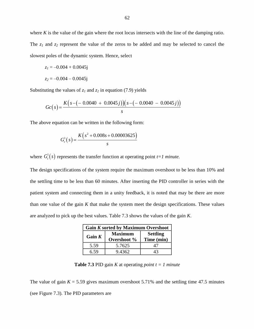
62

where K is the value of the gain where the root locus intersects with the line of the damping ratio.

The z1 and z2 represent the value of the zeros to be added and may be selected to cancel the

slowest poles of the dynamic system. Hence, select

z1 = –0.004 + 0.0045j

z2 = –0.004 – 0.0045j

Substituting the values of z1 and z2 in equation (7.9) yields

0.0040 0.0045 0.0040 0.0045K s j s j

Gc ss

The above equation can be written in the following form:

2

10.008 0.00003625

c

K s sG s

s

where 1

cG s represents the transfer function at operating point t=1 minute.

The design specifications of the system require the maximum overshoot to be less than 10% and

the settling time to be less than 60 minutes. After inserting the PID controller in series with the

patient system and connecting them in a unity feedback, it is noted that may be there are more

than one value of the gain K that make the system meet the design specifications. These values

are analyzed to pick up the best values. Table 7.3 shows the values of the gain K.

Gain K sorted by Maximum Overshoot

Gain K Maximum

Overshoot %

Settling

Time (min)

5.59 5.7625 47

6.59 9.4362 43

Table 7.3 PID gain K at operating point t = 1 minute

The value of gain K = 5.59 gives maximum overshoot 5.71% and the settling time 47.5 minutes

(see Figure 7.3). The PID parameters are

63

4= 0.0444, = 2.0094 10 , 5.59.p i dK K K

Figure 7.3 Unit step response using model at operating point t = 1 minute with K=5.59

7.5.2 Design of PID controller at operating point t = 20 minutes:

After substituting the numerical values at operating point t = 20 minutes, matrix A of

equation (7.8) becomes

20

0 131.33 0 0

0 0.0081 0.00000401 0

0.048 0 0.23 1

0

A

0 0 0.5

The open loop poles of the system are found by the root locus plot to be

Pole 1 = – 0.0038 + 0.0098j

Pole 2 = – 0.0038 – 0.0098j

Step Response

Time(min)

(sec)

Am

plit

ude

0 20 40 60 80 100 120 140 160 180 2000

0.2

0.4

0.6

0.8

1

1.2

1.4

System: G Settling Time (min): 47.5

System: G Peak amplitude: 1.06 Overshoot (%): 5.71

At time (min): 33.6

64

Pole 3 = – 0.2305

Pole 4 = – 0.5

The z1 and z2 represent the value of the zeros to be added and may be selected to cancel the

slowest poles of the dynamic system. Hence, select

z1 = –0.0038 + 0.0098j

z2 = –0.0038 – 0.0098j

Substituting the values of z1 and z2 in equation (7.9) yields

2

200.0076 0.0001

c

K s sG s

s

The same procedure of operating point t = 1 minutes is repeated for operating point t = 20

minutes. Table 7.4 shows the values of the gain K.

Gain K sorted by Maximum Overshoot

Gain K Maximum

Overshoot %

Settling

Time (min)

28.4 1.5633 33

29.4 1.9903 32

30.4 2.4456 48

31.4 2.9223 48

32.4 3.4279 49

33.4 3.9415 48

34.4 4.4716 48

35.4 5.0160 48

36.4 5.5662 47

37.4 6.1187 47

38.4 6.8840 46

39.4 7.2625 45

40.4 7.8303 45

41.4 8.3902 44

42.4 8.9785 44

43.4 9.5369 43

Table 7.4 PID gain K at operating point t = 20 minutes

65

The value of gain K = 28.4 gives maximum overshoot 1.5633% and the settling time 33 minutes.

The PID parameters are

= 0.02160, = 0.0031, 28.4.p i dK K K

7.5.3 Design of PID controller at operating point t = 40 minutes:

At operating point t = 40 minutes, matrix A becomes

40

0 112.17 0 0

0 0.0081 0.00000401 0

0.096 0 0.23 1

0

A

0 0 0.5

The open loop poles of the system are found by the root locus plot to be

Pole 1 = – 0.0036 + 0.00132j

Pole 2 = – 0.0036 – 0.00132j

Pole 3 = – 0.2308

Pole 4 = – 0.5

The z1 and z2 represent the value of the zeros to be added and may be selected to cancel the

slowest poles of the dynamic system. Hence, select

z1 = –0.0036 + 0.00132j

z2 = –0.0036 – 0.00132j

Substituting the values of z1 and z2 in equation (7.9) yields

2

400.0072 0.0002

c

K s sG s

s

The value of gain K = 32.7 gives maximum overshoot 1.2489% and the settling time 34 minutes.

The PID parameters are

66

= 0.02374, = 0.0061, 32.7.p i dK K K

7.5.4 Design of PID controller at operating point t = 60 minutes:

At operating point t = 60 minutes, matrix A becomes

60

0 105.78 0 0

0 0.0081 0.00000401 0

0.144 0 0.23 1

0

A

0 0 0.5

The open loop poles are

Pole 1 = – 0.0035 + 0.00159j

Pole 2 = – 0.0035 – 0.00159j

Pole 3 = – 0.2312

Pole 4 = – 0.5

The PID controller is

2

600.007 0.0003

c

K s sG s

s

The value of gain K = 34.9 gives maximum overshoot 1.3898% and the settling time 34 minutes.

The PID parameters are

= 0.02483, = 0.0095, 35.9.p i dK K K

7.5.5 Design of PID controller at operating point t = 90 minutes:

At operating point t = 90 minutes, matrix A becomes

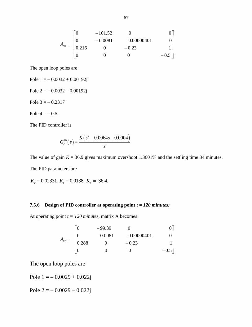
67

90

0 101.52 0 0

0 0.0081 0.00000401 0

0.216 0 0.23 1

0

A

0 0 0.5

The open loop poles are

Pole 1 = – 0.0032 + 0.00192j

Pole 2 = – 0.0032 – 0.00192j

Pole 3 = – 0.2317

Pole 4 = – 0.5

The PID controller is

2

900.0064 0.0004

c

K s sG s

s

The value of gain K = 36.9 gives maximum overshoot 1.3601% and the settling time 34 minutes.

The PID parameters are

= 0.02331, = 0.0138, 36.4.P i dK K K

7.5.6 Design of PID controller at operating point t = 120 minutes:

At operating point t = 120 minutes, matrix A becomes

120

0 99.39 0 0

0 0.0081 0.00000401 0

0.288 0 0.23 1

0

A

0 0 0.5

The open loop poles are

Pole 1 = – 0.0029 + 0.022j

Pole 2 = – 0.0029 – 0.022j

68

Pole 3 = – 0.2322

Pole 4 = – 0.5

The PID controller is

2

1200.0058 0.0005

c

K sG s

s

The value of gain K = 37.9 gives maximum overshoot 1.5325% and the settling time 33 minutes.

The PID parameters are

= 0.02234, = 0.0187, 37.9.P i dK K K

7.5.7 Design of PID controller at operating point t = 150 minutes:

At operating point t = 150 minutes, matrix A becomes

150

0 98.11 0 0

0 0.0081 0.00000401 0

0.36 0 0.23 1

0

A

0 0 0.5

The open loop poles are

Pole 1 = – 0.0027 + 0.0245j

Pole 2 = – 0.0027 – 0.0245j

Pole 3 = – 0.2327

Pole 4 = – 0.5

The PID controller is

2

1500.0054 0.0006

c

K sG s

s

69

The value of gain K = 37.7 gives maximum overshoot 1.2922% and the settling time 34 minutes.

The PID parameters are

= 0.02032, = 0.0229, 37.7.P i dK K K

7.5.8 Design of PID controller at operating point t = 182 minutes:

At operating point t = 182 minutes, matrix A becomes

182

0 97.21 0 0

0 0.0081 0.00000401 0

0.4368 0 0.23 1

0

A

0 0 0.5

The open loop poles are

Pole 1 = – 0.0024 + 0.0269j

Pole 2 = – 0.0024 – 0.0269j

Pole 3 = – 0.2332

Pole 4 = – 0.5

The PID controller is

2

1820.0048 0.0007

c

K sG s

s

The value of gain K = 38.5 gives maximum overshoot 1.3766% and the settling time 34 minutes.

The PID parameters are

= 0.0187, = 0.0281, 38.5.P i dK K K

Non-adaptive PID controllers use a fixed PID controller for the entire control period and

rely on its robustness to maintain control performance [51, 52]. For each individual PID

controller with its transfer function found in the previous subsection at operator points t = 1, 20,

70

40, 60, 90, 120, 150, and 182 minutes, the system is simulated using the simulation diagram

shown in figure 7.4. The results of g(t) are shown below in Figures 7.5 and 7.6.

Figure 7.4 Simulation diagram of the diabetic patient with PID controller

71

Figure 7.5 Simulation of glucose level of PID controllers

at operating points t= 1, 20, 40, and 60 minutes

0 20 40 60 80 100 120 140 160 180 200

0

50

100

150

200

250

300

350

400

time [min]

g(t

) [m

g/d

l]Operating Point t = 1 minute

g(t)

Basal Level

Hypoglycemia

0 20 40 60 80 100 120 140 160 180 200

0

50

100

150

200

250

300

350

400

time [min]

g(t

) [m

g/d

l]

Operating Point t = 20 minutes

g(t)

Basal Level

Hypoglycemia

0 20 40 60 80 100 120 140 160 180 200

0

50

100

150

200

250

300

350

400

time [min]

g(t

) [m

g/d

l]

Operating Point t = 60 minutes

g(t)

Basal Level

Hypoglycemia

0 20 40 60 80 100 120 140 160 180 200

0

50

100

150

200

250

300

350

400

time [min]

g(t

) [m

g/d

l]

Operating Point t = 40 minutes

g(t)

Basal Level

Hypoglycemia

72

Figure 7.6 Simulation of glucose level of PID controllers

at operating points t= 90, 120, 150, and 182 minutes

Under the individual PID controllers, the output g(t), the glucose level, did not really

meet the design specification, and the glucose level is not near or at least in a small

neighborhood of the glucose basal level. The overshoot of the system was too high and beyond

the acceptable level. Also, the settling time was not even close to where it should be as per the

design requirement. And the steady state error was not satisfactory. A new method should be

0 20 40 60 80 100 120 140 160 180 200

0

50

100

150

200

250

300

350

400

time [min]

g(t

) [m

g/d

l]

Operating Point t = 182 minutes

g(t)

Basal Level

Hypoglycemia

0 20 40 60 80 100 120 140 160 180 200

0

50

100

150

200

250

300

350

400

time [min]

g(t

) [m

g/d

l]

Operating Point t = 90 minutes

g(t)

Basal Level

Hypoglycemia

0 20 40 60 80 100 120 140 160 180 200

0

50

100

150

200

250

300

350

400

time [min]

g(t

) [m

g/d

l]

Operating Point t = 120 minutes

g(t)

Basal Level

Hypoglycemia

0 20 40 60 80 100 120 140 160 180 200

0

50

100

150

200

250

300

350

400

time [min]

g(t

) [m

g/d

l]

Operating Point t = 150 minutes

g(t)

Basal Level

Hypoglycemia

73

developed and implemented to meet all the design specifications. This method is explained in

detail in the following section.

7.6 Regime-Switching PID Controller Scheme:

The individual PID controllers could not lower the glucose level g(t) of the patient to the

neighborhood of the glucose basal level. Consequently, we introduce a new Regimes-Switching

control scheme that adapts controllers to meet design specifications. The control scheme consists

of the following items:

One “time clock”.

One “switch case” block.

One “if action case” block.

One “merge” block.

Eight “off–on switches”.

All these blocks are connected together to form the wiring diagram of the Regime-Switching

control scheme. The functions of the Regime-Switching control scheme are detailed in Figures

7.7 and 7.8.

74

Figure 7.7 Regime-Switching Control Scheme wiring diagram

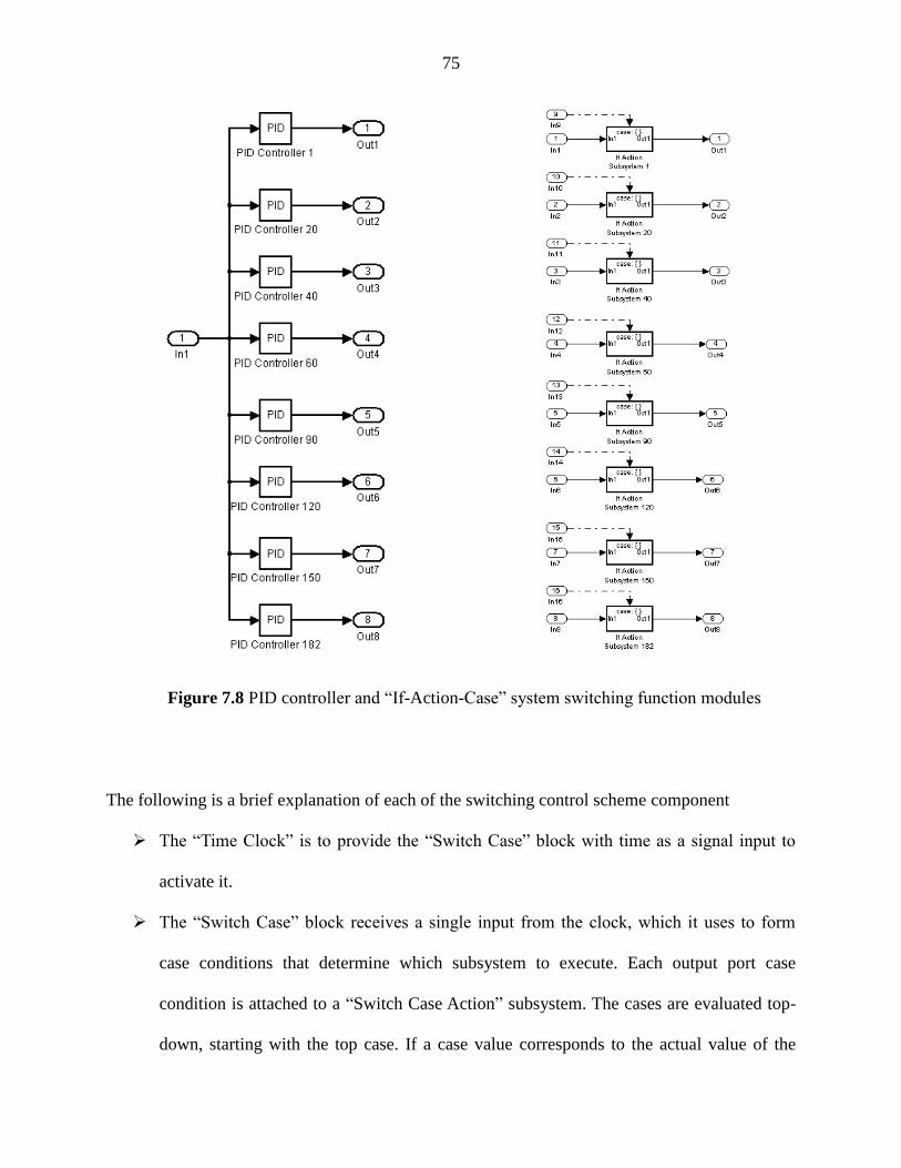
75

Figure 7.8 PID controller and “If-Action-Case” system switching function modules

The following is a brief explanation of each of the switching control scheme component

The “Time Clock” is to provide the “Switch Case” block with time as a signal input to

activate it.

The “Switch Case” block receives a single input from the clock, which it uses to form

case conditions that determine which subsystem to execute. Each output port case

condition is attached to a “Switch Case Action” subsystem. The cases are evaluated top-

down, starting with the top case. If a case value corresponds to the actual value of the

76

input, its “Switch Case Action” subsystem is executed. The “Switch Case” model is

divided into eight time interval zones as shown in Table 7.5.

Zone

number

Time

Interval

(minutes)

1 0 – 1

2 2 – 20

3 21 – 40

4 41 – 60

5 61 – 90

6 91 – 120

7 121 – 150

8 150 – 182

Table 7.5 Regime-Switching time interval

The “If Action Case” block consists of eight “If-Action Subsystems.” The “If-Action

Case” implements Action Subsystems used in the “If-Statement” and switches control

flow statements. Action Subsystems execute their programming in response to the

conditional outputs of an “If-Statement” or “Switch Case” block. A schematic diagram of

the “If Action Case” block is shown in Figure 7.8.

The “Merge” block combines its inputs into a single output line whose value at any time

is equal to the most recently computed output of its driving blocks. The number of inputs

can be specified by setting the block's inputs parameter.

The “Off-On Switches” are Cut-Off switches to turn the PID controllers OFF or ON for

testing purposes.

The “PID Controller System” contains eight PID at operating points t = 1, 20, 40, 60, 90,

120, 150, and 182 minutes.

77

In general, when the time clock is running, it feeds the “Switch Case” block with an input

signal which in turn switches on the “If-Action Case” block as per the time interval that was

specified in Table 7.5. Based on the status of the “If-Action Case”, a specific PID controller will

be turned on and executed to control the output of the system.

For zone 1, the time interval is between 0-1 minute. During this period of time the

“Switch Case” is enabling input “In9” of the “If-Action Case”. When input “In9” is enabled, it

will only execute the input “In1” to the output “Out1”. The input “In1” is connected to the first

PID Controller. That means only the first PID Controller (PID Controller 1) is working. At the

end of the first minute, the “Switch Case” will switch to zone 2 which runs from the beginning of

the minute number 2 and will last until the end of the minute number 20. During this period of

time, the “Switch Case” is enabling input “In10” of the “If-Action Case”. When input “In10” is

enabled, it will only execute the input “In2” to the output “Out2”. The input “In2” is connected

to the second PID Controller. That means only the second PID Controller (PID Controller 20) is

working. The same procedure will be followed until the “Switch Case” switches between the

eight time zones that were specified in Table 7.5. In turn, the PID Controllers will be executed

based on the status of the “If-Action Case”.

The Regime-Switching Control Scheme shown in Figure 7.7 was simulated with all the

PID controllers executed (connected to the circuit). The output g(t) of the system is shown in

Figure 7.9. It can be clearly seen that the PID controllers are able to bring the glucose level from

337 mg/dl to the basal level (99 mg/dl) within 40 minutes. But in about 70 minutes, the value of

the glucose starts going below the basal level, and it went further below the minimum value of

the glucose level. In this case, the person will be classified as a patient with hypoglycemia (low

sugar), and that is not acceptable.

78

Figure 7.9 Plot of glucose level g(t) when all PID controllers are executed

The Regime-Switching Control Scheme was simulated in which all the PID controllers

are executed except the eighth PID controller 182CG . The graph of the output g(t) of the system is

shown in Figure 7.10. It can be seen that the same problem still exists. Again in this case, the

person will be classified as a patient with hypoglycemia.

0 20 40 60 80 100 120 140 160 180 200

0

50

100

150

200

250

300

350

400

time [min]

g(t

) [m

g/d

l]

g(t)

Basal Level

Hypoglycemia

79

Figure 7.10 Plot of glucose level g(t) when all PID controllers except

controller 182

cG are executed

The same procedure was repeated but with all the PID controllers executed except the

PID controllers 150

CG and 182

CG with the graph of the output g(t) shown in Figure 7.11; and

excluding 120

CG , 150

CG , and 182

CG with the simulation result of the output g(t) shown Figure 7.12.

Again, the glucose levels are still below the minimum value and in both cases, the person will be

classified as a patient with hypoglycemia.

0 20 40 60 80 100 120 140 160 180 200

0

50

100

150

200

250

300

350

400

time [min]

g(t

) [m

g/d

l]

g(t)

Basal Level

Hypoglycemia

80

Figure 7.11 Plot of glucose level g(t) when all PID Controllers except

controllers 150

cG and 182

cG are executed

Figure 7.12 Plot of glucose level g(t) when all PID controllers except

controllers 120

cG , 150

cG and 182

cG are executed

0 20 40 60 80 100 120 140 160 180 200

0

50

100

150

200

250

300

350

400

time [min]

g(t

) [m

g/d

l]

g(t)

Basal Level

Hypoglycemia

0 20 40 60 80 100 120 140 160 180 200

0

50

100

150

200

250

300

350

400

time [min]

g(t

) [m

g/d

l]

g(t)

Basal Level

Hypoglycemia

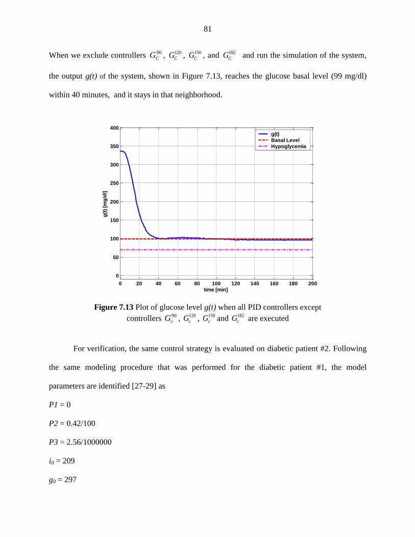
81

When we exclude controllers 90

CG , 120

CG , 150

CG , and 182

CG and run the simulation of the system,

the output g(t) of the system, shown in Figure 7.13, reaches the glucose basal level (99 mg/dl)

within 40 minutes, and it stays in that neighborhood.

Figure 7.13 Plot of glucose level g(t) when all PID controllers except

controllers 90

cG , 120

cG , 150

cG and 182

cG are executed

For verification, the same control strategy is evaluated on diabetic patient #2. Following

the same modeling procedure that was performed for the diabetic patient #1, the model

parameters are identified [27-29] as

P1 = 0

P2 = 0.42/100

P3 = 2.56/1000000

i0 = 209

g0 = 297

0 20 40 60 80 100 120 140 160 180 200

0

50

100

150

200

250

300

350

400

time [min]

g(t

) [m

g/d

l]

g(t)

Basal Level

Hypoglycemia

82

= 3.72/1000

h = 154

n = 0.22

a = 2

gb = 100

ib = 8

Without the Regime-Switching Control Scheme, the above data was implemented in

model simulation. The output of the simulation diagram is shown in Figure 7.14, which shows

that without proper control, the glucose level does not come down to the basal level after

injecting an amount of 297 mg/dl of glucose inside a diabetic patient. The level of the glucose

inside a diabetic patient decreases for the first 120 minutes and starts increasing afterward where

it reaches the value of about 270 mg/dl after 3 hours from the time the glucose was injected.

Figure 7.14 Plot of glucose level g(t) of diabetic patient #2

without control scheme

0 20 40 60 80 100 120 140 160 180 200

0

50

100

150

200

250

300

350

time [min]

g(t

) [m

g/d

l]

g(t)

Basal Level

83

The same control switching scheme that was performed for diabetic patient #1 is repeated for

diabetic patient #2. The values of the parameters for the first four PID controllers at operating

point t = 1, 20, 40 and 60 minutes are summarized in Table 7.6.

PID Controllers Parameters

Gain PID at

t = 1 min

PID at

t = 20 min

PID at

t = 40 min

PID at

t = 60 min

Kp 0.0412 0.1069 0.0868 0.0768

Ki 2.7402*10- 4

0.0047 0.0086 0.014

Kd 10.1 30.6 33.1 33.6

Table 7.6 Paramters of PID controller for diabetic patient #2

The Regime-Switching Control Scheme was simulated for diabetic patient #2 by using only the

first four PID controllers. The graph of the output of the system is shown in Figure 7.15. The

output g(t) reaches the glucose basal level (100 mg/dl) within 60 minutes, and it stays in that

neighborhood.

84

Figure 7.15 Plot of glucose level g(t) of diabetic patient #2 when all PID

controllers except controllers90

cG , 120

cG , 150

cG and 182

cG are executed

7.7 Conclusion:

Based on the simulation results, although adaptive control can potentially improve

control performance, it is sometimes unnecessary, or even harmful, when switching overly

frequently. Our results show that when the Regime-Switching Control Scheme is limited to the

first four PID controllers, the performance is, in fact, enhanced. This may be related to the fact

that some PID controllers are more robust with respect to the model variations. On the other

hand, in comparison to individual controllers, the Regime-Switching Control Scheme achieves

design specification while all individual controllers fail to deliver the required performance.

0 20 40 60 80 100 120 140 160 180 200

0

50

100

150

200

250

300

350

time [min]

g(t

) [m

g/d

l]

g(t)

Basal Level

Hypoglycemia

85

CHAPTER 8

OBSERVER-BASED STATE FEEDBACK DESIGN

8.1 Introduction:

During the past few decades, biomedical modeling techniques have been applied to

improve performance of diabetes that requires monitoring and control. This research focuses on

designing a state feedback controller with an observer to improve the performance of the insulin

control for type „I‟ diabetic patients [54]. The dynamic model of glucose levels in diabetic

patients is a nonlinear model. Using a linear time invariant controller based on an operating

condition is a common method to simplify control design. This research investigates patient

models and presents a simplified control scheme using observer-based feedback controller.

8.2 Introduction to State Feedback Controller:

The design of the state feedback controller is based on the pole placement method using

the Ackermann‟s Formula, with the assumption that all the state variables are measurable and are

available for feedback. If the system is completely state controllable, then the poles of the closed

loop system may be placed at any desired locations by means of state feedback through an

appropriate state feedback gain matrix. By choosing the gain matrix for the state feedback, it is

possible to force the system to have closed loop poles at the desired location, provided that the

original system is completely state controllable [51].

86

8.3 Design of State Feedback Controller:

The state feedback design can be designed on the basis of the pole placement method. In

the pole placement method, the closed loop poles will be placed at desired locations. While this

is similar to root-locus method used in the PID design, the main difference is that in the root-

locus method, only the dominant closed loop poles will be placed at the desired locations. When

designing a controller by the pole placement method, the designer must define the specifications

that need to be achieved by the controller [51, 53]. The objective is to design a state feedback

controller so that the closed-loop system has the following specifications: a small steady-state

error under a step input; less than 10% overshoot; and a settling time less than 60 minutes [54].

We shall choose the control signal to be [51]

u = – Kx (8.1)

That means that the control signal u is determined by an instantaneous state feedback. Such a

scheme is well known as state feedback. The 1× n matrix K is the state feedback gain matrix.

Substituting equation (8.1) into the state space equation .

x Ax Bu , it becomes

. = – x A BK x (8.2)

The stability and the transient response characteristics are determined by the eigenvalues

of matrix A – BK. The eigenvalues of matrix A – BK are called the regular poles. If these poles

are placed in the left half s plane, then x(t) approaches zero as t approaches infinity [55-57]. The

well known Ackermann‟s Formula is used to determine the value of the matrix K [51]. Let the

desired closed loop poles be

1 2 3 4, , , s s s and s

The desired characteristic equation is

87

1 2 3 4

4 3 2

1 2 3 4 0

sI A BK s s s s

s s s s

(8.3)

Let A A BK and substituting it in equation (8.3)

4 3 2

1 2 3 4 0sI A s s s s (8.4)

The Cayley-Hamilton theorem states that A satisfies its characteristic equation as

4 3 2

1 2 3 4 0A A A A A I (8.5)

The following matrix identities are used to derive Ackermann‟s Formula

22 2

33 3 2 2

44 4 3 2 2 3

=

A BK

I I

A A BK

A A ABK BKA

A A BK A A BK ABKA BKA

A A BK A A BK A BK ABKA BKA BKA

(8.6)

Now substituting equation (8.6) in equation (8.5)

4 3 2 2 3

3 2 2

1

2

2 3 4

4 3 2 2 3

3 2 2

1 1 1 1

2

2 2 2 3 3 4

4 3 2

1 2

=

A A A BK A BK ABKA BKA BKA

A A BK ABKA BKA

A ABK BKA A BK I

A A BK A BK ABKA BKA BKA

A A BK ABKA BKA

A ABK BKA A BK I

A A A

3 4

3 2 2

3 2 2

1 1 1

2 2 3

A I

A BK A BK ABKA BKA

BKA A BK ABKA BKA

ABK BKA BK

(8.7)

88

The minimal polynomial of the matrix A is defined in the equation below

4 3 2

1 2 3 4 A A A A A I (8.8)

After substituting equation (8.8) in equation (8.7) and rearranging its terms as

3 2 2

3 2 2

1 1 1

2 2 3

A A A BK A BK ABKA BKA

BKA A BK ABKA BKA

ABK BKA BK

(8.9)

Since 0A , equation (8.9) can be written as

3 2 2

1 2 3

2 3

1 2 1

A B KA KA KA KA K

AB KA K KA A B K K A B K

(8.10)

Equation (8.10) can be rearranged as

3 2 2

1 2 3

2 3 1 2

1

KA KA KA KA K

KA K KAA B AB A B A B

K K

K

(8.11)

Multiplying both sides of equation (8.11) by1

2 3 B AB A B A B

yields

3 2 2

1 2 3

12 3 1 2

1

KA KA KA KA K

KA K KAB AB A B A B A

K K

K

(8.12)

After multiply both sides of equation (8.12) by 0 0 0 1 , we obtain

89

3 2 2

1 2 3

12 3 1 2

1

0 0 0 1 0 0 0 1

KA KA KA KA K

KA K KAB AB A B A B A

K K

K

(8.13)

Equation (8.13) can be written as

1

2 30 0 0 1 K B AB A B A B A

(8.14)

where the matrix 1 2 3 4 .K K K K K

Equation (8.14) is Ackermann‟s Formula used to find the value of the gain K. The desired poles

of the controller can be determined based on the damping ratio and natural frequency n . The

damping ratio and the natural frequency are related to the maximum overshoot, Mp, and the

settling time, ts, with the following relations [51]

21M ep

and

4ts

n (8.15)

Equation (8.15) can be rearranged to obtain the values of the damping ratio and the natural

frequency n

2

2

ln

ln1

p

p

M

M

, and 4

s

nt

(8.16)

The dominant poles are calculated by

2

1,2 1n nP j (8.17)

and the remaining two poles are chosen as

3,4 1,22P P (8.18)

90

By using the data given in section 6.5 for a diabetic patient with maximum overshoot at 10%,

and settling time at 60 minutes, the damping ratio and the natural frequency n are calculated

by using equation (8.16) as [54, 58]

0.5912, and 0.1128.n

The values of the desired poles can be calculated using equations (8.17) and (8.18)

2

1

2

2

3

4

(0.1128)(0.5912) (0.1128) 1 (0.5912) 0.0667 0.091

(0.1128)(0.5912) (0.1128) 1 (0.5912) 0.0667 0.091

2( 0.0667 0.091) 0.1333 0.1819

2( 0.0667 0.091) 0.1333 0.1819

P j j

P j j

P j j

P j j

Using Ackermann‟s Formula (8.14), the state feedback controllers can be designed based

on the models at different operating points. The following are the models at t = 1, 20, 40, 60, 90,

120, 150 and 182 minutes, and the corresponding feedback controllers. Since B and C do not

change with time, they are fixed in all cases as

0

0 , and 1 0 0 0

0

0.5

B C

The following are the matrix A and corresponding matrix K at certain operating points

t = 1 minute:

1

0 859.6667 0 0

0 0.0081 0.00000401 0

0.0024 0 0.23 1

0 0

A

1

0 0.5

0.4 4702.2 0.1 0.7K

91

t = 20 minutes:

20

0 131.33 0 0

0 0.0081 0.000004010 0

0.048 0 0.23 1

0 0

A

20

0 0.5

2.5 4693.8 0.1 0.7K

t = 40 minutes:

40

0 112.17 0 0

0 0.0081 0.00000401 0

0.096 0 0.23 1

0

A

40

0 0 0.5

2.9 4684.8 0.1 0.7K

t = 60 minutes:

60

0 105.78 0 0

0 0.0081 0.00000401 0

0.1440 0 0.23 1

0 0

A

60

0 0.5

3.0 4675.9 0.1 0.7K

t = 90 minutes:

90

0 101.52 0 0

0 0.0081 0.00000401 0

0.2160 0 0.23 1

0 0

A

90

0 0.5

3.1 4662.5 0.1 0.7K

t = 120 minutes:

120

0 99.39 0 0

0 0.0081 0.00000401 0

0.288 0 0.23 1

0 0

A

120

0 0.5

3.2 4649.1 0.1 0.7K

92

t = 150 minute:

150

0 98.11 0 0

0 0.0081 0.00000401 0

0.36 0 0.23 1

0 0

A

150

0 0.5

3.2 4635.7 0.1 0.7K

t = 182 minute:

182

0 97.21 0 0

0 0.0081 0.00000401 0

0.4368 0 0.23 1

0 0

A

182

0 0.5

3.2 4621.4 0.1 0.7K

As mentioned above, the response of the system to the initial condition should approach

zero as the time t approaches infinity. After plotting the responses to initial condition at time t =

1, 20, 40, 60, 90, 120, 150 and 182 minutes, it was noted that the graphs are very close to each

other, and for that reason, only four graphs (randomly selected) are shown in Figure 8.1.

93

Figure 8.1 Response curves to initial conditions at operating points t = 1, 20, 90 and 182

minutes

8.4 Design of State Observer for Linear System:

When designing a state feedback controller by the pole placement method, it is assumed

that all the state variables are available for feedback. In practice, the state variables may not be

available for feedback. Then we need to estimate the unavailable state variables. The process of

estimating the unmeasured state variables is commonly known as observation. The device that

observes the estimation of the unmeasured state variables is called a state observer. The state

0 20 40 60 80 100 120 140 160 180 200-100

-50

0

50

100

150

200

250

300

350

400

time [min]

g(t

) [m

g/d

l]

t = 20: g(t) response to initial condition

0 20 40 60 80 100 120 140 160 180 200-100

-50

0

50

100

150

200

250

300

350

400

time [min]

g(t

) [m

g/d

l]t = 1: g(t) response to initial condition

0 20 40 60 80 100 120 140 160 180 200-100

-50

0

50

100

150

200

250

300

350

400

time [min]

g(t

) [m

g/d

l]

t = 182: g(t) response to initial condition

0 20 40 60 80 100 120 140 160 180 200-100

-50

0

50

100

150

200

250

300

350

400

time [min]

g(t

) [m

g/d

l]

t = 90: g(t) response to initial condition

94

observer estimates the state variables based on the measurements of the output and control

variables. The concept of observability is an important factor in the design of the state observer.

The observability condition must be satisfied before a state observer can be designed [51]. The

notation (t) is used to denote the observed state vector [59, 60]. The mathematical model of the

observer is basically the same as the plant, except that we include the estimation error to

compensate for inaccuracies in the initial state errors. The mathematical model of the observer is

defined as

.

+ – Cex Ax Bu K y x (8.19)

and the control signal to be

–u Kx (8.20)

where is the estimated state, C is the estimated output and Ke is the observer gain matrix [51].

Substituting equation (8.20) into equation (8.19) gives

.

– – + e ex A K C BK x K y (8.21)

The observed state variable (t) can be used to compute the feedback to the system. Figure 8.2

shows the block diagram of the observer-based state feedback control system.

95

Figure 8.2 Observer-based state feedback control wiring diagram

The design process will be done in two phases. The first phase is to calculate the value of

the feedback gain matrix K, and the second phase is to determine the observer gain matrix Ke.

The value of the matrix Ke is calculated by Ackermann‟s Formula for observers as

1

2

3

0

0

0

1

e

C

CAK A

CA

CA

(8.22)

where the matrix

1 2 3 4 .T

e e e e eK K K K K

Now we need to choose the observer gain Ke. Since we want the dynamics of the observer to be

much faster than the system itself, we need to place the poles at least five times farther to the left

than the dominant poles of the system. The values of the desired poles of the observer are

selected as

96

1

2

3

4

0.3333 0.4548

0.3333 0.4548

0.6667 0.9096

0.6667 0.9096

o

o

o

o

P j

P j

P j

P j

The values of matrices K and Ke at certain operating points are calculated by Ackermann‟s

Formula. The values of matrix K were found in the previous section, and the values of matrix Ke

are shown below

t = 1 minute: t = 20 minutes:

1

1.2620

0.0017

22.4977

58.8582

eK

20

1.2620

0.0109

147.2340

385.2770

eK

t = 40 minutes: t = 60 minutes:

40

1.2620

0.0128

172.3436

451.0869

eK

60

1.2620

0.0135

182.7124

478.3364

eK

t = 90 minutes: t = 120 minutes:

90

1.2620

0.0141

190.3134

498.4084

eK

120

1.2620

0.0144

194.3246

509.0897

eK

97

t = 150 minutes: t = 182 minutes:

150

1.2620

0.0146

196.7916

515.7316

eK

182

1.2620

0.0147

198.5401

520.5064

eK

8.5 Individual Observer-Based State Feedback Controllers:

Non-adaptive observer-based state feedback controllers use a fixed controller for the

entire control period and rely on its robustness to maintain control performance. For each

individual observer-based state feedback controller with its gain matrices K and Ke found in the

previous sections at operating points t = 1, 20, 40, 60, 90, 120, 150 and 182 minutes, the

simulation was performed, and the glucose level for each patient was plotted. Based on the

simulation results, it can be seen that under the individual observer-based state feedback

controllers, the glucose level g(t) reaches the basal level within 60 minutes and stays at that level.

By carefully analyzing the plots of the output, it is clear that the optimal graph is when the

observer-based state feedback controller at operating point t = 20 minutes is used. It was noted

that the graphs are very close to each other, and for that reason, only four graphs (randomly

selected) are shown in Figure 8.3.

98

Figure 8.3 Observer-based state feedback controller output, glucose level g(t)

at operating points t = 1, 20, 90 and 182 minutes

8.6 Observer-Based State Feedback Controller for Nonlinear System:

The design for the linear system that was calculated in sections 8.4 and 8.5 is applied to

the nonlinear system at operating point t = 20 minutes. The simulation diagram of the nonlinear

system that defines the dynamics of the diabetic patient with the observer-based state feedback is

0 20 40 60 80 100 120 140 160 180 200

0

50

100

150

200

250

300

350

400

time [min]

g(t

) [m

g/d

l]

t=182: plot of simulated g(t)

g(t)

Basal Level

0 20 40 60 80 100 120 140 160 180 200

0

50

100

150

200

250

300

350

400

time [min]

g(t

) [m

g/d

l]

t=1: plot of simulated g(t)

g(t)

Basal Level

0 20 40 60 80 100 120 140 160 180 200

0

50

100

150

200

250

300

350

400

time [min]

g(t

) [m

g/d

l]

t=20: plot of simulated g(t)

g(t)

Basal Level

0 20 40 60 80 100 120 140 160 180 200

0

50

100

150

200

250

300

350

400

time [min]

g(t

) [m

g/d

l]

t=90: plot of simulated g(t)

g(t)

Basal Level

99

shown in Figure 8.4. The box labeled “subsystem (patient) 1” contains the nonlinear system of

the diabetic patient. The simulation is performed, and the glucose level g(t) is plotted and shown

in Figure 8.5. It is clear that the glucose level for the nonlinear system has the same high

performance as that of the linear system.

Figure 8.4 Observer-based state feedback control wiring diagram

for nonlinear system

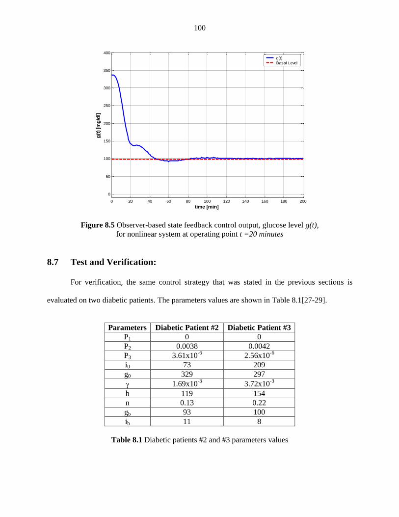
100

Figure 8.5 Observer-based state feedback control output, glucose level g(t),

for nonlinear system at operating point t =20 minutes

8.7 Test and Verification:

For verification, the same control strategy that was stated in the previous sections is

evaluated on two diabetic patients. The parameters values are shown in Table 8.1[27-29].

Parameters Diabetic Patient #2 Diabetic Patient #3

P1 0 0

P2 0.0038 0.0042

P3 3.61x10-6

2.56x10-6

i0 73 209

g0 329 297

1.69x10-3

3.72x10-3

h 119 154

n 0.13 0.22

gb 93 100

ib 11 8

Table 8.1 Diabetic patients #2 and #3 parameters values

0 20 40 60 80 100 120 140 160 180 200

0

50

100

150

200

250

300

350

400

time [min]

g(t

) [m

g/d

l]

g(t)

Basal Level

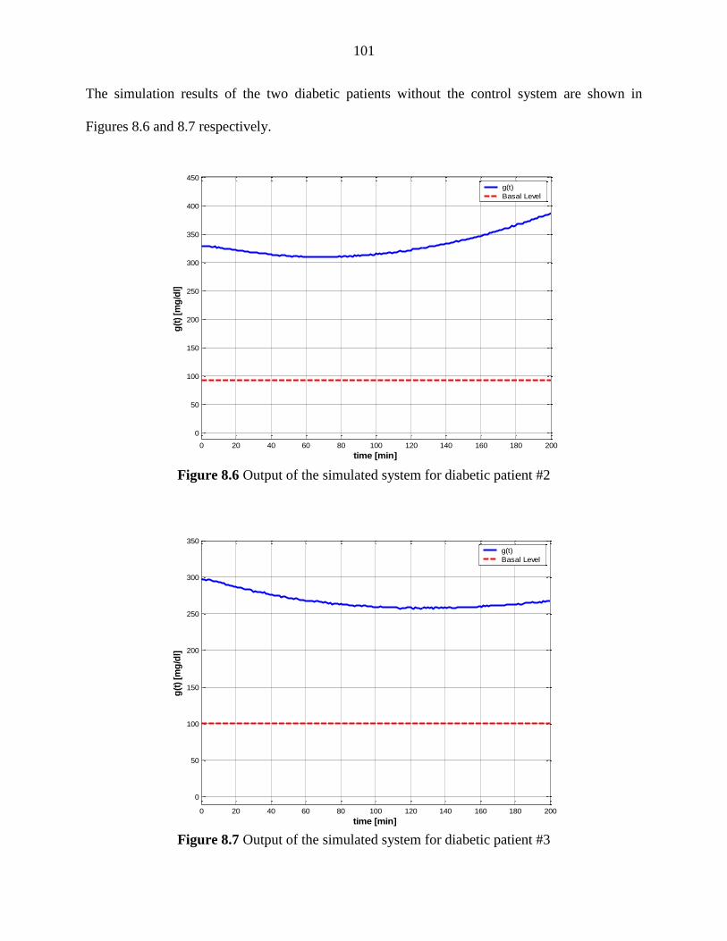
101

The simulation results of the two diabetic patients without the control system are shown in

Figures 8.6 and 8.7 respectively.

Figure 8.6 Output of the simulated system for diabetic patient #2

Figure 8.7 Output of the simulated system for diabetic patient #3

0 20 40 60 80 100 120 140 160 180 200

0

50

100

150

200

250

300

350

400

450

time [min]

g(t

) [m

g/d

l]g(t)

Basal Level

0 20 40 60 80 100 120 140 160 180 200

0

50

100

150

200

250

300

350

time [min]

g(t

) [m

g/d

l]

g(t)

Basal Level

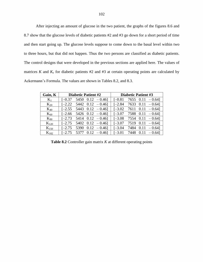
102

After injecting an amount of glucose in the two patient, the graphs of the figures 8.6 and

8.7 show that the glucose levels of diabetic patients #2 and #3 go down for a short period of time

and then start going up. The glucose levels suppose to come down to the basal level within two

to three hours, but that did not happen. Thus the two persons are classified as diabetic patients.

The control designs that were developed in the previous sections are applied here. The values of

matrices K and Ke for diabetic patients #2 and #3 at certain operating points are calculated by

Ackermann‟s Formula. The values are shown in Tables 8.2, and 8.3.

Gain, K Diabetic Patient #2 Diabetic Patient #3

K1 [–0.37 5450 0.12 – 0.46] [–0.81 7655 0.11 – 0.64]

K20 [–2.22 5442 0.12 – 0.46] [–2.84 7633 0.11 – 0.64]

K40 [–2.55 5443 0.12 – 0.46] [–3.02 7611 0.11 – 0.64]

K60 [–2.66 5426 0.12 – 0.46] [–3.07 7588 0.11 – 0.64]

K90 [–2.73 5414 0.12 – 0.46] [–3.08 7554 0.11 – 0.64]

K120 [–2.75 5402 0.12 – 0.46] [–3.07 7519 0.11 – 0.64]

K150 [–2.75 5390 0.12 – 0.46] [–3.04 7484 0.11 – 0.64]

K182 [–2.75 5377 0.12 – 0.46] [–3.01 7448 0.11 – 0.64]

Table 8.2 Controller gain matrix K at different operating points

103

Gain, Ke Patient #2 Patient #3

Ke1

1.3663

  0.0016

  59.4194

  58.2341

1.2759

  0.0023

  55.8586

  126.3840

Ke20

1.3663

0.0096

355.5025

348.4343

1.2759

  0.0081

  197.1173

  446.1300

Ke40

1.3663

0.0111

409.1316

401.0253

1.2759

  0.0087

  211.1101

  477.9540

Ke60

1.3663

0.0117

430.7749

422.2694

1.2759

  0.0089

  216.1793

  489.5925

Ke90

1.3663

0.0121

446.4994

437.7294

1.2759

  0.0090

  219.6407

  497.6747

Ke120

1.3663

0.0123

454.7757

445.8901

1.2759

  0.0091

  221.3588

  501.8151

Ke150

1.3663

0.0124

459.9226

450.9343

1.2759

  0.0092

  222.3589

  504.3313

Ke182

1.3663

0.0125

463.5094

454.5520

1.2759

  0.0092

  223.0300

  506.1187

Table 8.3 Observer gain matrix Ke at different operating points

As in the previous sections, for each individual observer-based state feedback controller with its

gain matrices K and Ke at t = 1, 20, 40, 60, 90, 120, 150 and 182 min, the simulation was

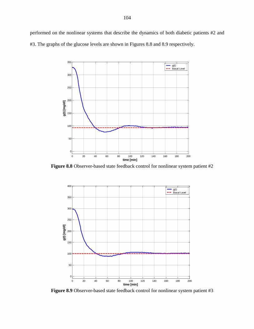
104

performed on the nonlinear systems that describe the dynamics of both diabetic patients #2 and

#3. The graphs of the glucose levels are shown in Figures 8.8 and 8.9 respectively.

Figure 8.8 Observer-based state feedback control for nonlinear system patient #2

Figure 8.9 Observer-based state feedback control for nonlinear system patient #3

0 20 40 60 80 100 120 140 160 180 200

0

50

100

150

200

250

300

350

time [min]

g(t

) [m

g/d

l]g(t)

Basal Level

0 20 40 60 80 100 120 140 160 180 200

0

50

100

150

200

250

300

350

400

time [min]

g(t

) [m

g/d

l]

g(t)

Basal Level

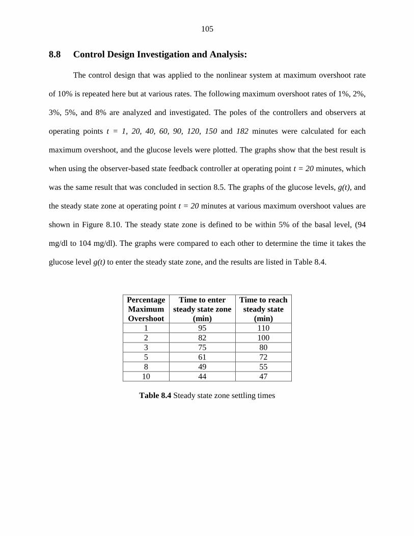
105

8.8 Control Design Investigation and Analysis:

The control design that was applied to the nonlinear system at maximum overshoot rate

of 10% is repeated here but at various rates. The following maximum overshoot rates of 1%, 2%,

3%, 5%, and 8% are analyzed and investigated. The poles of the controllers and observers at

operating points t = 1, 20, 40, 60, 90, 120, 150 and 182 minutes were calculated for each

maximum overshoot, and the glucose levels were plotted. The graphs show that the best result is

when using the observer-based state feedback controller at operating point t = 20 minutes, which

was the same result that was concluded in section 8.5. The graphs of the glucose levels, g(t), and

the steady state zone at operating point t = 20 minutes at various maximum overshoot values are

shown in Figure 8.10. The steady state zone is defined to be within 5% of the basal level, (94

mg/dl to 104 mg/dl). The graphs were compared to each other to determine the time it takes the

glucose level g(t) to enter the steady state zone, and the results are listed in Table 8.4.

Percentage

Maximum

Overshoot

Time to enter

steady state zone

(min)

Time to reach

steady state

(min)

1 95 110

2 82 100

3 75 80

5 61 72

8 49 55

10 44 47

Table 8.4 Steady state zone settling times

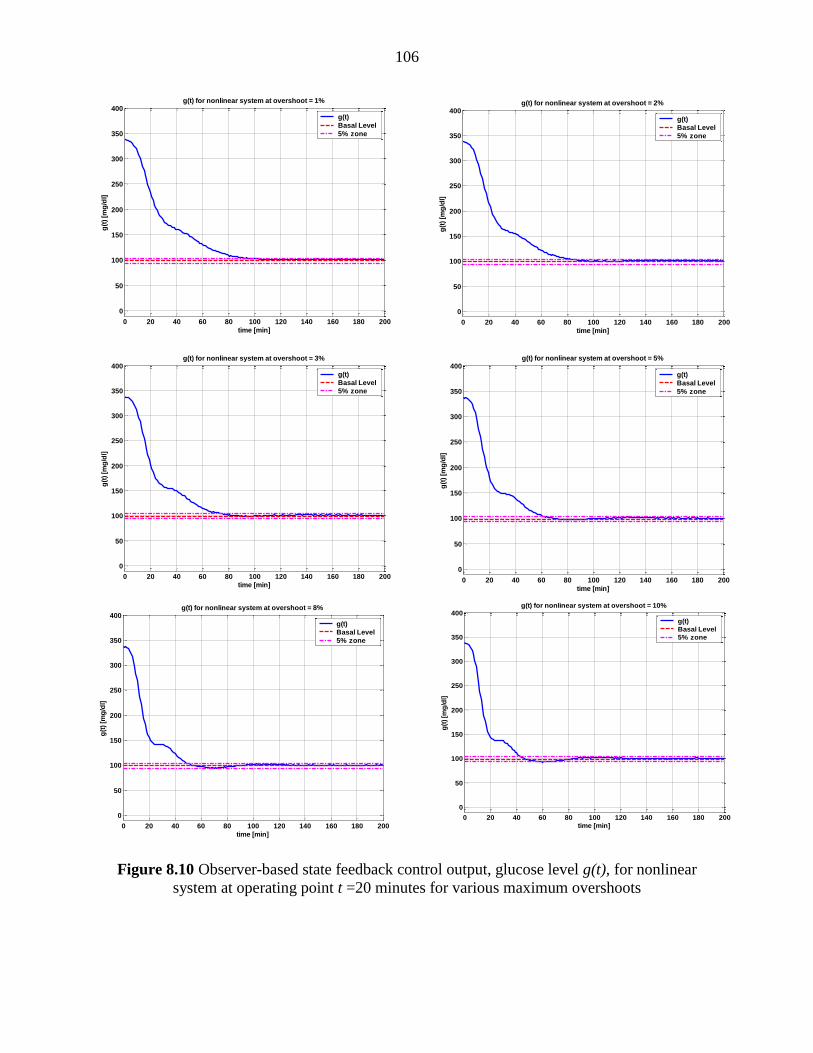
106

Figure 8.10 Observer-based state feedback control output, glucose level g(t), for nonlinear

system at operating point t =20 minutes for various maximum overshoots

0 20 40 60 80 100 120 140 160 180 200

0

50

100

150

200

250

300

350

400

time [min]

g(t

) [m

g/d

l]g(t) for nonlinear system at overshoot = 1%

g(t)

Basal Level

5% zone

0 20 40 60 80 100 120 140 160 180 200

0

50

100

150

200

250

300

350

400

time [min]

g(t

) [m

g/d

l]

g(t) for nonlinear system at overshoot = 2%

g(t)

Basal Level

5% zone

0 20 40 60 80 100 120 140 160 180 200

0

50

100

150

200

250

300

350

400

time [min]

g(t

) [m

g/d

l]

g(t) for nonlinear system at overshoot = 3%

g(t)

Basal Level

5% zone

0 20 40 60 80 100 120 140 160 180 200

0

50

100

150

200

250

300

350

400

time [min]

g(t

) [m

g/d

l]

g(t) for nonlinear system at overshoot = 5%

g(t)

Basal Level

5% zone

0 20 40 60 80 100 120 140 160 180 200

0

50

100

150

200

250

300

350

400

time [min]

g(t

) [m

g/d

l]

g(t) for nonlinear system at overshoot = 8%

g(t)

Basal Level

5% zone

0 20 40 60 80 100 120 140 160 180 200

0

50

100

150

200

250

300

350

400

time [min]

g(t

) [m

g/d

l]

g(t) for nonlinear system at overshoot = 10%

g(t)

Basal Level

5% zone

107

By comparing the result of Table 8.4 and the graphs of Figure 8.10, it is obvious to

conclude when the maximum overshoot is small, the settling time (the time it takes the glucose

level to enter the steady state zone and stay inside that zone) is long. But when the maximum

overshoot is large, the settling time is short.

108

CHAPTER 9

CONCLUSION

A detailed research has been conducted on type “I” diabetic patient to control the glucose

levels and bring it down to the patient basal level. Specific solutions and design have been

developed to improve performance on insulin control for type “I” diabetic patient. The following

gives an executive summary of the contributions and results of this research

In this research, one differential equation that represents a first order infusion pump was

added to the set of the differential equations of the minimal model. The role of the pump

is to inject the required amount of insulin to help the glucose level to come down to basal

level within 2-3 hours after meal.

The Nonlinear Least Squares Method with Levenberg-Marquardt Algorithm was used to

estimate the unknown parameters of the differential equations that describe the dynamic

of diabetic patient.

The simulation diagram of the proposed mathematical model with the estimated

parameters was constructed. The output (glucose) of the simulation diagram was

monitored and recorded. The error between the simulated data and the experimental data

was calculated to be very small.

Typical PID controllers were not sufficient to meet the design specification of the glucose

level control problems. This is mainly due to the nonlinear nature of patient dynamic

models and limited robustness of the PID controllers. An adaptive control that switches

controllers based on operating conditions was developed to potentially enhance the

109

control performance. The regime-switching control scheme was carefully designed to

ensure that the control specifications were met and the number of PID controller was

reduced to four controllers without jeopardizing the enhanced performance of the system.

A simplified control scheme using one observer-based state feedback controller was

presented. The control scheme was able to enhance the performance of the system and

meet the design specifications.

A comparison between the regime-switching control scheme using PID controllers and

the individual observer-based state feedback controller scheme was investigated.

However, the observer-based state feedback control scheme eliminated the switching

strategy that was required in the PID design, and the adaptive control components such as

the “switching case”, the “if action case system”, the “8-intput-1-output merge” block,

and the eight manual cut-off switches were no longer needed. The observer-based state

feedback control scheme reduced the complexity of the control circuit and reduced the

cost to build up the circuit.

The control design was investigated by comparing the results of the control scheme at

various maximum overshoot rates. It was noted that when maximum overshoot was

small, the settling time was longer. But when the maximum overshoot was large, the

settling time was short.

110

REFERENCES

[1] Karam, J. H., Grodsky, G.M., and Forsham, P.H., “Excessive insulin response to glucose

in obese subjects as measured by immunochemical assay”, Diabetes, 1963, vol. 12, pp.

196-204.

[2] Ginsberg, H., Olefsky, J.M., and Reaven, G.M., “Further evidence that insulin resistance

exists in patients with chemical diabetes”, Diabetes, 1974, vol. 23, pp. 674-678.

[3] Reaven, G. M., and Olefsky, J.M., “Relationship between heterogeneity of insulin

responses and insulin resistance in normal subjects and patients with chemical diabetes”,

Diabetologia, 1977, vol. 13, pp. 201-206.

[4] Lerner, R. L., and Porte, D. Jr., “Acute and steady state insulin responses to glucose in

nonobese, diabetic subjects”, J. Clin. Invest., 1972, vol. 51, pp. 1624-1631.

[5] Reaven, G. M., “Insulin-independent diabetes mellitus: metabolic characteristics‟, Metab.

Clin. Exp., 1980, vol. 29, pp. 445-454.

[6] Bergman, R. N., and Cobelli, C., “Minimal modeling, partition analysis, and the

estimation of insulin sensitivity”, Fed. Proc., 1980, vol. 39, pp. 110-115.

[7] Shen, S.W., Reaven, G.M., and Farquhar, J.W., “Comparison of impedance to insulin-

mediated glucose uptake in normal and diabetic subjects”, J. Clin. Invest., 1970, vol. 49,

pp. 2151-2160.

[8] Dua, P., Doyle III F.J., and Pistikopoulos E.N., “Model-based Blood Glucose Control for

Type „I‟ Diabetes via Parametric Programming”, IEEE Trans. Biomed. Eng., 2006, vol.

53, issue , 8, pp. 1478-1491.

[9] Hernjak N., and Doyle III F.J., “Glucose Control Design using Nonlinearity Assessment

Techniques”. AIChE J., 2005, vol. 51, pp.544–554.

111

[10] Radomski, D., Lawrynczuk, M., Marusak, P., and Tatjewski, P., “Modeling of Glucose

Concentration Dynamics for Predictive Control of Insulin Administration”

Biocybernetics and Biomedical Engineering, 2010, vol. 30, number 1, pp. 41–53.

[11] Hovorka R., Canonico V., Chassin L.J., Haueter U., Massi-Benedetti M., Orsini M.

Federici M.O., Pieber T.R., Schaller H.C., Schaupp L., Vering T., and Wilinska M.E.,

“Nonlinear Model Predictive Control of Glucose Concentration in Subjects With Type „I‟

Diabetes”. Physiol. Meas., 2004, vol. 25, pp. 905–920.

[12] Liu, E., and Yuanet, J.M., “DynamicSensitivity and Control Analyses of Metabolic

Insulin Signalling Pathways” IET Systems Biology, 2010, vol. 4, issue 1, pp. 64-81.

[13] Salsai,A., and Muriel, N. F. “A review Types 1 and 2 diabetes mellitus and their

treatement with insulin”, American Journal of Therapeutics, 2006, vol. 13, issue 4,

pp.349-361.

[14] Dunning, T., “Diabetic ketoacidosis – prevention, management and the benefits of kenote

testing”, Emdorcrinology and Diabetes Nursing Reaserch, 2006.

[15] Eledrisi, M.S., Alshanti, M.S. Shah, M.F. Brolosy, B., and Jaha, N., “Overview of the

diagnosis and management of ketoacidosis” The American Journal of Medical Sciences,

2006, vol. 331, issue 5, pp. 243-251.

[16] “Diabetes Complication”, Medline Pluse, National Institue of Health (NIH),

http://www.nlm.nih.gov, Aug 2011

[17] “Living with Diabetes”, http://www.diabetes.org, Sep 2011.

[18] “Diabetes Statistics”, National Diabetes Fact Sheet, American Diabetes Association, Jan.

2011.

[19] “Type 1 Diabetes”, health conditions, htpp://usnews.com, Sep 2006.

112

[20] National Diabetes Information Clearinghouse (NDIC), National Institute of Health, NIH

Publication No. 11-3892, 2011.

[21] Fabietti P.G., Canonico V., Federici M.O., Benedetti M.M., and Sarti, E., “Control

Oriented Model of Insulin and Glucose Dynamics in Type „I‟ Diabetics”, Med. Biol. Eng.

Comput., 2006, vol. 44, pp. 69–78.

[22] Insel, P.A., Liljenquist, J.E., Tobin, J.D., Sherwin, R.S., Watkins, P., Andres, R., and

Berman, M., “Insulin control of glucose metabolism in man”, J. Clin. Invest., 1975, vol.

55, pp. 1057-1066.

[23] Grodsky, G.M., “A threshold distribution hypothesis for packet storage of insulin and its

mathematical modeling”, J. Clin. Invest., 1972, vol. 51, pp. 2047-2059.

[24] Sherwin, R.S., Kramer, K.J., Tobin, J.D. Insel, P.A., Liljenquist, J.E., Berman, M., and

Andres, R., “A model of the kinetics of insulin in man”, J. Clin. Invest., 1974, vol. 53, pp.

1481-1492.

[25] Turner, R. C., Holman, R.R., Mathews, D., Hockaday, T.D.R., and Peto, J., “Insulin

deficiency and insulin resistance interaction in diabetes: estimation of their relative

contribution by feedback analysis from basal insulin and glucose concentrations”, Metab.

Clin. Exp., 1979, vol 28, pp. 1086-1096.

[26] Lerner, R. L., and Porte, Jr, D., “Relationships between intravenous glucose loads, insulin

responses and glucose disappearance rate”, J. Clin. Endocrinol. Metab., 1971, vol 33, pp.

409–417.

[27] Bergman, R.N, Ider, Y.Z., Bowden, C.R., and Cobelli, C., “Quantitative estimation of

insulin sensitivity”, Am. J. Physiol., 1979, vol. 236, pp. E667-E677.

[28] Pacini, G., and Bergman, R.N., “MINMOD, A computer program to calculate insulin and

113

pancreatic responsivity from the frequently sampled intravenous glucose tolerance test”,

Comput. Methods Programs Biomed., 1986, vol. 23, pp. 113-122.

[29] Bergman, R.N., Phillips, L.S., and Cobelli, C., “Physiologic Evaluation of factors

controlling glucose tolerance in man, Measurement of insulin sensitivity and –cell

glucose sensitivity from the response to intravenous glucose”, J. Clin. Invest., 1981, vol.

68, pp. 1456-1467.

[30] Bergman, R. N., and Urquhart, J., “The pilot gland approach to the study of insulin

secretory dynamics”, Recent Prog. Horm. Res., 1971, vol. 27, pp. 583-605.

[31] Nomura, M., Shichiri, M., Kawamori, R., Yamasaki, Y., Iwama, N., and Abe. H., “A

mathematical insulin-secretion model and its validation in isolated rat pancreatic islets

perifusion”, Comput. Biomed. Res., 1984, vol. 17, pp. 570-579.

[32] Buchanan, T.A., Metzger, B. E., Freinkel, N., and Bergman, R. N., “Insulin sensitivity

and B-cell responsiveness to glucose during late pregnancy in lean and moderately obese

women with normal glucose tolerance or mild gestational diabetes”, Am. J. Obstet.

Gynecol., 1990, vol. 162, issue 4, pp. 1008-1014.

[33] Bolie, V.W., “Coefficients of normal blood glucose regulation”, J. Appl. Physiol., 1961,

vol. 16, pp. 783-788.

[34] Guyton, A.C., and Hall, J.E., Text book of Medical Physiology, 9th ed., Saunders, 1996.

[35] “Diabetic Conversion Factors”, at http://www.diabetesexplained.com., 2006.

[36] Lynch, S.M., and Bequette, B.W., “Estimation-based Model Predictive Control of Blood

Glucose in Type „I‟ Diabetics: A Simulation Study”, IEEE. Bio. Eng. Conf., 2001, pp.

79–80.

[37] Fisher, M. E., “A semi-closed loop algorithm for the control of blood glucose levels in

114

diabetes”, IEEE. Trans Biomed. eng. 1991, pp. 57 – 61.

[38] Furler, S. M., Kraegen, E. W., Smallwood, R. H., and Chisholm, D. J., “Blood glucose

control by intermittent loop closure in the basal mode: computer simulation studies with a

diabetic model”, Diabetes care, 1985, vol 8, pp. 553 – 561.

[39] Ibbini, M.S., Masadeh, M.A., and Amer, M.M.B., “A semiclosed-loop optimal control

system for blood glucose level in diabetics” Journal of Medical Engineering &

Technology, 2004, vol. 28, number 5, pp. 189–196.

[40] Gaetano, A.D., and Arino, O., “Mathematical modeling of the intravenous glucose

tolerance test”, Journal of Mathematical Biology, 2000, vol. 40, pp. 136-168.

[41] Marquardt, D. W., 1963, “An algorithm for least-squares estimation of non-linear

parameters”, J. Soc. Industrial Appl. Math., 1963, vol. 11. Pp. 431-441.

[42] Goodwin, C., and Payne, R.L., 1977, “Dynamic System Identification”, Academic Press,

Inc., New York.

[43] Lourakis, M.I.A., 2005, “A brief description of the Levenberg-Marquardt Algorithm

Implemented by Levmar”, Institute of Computer Science, Foundation for Research and

Technology.

[44] DeGroot, M. H., and Schervish, M. J.W., 2002, “Probability and statistics”, 3rd

edition,

Boston, MA: Addison-Wesley.

[45] Kuo, B.C., and Golnaraghi, F., 2002, “Automatic Control System” 8th

edition, USA,

Wiley & Sons.

[46] Hariri, A. M., and Wang, L. Y., “Identification and Low-Complexity Regime-Switching

Insulin Control of Type „I‟ Diabetic Patients” J. Biomedical Science and Engineering,

2011, vol. 4, number 4, pp. 297-314.

115

[47] Ogata, K., 1994, “Discrete –Time Control Systems”, 2nd

edition, USA, Prentice Hall.

[48] Dorf, R.C, and Bishop, R.H., 2010, “Modern Control Systems”, 12th

edition, USA,

Prentice Hall.

[49] Yu, Z., Tomizuka, M., Isaka, S., “Fuzzy Gain Scheduling of PID Controller”, IEEE

Trans. On Sys., Man, and Cyber., 1993, vol. 23, number 5, pp.1392-1398.

[50] Franklin, G.F., Powell, J.D, and Emami-Naeini, A., 2010, “Feedback Control of Dynamic

Systems”, 6th

edition, USA, Pearson.

[51] Ogata, K., 2002. “Modern Control Engineering”. 4th edition, USA, Prentice Hall.

[52] Bequette, B.W., 2003, “ Process Control, Modeling, Design, and Simulation”, USA,

Prentice Hall.

[53] Golnaraghi, M.F., and Kuo. B.C., 2009, “Automatic Control System”, USA, Wiley and

Sons.

[54] Hariri, A.M., and Wang, L.Y., “ Design of State Feedback Controller and Observer for

Type „I‟ Diabetic Patients”. Proceeding of the IASTED International Confrence on

Modeling, Simulation and Identification Conference, Pittsburgh, Pennsylvania,

Novemebr 2011.

[55] Yue, D., Han, Q.L., and Peng, C., “State Feedback Controller Design of Networked

Control Systems”, IEE Trans. Circuits and Systems, 2004, vol. 51, issue 11, pp. 640-644.

[56] Williams, R.L., and Lawrence, D.A, 2007, “Linear state-space control systems” New

Jursey, Wiley and Sons.

[57] Wang, J., Dong, L., and Bai, Y., “Switched State Feedback Controller for Networked

Control System with Disturbance” Second International Conference on Intelligent

Computation Technology and Automation, vol. 4, pp. 101-104, 2009.

116

[58] Hariri, A.M. and Wang, L.Y., “Observer-Based State Feedback for Enhanced Insulin

Control of Type “I” Diabetes”, The Open Biomedical Engineering Journal, Dec 2011,

vol. 5, pp. 98-109.

[59] Ling, K.V., and Lim, K.W., “State Observer Design Using Deterministic Least Squares

Technique”, Proceedings of the 35th IEEE Conference on Decision and Control, Kobe,

Japan, 1996, vol. 4, pp. 4077-4082.

[60] Ma, Y., Zhong, X., and Zhang, Q., “Design of State Observer for a Class of Nonlinear

Descriptor Large-Scale Composite Systems” International Journal of Innovative

Computing, Information and Control, 2008, vol. 4, number 8, pp. 1349-4198.

117

ABSTRACT

IDENTIFICATION, STATE ESTIMATION, AND ADAPTIVE CONTROL OF TYPE ‘I’

DIABETIC PATIENTS

by

ALI MOHAMAD HARIRI

May 2012

Advisor: Dr. Le Yi Wang

Major: Electrical Engineering

Degree: Doctor of Philosophy

During the past few decades, biomedical modeling techniques have been applied to

improve performance of a wide variety of medical systems that require monitoring and control.

Diabetes is one of the most important medical problems. Most of the existing techniques assume

the system to be time-invariant, and the original minimal model was modified by deleting some

important parameters. In this research, the original minimal model that consists of three

differential equations is used. A new differential equation represents a first order infusion pump

is added to the set of the differential equations of the minimal model. The Nonlinear Least

Squares Method with Levenberg-Marquardt Algorithm is used to estimate the unknown

parameters of the differential equations. A new regime-switching control scheme using

Proportional-Integral-Derivative (PID) controllers is designed to ensure that the control

specifications are met. By comparing different switching schemes, we show that switched PID

controllers can improve performance, but frequent switching of controllers is unnecessary. These

findings lead to a control strategy that utilizes only a small number of PID controllers in this

scheduled adaptation strategy. The regime-switching scheme proves that adaptive control can

118

potentially improve system performance. But it increases control complexity and may create

further stability issues. This research investigates patient models and presents a simplified

control scheme using observer-based state feedback controller that is able to enhance the

performance of the system and meet the design specifications. By comparing different control

schemes, it shows that a properly designed observer-based state feedback controller can

eliminate the adaptation strategy that PID regime-switching control scheme needs to improve the

control performance. Also, the observer-based state feedback control scheme reduces the

complexity of the control circuit by eliminating the adaptive control switching components and

reduces the cost to build up the circuits.

119

AUTOBIOGRAPHICAL STATEMENT

ALI MOHAMAD HARIRI

ACADEMIC BACKGROUND:

2000-2012: PhD in Electrical Engineering, Wayne State University, Detroit, Michigan, USA

1997-1998: MS in Electrical Engineering, Wayne State University, Detroit, Michigan, USA

1983-1987: BS in Electrical Engineering, Wichita State University, Wichita, Kansas, USA

PROFESSIONAL EXPERIENCE:

2000 – Present: Supervisor Engineer, Substation Design, DTE Energy, Detroit, Michigan, USA

1996 – 2000: Electrical Design Engineer, Ghafari Associates Inc, Dearborn, Michigan, USA

1993 – 1996 Electrical Engineer, H.A.S. & Associates Eng., Mississauga, Ontario, Canada

1989 – 1993 Distribution Engineer, Westlake Engineering, Mississauga, Ontario, Canada

PUBLICATIONS:

[1] Hariri, A. M., and Wang, L. Y., “Identification and Low-Complexity Regime-Switching

Insulin Control of Type „I‟ Diabetic Patients” J. Biomedical Science and Engineering,

2011, vol. 4, number 4, pp.297-314.

[2] Hariri, A.M., and Wang, L.Y., “ Design of State Feedback Controller and Observer for

Type „I‟ Diabetic Patients”. Proceeding of the IASTED International Confrence on

Modeling, Simulation & Identification Conference, Pittsburgh, Pennsylvania, Nov. 2011.

[3] Hariri, A.M. and Wang, L.Y., “Observer-Based State Feedback for Enhanced Insulin

Control of Type “I” Diabetes”, The Open Biomedical Engineering Journal, Dec. 2011,

vol. 5, pp. 98-109.

PRESENTATIONS:

[1] Hariri, A.M., and Wang, L.Y., “ Design of State Feedback Controller and Observer for

Type „I‟ Diabetic Patients”. Presentation at IASTED International Confrence on

Modeling, Simulation & Identification Conference, Pittsburgh, Pennsylvania, Nov. 2011.

PROFESSIONAL SERVICES:

[1] Hariri A.M. Chaired the Modelling in Biomedicine and Biomechanics session at the

IASTED International Confrence on Modeling, Simulation and Identification

Conference, Pittsburgh, Pennsylvania, Nov. 2011.

AWARDS:

[1] Andrzej Olbrot Travel Award for Excellence in Graduate Student Research, College of

Engineering, Wayne State University, year 2011-2012

PROFESSIONAL MEMBERSHIPS:

[1] Member of the Order of Engineers and Architects of Beirut, Lebanon since 2000

[2] Member of the Institute of Electrical and Electronics Engineers (IEEE) since year 2002