Montréal

Février 2011

© 2011 Marie-Claude Beaulieu, Jean-Marie Dufour, Lynda Khalaf. Tous droits réservés. All rights reserved.

Reproduction partielle permise avec citation du document source, incluant la notice ©.

Short sections may be quoted without explicit permission, if full credit, including © notice, is given to the source.

Série Scientifique

Scientific Series

2011s-21

Identification-robust estimation and testing of

the zero-beta CAPM

Marie-Claude Beaulieu, Jean-Marie Dufour, Lynda Khalaf

CIRANO

Le CIRANO est un organisme sans but lucratif constitué en vertu de la Loi des compagnies du Québec. Le financement de

son infrastructure et de ses activités de recherche provient des cotisations de ses organisations-membres, d’une subvention

d’infrastructure du Ministère du Développement économique et régional et de la Recherche, de même que des subventions et

mandats obtenus par ses équipes de recherche.

CIRANO is a private non-profit organization incorporated under the Québec Companies Act. Its infrastructure and research

activities are funded through fees paid by member organizations, an infrastructure grant from the Ministère du

Développement économique et régional et de la Recherche, and grants and research mandates obtained by its research

teams.

Les partenaires du CIRANO

Partenaire majeur

Ministère du Développement économique, de l’Innovation et de l’Exportation

Partenaires corporatifs

Banque de développement du Canada

Banque du Canada

Banque Laurentienne du Canada

Banque Nationale du Canada

Banque Royale du Canada

Banque Scotia

Bell Canada

BMO Groupe financier

Caisse de dépôt et placement du Québec

Fédération des caisses Desjardins du Québec

Financière Sun Life, Québec

Gaz Métro

Hydro-Québec

Industrie Canada

Investissements PSP

Ministère des Finances du Québec

Power Corporation du Canada

Raymond Chabot Grant Thornton

Rio Tinto

State Street Global Advisors

Transat A.T.

Ville de Montréal

Partenaires universitaires

École Polytechnique de Montréal

HEC Montréal

McGill University

Université Concordia

Université de Montréal

Université de Sherbrooke

Université du Québec

Université du Québec à Montréal

Université Laval

Le CIRANO collabore avec de nombreux centres et chaires de recherche universitaires dont on peut consulter la liste sur son

site web.

ISSN 1198-8177

Les cahiers de la série scientifique (CS) visent à rendre accessibles des résultats de recherche effectuée au CIRANO

afin de susciter échanges et commentaires. Ces cahiers sont écrits dans le style des publications scientifiques. Les idées

et les opinions émises sont sous l’unique responsabilité des auteurs et ne représentent pas nécessairement les positions

du CIRANO ou de ses partenaires.

This paper presents research carried out at CIRANO and aims at encouraging discussion and comment. The

observations and viewpoints expressed are the sole responsibility of the authors. They do not necessarily represent

positions of CIRANO or its partners.

Partenaire financier

Identification-robust estimation and testing of the

zero-beta CAPM *

Marie-Claude Beaulieu†, Jean-Marie Dufour

‡, Lynda Khalaf

§

Abstract We propose exact simulation-based procedures for: (i) testing mean-variance efficiency when the zero-

beta rate is unknown, and (ii) building confidence intervals for the zero-beta rate. On observing that

this parameter may be weakly identified, we propose LR-type statistics as well as heteroskedascity and

autocorrelation corrected (HAC) Wald-type procedures, which are robust to weak identification and

allow for non-Gaussian distributions including parametric GARCH structures. In particular, we

propose confidence sets for the zero-beta rate based on “inverting” exact tests for this parameter; these

sets provide a multivariate extension of Fieller’s technique for inference on ratios. The exact

distribution of LR-type statistics for testing efficiency is studied under both the null and the alternative

hypotheses. The relevant nuisance parameter structure is established and finite-sample bound

procedures are proposed, which extend and improve available Gaussianspecific bounds. Furthermore,

we study the invariance to portfolio repacking property for tests and confidence sets proposed. The

statistical properties of available and proposed methods are analyzed via aMonte Carlo study.

Empirical results on NYSE returns show that exact confidence sets are very different from the

asymptotic ones, and allowing for non-Gaussian distributions affects inference results. Simulation and

empirical results suggest that LR-type statistics - with p-values corrected using the Maximized Monte

Carlo test method - are generally preferable to their Wald-HAC counterparts from the viewpoints of

size control and power.

Key words: capital asset pricing model, CAPM; Black, mean-variance efficiency, non-normality,

weak identification, Fieller, multivariate linear regression, uniform linear hypothesis, exact test,

Monte Carlo test, bootstrap, nuisance parameters, GARCH, portfolio repacking.

JEL codes: C3, C12, C33, C15, G1, G12, G14.

* The authors thank two anonymous referees and the Editor, Bernard Salanié, for several useful comments. This work

was supported by the William Dow Chair in Political Economy (McGill University), the Chaire RBC en innovations

financières (Université Laval), the Canada Research Chair Program, the Bank of Canada (Research Fellowship), a

Guggenheim Fellowship, a Konrad-Adenauer Fellowship (Alexander-von-Humboldt Foundation, Germany), the

Institut de finance mathématique de Montréal (IFM2), the Canadian Network of Centres of Excellence [program on

Mathematics of Information Technology and Complex Systems (MITACS)], the Natural Sciences and Engineering

Research Council of Canada, the Social Sciences and Humanities Research Council of Canada, the Fonds de recherche

sur la société et la culture and NATECH (Government of Québec). † Chaire RBC en innovations financières, Centre interuniversitaire sur le risque, les politiques économiques et l’emploi

(CIRPÉE), Département de finance et assurance, Pavillon Palasis-Prince, local 3620-A, Université Laval, Québec,

Canada G1K 7P4. TEL: (418) 656-2131-2926, FAX: (418) 656-2624. email: Marie-Claude.Beaulieu@fas.ulaval.ca ‡ William Dow Professor of Economics, McGill University, Centre interuniversitaire de recherche en analyse des

organisations (CIRANO), and Centre interuniversitaire de recherche en économie quantitative (CIREQ).Mailing

address: Department of Economics, McGill University, Leacock Building, Room 519, 855 Sherbrooke Street West,

Montréal, Québec H3A 2T7, Canada. TEL: (1) 514 398 8879; FAX: (1) 514 398 4938; e-mail: jean-

marie.dufour@mcgill.ca. Webpage: http://www.jeanmariedufour.com § Groupe de recherche en économie de l’énergie, de l’environnement et des ressources naturelles (GREEN) Université

Laval, Centre interuniversitaire de recherche en économie quantitative (CIREQ), and Economics Department, Carleton

University. Mailing address: Economics Department, Carleton University, Loeb Building 1125 Colonel By Drive,

Ottawa, Ontario, K1S 5B6 Canada. Tel (613) 520-2600-8697; FAX: (613)-520-3906. email:

Lynda_Khalaf@carleton.ca.

1. Introduction

One of the most important extensions of the Capital Asset Pricing Model (CAPM) consists in allow-ing for the absence of a risk-free asset. From a theoretical viewpoint, this can be due to restrictionson borrowing [Black (1972)] or an investor’s riskless borrowing rate that exceeds the Treasury billrate [Brennan (1971)]. In this case, portfolio mean-variance efficiency is defined using the expectedreturn in excess of the zero-beta portfolio. The latter is however unobservable which leads to con-siderable empirical difficulties.

Indeed, there are two basic approaches to estimating and assessing this version of the CAPM(denoted below as BCAPM). The first one uses a “two-pass” approach that may be traced backto Black, Jensen and Scholes (1972) and Fama and MacBeth (1973): betasare first estimated fromtime series regressions for each security, and then the zero-beta rate is estimated by a cross-sectionalregression on thesebetas. This raises errors-in-variables problems that affect statistical inferencein both finite and large samples.1 The second approach – which appears in the seminal work ofJensen (1968) – avoids this problem by using as statistical framework a multivariate linear regression(MLR).2 In this paper, we focus on the MLR approach and consider two basic problems: (1) testingportfolio efficiency; (2) building a reliable confidence set(CS) for the zero-beta rate.

For clarity, letRit, i = 1, . . . , n, be the returns onn securities in periodt, and RMt thereturn on a market benchmark fort = 1, ... , T , and consider then equations(i = 1, . . . , n)associated with the time series regressions ofRit on a constant andRMt, where the individual-equation disturbances are heteroskedastic and contemporaneously cross-correlated; letΣ = K ′Krefer to the error scale (or variance/covariance) matrix. If the intercepts from thesen equations (thealphas) are denotedai, and the coefficients on the benchmark regressor (thebetas) are denotedβi,i = 1, . . . , n, then the BCAPM equilibrium relations imply the following: there is a scalarγ, thereturn on the zero-beta portfolio, such thatai − γ(1− βi) = 0 , i = 1, . . . , n. Our aim consists inassessing these constraints (denoted below asHB) as well as estimatingγ.

The above cited literature provides analytical formulae for Gaussian likelihood-ratio (LR) sta-tistics, the maximum likelihood estimator (MLE) ofγ (denoted below asγ), and for a conformableasymptotic variance estimator [denoted below asVar(γ)]. It is however difficult to find reliablecritical points in this context. While Gibbons (1982) used an asymptoticχ2 critical value for theLR statistic, subsequent authors found this could lead to serious over-rejections, so various finite-sample corrections – such as bounds – have been suggested; see Shanken (1985, 1986, 1996), Stew-art (1997), Zhou (1991, 1995), and Velu and Zhou (1999). These corrections depend crucially onnormality, which may be inappropriate for financial data [see Fama (1965), Richardson and Smith(1993), Dufour, Khalaf and Beaulieu (2003) and Beaulieu, Dufour and Khalaf (2005, 2007, 2009)].Furthermore, evidence on the properties of the confidence interval based onVar(γ) is unavailable.Despite the simplicity of the above framework, discrepancies between asymptotic and finite sampledistributions are not surprising. Indeed, three difficulties deserve notice.(1) Dimensionality: asn increases, the dimension of the scale matrixΣ grows rapidly and available

1Seee.g. Litzenberger and Ramaswamy (1979), Banz (1981), Roll (1985), Chen, Roll and Ross (1986), Shanken(1992), Kim (1995), Shanken and Zhou (2007), Lewellen, Nagel and Shanken (2009), Kan, Robotti and Shanken (2008),and Kleibergen (2009).

2For other work based on the MLR approach to CAPM analysis, seeGibbons (1982), Jobson and Korkie (1982),Kandel (1984, 1986), Amsler and Schmidt (1985), Shanken (1985, 1986, 1996), Kandel and Stambaugh (1989), Zhou(1991), Shanken (1992), Fama and French (1993), Chou (2000), Fama and French (2004) and Perold (2004).

1

degrees-of-freedom decrease conformably.3 Even in linear or standard setups where the relevantasymptotic distributions may be free ofΣ, this matrix can still affect the distributions in finitesamples. Furthermore, positive definite estimates ofΣ require a largeT relative ton, so portfoliosrather than securities are often used in practice.(2) Portfolio repacking[see Kandel and Stambaugh (1989)]: to preserve meaningful pricing re-

lations when portfolios are used, transformations of the return vectorRt = (R1t, ... , Rnt)′ into

R∗t = ARt whereA is ann × n invertible matrix such thatAιn = ιn andιn is ann-dimensional

vector of ones, should ideally not affect inference.(3) Identification: asβi → 1, γ becomes weakly identified. Weak identification strongly affects

the distributions of estimators and test statistics, leading to asymptotic failures.4 This should not betaken lightly, for although reportedbetas[seee.g. Fama and MacBeth (1973)] are often close toone, in view of properties (1) and (2), one may not assume irregularities away even when estimatedbetasare not close to one. Indeed, in the regression ofR∗

t [from (2)] on a constant andRMt, withinterceptsa∗i and slopesβ∗i , ai−γ(1−βi) = 0 , i = 1, . . . , n⇔ a∗i−γ(1−β

∗i ) = 0 , i = 1, . . . , n

for any γ andA. Portfolio repacking altersbetasalong with scale yet preserves the definition ofγ, leading to identification problems asβ∗i → 1. So thebetasand scale parameters play a role inidentifying γ.

Our aim in this paper consists in providing inference methods that are robust to dimensionalityand identification problems, whose outcomes are invariant to portfolio repacking. We first considerthe problem of estimatingγ. We show by simulation that available procedures provide poor cov-erage. So we propose exact CSs based on “inverting” exact tests for specific values ofγ, i.e. theset of values not rejected by these tests. This method is a generalization of the classical procedureproposed by Fieller (1954) to estimate parameter ratios.5

To introduce the Fieller-type method in its simplest form with reference to the problem at hand,suppose (for illustration sake) that we aim at estimatingγ from the univariate regression of the returnof the i-th security(Rit) on a constant andRMt, so thatγ = −ai/δi whereδi = (βi − 1). Letai and δi denote the OLS estimates from this regression, with estimated variances and covarianceVar(ai), Var(δi) andCov(ai, δi). For each possible valueγ0 of the ratio, consider thet-statisticti (γ0) = (ai+γ0δi)/[Var(ai)+δ

20Var(δi)+2δ0Cov(ai, δi)]

1/2 for testingHi(γ0) : ai+γ0δi = 0.Then, we obtain a CS with level1−α for γ by finding the set ofγ0 values which are not rejected atlevelα usingti (γ0) and a standard normal two-tailed critical valuezα/2. This means that we collect

all γ0 values such that|ti (γ0)| ≤ zα/2 or alternatively such that(ai + γ0δi)2 ≤ z2α/2(Var(ai) +

δ20Var(δi)+2δ0Cov(ai, δi)), leading to a second degree inequality inγ0. The resulting CS has level1− α irrespective whetherδi is zero or not. In this paper, we generalize this method to account forthe multivariate definition ofγ as described above, in Gaussian and non-Gaussian settings,as wellas allowing for conditional heteroskedasticity. Empirically, we focus on multivariate Student-t andnormal mixture distributions, as well as Gaussian GARCH.

3See Shanken (1996), Campbell, Lo and MacKinlay (1997), Dufour and Khalaf (2002), Beaulieu, Dufour and Khalaf(2005, 2007, 2009), Sentana (2009), and the references therein.

4See,e.g. Dufour (1997, 2003), Staiger and Stock (1997), Wang and Zivot (1998), Zivot, Startz and Nelson (1998),Dufour and Jasiak (2001), Kleibergen (2002, 2005, 2009), Stock, Wright and Yogo (2002), Moreira (2003), Dufour andTaamouti (2005, 2007) and Andrews, Moreira and Stock (2006).

5For the ratio of the means of two normal variables with equal variances, Fieller gave a solution that avoids non-regularities arising from a close-to-zero denominator. Extensions to univariate regressions or to several ratios with equaldenominators can be found in Zerbe (1978), Dufour (1997), Bolduc, Khalaf and Yelou (2008).

2

To do so, we consider two statistics [denotedLR(γ0) andJ (γ0) below] for testingH(γ0) :ai + γ0δi = 0, i = 1, . . . , n. LR(γ0) is the likelihood ratio (LR) derived from the Gaussian errormodel, whileJ (γ0) is a heteroskedascity and autocorrelation corrected (HAC)multivariate Waldstatistic [seee.g. MacKinlay and Richardson (1991), Ravikumar, Ray and Savin (2000), and Rayand Savin (2008)]. Using any one of these tests, we can build confidence sets by finding the values ofγ0 which are not rejected at levelα. This requires a distributional theory for the test statistics. WhileanF -based cut-off point is available forLR(γ0) in the i.i.d. Gaussian case [see Beaulieu, Dufourand Khalaf (2007) and Gibbons, Ross and Shanken (1989)], we show in a simulation study that usualasymptotic critical points perform poorly especially forJ (γ0). To deal with such difficulties, weapply the maximized Monte Carlo (MMC) test procedure [Dufour (2006)] to obtain finite-samplep-values forLR(γ0) andJ (γ0) in models with non-Gaussian and/or non-i.i.d. errors, as follows: a(simulated)p-value function conditional on relevant nuisance parameters is numerically maximized(with respect to these parameters), and the test is significant at levelα if the largestp-value is notlarger thanα.6

To implement this approach efficiently, it is important to characterize the nuisance parametersin the null distributions of the test statistics. We show that the null distribution ofLR(γ0) does notdepend onB andΣ, so the only nuisance parameters are: the degrees-of-freedom for the Student-tdistribution, the mixing probability and scale-ratio parameters for normal mixtures, or the GARCHparameters. The parametric bootstrap relates to the MMC method, in the sense that the maxi-mization step is replaced by a uniquep-value estimation, based on a consistent nuisance parameterestimate. For the GARCH case, such estimates may be unreliable in high-dimensional models; weshow that the MMC method avoids this problem, with minimal power costs.

Because anF -based exact cut-off is available for the Gaussian case, we show that the CS whichinvertsLR(γ0) can be obtained by solving a quadratic inequation. For non-i.i.d. or non-Gaussiandistributions, we implement a numerical search running theMMC method for each choice forγ0.Furthermore, we show that all proposed CSs provide relevantinformation on whether efficiency issupported by the data, a property not shared by standard confidence intervals. Indeed, our CSs mayturn out to be empty, which occurs when all possible values ofγ are rejected.

We next consider testing efficiency in the BCAPM context. We study LR and Wald-HAC cri-teria based on minimizing (overγ0) the above definedLR(γ0) andJ (γ0) statistics. We show thatthe exact distribution ofminγ0

LR(γ0) depends on a reduced number of nuisance parameterswhich are functions of bothB andΣ. We also generalize Shanken’s (1986) exact bound test be-yond the Gaussian model, and propose a tighter bound, which involves a numerical search for thetightest cut-off point, based on the MMC method. The MMC based bound is also extended to theminγ0

J (γ0) case. This approach, in conjunction with the above defined CSbased onJ (γ0),provides an interesting alternative to available GMM estimation methods [including the case re-cently analyzed by Shanken and Zhou (2007)].

We conduct a simulation study to document the properties of our proposed procedures relative toavailable ones. In particular, we contrast problems arising from small samples with those caused byfundamentally flawed asymptotics. We next examine efficiency of the market portfolio for monthlyreturns on New York Stock Exchange (NYSE) portfolios, builtfrom the University of ChicagoCenter for Research in Security Prices (CRSP) 1926-1995 data base. We find more support for

6This procedure is based on the following fundamental property: when the distribution of a test statistic dependson nuisance parameters, the desired levelα is achieved by comparing the largestp-value (over all nuisance parametersconsistent with the null hypothesis) withα.

3

efficiency under the non-normal or non-i.i.d. hypothesis. Exact CSs forγ considerably differ fromasymptotic ones, and Wald-HAC based CSs are much wider than the GARCH corrected LR-basedones.

The paper is organized as follows. Section 2 sets the framework and discusses identification ofγ. In Section 3, we propose finite-sample tests for specific values ofγ, and the corresponding exactCS are derived in Section 4. The exact distribution of the LR efficiency test statistic is establishedin Section 5, and bound procedures are proposed in Section 6.The simulation study is reported inSection 7. Our empirical analysis is presented in Section 8.We conclude in Section 9.

2. Framework and identification of γ

LetRit, i = 1, . . . , n, be the returns onn securities in periodt, andRMt the return on a marketbenchmark(t = 1, ... , T ). Our analysis of the BCAPM model is based on the following standardMLR setup [Gibbons (1982), Shanken (1986), MacKinlay (1987)]:

Rit − RMt = ai + (βi − 1) RMt + uit , i = 1, . . . , n, t = 1, . . . , T, (2.1)

whereuit are random disturbances. The testable implication of the BCAPM on (2.1) is the followingone: there is a scalarγ, the return on the zero-beta portfolio, such that

HB : ai + γδi = 0 , δi = βi − 1, i = 1, . . . , n, for someγ ∈ Γ , (2.2)

whereΓ is some set of “admissible” values forγ. Sinceγ is unknown,HB is nonlinear. The lattercan be viewed as the union of more restrictive linear hypotheses of the form

H(γ0) : ai + γ0δi = 0 , i = 1, . . . , n, (2.3)

whereγ0 is specified. This observation will underlie our exact inference approach.The above model is a special case of the following MLR:

Y = XB + U (2.4)

whereY = [Y1, ... , Yn] is T × n, X is T × k of rankk, U = [U1, . . . , Un] = [V1, . . . , VT ]′.

For (2.1),Y = [R1, ... , Rn] , X =[ιT , RM

], Ri = (Ri1, ... , RiT )

′ , RM =(RM1, ... , RMT

)′,

B = [a, β]′, a = (a1, . . . , an)′, β = (β1, . . . , βn)

′, andιj refers to aj-dimensional vector ofones (for anyj). We shall also use the following equivalent forms for the model and hypothesesconsidered:

Y = Y − RMι′n = XC + U , C = B −∆ = [a, β − ιn]

′, ∆ = [0, ιn]′, (2.5)

H(γ0) : H(γ0)C = 0 , H(γ0) = (1, γ0) whereγ0 is specified, (2.6)

HB : H(γ)C = 0 , H(γ) = (1, γ), for someγ ∈ Γ. (2.7)

We further assume that we can condition onRM and

Vt = (u1t, . . . , unt)′ = K ′Wt , t = 1, . . . , T , Wt = (W1t, . . . , Wnt)

′, (2.8)

4

whereK is unknown and nonsingular,W = [W1, . . . , WT ]′ is independent ofX, and the distrib-

ution ofW is either fully specified or specified up to an unknown distributional shape parameterν.We first present results which require no further regularityassumptions. We also consider furtherrestrictions, which entail that the distribution ofW belongs to a specific familyHW (D, ν), whereD represents a distribution type andν ∈ ΩD any (eventual) nuisance parameter characterizing thedistribution. In particular, we consider the multivariatenormal(DN ), Student-t (Dt) and normalmixture(Dm) distributions:

HW (DN ) : Wti.i.d∼ N

[0, In

], (2.9)

HW (Dt, κ) :Wt = Z1t/(Z2t/κ)1/2 , Z1t

i.i.d∼ N

[0, In

], Z2t

i.i.d∼ χ2(κ) , (2.10)

HW (Dm, π, ω) : Wt = It(π)Z1t + [1− It(π)]Z3t , Z3ti.i.d∼ N

[0 , ωIn

], 0 < π < 1 , (2.11)

whereZ2t andZ3t are independent ofZ1t, and It(π) is an indicator random variable independentof(Z1t, Z3t

)such thatP[It(π) = 0] = 1 − P[It(π) = 1] = π. So, in (2.8),ν = κ under (2.10),

andν = (π, ω) under (2.11). IfE(WtW′t) = In, the covariance ofWt isΣ = K

′K. Σ is positive

definite with further further restrictions. However, further constraints are needed in order forK tobe uniquely determined. IfWt is Gaussian, we may assume thatK corresponds to the Choleskyfactorization ofΣ. Time-dependence may be fit via appropriate specifications for the distributionof Wt, t = 1, . . . , T . Since time varying volatility is prevalent in financial data, we consider theparametric GARCH structure:

uit = with1

2

it, hit = (1− φ1i − φ2i) σ2i + φ1iw

2i,t−1 + φ2ihi,t−1 , (2.12)

wherewit are uncorrelated standard normal variables. This process may easily be reparametrized asin (2.8), whereK is a diagonal matrix with diagonal terms(1− φ1i − φ2i)

1/2 σi , i = 1, . . . , n,and eachWit follows a univariate stationary GARCH process with unit intercept. Conforming withthe above notation, we refer to this distributional hypothesis asHW (DG, φ), whereφ is the2n× 1vector(φ11, . . . , φ1n, φ21, . . . , φ2n).

7

Even thoughai andβi are well identified,γ is defined through a nonlinear transformation thatmay fail to be well-defined: the ratioγ = ai/(1 − βi) is not defined or, equivalently, the equationai = γ(1−βi) does not have a unique solution, whenβi = 1. In such situations, the distributions ofmany standard test statistics become non-standard, so the corresponding tests are unreliable and theassociated confidence sets invalid. In particular, asymptotic standard errors are unreliable measuresof uncertainty and standard asymptotically justifiedt-type tests and confidence intervals have sizesthat may deviate arbitrarily from their nominal levels; seethe literature on weak identification [asreviewed, for example, in Dufour (2003) and Stock et al. (2002)]. Both the finite and large-sampledistributional theory of most test statistics can be affected. While the discontinuity atβi = 1is straightforward to see, the analysis below reveals that this is in fact not the whole story. Inparticular, we study the properties of estimators and test statistics following data transformations ofthe form Y∗ = Y A, whereA is any nonsingular fixed matrix of ordern. On comparing (2.1) toits transformed counterpart, we see that irregularities cannot be safely assumed away, even when

7Ideally, a multivariate GARCH structure may be considered if T is sufficiently large relative ton; see Bauwens,Laurent and Rombouts (2006) for a recent survey. We adopt (2.12) since our empirical analysis relies on monthly datawith 12 portfolios over 5 year subperiods (i.e.T = 60 andn = 12).

5

observedbetasare not close to one.One of the most common inference methods in this context relies on the log-likelihood

ln[L(Y, B , Σ)] = −nT

2(2π)−

T

2ln(|Σ|)−

1

2tr[Σ−1(Y −XB)′(Y −XB)] . (2.13)

The unrestricted MLE ofB andΣ are:

B = (X ′X)−1X ′Y = [a, β]′, Σ = U ′U/T ,

whereU = Y −XB , a = (a1, ... , an)′ andβ = (β1, ... , βn)

′. The LR statistic to testH(γ0)whereΣ(γ0) is the MLE ofΣ underH(γ0) is:

LR(γ0) = T ln[Λ(γ0)], Λ(γ0) = |Σ(γ0)|/|Σ| =n

T − n− 1W(γ0) + 1, (2.14)

Σ(γ0) = Σ +(B′H( γ0)

′[H( γ0)(X′X)−1H( γ0)

′]−1H( γ0)B)/T , (2.15)

W(γ0) =T − n− 1

n

(a+ δγ0

)′Σ−1

(a+ δγ0

)

1 +[(µM − γ0)

2/σ2M] , (2.16)

µM =1

T

T∑

t=1

RMt , σ2M =1

T

T∑

t=1

(RMt − µM )2, δ = β − ιn. (2.17)

W(γ0) is the Hotelling statistic. Furthermore, the LR criterion to testHB is

LRB = T ln(ΛB) = inf LR(γ0) : γ0 ∈ Γ = LR(γ) , (2.18)

ΛB = |ΣB|/|Σ| , |ΣB| = inf |Σ(γ0)| : γ0 ∈ Γ , (2.19)

whereΣB is the MLE ofΣ underHB andγ is the unrestricted MLE ofγ; see Shanken (1986). Thelog-likelihood for (2.5) is

ln[L(Y , C , Σ)

]= ln

[L(Y − RMι

′n, B −∆ , Σ)

]= ln[L(Y, B , Σ)] (2.20)

and the LR statistics for testingH(γ0) andHB coincide withLR(γ0) andLRB. If C is the MLEof C in (2.5), GMM estimation leads to

ϑ = vec(C ′) (2.21)

where for anyn× k matrixA, vec(A) is the(nk)× 1 vector obtained by stacking the columns ofAon top of each other. SoW(γ0) may be viewed as a Wald statistic based on the standardized distancebetweena + δγ0 and zero, which conveys an asymptotic least-squares and a GMM interpretationof γ. This may be exploited to allow for serial dependence, for example via a properly correctedweighting matrix. We consider the Wald-HAC statistic [see MacKinlay and Richardson (1991),Ravikumar et al. (2000), and Ray and Savin (2008)] whereR = (1, γ0)⊗ In andU

′

t is thet-th row

6

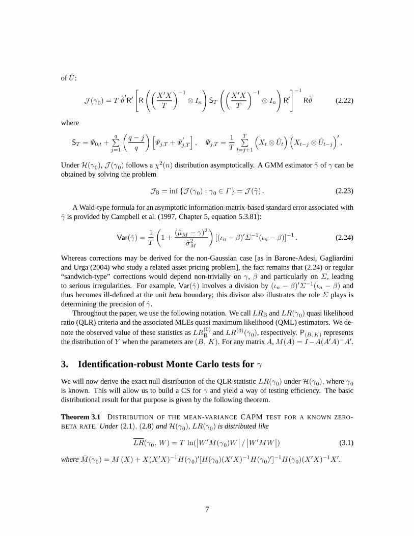
of U :

J (γ0) = T ϑ′R′

[R

((X ′X

T

)−1

⊗ In

)ST

((X ′X

T

)−1

⊗ In

)R′

]−1

Rϑ (2.22)

where

ST = Ψ0,t +q∑

j=1

(q − j

q

)[Ψj,T + Ψ

′

j,T

], Ψj,T =

1

T

T∑t=j+1

(Xt ⊗ Ut

)(Xt−j ⊗ Ut−j

)′.

UnderH(γ0), J (γ0) follows aχ2(n) distribution asymptotically. A GMM estimatorγ of γ can beobtained by solving the problem

JB = inf J (γ0) : γ0 ∈ Γ = J (γ) . (2.23)

A Wald-type formula for an asymptotic information-matrix-based standard error associated withγ is provided by Campbell et al. (1997, Chapter 5, equation 5.3.81):

Var(γ) =1

T

(1 +

(µM − γ)2

σ2M

)[(ιn − β)′Σ−1(ιn − β)]−1 . (2.24)

Whereas corrections may be derived for the non-Gaussian case [as in Barone-Adesi, Gagliardiniand Urga (2004) who study a related asset pricing problem], the fact remains that (2.24) or regular“sandwich-type” corrections would depend non-trivially on γ, β and particularly onΣ, leadingto serious irregularities. For example,Var(γ) involves a division by(ιn − β)′Σ−1(ιn − β) andthus becomes ill-defined at the unitbetaboundary; this divisor also illustrates the roleΣ plays isdetermining the precision ofγ.

Throughout the paper, we use the following notation. We callLRB andLR(γ0) quasi likelihoodratio (QLR) criteria and the associated MLEs quasi maximum likelihood (QML) estimators. We de-note the observed value of these statistics asLR

(0)B andLR(0)(γ0), respectively.P(B,K) represents

the distribution ofY when the parameters are(B, K). For any matrixA,M(A) = I−A(A′A)−A′.

3. Identification-robust Monte Carlo tests for γ

We will now derive the exact null distribution of the QLR statistic LR(γ0) underH(γ0), whereγ0is known. This will allow us to build a CS forγ and yield a way of testing efficiency. The basicdistributional result for that purpose is given by the following theorem.

Theorem 3.1 DISTRIBUTION OF THE MEAN-VARIANCE CAPM TEST FOR A KNOWN ZERO-BETA RATE. Under(2.1), (2.8) andH(γ0), LR(γ0) is distributed like

LR(γ0, W ) = T ln(∣∣W ′M(γ0)W

∣∣ /∣∣W ′MW

∣∣) (3.1)

whereM(γ0) =M (X) +X(X ′X)−1H(γ0)′[H(γ0)(X

′X)−1H(γ0)′]−1H(γ0)(X

′X)−1X ′.

7

Proofs are given in the Appendix. In thei.i.d. Gaussian case (2.9), we have:

[(T − 1− n)/n][Λ(γ0)− 1] ∼ F (n, T − 1− n) ; (3.2)

see Dufour and Khalaf (2002). This result was used by Gibbonset al. (1989) in studying efficiencywith an observable risk-free rate. Indeed, testingH(γ0) is equivalent to testing whether the inter-cepts are jointly zero in a market model with returns in excess ofγ0.

For non-Gaussian distributions compatible with (2.8) [including the GARCH case (2.12)], The-orem3.1shows that the exact distribution ofLR(γ0), although non-standard, may easily be simu-lated onceX, the distribution ofW andγ0 [given byH(γ0)] are set. So the Monte Carlo (MC) testmethod can be easily applied; see Dufour (2006). In general,this method assesses the rank of theobserved value of a test statistic

[denotedS(0)

], relative to a finite numberN of simulated statistics

[denotedS(1) , . . . , S(N)] drawn under the null hypothesis. Conforming with (2.8), weassume thatS(1) , . . . , S(N) can be simulated given: (i) a value ofν, (ii) N drawsW (1), . . . , W (N) from thedistribution ofW [which under (2.8) can be simulated onceν is specified], (iii) a vector of parame-ters (denotedη) which affects the distribution of the test statistic, and (iv) the test functionS(η, W )which depends onη, W andX.8 In other words, on drawingN samples from the distribution ofW(which may depend onν) and computingS(η, W ) for each simulated sample, we get the vectorSN (η, ν) =

[S(η, W (1)

), . . . , S

(η, W (N)

)]′. In the case ofLR(γ0), S

(0) ≡ LR(0)(γ0), η ≡

γ0, and using (3.1),S(η, W (i)

)= LR

(γ0, W

(i)). Given the above, aMC p-value is defined as:

pN [S(0)∣∣SN (η, ν)] =

NGN

[S(0) ; SN (η, ν)

]+ 1

N + 1, (3.3)

GN

[S(0) ; SN (η, ν)

]=

1

N

N∑j=1

I[0,∞)

[S(W (j), η)− S(0)

], (3.4)

whereIA[x] = 1, if x ∈ A , andIA[x] = 0, if x /∈ A . If the distribution of the statistic underconsideration, givenX, is completely determined byX and the distribution ofW givenX (whichdepends onν andη), then comparingpN [S(0)

∣∣SN (η, ν)] to anα cut-off whereα(N + 1) is aninteger yields a test with the statedsizeα: the probability of rejection under the null hypothesis isexactlyα, for finiteT andN .

If ν or η is not set by the null hypothesis, then the MMC method does allow one to control thelevel of the test: we maximizepN [S(0)

∣∣SN (η, ν)] over all the(ν, η) values compatible with the nullhypothesis, and reject the latter if the maximalp-value is less than or equal toα. Then the probabil-ity of rejection under the null hypothesis is itself not larger thanα, for finite T andN ; see Dufour(2006). In the case ofLR(γ0) with LRN (γ0, ν) =

[LR(γ0, W

(1)), . . . , LR

(γ0, W

(N))]′

, wehave:

pN (γ0, ν) ≡ pN[LR(0)(γ0)

∣∣LRN (γ0, ν)]. (3.5)

As a result of Theorem3.1, we have, underH(γ0) in conjunction withHW (D, ν) :

P[pN (γ0, ν0) ≤ α

]= α , whenν = ν0, (3.6)

P[suppN (γ0, ν) : ν ∈ ΩD ≤ α

]≤ α , whenν may be unknown. (3.7)

8For notational simplicity, the dependence uponX is implicit through the definition ofS.

8

We will call pN (γ0, ν) apivotal MC (PMC)p-value.

4. Identification-robust confidence sets forγ

UnderHB, the ratiosai/(1 − βi) , 1, . . . , n, are equal. This definition ofγ leads to the classicalproblem of inference on ratios from Fieller (1954). The problem here is clearly more complex, soto extend Fieller’s arguments, we use the above defined testsof H(γ0).

4.1. Fieller-type confidence sets: thei.i.d. Gaussian case

Consider the Gaussian model given by (2.1), (2.8) and (2.9).In this case, underH0(γ0), W(γ0)follows a Fisher distributionF (n, T − n− 1) ; see (3.2). LetFα denote the cut-off point for a testwith levelα based on theF (n, T − n− 1) distribution. Then

CFγ(α) = γ0 ∈ Γ : W(γ0) ≤ Fα (4.1)

has level1 − α for γ, i.e. the probability thatγ be covered byCFγ(α) is not smaller than1 − α :Indeed,P[γ ∈ CFγ(α)] = 1− α. On noting thatW(γ0) ≤ Fα can be rewritten as

MF (γ0)−nFα

T − n− 1NF (γ0) ≤ 0 , (4.2)

MF (γ0) =(a+ δγ0

)′Σ−1

(a+ δγ0

)=(δ′Σ−1δ

)γ20 +

(2δ

′Σ−1a

)γ0 + a′Σ−1a , (4.3)

NF (γ0) = 1 +(µM − γ0)

2

σ2M=

1

σ2Mγ20 −

2µmσ2M

γ0 + 1 +µ2Mσ2M

, (4.4)

we see, after a few manipulations, thatCFγ(α) reduces to a simple quadratic inequation:

CFγ(α) = γ0 ∈ Γ : Aγ20 +Bγ0 + C ≤ 0 , (4.5)

A = δ′Σ−1δ −

(nFα

T − n− 1

)1

σ2M, B = 2

[δ′Σ−1a+

(nFα

T − n− 1

)µMσ2M

], (4.6)

C = a′Σ−1a−

(nFα

T − n− 1

)[1 +

µ2Mσ2M

]. (4.7)

ForΓ = R, the resulting CS can take several forms depending on the roots of the polynomialAγ20 + Bγ0 + C : (a) a closed interval; (b) the union of two unbounded intervals; (c) the entirereal line; (d) an empty set.9 Case (a) corresponds to a situation whereγ is well identified, while(b) and (c) correspond to unbounded CSs and indicate (partial or complete) non-identification. Thepossibility of getting an empty CS may appear surprising. But, on hindsight, this is quite natural:it means that no value ofγ0 does allowH(γ0) to be acceptable. SinceHB states that there existsa real scalarγ such thatai = (1 − βi)γ , i = 1, . . . , n, this can be interpreted as a rejection ofHB. Further, underHB, the probability thatCFγ(α) covers the true valueγ is 1−α, and an emptyset obviously does not coverγ. Consequently, the probability thatCFγ(α) be empty[CFγ(α) = ∅]

9For further discussion, see Dufour and Jasiak (2001), Zivotet al. (1998), Dufour and Taamouti (2005), Kleibergen(2009), and Mikusheva (2009).

9

cannot be greater thanα underHB : P[CFγ(α) = ∅] ≤ α. The eventCFγ(α) = ∅, is a test withlevelα for HB under normality.

4.2. Fieller-type confidence sets with non-Gaussian non-i.i.d. errors

The quadratic CS described above relies heavily on the fact that the same critical pointFα canbe used to test all values ofγ0. This occurs under thei.i.d. Gaussian distributional assumption,but not necessarily otherwise. Although the quadratic CS will remain “asymptotically valid” aslong asW(γ0) converges to aχ2(n) distribution, this cannot provide an exact CS. The Fieller-type procedure can be extended to allow for possibly non-Gaussian disturbances, by inverting anα-level test based onW(γ0) [or equivalently onLR(γ0)] performed by simulation (as a MC test).Consider the MCp-valuepN (γ0, ν) function associated with this statistic, as defined in (3.5). Sincethe critical regionpN (γ0, ν) ≤ α has levelα for testingγ = γ0 whenν is known, the set ofγ0values for whichpN (γ0, ν) exceedsα, i.e.

Cγ(α; ν) =γ0 ∈ Γ : pN (γ0, ν) > α

, (4.8)

is a CS with level1 − α for γ. Similarly, whenν is not specified, the testsuppN (γ0, ν0) : ν0 ∈ΩD ≤ α yields:

Cγ(α; D) =γ0 ∈ Γ : suppN (γ0, ν0) : ν0 ∈ ΩD > α

, (4.9)

whose level is also1 − α. Cγ(α; ν) or Cγ(α; D) must be drawn by numerical methods. Ourempirical analysis reported below, relies on nested grid searches, overγ0 andκ, for the Student-tcase (2.10), and overγ0 and (π, ω) for the normal-mixture case (2.11); for the GARCH case (2.12),we conduct a grid search onγ0 where for each candidate value, we run the simulated annealingoptimization algorithm to calculate the maximalp-value from (4.9) over the2n nuisance parametersin φ.

We have no closed-form description of the structure ofCγ(α; ν) orCγ(α; D). While these canbe bounded intervals (this is showed numerically in Section8), Cγ(α; ν) or Cγ(α; D) must beunbounded with a high probability ifγ is not identifiable or weakly identified [see Dufour (1997)].An empty CS is also possible and provides evidence thatHB is not compatible with the data. TheeventCγ(α; ν) = ∅ [or Cγ(α; D) = ∅] is a test with levelα for HB under (2.8). The identityLR(γ) = inf LR(γ0) : γ0 ∈ Γ entails thatγ must belong to the CS, provided its level is>0.

The Hotelling-based CS we obtain for the GARCH case is exact,because the cut-off point weuse when invertingW(γ0) is adjusted for the parametric form (2.12) via the maximizedp-valuefrom (4.9). InvertingJ (γ0) in (2.22) may however be more appropriate. Again, this must beimplemented by numerical methods; for example, a grid search can be conducted onγ0 wherefor each candidate value,J (γ0) is referred to theχ2(n) distribution; this would circumvent theidentification problem asymptotically [as arguede.g. in Stock and Wright (2000)], yet in finitesamples, theχ2(n) approximation may perform poorly. Indeed, our simulation results reportedbelow illustrate the severity of this problem. Consequently, we use the MMC method for eachcandidateγ0: we maximize over the model parameters as well as overφ.10

10We have observed a numerical invariance toB andK, which calls for further theoretical work with such statistics;see also Section 7.

10

5. Invariance and exact distribution ofLRB

In this section, we study the exact distribution of the statisticsLR(γ0) andLRB, under both the nullhypothesis and the corresponding unrestricted MLR alternative model. We track and control for thejoint role betasand scale parameters play in identifyingγ.

Lemma 5.1 MULTIVARIATE SCALE INVARIANCE . The LR statisticsLR(γ0) andLRB defined in(2.18) and(2.14) are invariant to replacingY by Y∗ = Y A, whereA is an arbitrary nonsingularn× n matrix.

Such transformations can be viewed as the following affine transformations onY :

Y∗ = Y A+ RM ι′n(In −A). (5.1)

Theorem 5.2 EXACT DISTRIBUTION OF BCAPM LR TESTS. Under(2.1) and(2.8), the distri-butions ofLR(γ0) andLRB depend on(B,K) only throughB = (B −∆)K−1, and

LR(γ0) = T ln(|W (γ0)

′W (γ0)|/|W′W |

), LRB = inf LR(γ0) : γ0 ∈ Γ , (5.2)

where∆ = [0, ιn]′, W =M(X)W , M(γ0) is defined as in(3.1) and

W (γ0) = M(γ0)(XB +W ) = M(γ0)ιT [a+ γ0(β − ιn)]′K−1 +W . (5.3)

If, furthermore, the null hypothesisHB holds, then

W (γ0) = (γ0 − γ)M(γ0)ιT (β − ιn)′K−1 + M(γ0)W (5.4)

and the distribution ofLRB depends on(B,K) only throughγ and(β− ιn)′K−1; in the Gaussian

case(2.9), this distribution involves only one nuisance parameter.

Even thoughB andK may involve up to2n+ n2 different nuisance parameters [or2n+n(n+1)/2 parameters, ifK is triangular], the latter theorem shows that the number of free parametersin the distributions ofLR(γ0) andLRB does not exceed2n; whenHB holds, the number of freeparameters is at mostn+ 1. Further, underH(γ0) [using (5.4)]B is evacuated, entailing Theorem3.1. Theorem5.2also provides the power function.

6. Exact bound procedures for testingHB

In this section, we propose tests forHB in the presence of nuisance parameters induced by nonlin-earity and non-Gaussian error distributions. We study firstglobal bounds based on tests ofH(γ0)where we outline important differences between the Gaussian and non-Gaussian cases. Second,we describe more general but computationally more expensive methods based on the technique ofMMC tests to obtain tighter bounds.

6.1. Global bound induced by tests ofH(γ0)

The results of Section 3 on testingγ = γ0 can be used to derive a global bound on the distributionof the statisticLRB. This is done in the following theorem.

11

Theorem 6.1 GLOBAL BOUND ON THE NULL DISTRIBUTION OF THE BCAPM TEST. Under theassumptions(2.1), (2.8) andHB, we have, for any givenν ∈ ΩD,

P[LRB ≥ x

]≤ sup

γ0∈ΓP[LR(γ0, W ) ≥ x

], ∀x , (6.1)

whereLR(γ0, W ) is defined in(3.1). Further, in the Gaussian case(2.9), we have:

P[(T − 1− n) (ΛB − 1) /n ≥ x

]≤ P[F (n, T − 1− n) ≥ x] , ∀x . (6.2)

To relate this result to available bounds, observe that (6.1) and (6.2) easily extend to the follow-ing multi-beta setups: fori = 1, . . . , n, t = 1, . . . , T,

Rit = ai +s∑

j=1βijRjt + uit , HB : ai = γ

(1−

s∑j=1

βij

), (6.3)

whereRjt, j = 1, ... , s, are returns ons benchmarks. In this case, the bounding distributionof LRB obtains as in Theorem6.1 whereX = [ιT , R1, ... , Rs] , Rj = (Rj1, ... , RjT )

′,j = 1, . . . , s, andH is the k-dimensional row vector(1, γ0, . . . , γ0). In the Gaussian case,P[LR(γ0, W ) ≥ x

]does not depend onγ0, and the bounding distribution under normality is

F (n, T − s− n). Shanken (1986) suggested the statistic

Q = minγ

T[a− γ(ιn − βιs)

]′[(T/(T − 2)

)Σ]−1[

a− γ(ιn − βιs)]

1 + (RM − γιs)′∆−1M (RM − γιs)

(6.4)

where a is ann-dimensional vector which includes the (unconstrained) intercept estimates,β isan n × s matrix whose rows include the unconstrained OLS estimates of (βi1, . . . , βis), i =1, . . . , n, RM and∆M include respectively the time-series means and sample covariance matrixcorresponding to the right-hand-side total portfolio returns. Further, the minimum in (6.4) occurs atthe constrained MLEγ of γ, and

LRB = T ln(1 + Q/(T − s− 1)). (6.5)

For normal errors,(T−s−n)Q/[n(T −s−1)] can be bounded by theF (n, T −n−s)distribution.The latter obtains from Gibbons et al.’s (1989) joint test ofzero intercepts, where returns are ex-pressed in excess of a knownγ.

Independently, Stewart (1997) showed [using Dufour (1989)] that, under normal errors,(T −s− n)

[(|ΣB|/|Σ|

)− 1]/n can be bounded by theF (n, T − n− s)distribution. Now, from (2.18)

and (6.5), we see that Shanken and Stewart’s bounds are equivalent, and both results obtain fromTheorem6.1 in the special case of normal errors.

When disturbances are non-Gaussian, Theorem6.1 entails that the bounding distribution caneasily be simulated, as follows. Given a value ofν, generateN i.i.d. draws from the distributionof W1, . . . , WT ; then, for any givenγ0, these yield a vectorLRN (γ0, ν) of N simulated valuesof the test statisticLR(γ0, W ), as defined in (3.1). A MCp-value may then be computed from therank of the observed statisticLRB relative to the simulated values. Denote this MCp-value by

pUN (γ0, ν) ≡ pN [LR(0)B

∣∣LRN (γ0, ν)] (6.6)

12

whereLR(0)B represents the value of the test statisticLRB based on the observed data; we will

call pUN (γ0, ν) thebound MC(BMC) p-value. In contrast with the Gaussian case,pUN [γ0, ν] maydepend onγ0; nevertheless, for anyγ0,

LRB ≤ LR(γ0) ⇒ pN (γ0, ν) ≤ pUN (γ0, ν). (6.7)

So a critical region that provably satisfies the level constraint can be obtained by maximizingpUN (γ0, ν) over the relevant nuisance parameters. To simplify presentation of this result, we in-troduce the following notation. For any subsetsA ⊆ Γ andE ⊆ ΩD, let

pUN (γ0, E) = sup pUN (γ0, ν0) : ν0 ∈ E, pUN (A, ν0) = sup pUN (γ0, ν0) : γ0 ∈ A, (6.8)

pUN (A, E) = sup pUN (γ0, ν0) : γ0 ∈ A, ν0 ∈ E, (6.9)

where, by convention,pUN (A, · ) = 0 if A is empty, andpUN ( · , E) = 0 if E is empty.

Theorem 6.2 GLOBAL SIMULATION -BASED BOUND ON THE NULL DISTRIBUTION OF THE

BCAPM TEST STATISTIC. Under(2.1), (2.8) andHB, we have:

P[pUN (Γ, ν) ≤ α

]≤ α , P

[pUN (Γ, ΩD) ≤ α

]≤ α , (6.10)

whereν represents the true distributional shape ofW .

The first inequality in (6.10) holds for a statistic that requires the value ofν, while the secondone holds even without the need to specifyν. These bound tests are closely related to the CS-based test proposed in Section 4: the null hypothesis is rejected when the CS forγ is empty,i.e.if no value ofγ0 can be deemed acceptable (at levelα), either withν specified orν taken as anuisance parameter. This may be seen on comparing (4.9) withthe probabilities in Theorem6.2.On recalling thatLRB = inf LR(γ0) : γ0 ∈ Γ , the latter also suggests a relatively easy way ofshowing thatCγ(α; ν) or Cγ(α; D) is not empty, through the specificp-value pUN (γ, ν) obtainedby takingγ0 = γ in (6.6). We shall callpUN (γ, ν) theQML-BMCp-value.

Theorem 6.3 RELATION BETWEEN EFFICIENCY TESTS AND ZERO-BETA CONFIDENCE SETS.Under(2.1), (2.8) andHB, let γ be the QML estimator ofγ in (2.19). Then,

pUN (γ, ν) > α⇒ sup pN (γ0, ν) : γ0 ∈ Γ > α⇒ Cγ(α; ν) 6= ∅ , ∀ν ∈ ΩD ,

pUN (γ, ΩD) > α⇒ suppN (γ0, ν0) : γ0 ∈ Γ, ν0 ∈ ΩD > α⇒ Cγ(α; D) 6= ∅ ,

whereCγ(α, ν) andCγ(α; D) are the sets defined in(4.8) and(4.9).

For the Gaussian case, Zhou (1991) and Velu and Zhou (1999) proposed a potentially tighterbound applicable to statistics which can be written as ratios of independent Wishart variables anddoes not seem to extend easily to other classes of distributions. In the next section, we propose anapproach which yields similarly tighter bounds for non-Gaussian distributions as well. Finally, theHAC statisticJB may be used to obtain alternative identification-robust bound tests following thesame rationale. The correspondence between such tests and empty CSs entailed by test inversionalso follows from similar arguments. Finite-sample MMC level corrections are recommended, giventhe simulation results in Section 7.

13

6.2. Maximized Monte Carlo bounds

Another approach to testingHB with the statisticLRB consists in directly assessing its depen-dence on nuisance parameters and adjusting the test accordingly through the MMC method [Dufour(2006)]. Letθ = ψ(B, K) represent the parameter vector upon which the distributionof LRB

actually depends, andΩB the set of admissible values forθ underHB. The dimension ofθ may belower than than the number of parameters inB andK. To conform with our earlier notation for MCp-values, we define the functionLRB(θ, W ) = LRB

(ψ(B, K), W

)which assigns to each value

of (B, K) and the noise matrixW the following outcome: usingθ and a draw from the distributionof W (which may depend onν), generate a sample from (2.1)-(2.2), and computeLRB [as definedin (2.18)] from this sample.

On applyingLRB(θ, W ), we can get simulated values from the null distribution ofLRB forany value ofθ. If N independent replicationsW (1), . . . , W (N) of W are generated, we canthen compute the corresponding vector ofLRB statistics and thep-value functionpBN (θ, ν) =

pN[LR

(0)B

∣∣LRBN (θ, ν)],whereLRBN (θ, ν) =

[LRB

(θ, W (1)

), . . . , LRB

(θ, W (N)

)]′. For

any given value ofν, the MMCp-value associated withLR(0)B is obtained by maximizingpBN (θ, ν)

with respect toθ over the set of admissible valuesΩB underHB :

pMBN (ΩB, ν) = sup pBN (θ, ν) : θ ∈ ΩB . (6.11)

Then, underHB and the error distribution associated withν, we have:P[pMBN (ΩB, ν) ≤ α

]≤ α ;

see Dufour (2006). In other words,pMBN (ΩB, ν) ≤ α is a critical region with levelα. Further,in order to allow for an unknownν, we can maximizepBN (θ, ν) with respect toν ∈ ΓD. Set:pMBN (θ, ΩD) = sup pBN (θ, ν) : ν ∈ ΩD , p

MBN (ΩB, ΩD) = sup pMBN (θ, ΩD) : θ ∈ ΩB .

Then, underHB, P[pMBN (ΩB, ΩD) ≤ α

]≤ α .

Theorem6.3 guarantees thatpUN (Γ, ν) ≤ α ⇒ pMBN (ΩB, ν) ≤ α for any givenν. So it maybe useful to check the global bound for significance before turning to the MMC one. Furthermore,it is not always necessary to run the numerical maximizationunderlying MMC to convergence: ifpBN (θ, ν) > α given any relevantθ (or ν), then a non-rejection is confirmed. We suggest to usethe QML estimateθ of θ as start-up value, because this providesparametric bootstrap-type[or alocal MC (LMC)] p-values:

pbN (ν) = pBN(θ, ν) , pbN (ΩD) = pBN (θ, ΩD) . (6.12)

ThenpbN (ν) > α entailspMBN (ΩB, ν) > α, andpbN (ΩD) > α entailspMBN (ΩB, ΩD) > α.Finally, a parametric MMC test imposing (2.12) may be applied to the HAC statisticsJ (γ0)

andJB, as an attempt to correct their size for the GARCH alternative of interest. We investigate thesize-corrected power associated with these statistics in Section 7.

6.3. Two-stage bound confidence procedures

To deal with the fact that the distribution ofW may involve an unknown parameterν ∈ ΩD,we suggested above to maximize the relevantp-values overΩD. We next consider restricting themaximization overν to a set which is empirically relevant, as in Beaulieu et al. (2007). This leads totwo basic steps: (i) an exact CS with level1−α1 is built for ν, and (ii) the MCp-values (presentedabove) are maximized over all values ofν in the latter CS and are referred to the levelα2, so that

14

the global test level isα = α1 + α2. In our empirical application, we usedα/2. Let Cν(α1) =Cν(α1; Y ) be a CS with level1 − α1 for ν. Then, underH(γ0), we haveP

[pUN [γ0, Cν(α1)] ≤

α2

]≤ α1 + α2 while, underHB :

P[pUN [Γ, Cν(α1)] ≤ α2

]≤ α1 + α2 , P

[pMBN [ΩB, Cν(α1)] ≤ α2

]≤ α1 + α2 . (6.13)

Note also that forpMBN [ΩB, Cν(α1)] ≤ α2 not to hold, the following condition is sufficient:

pMBN (θ, Cν(α1)) > α2. (6.14)

To build a CSs forν, we invert a test (of levelα1) for the specification underlying (2.8) whereν = ν0 for knownν0; this avoids the need to use regularity assumptions onν. The test we invert isthe three-stage MC GF test introduced in Dufour et al. (2003):

CSK = 1−min p [ESK(ν0)] , p [EKU(ν0)] (6.15)

whereESK(ν0) =∣∣SK−SK(ν0)

∣∣, SK = 1T 2

∑Tt=1

∑Ti=1 d

3it, EKU(ν0) =

∣∣KU−KU(ν0)∣∣,

KU = 1T

∑Tt=1 d

2tt, dit are the elements of the matrixU(U ′U/T )−1U ′, SK(ν0) and KU(ν0)

are simulation-based estimates of the expectedSK and KU given (2.8) andp [ESK(ν0)] andp [EKU(ν0)] arep-values, obtained by MC methods under (2.8). The MC test technique is alsoapplied to obtain a size correctp-value forCSK. The CS forν corresponds to the values ofν0which are not rejected at levelα1, using the latterp-value.

To conclude, we note that for the GARCH case, pre-estimatingthe2n× 1 vectorφ is infeasiblewith 5 or even 10 year sub-samples of monthly data. Nevertheless, the single stage MMC is validdespite this limitation. Interestingly, the simulation study we report next suggests that power costsare unimportant even with relatively small samples.

7. Simulation study

We now present a small simulation study to assess the performance of the proposed methods.The design is calibrated to match our empirical analysis (see Section 8) which relies on monthlyreturns of 12 portfolios of NYSE firms over 1927-1995. We consider model (2.1) whereRMt,t = 1, . . . , T , are the returns on the market portfolio from the aforementioned data over the last5 and 10 year subperiods, as well as the whole sample. We thus taken = 12 andT = 60, 120and828. The coefficients of (2.1) includingγ are set to their QML estimates (restricted underHB

over the conformable sample period). From the QML regression, we also retain the estimated errorcovariance matrix, to generate model shocks; formally, we compute the corresponding empiricalCholesky factor (denotedK) and use it forK in (2.8). Test sizes withK = I12 are also analyzed toillustrate the effects of portfolio repacking.

We consider normal and Studentt-errors (withκ = 8, in accordance with the kurtosis observedin the empirical application), so the random vectorsWt, t = 1, . . . , T , in (2.8) are generatedfollowing (2.9) and (2.10) respectively. The MC tests are applied imposing and ignoring informationon κ, which allows us to document the cost of estimating this parameter. Whenκ is consideredunknown, MMCp-values are calculated over the interval4 ≤ κ ≤ 13 to keep execution timemanageable (a wider range is allowed for the empirical application in Section 8). We also consider

15

the case of GARCH errors (2.12), withφ1i = φ1 andφ2i = φ2, i = 1, . . . , n (the coefficientsare the same across equations). This restriction is motivated by execution time, but it is relaxed inSection 8. We use the diagonal elements ofKK ′ to scale the intercept, yet we also consider the casewhereσ2i = 1, i = 1, . . . , n. Samples are simulated with(φ1, φ2) = (.15, .80). These parametersare treated, in turn, as known and as unknown quantities. In view of the low dimension of thenuisance parameter space in this case, when(φ1, φ2) is treated as unknown,p-value maximizationis achieved through a coarse grid search (for the purpose of this simulation). Thep-value functiondoes not appear to be very sensitive to the value of(φ1, φ2), and the results presented below indicatethis is sufficient for controlling test level in the relevantcases. A more thorough optimization ishowever used in Section 8.

The results of the simulation are summarized in Tables 1 - 3. These tables report empiricalrejection rates for various tests ofH(γ0) with nominal size5%. These rejection rates determinethe coverage properties of confidence sets derived from the tests. Since we focus on estimatingγ, HB is imposed for both the size and power studies. We compare thefollowing tests: (1) aWald-type test which rejectsγ = γ0 whenγ0 falls outside the Wald-type confidence interval[γ −1.96×AsySE(γ), γ+1.96× AsySE(γ)], using the QML estimatorγ, an asymptotic standard error[AsySE(γ), based on (2.24)], and a normal limiting distribution; (2) the MC and MMC tests basedon the QLR test statisticLR(γ0) defined in Theorem3.1, with MC p-values fori.i.d. normal orStudent-t errors (with known or unknownκ), Gaussian GARCH with known or unknown(φ1, φ2),as well as asφ1 = φ2 = 0 (i.e., ignoring the GARCH dependence even when it is present in thesimulated process); (3) tests based on the HAC Wald-type statistic J (γ0) in (2.22), using aχ2(n)critical value, MC with known(φ1, φ2), and MMC where(φ1, φ2) is taken as unknown.

In the size study (Table 1),γ0 is calibrated to its QML counterpart from the data set [γ0 =−0.000089 for T = 60, γ0 = .004960 for T = 120, γ0 = .005957 for T = 828]. In the powerstudy (tables 2 - 3), we focus on theK case; samples are drawn withγ set to its QML estimate, andγ0 is set to the latter value +step ×σmin

i , whereσmini = [minσ2i ]

1/2, andσ2i are the diagonalterms ofKK ′ (with variousstep values).N = 99 is used for MC tests (N = 999 is used in theempirical application). In each experiment, the number of simulations is 1000. We use 12 lags forthe HAC correction.

Our results can be summarized as follows. The asymptotici.i.d. or robust procedures are veryunreliable from the viewpoint of controlling level. Whereas we observe empirical frequencies oftype I errors over70% and sometimes90% with T = 60, we still see empirical rejections near55% with T = 828. The results also show that the empirical size of the HAC-based tests is notaffected byK, though a formal proof of its invariance is not available. This observation is howevercompatible with the fact that its size improves with larger samples: while the level of the Wald-typetest shows no improvement (around55%) even withT = 828 and normal errors, the size of theWald-HAC statistic drops from95% with T = 60 to 12% with T = 828. The LR and robust MCand MMC tests achieve level control; in the GARCH case, the MCLR test has the correct size evenwhen GARCH dependence is not accounted for.

In view of the poor size performance of the asymptotic tests,the power study focuses on pro-cedures whose level appears to be under control. Overall, the MMC correction is not too costlyfrom the power viewpoint, with both Student-t and GARCH errors. In the latter case, the LR-typetest uncorrected for GARCH effects outperforms all the other tests. When GARCH corrections areperformed via MMC, the LR-type test performs generally better than the Wald-HAC test.

16

Table 1. Tests on zero-beta rate: empirical size

n = 12 T = 60, T = 120 T = 828

K K K

Test I12 K I12 K I12 K

i.i.d. NormalWald-type .709 .196 .633 .096 .578 .050LR(γ0), MC .057 .057 .048 .048 .041 .041

i.i.d. Student-tWald-type .714 .218 .645 .106 .587 .055

LR(γ0), MC, κ known .053 .053 .046 .046 .043 .043LR(γ0), MMC, κ unknown .043 .043 .035 .035 .031 .031

Gaussian GARCHWald-type .676 .200 .628 .086 .579 .047

LR(γ0), MC, φ1 = φ2 = 0 .059 .059 .048 .048 .046 .046J (γ0), χ

2(12) .954 .954 .686 .686 .127 .127J(γ0), MMC, φ1, φ2 known .049 .049 .045 .045 .049 .040J(γ0), MMC, φ1, φ2 unknown .040 .040 .034 .034 .040 .049LR(γ0), MC, φ1, φ2 known .064 .064 .043 .043 .050 .028

LR(γ0), MMC, φ1, φ2 unknown .054 .054 .032 .032 .028 .050

–

Note – The table reports the empirical rejection rates of various tests forH(γ0) with nominal level5%. The values of

γ0

tested are:γ0= −0.000089 for T = 60, γ

0= .004960 for T = 120, γ

0= .005957 for T = 828. The design

is calibrated to match our empirical analysis (see Section 8). The tests compared are the following. (1) A Wald-type

test which rejectsγ = γ0

whenγ0

falls outside the Wald-type confidence interval[γ − 1.96 × AsySE(γ), γ + 1.96 ×

AsySE(γ)], using the QML estimatorγ with asymptotic standard error[AsySE(γ)] based on (2.24), and a normal

limiting distribution. (2) MC and MMC tests based onLR(γ0) in (2.14), with MCp-values fori.i.d. normal and Student-

t errors (with known or unknownκ), Gaussian GARCH with known or unknown(φ1, φ

2), as well asφ

1= φ

2= 0 (i.e.,

ignoring the GARCH dependence even when it is present in the simulated process). (3) Tests based on the HAC Wald-

type statisticJ (γ0) in (2.22), using aχ2(n) critical value, MC with known(φ

1, φ

2), and MMC where(φ

1, φ

2) is taken

as unknown. In thei.i.d. cases, the errors are generated using (2.8) withK set to eitherI12 or K, which corresponds to

the Cholesky factor of the least-squares error covariance estimate from the empirical data used for the simulation design.

In the GARCH case, samples are generated with conditional variance as in (2.12) usingK or I12 for K.

17

Table 2. Tests on zero-beta rate: empirical powerGaussian and Student designs

-

n = 12 T = 60 T = 120 T = 828

Test Step Power Step Power Step Poweri.i.d. normal

LR(γ0), MC, φ1 = φ2 = 0 .50 .151 .50 .226 .20 .129.75 .315 .75 .529 .30 .3131.0 .544 1.0 .835 .50 .8142.0 .981 1.5 .999 .75 .998

i.i.d. Student-tLR(γ0), MC, κ known .50 .134 .50 .181 .20 .109

LR(γ0), MMC, κ unknown .126 .158 .080LR(γ0), MC, κ known .75 .264 .75 .428 .30 .237

LR(γ0), MMC, κ unknown .239 .384 .182LR(γ0), MC, κ known 1.0 .494 1.0 .709 .50 .660

LR(γ0), MMC, κ unknown .440 .673 .605LR(γ0), MC, κ known 2.0 .939 1.5 .997 .75 .966

LR(γ0), MMC, κ unknown .925 .997 .960

Note – The table reports the empirical rejection rates of various tests forH(γ0) with nominal level5%. The values of

γ0

tested are:γ0= −0.000089 for T = 60, γ

0= .004960 for T = 120, γ

0= .005957 for T = 828. The sampling

design conforms with the size study, for theK case. Samples are drawn withγ calibrated to its QML counterpart from

the 1991-95 subsample; values forγ0

are set to the latter value +step ×σmin

i , whereσmin

i = [minσ2

i ]1/2, andσ2

i are

the diagonal terms ofKK′. See Table 1 for further details on the design and tests applied.

8. Empirical analysis

In this section, we assessHB as defined in (2.2) in the context of (2.1) under the distributionalassumptions (2.10)-(2.11), as well as the Gaussian GARCH in(2.12). We use real monthly returnsover the period going from January 1926 to December 1995, obtained from CRSP. The data studiedinvolve 12 portfolios of NYSE firms grouped by standard two-digit industrial classification (SIC).The sectors studied include: (1) petroleum; (2) finance and real estate; (3) consumer durables; (4)basic industries; (5) food and tobacco; (6) construction; (7) capital goods; (8) transportation; (9)utilities; (10) textile and trade; (11) services; (12) leisure; for details on the SIC codes, see Beaulieuet al. (2007). For each month, the industry portfolios include the firms for which the return, theprice per common share and the number of shares outstanding are recorded by CRSP. Furthermore,portfolios are value-weighted in each month. We measure themarket return by value-weightedNYSE returns, and the real risk-free rate by the one month Treasury bill rate net of inflation, bothavailable from CRSP. All MC tests were applied withN = 999 and MMCp-values are obtainedusing the simulated annealing algorithm.

Our QML-based BCAPM test results are summarized in Table 4. Non-Gaussianp-values are thelargest MCp-values over the error distribution parameters [respectively: κ and(π, ω) for (2.10)-(2.11)] within the specified 97.5% CSs; the latter are reported in Table 5. In the GARCH case (2.12),p-values are the largest MCp-values over all (φ1i, φ2i). Given a5% level test, the benchmark is

18

Table 3. Tests on zero-beta rate: empirical powerGaussian GARCH design

n = 12 T = 60 T = 120 T = 828

Test Step Power Step Power Step PowerLR(γ0), MC, φ1 = φ2 = 0 .50 .112 .50 .203 .20 .195J (γ0), MMC, φ1, φ2 known .088 .155 .208J(γ0), MMC, φ1, φ2 unknown .078 .133 .183LR(γ0), MC, φ1, φ2 known .113 .204 .198

LR(γ0), MMC, φ1, φ2 unknown .106 .170 .168

LR(γ0), MC, φ1 = φ2 = 0 .75 .247 .75 .449 .30 .465J(γ0), MMC, φ1, φ2 known .177 .316 .442J(γ0), MMC, φ1, φ2 unknown .158 .276 .411LR(γ0), MC, φ1, φ2 known .248 .452 .471

LR(γ0), MMC, φ1, φ2 unknown .213 .411 .425

LR(γ0), MC, φ1 = φ2 = 0 1.0 .447 1.0 .753 .50 .945J(γ0), MC, φ1, φ2 known .300 .552 .934

J(γ0), MMC, φ1, φ2 unknown .269 .505 .920LR(γ0), MC, φ1, φ2 known .441 .753 .950

LR(γ0), MMC, φ1, φ2 unknown .395 .709 .937

LR(γ0), MC, φ1 = φ2 = 0 2.0 .913 1.5 .973 .75 1.0J(γ0), MMC, φ1, φ2 known .719 .856 1.0J(γ0), MMC, φ1, φ2 unknown .664 .931 1.0LR(γ0), MC, φ1, φ2 known .915 .970 1.0

LR(γ0), MMC, φ1, φ2 unknown .892 .962 1.0

Note – The values ofγ0

tested are:γ0= −0.000089 for T = 60, γ

0= .004960 for T = 120, γ

0= .005957 for

T = 828. Numbers reported are empirical rejection rates for various tests ofH(γ0) with nominal size5%. The sampling

design conforms with the size study, for theK case; errors are generated with conditional variance as in (2.12) usingK.

See Table 1 for a complete description of the designs and tests applied. Samples are drawn withγ calibrated to its QML

counterpart from the 1991-95 subsample; values forγ0

are set to -the latter value +step×σmin

i (for variousstep values)

whereσmin

i = [minσ2

i ]1/2, andσ2

i are the diagonal terms ofKK′.

.05 for p∞, normal LMC, MMC and GARCHp-values, while the Student-t and normal mixturep-values should be compared to.025 (to ensure that the test has level.05). Non-rejections by LMCMC p-values are conclusive (though rejections are not); rejections based on the conservative boundreported under the heading BND are conclusive under normality; non-rejections based on the QMLbound in the non-Gaussian case (reported under the heading BND) signal that the CS forγ is notempty; however, since the MMCp-value is based on the tightest bound, this evidence does notnecessarily imply non-rejection ofHB.

The empirical results presented in Table 4 show that the asymptotic test and the Gaussian-based bound test yield the same decision at level5%, although the formerp-values are much lower.The non-normalp-values exceed the Gaussian-basedp-value, enough to change the test decision.For instance, at the5% significance level, we find seven rejections of the null hypothesis for theasymptoticχ2(11) test, seven for the MCp-values under normality and with normal GARCH, and

19

Table 4. QML-based tests of BCAPM

Sample LRB p∞ Normal GARCH

LMC MMC BND BND

1927 − 30 16.10 .137 .269 .308 .366 .3401931 − 35 14.09 .228 .344 .381 .432 .4511936 − 40 15.36 .167 .257 .284 .345 .3551941 − 45 18.62 .068 .148 .163 .203 .2131946 − 50 32.69 .001 .005 .006 .007 .0061951 − 55 37.04 .000 .003 .004 .004 .0031956 − 60 26.10 .006 .027 .031 .042 .0391961 − 65 29.21 .002 .011 .016 .020 .0151966 − 70 27.45 .004 .016 .018 .026 .0291971 − 75 16.81 .113 .213 .224 .292 .2941976 − 80 25.76 .007 .027 .031 .040 .0421981 − 85 14.98 .183 .316 .335 .387 .4041986 − 90 35.41 .000 .003 .004 .004 .0051991 − 95 16.41 .127 .219 .253 .310 .320

Student-t Normal mixtureLMC MMC BND LMC MMC BND

1927 − 30 .272 .316 .360 .279 .313 .3811931 − 35 .359 .399 .468 .342 .387 .4521936 − 40 .282 .308 .372 .265 .302 .3571941 − 45 .147 .169 .210 .150 .165 .2111946 − 50 .007 .007 .010 .007 .007 .0081951 − 55 .003 .005 .005 .003 .003 .0031956 − 60 .030 .040 .052 .028 .035 .0451961 − 65 .013 .017 .023 .014 .021 .0241966 − 70 .020 .025 .032 .018 .023 .0281971 − 75 .217 .248 .300 .206 .238 .2921976 − 80 .026 .035 .039 .026 .034 .0421981 − 85 .323 .399 .405 .318 .339 .4061986 − 90 .004 .005 .005 .004 .004 .0051991 − 95 .226 .263 .325 .226 .261 .319

Note –LRB is the statistic in (2.18). Remaining numbers are associated p-values. p∞ is based onχ2(n − 1). All

other non-Gaussianp-values are the largest MCp-values over the shape parameterν within the specified CSs [ν = κ or

ν = (π, ω); refer to Table 5]. LMC is the bootstrapp-value in (6.14) and MMC is the maximalp-value in (6.13) (refer to

Section 6.2). BND is the bound (6.2) for the Gaussian case andtheQML-BMCbound from Theorem6.3otherwise; the

GARCH BND is the largestQML-BMCoverφ1i, φ2i [from (2.12)]. Returns for the months of January and for October

1987 are excluded. Given a5% level, the cut-off is .05 forp∞, the normal LMC, MMC and the GARCHp-values; for

the Student-t and mixtures, the cut-off is .025.p-values which lead to significant tests with this benchmark are in bold.

20

Table 5. Confidence sets for intervening parameters

Mixture (π, ω), confidence set forω t(κ)

(1) (2) (3) (4) (5) (6)

Sample π = 0.1 π = 0.2 π = 0.3 π = 0.4 π = 0.5 κ

1927 − 30 ≥ 1.8 1.6 − 2.8 1.6− 2.5 1.6− 2.5 1.6− 2.6 3− 121931 − 35 2.1− 10.0 1.9 − 3.0 1.9− 2.7 1.9− 2.7 2.1− 3.0 3− 81966 − 40 1.5− 3.5 1.5 − 2.3 1.4− 2.1 1.4− 2.0 1.4− 2.1 4− 251941 − 45 1.3− 3.5 1.3 − 2.1 1.3− 1.9 1.3− 1.8 1.3− 1.9 ≥ 51946 − 50 1.4− 3.5 1.3 − 2.2 1.3− 2.0 1.3− 1.9 1.3− 1.9 5− 371951 − 55 1.4− 3.5 1.4 − 2.2 1.3− 2.0 1.3− 1.9 1.3− 2.0 5− 341956 − 60 1.3− 2.8 1.2 − 2.0 1.2− 1.9 1.2− 1.8 1.2− 1.8 ≥ 51961 − 65 1.0− 2.2 1.0 − 1.6 1.0− 1.5 1.0− 1.5 1.0− 1.5 ≥ 71966 − 70 1.3− 3.0 1.3 − 2.0 1.3− 1.9 1.3− 1.8 1.2− 1.9 ≥ 51971 − 75 1.5− 3.5 1.5 − 2.2 1.4− 2.0 1.4− 1.9 1.4− 2.0 4− 241976 − 80 1.6− 4.0 1.5 − 2.5 1.5− 2.2 1.5− 2.2 1.5− 2.3 4− 191981 − 85 1.4− 3.5 1.4 − 2.1 1.3− 2.0 1.3− 1.9 1.4− 2.0 5− 331986 − 90 1.1− 3.0 1.1 − 2.0 1.1− 1.8 1.0− 1.7 1.1− 1.8 ≥ 51991 − 95 1.0− 1.9 1.0 − 1.5 1.0− 1.4 1.0− 1.3 1.0− 1.3 ≥ 19

Note – Numbers in columns (1)-(5) represent a CS for the parameters(π, ω) [respectively, the probability of mixing

and the ratio of scales] of the multivariate mixtures-of-normal error distribution. Column (6) presents the CS forκ, the

degrees-of-freedom parameter of the multivariate Student-t error distribution. See Section 6 for details on the construc-

tion of these CSs: the values of(π, ω) or κ (respectively) in this set are not rejected by theCSK test (6.15) [see Dufour

et al. (2003)] under multivariate mixtures or Student-t errors (respectively). Note that the maximum of thep-value occurs

in the closed interval forω. Returns for the month of January and October 1987 are excluded from the data set.

five (relying on the MMCp-value) under the Student-t and normal mixture distributions.Focusing on Student-t and normal mixture distributions with parameters not rejected by proper

GF tests, we see that mean-variance efficiency test results can change relative to the availableF -based bound. The power advantages of the MMC procedure are illustrated by the results of the1966-70 subperiod where the QMLp-value exceeds2.5% for the Student-t and normal mixturedistributions, whereas the MMCp-value signals a rejection.

The CSs for distributional parameters are reported in Table5. In the mixture case, the confidenceregion is summarized as follows for presentation ease: we give the CS forω corresponding to fivedifferent values ofπ.

In Table 6, we present: (i) the average real market return as well as the average real risk-freerate over each subperiod, (ii) the QML estimate ofγ (denotedγ) and95% CSs for this parameter,using respectively the asymptotic standard errors (2.24) (under the heading Wald-type), and the LR-type tests withi.i.d. Gaussian,t(κ) and normal mixture(π, ω) errors, plus Gaussian GARCH errors(lower panel).11 The values ofγ in the Fieller-type CS are not rejected by the test defined in Theorem

11Note that some values ofγ are high. Nonetheless, comparing the average real market return for those subperiodswith our estimate ofγ reveal that these high occurrences ofγ are consistent with subperiods during which the estimatedzero-beta rate is higher than the market portfolio return. This is an illustration of finding, ex post, a linear relationship

21

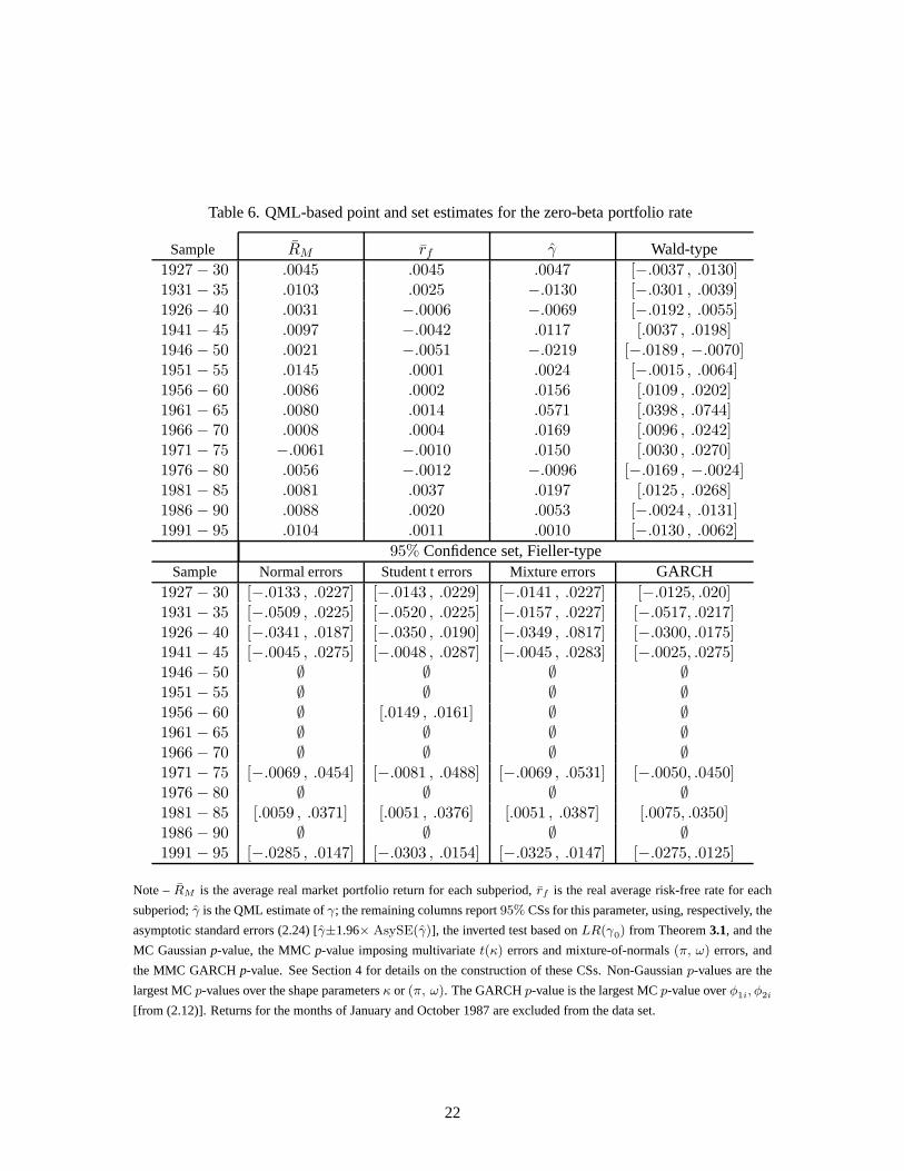
Table 6. QML-based point and set estimates for the zero-betaportfolio rate

Sample RM rf γ Wald-type1927 − 30 .0045 .0045 .0047 [−.0037 , .0130]1931 − 35 .0103 .0025 −.0130 [−.0301 , .0039]1926 − 40 .0031 −.0006 −.0069 [−.0192 , .0055]1941 − 45 .0097 −.0042 .0117 [.0037 , .0198]1946 − 50 .0021 −.0051 −.0219 [−.0189 , −.0070]1951 − 55 .0145 .0001 .0024 [−.0015 , .0064]1956 − 60 .0086 .0002 .0156 [.0109 , .0202]1961 − 65 .0080 .0014 .0571 [.0398 , .0744]1966 − 70 .0008 .0004 .0169 [.0096 , .0242]1971 − 75 −.0061 −.0010 .0150 [.0030 , .0270]1976 − 80 .0056 −.0012 −.0096 [−.0169 , −.0024]1981 − 85 .0081 .0037 .0197 [.0125 , .0268]1986 − 90 .0088 .0020 .0053 [−.0024 , .0131]1991 − 95 .0104 .0011 .0010 [−.0130 , .0062]

95% Confidence set, Fieller-typeSample Normal errors Student t errors Mixture errors GARCH

1927 − 30 [−.0133 , .0227] [−.0143 , .0229] [−.0141 , .0227] [−.0125, .020]1931 − 35 [−.0509 , .0225] [−.0520 , .0225] [−.0157 , .0227] [−.0517, .0217]1926 − 40 [−.0341 , .0187] [−.0350 , .0190] [−.0349 , .0817] [−.0300, .0175]1941 − 45 [−.0045 , .0275] [−.0048 , .0287] [−.0045 , .0283] [−.0025, .0275]1946 − 50 ∅ ∅ ∅ ∅1951 − 55 ∅ ∅ ∅ ∅1956 − 60 ∅ [.0149 , .0161] ∅ ∅1961 − 65 ∅ ∅ ∅ ∅1966 − 70 ∅ ∅ ∅ ∅1971 − 75 [−.0069 , .0454] [−.0081 , .0488] [−.0069 , .0531] [−.0050, .0450]1976 − 80 ∅ ∅ ∅ ∅1981 − 85 [.0059 , .0371] [.0051 , .0376] [.0051 , .0387] [.0075, .0350]1986 − 90 ∅ ∅ ∅ ∅1991 − 95 [−.0285 , .0147] [−.0303 , .0154] [−.0325 , .0147] [−.0275, .0125]

Note –RM is the average real market portfolio return for each subperiod, rf is the real average risk-free rate for each

subperiod;γ is the QML estimate ofγ; the remaining columns report95% CSs for this parameter, using, respectively, the

asymptotic standard errors (2.24) [γ±1.96× AsySE(γ)], the inverted test based onLR(γ0) from Theorem3.1, and the

MC Gaussianp-value, the MMCp-value imposing multivariatet(κ) errors and mixture-of-normals(π, ω) errors, and

the MMC GARCHp-value. See Section 4 for details on the construction of these CSs. Non-Gaussianp-values are the

largest MCp-values over the shape parametersκ or (π, ω). The GARCHp-value is the largest MCp-value overφ1i, φ2i

[from (2.12)]. Returns for the months of January and October1987 are excluded from the data set.

22

Table 7. Wald-HAC based inference on the zero-beta portfolio rate

(1) (2) (3) (4)

sample γ = argminγ0

J (γ0) minγ0

J (γ0) BND 95% Confidence set, MMC

1927 − 30 .0090 71.29 .650 [−.0195 , .0235]1931 − 35 −.0045 71.06 .541 [−.0240 , .0250]1926 − 40 −.0045 54.52 .620 [−.0355 , .0550]1941 − 45 .0415 163.26 .143 [−.0455 , .0670]1946 − 50 .0000 133.76 .121 [−.0105 , .0075]1951 − 55 .0075 104.93 .250 [.0000 , .0120]1956 − 60 .0195 110.18 .280 [−.0385 , .0415]1961 − 65 .0370 149.61 .142 [−.0295 ,−.0150] ∪ [.0250 , .0670]1966 − 70 .0090 168.54 .081 [.0045 , .0135]1971 − 75 .0060 61.06 .623 [−.0180 , .0067]1976 − 80 .0060 172.09 .061 [−.0225 , .0135]1981 − 85 .0195 121.41 .201 [.0105 , .0385]1986 − 90 .0030 184.38 .030 ∅1991 − 95 .0100 53.60 .841 ≤ .0075 ∪ ≥ .0310

Note –J (γ0) is the HAC statistic in (2.22).γ is the minimum distance estimator from (2.23). Column (3) provides a

bound MCp-value simulated atγ and maximized overφ1i, φ2i [from (2.12)]. Column (4) provides the confidence set for

γ which inverts the inverted test based onJ (γ0) and the MMC GARCHp-value; again, this is the largest MCp-value

overφ1i, φ2i [from (2.12)]. Returns for the months of January and October1987 are excluded from the data set. Given

a 5% level, the cut-off the BNDp-value is .05;p-values which lead to significant tests with this benchmark are in bold.

Note that the CS which invertsJ (γ0) based on the asymptoticχ2(12) cut-off is empty for all sub-periods.

3.1 to testH (γ0). Rejection decisions are based on the largest MCp-values over allκ and(π, ω)respectively; we did not restrict maximization to the CS forthese parameters here. As expected inview of theHB test results, the exact CSs are empty for several subperiods. The usefulness of theasymptotic confidence intervals is obviously questionablehere. Other results which deserve noticeare the empty sets for 1956-60 subperiod; these sets correspond to the case where the efficiencybound test is significant (at5%).12

To illustrate the differences between the asymptotic CS andours, we next check whether theaverage real risk-free rate is contained in the CSs. For manysubperiods, like 1966-70, the evidenceproduced by the asymptotic and MC Fieller-type confidence intervals is similar. There are nonethe-less cases where the set estimates do not lead to the same decision. For instance, for 1941-45 and1971-75, the average risk-free rate is not included in the asymptotic confidence interval, while it iscovered by our MMC CSs. These are cases where, using the asymptotic confidence interval, thehypothesisγ = rf is rejected, whereas exact CSs indicate it should not be rejected. Conversely,in 1986-90, the asymptotic confidence interval includes theaverage risk-free rate, whereas our CSsare empty.

between risk and return with a negative slope. Furthermore,rerunning our analysis using 10-year subperiods leads toγ

estimates below the benchmark average return.12This can be checked by referring to Table 4: although the reported maximalp-values in this table are performed over

the confidence set forκ and(π, ω), we have checked that the global maximalp-value leads to the same decision here.

23

In Table 7, we report the Wald-HAC counterparts of the above QML-based tests (columns 2and 3) as well as point and set estimates ofγ (columns 1 and 4). Column (2) reports the values ofour proposedJ-test-type minimum Wald-HAC statistic. In column (3), MMC refers to the maximalMC p-value [over all (φ1i, φ2i)] for this statistic, assuming the GARCH specification (2.12), and thelevel is5%; alternatively, an asymptoticχ2(12) critical value (21.03 for a5% level) can be used. Incolumn (1), we report the GMM-type point estimate (denotedγ); the associated set estimate whichinverts the Wald-HAC MC Gaussian GARCH based test is reported in column (4).

We first note that, on using the asymptotic critical value, a Wald-HAC test would reject themodel in all subperiods at level5%. In contrast, the GARCH-MMCp-value is less than5% onlyin the 1986-90 subperiod. In view of our simulation results from Section 7, these results illustratethe serious implications of asymptotic test size distortions. Recall that the LR-based MC and MMC(Gaussian and non-Gaussian, with and without GARCH) tests reject the model at the5% level in atleast three other sub-periods: 1946-50, 1950-55, 1960-65.This reflects the test relative power, asillustrated in Section 7. Turning to the estimates ofγ, we note that the Wald-HAC based MMC CSsare substantially wider than the LR-based counterparts, only one CS is empty (in the 1986-1990subperiods, in which case the model would be rejected), and the set is unbounded in the 1990-95subperiod. Had we relied on the asymptoticχ2(12) cut-off to invert the Wald-HAC test, all CSswould be empty. Again, these observations line up with our simulation results.

The above procedures applied to the full data yields empty CSs using the exact GARCH cor-rected LR and Wald-HAC criteria; the confidence interval using (2.24) is[.0007, .0088]. Since oursubperiod analysis suggests thatγ is temporally unstable, one must be careful in interpretingsuchresults. On using a Bonferroni argument (that accounts for time-varying parameters) based on theminimum (over subperiods) GARCH-correctedp-value which is.003 < .05/12, the model can besafely rejected at level5%, over the full sample.

9. Conclusion

This paper proposes exact mean-variance efficiency tests when the zero-beta (or risk-free) rate isnot observable, which raises identification difficulties. Proposed methods are robust to this problemas well as to portfolio repacking, and allow for heavy-tailed return distributions. We also deriveexact CSs for the zero-beta rateγ. While available Wald-type intervals are unreliable and lead tosubstantially different inference concerningγ, our CSs are valid in finite samples without assumingidentification, and are empty by construction if efficiency is rejected.

We report a simulation study which illustrates the properties of our proposed procedures. Ourresults allow to disentangle “small-sample” problems from“asymptotic failures”: whereas samplesize, non-normality as well as parameter identification problems may concurrently cause finite-sample distortions, identification issues are more pernicious and methods that assume identificationaway cannot be salvaged. We also examine efficiency of the market portfolio for monthly returnson NYSE CRSP portfolios. We find that efficiency is less rejected with non-normal assumptions.Exact CSs forγ differ importantly from asymptotic ones, and LR-based CSs are tighter than theirWald counterparts. All CSs nevertheless suggest thatγ is not stable over time.

These results provide the motivation to extend our method tomore general factor models, asdiscussed by Campbell et al. (1997, Chapter 6) and Shanken and Zhou (2007). These models raisethe same statistical issues as the BCAPM, except that their definitional parameter is non-scalar.In this case, Fieller-type methods are clearly more challenging and raise worthy theoretical and

24

empirical research questions.

A. Appendix: Proofs

PROOF OF THEOREM 3.1 Under (2.8) andH(γ0), we have: TΣ = U ′U =K

′W ′MWK , TΣ(γ0) = K

′W ′M(γ0)WK . Then, underH(γ0),

Λ(γ0) =|Σ(γ0)|

|Σ|=

|K′W ′M(γ0)WK|

|K ′W ′M (X)WK|

=|K

′|∣∣W ′M(γ0)W

∣∣ |K|

|K ′ | |W ′M (X)W | |K|=

∣∣W ′M(γ0)W∣∣

|W ′M (X)W |,

henceP[LR(γ0) ≥ x] = P[T ln(∣∣W ′M(γ0)W

∣∣ / |W ′M (X)W |) ≥ x] , ∀x.

PROOF OFLEMMA 5.1 The Gaussian log-likelihood function for model (2.5) is

ln[L(Y , C , Σ)] = −T

2[n(2π) + ln(|Σ|)]−

1

2tr[Σ−1(Y −XC)′(Y −XC)] = ln[L(Y, B , Σ)] .

SettingΣ(C) ≡ 1T (Y −XC)′(Y −XC), for any given value ofC, ln[L(Y , C , Σ)] is maximized

by takingΣ = Σ(C) yielding the concentrated log-likelihood

ln[L(Y , C , Σ)c = −nT

2[(2π) + 1]−

T

2ln(|Σ(C)|) . (A.1)

The Gaussian MLE ofC thus minimizes|Σ(C)| with respect toC. Let us denote byC(Y ) theunrestricted MLE ofC so obtained, and byC(Y ; γ0) andCB(Y ) the restricted estimators subjectto H(γ0) andHB respectively. Suppose thatY is replaced byY∗ = Y A whereA is a nonsingularn × n matrix. We need to show thatLR∗(γ0) = LR(γ0) andLRB∗ = LRB, whereLR∗(γ0)andLRB∗ represent the corresponding test statistics based on the transformed data. Following thistransformation,|Σ(C)| becomes:

|Σ∗(C∗)| =∣∣ 1T(Y∗ −XC∗)

′(Y∗ −XC∗)∣∣ =

∣∣ 1TA′(Y −XC∗A

−1)′(Y −XC∗A−1)A

∣∣

= |A′A|∣∣ 1T(Y −XC)′(Y −XC)

∣∣ = |A′A| |Σ(C)| (A.2)

whereC = C∗A−1. Then |Σ(C∗)| is minimized byC∗(Y∗) = C(Y )A and |Σ∗

(C∗(Y∗)

)| =

|A′A||Σ(C(Y )

). On observing thatH(γ0)C = 0 ⇐⇒ H(γ0)CA = 0 ⇐⇒ H(γ0)C∗ = 0

for any γ0, the restricted estimators ofC under H(γ0) and HB are transformed in the sameway: C∗(Y∗; γ0) = C(Y ; γ0)A andC∗B(Y∗) = CB(Y )A. This entails that|Σ∗

(C∗(Y∗; γ0)

)| =

|A′A| |Σ(C(Y ; γ0)

)| and|Σ∗

(C∗B(Y∗)

)| = |A′A| |Σ

(CB(Y )

)|, so that

Λ∗(γ0) =|Σ∗

(C∗(Y∗; γ0)

)|

|Σ∗

(C∗(Y∗)

)|

=|Σ(C(Y ; γ0)

)|

|Σ(C(Y )

)|

= Λ(γ0) , (A.3)

ΛB∗ =|Σ∗

(C∗B(Y∗)

)|

|Σ∗

(C∗(Y∗)

)|=

|Σ(CB(Y )

)|

|Σ(C(Y )

)|= ΛB . (A.4)

25

Finally, in view of (2.14) and (2.20), we haveLR∗(γ0) = T ln[Λ∗(γ0)] = T ln[Λ(γ0)] =LR(γ0)andLRB∗ = T ln(ΛB∗) = T ln(Λ) = LRB .

PROOF OFTHEOREM 5.2 Consider a transformation of the formY∗ = Y K−1 or, equivalently,Y∗ = Y K−1 + RMι

′n(I −K−1). Using(2.1) and(2.8), we then have:

Y∗ = (XB +WK)K−1 + RM ι′n(I −K−1) = XBK−1 + RM ι

′n(I −K−1) +W

= (ιTa′ + RMβ

′)K−1 + RMι′n(I −K−1) +W

= RM ι′n + [ιTa

′ + RM(β − ιn)′]K−1 +W

= RM ι′n +X(B −∆)K−1 +W = RMι

′n +XB +W (A.5)

whereB = (B−∆)K−1 and∆ = [0, ιn]′. Using Lemma5.1, LR(γ0) andLRB can be viewed as

functions ofY∗, and depend on(B,K) only throughB = (B −∆)K−1. UnderHB, the nuisanceparameter only involvesγ and(β − ιn)

′K−1. Now the distribution ofLR(γ0) andLRB can beexplicitly characterized by using (A.3) - (A.4) and observing that

Λ(γ0) =|Σ∗

(C∗(Y∗; γ0)

)|

|Σ∗

(C∗(Y∗)

)|

=|W (γ0)

′W (γ0)|

|W ′W |,

ΛB =|Σ∗

(C∗B(Y∗)

)|

|Σ∗

(C∗(Y∗)

)|=

inf |Σ∗

(C∗(Y∗; γ0)

)| : γ0 ∈ Γ

|Σ∗

(C∗(Y∗)

)|

= inf Λ(γ0) : γ0 ∈ Γ ,

whereW (γ0) = M(γ0)(Y∗− RMι′n) = M(γ0)(XB+W ) = M(γ0)[ιTa

′+ RM(β− ιn)′]K−1+W = M(γ0)

[ιT(a′ + γ0(β − ιn)

′)+ (RM − γ0ιT )(β − ιn)

′]K−1 +W = M(γ0)ιT

(a +

γ0(β − ιn)′)K−1 + Wand W = M(X)W . UnderHB wherea = −γ(β − ιn), W (γ0) =

(γ0−γ)M(γ0)ιT (β−ιn)′K−1+M(γ0)W . The theorem then follows on observing thatLR(γ0) =

T ln[Λ(γ0)] andLRB = T ln(ΛB). Further information can be drawn from the singular valuedecomposition ofB. Let r be the rank ofB. SinceB is a2× n matrix, we have0 ≤ r ≤ 2 and wecan write:

B = PDQ′ , D = [D, 0] , D = diag(λ1/21 , λ

1/22

), (A.6)

whereD is a2×n matrix,λ1 andλ2 are the two largest eigenvalues ofB′B (whereλ1 ≥ λ2 ≥ 0),Q = [Q1, Q2] is an orthogonaln×n matrix whose columns are eigenvectors ofB′B, Q1 is a2× rmatrix which contains eigenvectors associated with the non-zero eigenvalues ofB′B, P = [P1, P2]is a2× 2 orthogonal matrix such thatP1 = BQ1D

−11 andD1 is a diagonal matrix which contains

the non-zero eigenvalues ofB′B, settingP = P1 andD1 = D if r = 2, andP = P2 if r = 0;see Harville (1997, Theorem 21.12.1). Using Lemma5.1and Theorem5.2, LR(γ0) andLRB maythen be reexpressed as:

LR(γ0) = T ln(|W (γ0)

′W (γ0)|/|W′W |

), LRB = inf LR(γ0) : γ0 ∈ Γ , (A.7)

W = WQ =M(X)W , W =WQ, W (γ0) = W (γ0)Q = M(γ0)(XPD + W ), (A.8)

PD = [PD, 0] andPD has at most 3 free coefficients (P is orthogonal). UnderHB,

W (γ0) = M(γ0)ιT

[(γ0 − γ)

(ϕ′ϕ)1/2

ϕ′]+ M(γ0)W ,

26

ϕ = Q′(K−1

)′(β − ιn), ϕ = ϕ/

(ϕ′ϕ)1/2

.

DefineΦ =[ϕ, Φ

]as an orthogonal matrix such thatΦ′Φ = ΦΦ′ = In, so

Φ′Φ =

[ϕ′ϕ ϕ′ΦΦ′ϕ Φ′Φ

]=

[1 00 In−1

], ϕ′Φ =

[1 0 · · · 0

]. (A.9)

Then as in (A.7), LR(γ0) andLRB may again be expressed underHB as:

LR(γ0) = T ln(|WB(γ0)

′WB(γ0)|/|W′BWB|

), LRB = inf LR(γ0) : γ0 ∈ Γ , (A.10)

WB = W Φ =M(X)WB , WB = WΦ, (A.11)

WB(γ0) = W (γ0)Φ = M(γ0)ιTϕ′B + M(γ0)WB, (A.12)

whereϕ′B = (γ0 − γ) (ϕ′ϕ)1/2 ϕ′Φ = (γ0 − γ) (ϕ′ϕ)1/2

[1 0 · · · 0

]which involves at most

one free coefficient. WhenW is non-Gaussian, the distributions ofLR(γ0) andLRB may beinfluenced byB throughQ in W . Under the Gaussian assumption (2.9), the rows ofW are i.i.d.N(0, In), so thatLR(γ0) andLRB follow distributions which depend on(B,K) only throughPD.UnderHB, since the rows ofWB are i.i.d. N(0, In), this distribution involves only one nuisanceparameter, in accordance with the result from Zhou (1991, Theorem 1), derived through a differentmethod.

PROOF OFTHEOREM 6.1 HB = ∪γ0H(γ0) . SinceLRB = inf LR(γ0) : γ0 ∈ Γ, we haveLRB ≤ LR(γ0), for anyγ0, henceP[LRB ≥ x] ≤ P(B,K)

[LR(γ0) ≥ x

], ∀x, for eachγ0 and

for any(B, K) compatible withH(γ0). Furthermore, underHB, there is a value ofγ0 such that thedistribution ofLR(γ0) is given by Theorem3.1, which entails (6.1). The result for the Gaussianspecial case then follows upon using (3.2).

PROOF OFTHEOREM 6.2 The result follows from (6.7), (3.6), and the inequalitiespUN (γ, ν) ≤pUN (Γ, ν) andpUN (γ, ν) ≤ pUN (γ, ΩD) ≤ pUN (Γ, ΩD).

PROOF OFTHEOREM 6.3 Whenν is specified, by (6.6), (2.19) and (3.5), we have:pUN (γ, ν) ≡

pN [LR(0)B

∣∣LRN (γ, ν)] = pN [LR(0)(γ)∣∣LRN (γ, ν)] = pN (γ, ν) , hencesup pN (γ0, ν) : γ0 ∈

Γ ≤ α⇒ pN (γ, ν) ≤ α⇒ pUN (γ, ν) ≤ α; on noting thatsup pN (γ0, ν) : γ0 ∈ Γ ≤ α meansthatCγ(α, ν) is empty,pUN (γ, ν) > α⇒ sup pN (γ0, ν) : γ0 ∈ Γ > α⇒ Cγ(α, ν) 6= ∅. Forνunknown,

pUN (γ, ΩD) = sup pUN (γ, ν0) : ν0 ∈ ΩD = sup pN [LR(0)B

∣∣LRN (γ, ν0)] : ν0 ∈ ΩD ,

= sup pN [LR(0)(γ)∣∣LRN (γ, ν0)] : ν0 ∈ ΩD = sup pN (γ, ν) : ν0 ∈ ΩD ,

hencesup pN (γ0, ν0) : γ0 ∈ Γ, ν0 ∈ ΩD ≤ α ⇒ sup pN (γ, ν0) : ν0 ∈ ΩD ≤ α ⇒pUN (γ, ΩD) ≤ α and pUN (γ, ΩD) > α ⇒ sup pN (γ0, ν0) : γ0 ∈ Γ, ν0 ∈ ΩD > α ⇒Cγ(α; D) 6= ∅ .

27

References

Amsler, C. E. and Schmidt, P. (1985), ‘A Monte Carlo investigation of the accuracy of multivariateCAPM tests’,Journal of Financial Economics14, 359–375.

Andrews, D. W. K., Moreira, M. J. and Stock, J. H. (2006), ‘Optimal two-sided invariant similartests for instrumental variables regression’,Econometrica74, 715–752.

Banz, R. W. (1981), ‘Anomalies in relationships between securities’ yields and yield surrogates’,Journal of Financial Economics6, 103–126.

Barone-Adesi, G., Gagliardini, P. and Urga, G. (2004), ‘Testing asset pricing models with coskew-ness’,Journal of Business and Economic Statistics22, 474–485.

Bauwens, L., Laurent, S. and Rombouts, J. V. K. (2006), ‘Multivariate GARCH models: a survey’,Journal of Applied Econometrics21, 79–109.

Beaulieu, M.-C., Dufour, J.-M. and Khalaf, L. (2005), Exactmultivariate tests of asset pricingmodels with stable asymmetric distributions,in M. Breton and H. Ben Ameur, eds, ‘NumericalMethods in Finance’, Kluwer, Dordrecht, The Netherlands.

Beaulieu, M.-C., Dufour, J.-M. and Khalaf, L. (2007), ‘Multivariate tests of mean-variance effi-ciency with possibly non-Gaussian errors: An exact simulation-based approach’,Journal ofBusiness and Economic Statistics25, 398–410.

Beaulieu, M.-C., Dufour, J.-M. and Khalaf, L. (2009), ‘Finite sample multivariate tests of assetpricing models with coskewness’,Computational Statistics and Data Analysis53, 2008–2021.

Black, F. (1972), ‘Capital market equilibrium with restricted borrowing’, Journal of Business45, 444–454.

Black, F., Jensen, M. C. and Scholes, M. (1972), The capital asset pricing model: Some empiricaltests,in M. C. Jensen, ed., ‘Studies in the Theory of Capital Markets’, Praeger.

Bolduc, D., Khalaf, L. and Yelou, C. (2008), ‘Identificationrobust confidence sets methods for infer-ence on parameter ratios with application to discrete choice models’,Journal of Econometricsforthcoming.

Brennan, M. (1971), ‘Capital market equilibrium with divergent borrowing and lending rates’,Jour-nal of Financial Economics9, 3–18.

Campbell, J. Y., Lo, A. W. and MacKinlay, A. C. (1997),The Econometrics of Financial Markets,Princeton University Press, New Jersey.

Chen, N.-F., Roll, R. and Ross, S. A. (1986), ‘Economic forces and the stock market’,The Journalof Business59, 383–403.

Chou, P.-H. (2000), ‘Alternative tests of the zero-beta CAPM’, The Journal of Financial Research23, 469–493.

28

Dufour, J.-M. (1989), ‘Nonlinear hypotheses, inequality restrictions, and non-nested hypotheses:Exact simultaneous tests in linear regressions’,Econometrica57, 335–355.

Dufour, J.-M. (1997), ‘Some impossibility theorems in econometrics, with applications to structuraland dynamic models’,Econometrica65, 1365–1389.

Dufour, J.-M. (2003), ‘Identification, weak instruments and statistical inference in econometrics’,Canadian Journal of Economics36(4), 767–808.

Dufour, J.-M. (2006), ‘Monte Carlo tests with nuisance parameters: A general approach to finite-sample inference and nonstandard asymptotics in econometrics’, Journal of Econometrics133, 443–478.

Dufour, J.-M. and Jasiak, J. (2001), ‘Finite sample limitedinformation inference methods forstructural equations and models with generated regressors’, International Economic Review42, 815–843.

Dufour, J.-M. and Khalaf, L. (2002), ‘Simulation based finite and large sample tests in multivariateregressions’,Journal of Econometrics111(2), 303–322.

Dufour, J.-M., Khalaf, L. and Beaulieu, M.-C. (2003), ‘Exact skewness-kurtosis tests for multivari-ate normality and goodness-of-fit in multivariate regressions with application to asset pricingmodels’,Oxford Bulletin of Economics and Statistics65, 891–906.

Dufour, J.-M. and Taamouti, M. (2005), ‘Projection-based statistical inference in linear structuralmodels with possibly weak instruments’,Econometrica73, 1351–1365.

Dufour, J.-M. and Taamouti, M. (2007), ‘Further results on projection-based inference in IV regres-sions with weak, collinear or missing instruments’,Journal of Econometrics139, 133–153.

Fama, E. F. (1965), ‘The behaviour of stock prices’,Journal of Business60, 401–424.

Fama, E. F. and French, K. R. (1993), ‘Common risk factors in the returns on stocks and bonds’,Journal of Financial Economics33, 3–56.

Fama, E. F. and French, K. R. (2004), ‘The capital asset pricing model: Theory and evidence’,Journal of Economic Perspectives18, 25–46.

Fama, E. F. and MacBeth, J. (1973), ‘Risk, return, and equilibrium: Empirical tests’,Journal ofPolitical Economy71, 607–636.

Fieller, E. C. (1954), ‘Some problems in interval estimation’, Journal of the Royal Statistical Soci-ety, Series B16(2), 175–185.

Gibbons, M. R. (1982), ‘Multivariate tests of financial models: A new approach’,Journal of Finan-cial Economics10, 3–27.

Gibbons, M. R., Ross, S. A. and Shanken, J. (1989), ‘A test of the efficiency of a given portfolio’,Econometrica57, 1121–1152.

29

Harville, D. A. (1997),Matrix Algebra from a Statistician’s Perspective, Springer-Verlag, NewYork.

Jensen, M. (1968), ‘The performance of mutual funds in the period 1945-64’,Journal of Finance23, 389–416.

Jobson, J. D. and Korkie, B. (1982), ‘Potential performanceand tests of portfolio efficiency’,Jour-nal of Financial Economics10, 433–466.

Kan, R., Robotti, C. and Shanken, J. (2008), Pricing model performance and the two-pass cross-sectional regression methodology, Technical report, Rotman School of Management, Univer-sity of Toronto, Toronto, Canada.

Kandel, S. (1984), ‘The likelihood ratio test statistics ofmean-variance efficiency without a risklessasset’,Journal of Financial Economics13, 575–592.

Kandel, S. (1986), ‘The geometry of the likelihood estimator of the zero beta return’,Journal ofFinance31, 339–346.

Kandel, S. and Stambaugh, R. F. (1989), ‘A mean-variance framework for tests of asset pricingmodels’,The Review of Financial Studies2, 125–156.

Kim, D. (1995), ‘The errors-in-variables problem in the cross-section of expected stock returns’,Journal of Finance50, 1605–1634.

Kleibergen, F. (2002), ‘Pivotal statistics for testing structural parameters in instrumental variablesregression’,Econometrica70, 1781–1803.

Kleibergen, F. (2005), ‘Testing parameters in gmm without assuming that they are identified’,Econometrica73, 1103–1123.

Kleibergen, F. (2009), ‘Tests of risk premia in linear factor models’, Journal of Econometrics149, 149–173.

Lewellen, J., Nagel, S. and Shanken, J. (2009), ‘A skepticalappraisal of asset-pricing tests’,Journalof Financial Economicsforthcoming.

Litzenberger, G. N. and Ramaswamy, K. (1979), ‘The effect ofpersonal taxes and dividends on cap-ital asset prices: Theory and empirical evidence’,Journal of Financial Economics7, 163–195.

MacKinlay, A. C. (1987), ‘On multivariate tests of the Capital Asset Pricing Model’,Journal ofFinancial Economics18, 341–372.

MacKinlay, A. C. and Richardson, M. P. (1991), ‘Using generalized method of moments to testmean-variance efficiency’,The Journal of Finance46, 511–527.

Mikusheva, A. (2009), Robust confidence sets in the presenceof weak instruments, Technical report,MIT Department of Economics, Cambridge, Massachusetts.

Moreira, M. J. (2003), ‘A conditional likelihood ratio testfor structural models’,Econometrica71(4), 1027–1048.

30

Perold, A. F. (2004), ‘The capital asset pricing model’,Journal of Economic Perspectives18, 3–24.

Ravikumar, B., Ray, S. and Savin, E. (2000), ‘Robust wald tests in sur systems with adding-uprestrictions’,Econometrica68, 715–720.

Ray, S. and Savin, E. (2008), ‘The performance of heteroskedasticity and autocorrelation robusttests: a Monte Carlo study with an application to the three-factor Fama-French asset-pricingmodel’,Journal of Applied Econometrics23, 91–109.

Richardson, M. and Smith, T. (1993), ‘A test for multivariate normality in stock returns’,Journal ofBusiness66, 295–321.

Roll, R. (1985), ‘A note on the geometry of shanken’s csr t2 test for mean/variance efficiency’,Journal of Financial Economics14, 349–357.

Sentana, E. (2009), ‘The econometrics of mean-variance efficiency tests: A survey’,EconometricsJournal12, C65–C101.

Shanken, J. (1985), ‘Multivariate tests of the zero-beta CAPM’, Journal of Financial Economics14, 325–348.

Shanken, J. (1986), ‘Testing portfolio efficiency when the zero-beta rate is unknown: A note’,Journal of Finance41, 269–276.

Shanken, J. (1992), ‘On the estimation of beta-pricing models’, Review of Financial Studies5, 1–33.

Shanken, J. (1996), Statistical methods in tests of portfolio efficiency: A synthesis,in G. S. Mad-dala and C. R. Rao, eds, ‘Handbook of Statistics 14: Statistical Methods in Finance’, North-Holland, Amsterdam, pp. 693–711.

Shanken, J. and Zhou, G. (2007), ‘Estimating and testing beta pricing models: Alternative methodsand their performance in simulations’,Journal of Financial Economics84, 40–86.

Staiger, D. and Stock, J. H. (1997), ‘Instrumental variables regression with weak instruments’,Econometrica65(3), 557–586.

Stewart, K. G. (1997), ‘Exact testing in multivariate regression’,Econometric Reviews16, 321–352.

Stock, J. H. and Wright, J. H. (2000), ‘GMM with weak identification’, Econometrica68, 1097–1126.

Stock, J. H., Wright, J. H. and Yogo, M. (2002), ‘A survey of weak instruments and weak iden-tification in generalized method of moments’,Journal of Business and Economic Statistics20(4), 518–529.

Velu, R. and Zhou, G. (1999), ‘Testing multi-beta asset pricing models’,Journal of Empirical Fi-nance6, 219–241.

Wang, J. and Zivot, E. (1998), ‘Inference on structural parameters in instrumental variables regres-sion with weak instruments’,Econometrica66(6), 1389–1404.

31

Zerbe, G. O. (1978), ‘On Fieller’s theorem and the general linear model’,The American Statistician32(3), 103–105.

Zhou, G. (1991), ‘Small sample tests of portfolio efficiency’, Journal of Financial Economics30, 165–191.

Zhou, G. (1995), ‘Small sample rank tests with applicationsto asset pricing’,Journal of EmpiricalFinance2, 71–93.

Zivot, E., Startz, R. and Nelson, C. R. (1998), ‘Valid confidence intervals and inference in thepresence of weak instruments’,International Economic Review39, 1119–1144.

32