Identification of Uniform Class Regions using Perceptron ... · i Identification of Uniform Class...
94
Transcript of Identification of Uniform Class Regions using Perceptron ... · i Identification of Uniform Class...


i
Identification of Uniform Class Regions using Perceptron Training
A thesis submitted to the
Graduate School
Of the University of Cincinnati
In partial fulfilment of the
Requirements for the degree of
Master of Science
In the Department of Electrical Engineering and Computing Systems
Of the College of Engineering and Applied Sciences
by
Nikhil Joseph Samuel
B.E. Visvesvaraya Technological University, India, 2010
April 2015
Thesis Advisor and Committee Chair: Dr. Raj Bhatnagar
ii
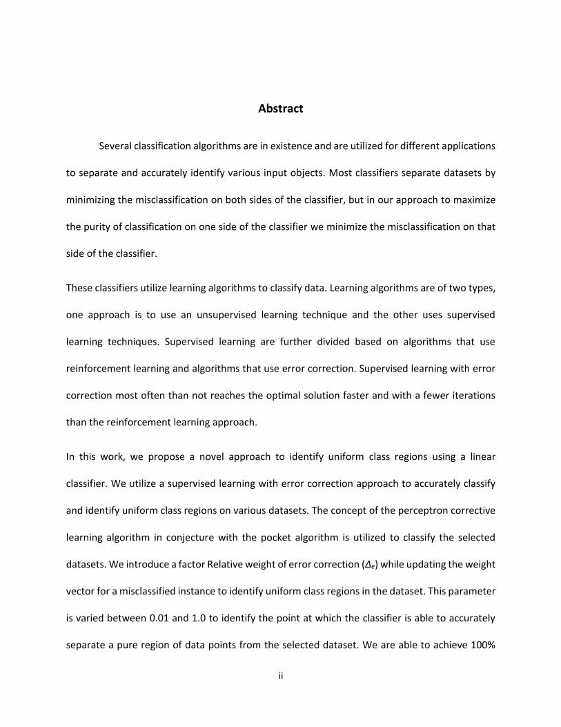
Abstract
Several classification algorithms are in existence and are utilized for different applications
to separate and accurately identify various input objects. Most classifiers separate datasets by
minimizing the misclassification on both sides of the classifier, but in our approach to maximize
the purity of classification on one side of the classifier we minimize the misclassification on that
side of the classifier.
These classifiers utilize learning algorithms to classify data. Learning algorithms are of two types,
one approach is to use an unsupervised learning technique and the other uses supervised
learning techniques. Supervised learning are further divided based on algorithms that use
reinforcement learning and algorithms that use error correction. Supervised learning with error
correction most often than not reaches the optimal solution faster and with a fewer iterations
than the reinforcement learning approach.
In this work, we propose a novel approach to identify uniform class regions using a linear
classifier. We utilize a supervised learning with error correction approach to accurately classify
and identify uniform class regions on various datasets. The concept of the perceptron corrective
learning algorithm in conjecture with the pocket algorithm is utilized to classify the selected
datasets. We introduce a factor Relative weight of error correction (∆e) while updating the weight
vector for a misclassified instance to identify uniform class regions in the dataset. This parameter
is varied between 0.01 and 1.0 to identify the point at which the classifier is able to accurately
separate a pure region of data points from the selected dataset. We are able to achieve 100%

iii
precision in classification and identification of pure region of points within the selected dataset
when a pure region exists. We provide a detailed analysis of our results on these non-linearly
separable datasets and confirm that our proposed method is able to accurately identify uniform
class regions on various datasets.

iv

v
Acknowledgement
First of all I would like to thank God for his amazing providence and his hand over my life, which
has enabled me to come so far. Next, I would like to thank my advisor Dr. Raj Bhatnagar for his
guidance and valuable feedback that has enabled me to bring this work to successful completion.
I would also like to thank Dr. Paul Talaga and Dr. Nan Niu for taking time out of their busy
schedules to be on my thesis committee.
I would like to thank my lab mates Kumar and Sambhavi for their constant support and
encouragement which has enabled me to bring out my best work. I would also like to thank my
friends Bharat, Ujwal, Suraj, Sannath, Ketan and Ankita for constantly pushing me to reach a
higher standard.
Last, but definitely not the least, I am extremely grateful to my family for always wanting the best
for me. My grandparents, Dr. Francis and Dr. Premela Samuel whose love and devotion cannot
be measured. My mother, Sasikala who has sacrificed so much for me, and is always praying for
me to succeed. My aunt Shakila, uncle Jayant and cousin Daniel who have been a second family
to me. My sister Tangela and her family for their unwavering faith in me.

vi
Table of Contents
Chapter 1: Introduction 1
1.1 Our Approach and its Benefits 2
1.2 Overview of Other Chapters 5
Chapter 2: Related Work 6
2.1 Classification Approaches 6
2.1.1 Least Mean Square Solution (LMS) 6
2.1.2 Optimal Margin Classifiers 8
2.1.3 Support Vector Network 9
2.1.4 Back Propagation Training Algorithm 10
2.2 Advantages of our Approach 11
Chapter 3: Classification Algorithm 12
3.1 Important Metrics 12
3.1.1 Entropy 12
3.1.2 Class Purity 14
3.2 Classification Approach 14
Chapter 4: Experimental Setup and Results 27
vii
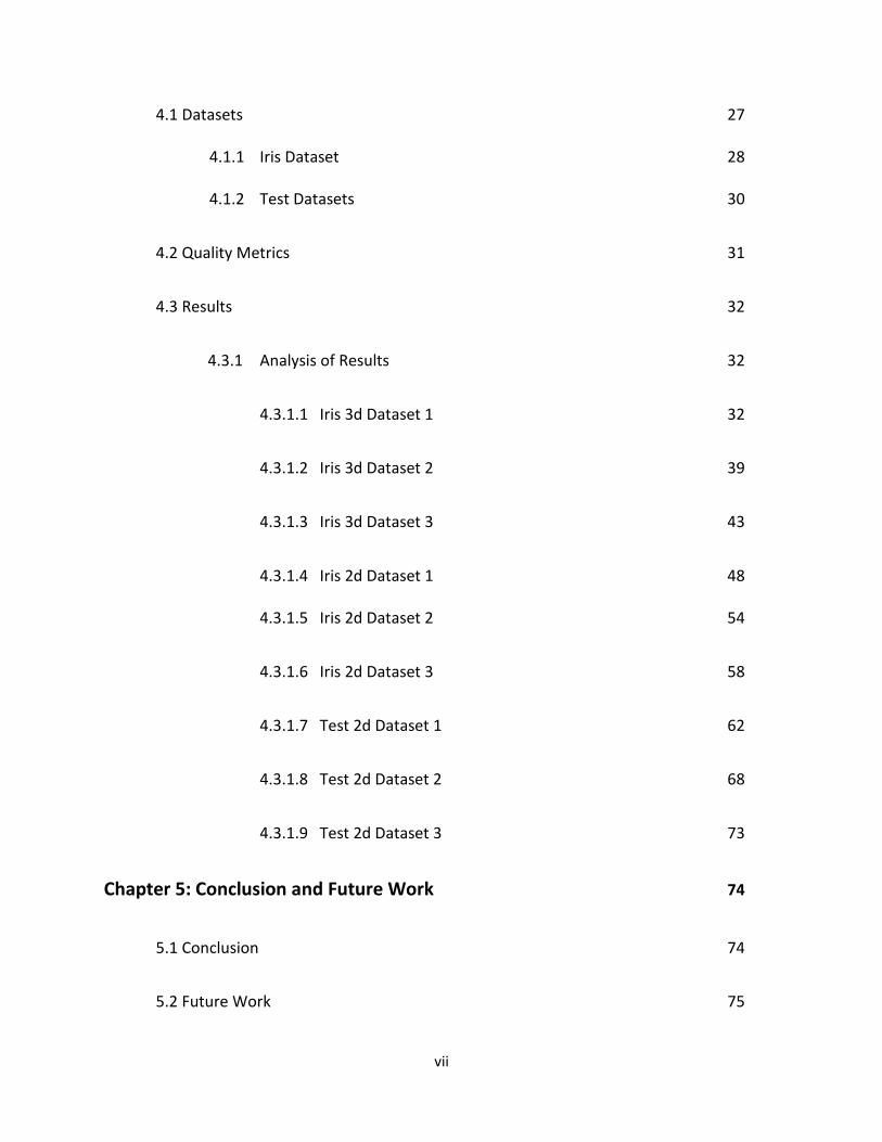
4.1 Datasets 27
4.1.1 Iris Dataset 28
4.1.2 Test Datasets 30
4.2 Quality Metrics 31
4.3 Results 32
4.3.1 Analysis of Results 32
4.3.1.1 Iris 3d Dataset 1 32
4.3.1.2 Iris 3d Dataset 2 39
4.3.1.3 Iris 3d Dataset 3 43
4.3.1.4 Iris 2d Dataset 1 48
4.3.1.5 Iris 2d Dataset 2 54
4.3.1.6 Iris 2d Dataset 3 58
4.3.1.7 Test 2d Dataset 1 62
4.3.1.8 Test 2d Dataset 2 68
4.3.1.9 Test 2d Dataset 3 73
Chapter 5: Conclusion and Future Work 74
5.1 Conclusion 74
5.2 Future Work 75

viii
References 77
ix
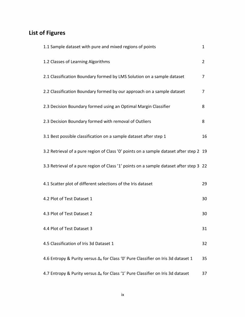
List of Figures
1.1 Sample dataset with pure and mixed regions of points 1
1.2 Classes of Learning Algorithms 2
2.1 Classification Boundary formed by LMS Solution on a sample dataset 7
2.2 Classification Boundary formed by our approach on a sample dataset 7
2.3 Decision Boundary formed using an Optimal Margin Classifier 8
2.3 Decision Boundary formed with removal of Outliers 8
3.1 Best possible classification on a sample dataset after step 1 16
3.2 Retrieval of a pure region of Class ’0’ points on a sample dataset after step 2 19
3.3 Retrieval of a pure region of Class ’1’ points on a sample dataset after step 3 22
4.1 Scatter plot of different selections of the Iris dataset 29
4.2 Plot of Test Dataset 1 30
4.3 Plot of Test Dataset 2 30
4.4 Plot of Test Dataset 3 31
4.5 Classification of Iris 3d Dataset 1 32
4.6 Entropy & Purity versus ∆e for Class ‘0’ Pure Classifier on Iris 3d dataset 1 35
4.7 Entropy & Purity versus ∆e for Class ‘1’ Pure Classifier on Iris 3d dataset 37

x
4.8 Classification of Iris 3d Dataset 2 39
4.9 Entropy & Purity versus ∆e for Class ‘0’ Pure Classifier on Iris 3d dataset 2 40
4.10 Entropy & Purity versus ∆e for Class ‘1’ Pure Classifier on Iris 3d dataset 2 41
4.11 Classification of Iris 3d Dataset 3 43
4.12 Entropy & Purity versus ∆e for Class ‘0’ Pure Classifier on Iris 3d dataset 3 44
4.13 Entropy & Purity versus ∆e for Class ‘1’ Pure Classifier on Iris 3d dataset 3 46
4.14 Classification of Iris 2d Dataset 1 48
4.15 Entropy & Purity versus ∆e for Class ‘0’ Pure Classifier on Iris 2d Dataset 1 50
4.16 Entropy & Purity versus ∆e for Class ‘1’ Pure Classifier on Iris 2d Dataset 1 52
4.17 Classification of Iris 2d Dataset 2 54
4.18 Entropy & Purity versus ∆e for Class ‘0’ Pure Classifier on Iris 2d Dataset 2 55
4.19 Entropy & Purity versus ∆e for Class ‘1’ Pure Classifier on Iris 2d Dataset 2 56
4.20 Classification of Iris 2d Dataset 3 58
4.21 Entropy & Purity versus ∆e for Class ‘0’ Pure Classifier on Iris 2d Dataset 3 59
4.22 Entropy & Purity versus ∆e for Class ‘1’ Pure Classifier on Iris 2d Dataset 3 60
4.23 Classification of Test 2d Dataset 1 62
4.24 Entropy & Purity versus ∆e for Class ‘0’ Pure Classifier on Test 2d Dataset 1 64
xi
4.25 Entropy & Purity versus ∆e for Class ‘1’ Pure Classifier on Test 2d Dataset 1 65
4.26 Class ’0’ Pure Region Removed From Test 2d Dataset 1 67
4.27 Class ’1’ Pure Region Removed From Test 2d Dataset 1 67
4.28 Second Class ‘0’ Pure Region Classifier on Test 2d Dataset 1 68
4.29 Classification of Test 2d Dataset 2 68
4.30 Entropy & Purity versus ∆e for Class ‘0’ Pure Classifier on Test 2d Dataset 2 70
4.31 Entropy & Purity versus ∆e for Class ‘1’ Pure Classifier on Test 2d Dataset 2 71
4.32 Test 2d Dataset 3 73

xii
List of Tables
1.1 An example of epoch # vs misclassified points on a sample dataset 3
4.1 Dataset description 28
4.2 Results of Main Perceptron Classifier on Iris 3d dataset 1 33
4.3 Results of Class ‘0’ Pure Classifier on Iris 3d dataset 1 36
4.4 Confusion Matrix and Accuracy of Class ‘0’ Pure Classifier on Iris 3d
dataset 1 36
4.5 Results of Class ‘1’ Pure Classifier on Iris 3d dataset 1 37
4.6 Confusion Matrix and Accuracy of Class ‘1’ Pure Classifier on Iris 3d
dataset 1 38
4.7 Results of Main Perceptron Classifier on Iris 3d dataset2 39
4.8 Results of Class ‘0’ Pure Classifier on Iris 3d dataset 2 40
4.9 Confusion Matrix and Accuracy of Class ‘0’ Pure Classifier on Iris 3d
dataset 2 41
4.10 Results of Class ‘1’ Pure Classifier on Iris 3d dataset 2 42
4.11 Confusion Matrix and Accuracy of Class ‘1’ Pure Classifier on Iris 3d
dataset 2 42
4.12 Results of Main Perceptron Classifier on Iris 3d dataset3 43
4.13 Results of Class ‘0’ Pure Classifier on Iris 3d dataset 3 44
xiii
4.14 Confusion Matrix and Accuracy of Class ‘0’ Pure Classifier on Iris 3d
dataset 3 45
4.15 Results of Class ‘1’ Pure Classifier on Iris 3d dataset 3 46
4.16 Confusion Matrix and Accuracy of Class ‘1’ Pure Classifier on Iris 3d
dataset 3 47
4.17 Results of Main Perceptron Classifier on Iris 2d dataset 1 49
4.18 Results of Class ‘0’ Pure Classifier on Iris 2d dataset 1 51
4.19 Confusion Matrix and Accuracy of Class ‘0’ Pure Classifier on Iris 2d
dataset 1 51
4.20 Results of Class ‘1’ Pure Classifier on Iris 2d dataset 1 52
4.21 Confusion Matrix and Accuracy of Class ‘1’ Pure Classifier on Iris 2d
dataset 1 53
4.22 Results of Main Perceptron Classifier on Iris 2d dataset2 54
4.23 Results of Class ‘0’ Pure Classifier on Iris 2d dataset 2 55
4.24 Confusion Matrix and Accuracy of Class ‘0’ Pure Classifier on Iris 2d
dataset 2 56
4.25 Results of Class ‘1’ Pure Classifier on Iris 2d dataset 2 57
4.26 Confusion Matrix and Accuracy of Class ‘1’ Pure Classifier on Iris 2d
dataset 2 57
4.27 Results of Main Perceptron Classifier on Iris 2d dataset3 58

xiv
4.28 Results of Class ‘0’ Pure Classifier on Iris 2d dataset 3 58
4.29 Confusion Matrix and Accuracy of Class ‘0’ Pure Classifier on Iris 2d
dataset 3 60
4.30 Results of Class ‘1’ Pure Classifier on Iris 2d dataset 3 61
4.31 Confusion Matrix and Accuracy of Class ‘1’ Pure Classifier on Iris 2d
dataset 3 61
4.32 Results of Main Perceptron Classifier on Test 2d dataset 1 63
4.33 Results of Class ‘0’ Pure Classifier on Test 2d dataset 1 64
4.34 Confusion Matrix and Accuracy of Class ‘0’ Pure Classifier on Test 2d
dataset 1 65
4.35 Results of Class ‘1’ Pure Classifier on Test 2d dataset 1 66
4.36 Confusion Matrix and Accuracy of Class ‘1’ Pure Classifier on Test 2d
dataset 1 66
4.37 Results of Main Perceptron Classifier on Test 2d dataset2 69
4.38 Results of Class ‘0’ Pure Classifier on Test 2d dataset 2 70
4.39 Confusion Matrix and Accuracy of Class ‘0’ Pure Classifier on Test 2d
dataset 2 71
4.40 Results of Class ‘1’ Pure Classifier on Test 2d dataset 2 72
4.41 Confusion Matrix and Accuracy of Class ‘1’ Pure Classifier on Test 2d

xv
dataset 2 72

xvi
List of Algorithms
1. Optimized Perceptron Corrective Learning Algorithm for Pure Class 0 Region 19
2. Optimized Perceptron Corrective Learning Algorithm for Pure Class 1 Region 22
3. Algorithm to identify number of misclassified points at the end of each epoch 23
4. Algorithm to remove pure region of Class ‘0’ points from dataset 24
5. Algorithm to remove pure region of Class ‘1’ points from dataset 25
1
Chapter 1
Introduction
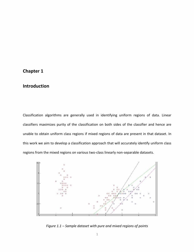
Classification algorithms are generally used in identifying uniform regions of data. Linear
classifiers maximizes purity of the classification on both sides of the classifier and hence are
unable to obtain uniform class regions if mixed regions of data are present in that dataset. In
this work we aim to develop a classification approach that will accurately identify uniform class
regions from the mixed regions on various two-class linearly non-separable datasets.
Figure 1.1 – Sample dataset with pure and mixed regions of points

2
Figure 1.1 depicts a linearly non-separable sample dataset which has pure and mixed regions of
points. The black classifier line in Figure 1.1 is the classification obtained by maximizing the
purity of points on both sides of the classifier. This classification of points is unable to identify
uniform regions of points on such datasets. Our approach of classification on such datasets is to
maximize the purity of points on a single side of the classification boundary thereby identifying
a uniform region of points on one side of the classifier. The points below the pink and above the
green classification boundaries are the uniform regions of points identified using our
classification approach.
Reinforcement learning
Supervised learning
Learning Corrective learning
Unsupervised learning
Figure 1.2 - Classes of Learning Algorithms
Figure 1.2 shows the different types of learning algorithms that are used to classify data. Our
approach utilizes the corrective learning approach to identify uniform class regions of data.
1.1 Our Approach and its Benefits
In this work we utilize a linear classifier using a supervised learning with error correction
approach to classify various two-class linearly non-separable datasets.

3
We leverage the perceptron corrective learning algorithm and the pocket algorithm to
initially obtain the best possible classification of our dataset. We determine that we
have reached the best classification of our dataset when the total number of
misclassified points on each side of our classifier does not reduce any further and it
remains constant over five consecutive epochs.
Table 1.1 – An example of epoch # vs misclassified points on a sample dataset
In Table 1.1, we determine that at Epoch #49 we have obtained the best possible
classification of our dataset. We can see that the number of misclassified points remains
consecutive over five consecutive epochs (Epoch# 45 – Epoch #49) and does not reduce
any further. Table 1.1 depicts the stopping condition of our classifier.
We then retrieve the uniform Class ‘0’ region utilizing the perceptron corrective learning
algorithm. This algorithm is used to update the error correction on the weight vector for
a misclassified Class ‘1’ instance with a factor (∆e), where ∆e is the relative weight for
error correction and has a value ranging between 0.01 – 1.0, while updating the error
correction on the weight vector for a misclassified Class ‘0’ instance in entirety. By this
approach we are able to increase the purity of Class ‘0’ points on one side of our
Epoch #
Number of
misclasssified
points
45 20
46 20
47 20
48 20
49 20
50 22
51 23

4
classifier and thus obtain a uniform Class ‘0’ region on one side of the classification
boundary.
We then retrieve the uniform Class ‘1’ region utilizing the perceptron corrective learning
algorithm. This algorithm updates the error correction on the weight vector for a
misclassified Class ‘0’ instance with a factor (∆e), where ∆e is the relative weight for error
correction and has a value ranging between 0.01 – 1.0, while updating the error
correction on the weight vector for a misclassified Class ‘1’ instance in entirety. By this
approach we are able to increase the purity of Class ‘1’ points on one side of our
classifier and thus obtain a uniform Class ‘1’ region on one side of the classification
boundary.
In our approach, we are able to overcome the limitations faced by other classifiers on datasets
which have mixed regions of points present and is able to successfully identify uniform class
regions and separate them from the mixed regions of data using the classification approach
mentioned above. We also are able to achieve 100% precision of pure points (Class ‘0’ and Class
‘1’) on one side of our classifier on 8 different linearly non-separable two-class datasets when
there exists a pure region of points in that selected dataset.
Our approach is not limited by requiring a high dimensional feature space to classify non-
separable data as is the case in the approach used while classifying data with a support vector
network. It also does not have the additional overhead of requiring many different training runs
to accurately classify data such as the back-propagation training algorithm. We bring out these
and other limitations in the approaches used in classifying non-separable datasets in chapter 2.

5
1.2 Overview of Other Chapters
Our algorithm is tested against various two-class non-separable datasets and we are able to
identify pure regions of data when they were present in the selected datasets. In chapter 2, we
introduce the classifiers in existence and validate its performance against various datasets. We
also discuss their limitations and aim to address the drawbacks with these classifiers in our
research. In chapter 3, we present our approach and justify the reasons behind the design of
our algorithm. In chapter 4, we present the results of our algorithm tested against various
linearly non-separable two-class datasets and highlight the accuracy and performance of our
classifier. In chapter 5, we conclude by providing a brief summary of the analysis of our results
and also discuss the future work in this area.

6
Chapter 2
Related Work
2.1 Classification Approaches
There has been a lot of research in the area of identifying unique approaches in classifying
separable and non-separable data. In the below section we present various existing algorithms
that utilize a supervised training approach towards separation of data and also highlight their
drawbacks.
2.1.1 Least Mean Square Solution (LMS)
The least mean square solution, a modification to the perceptron convergence solution was
introduced by Widrow and Hoff. [2] The LMS solution minimizes the mean square error
between the expected output and the actual output by using an error correction approach that
7
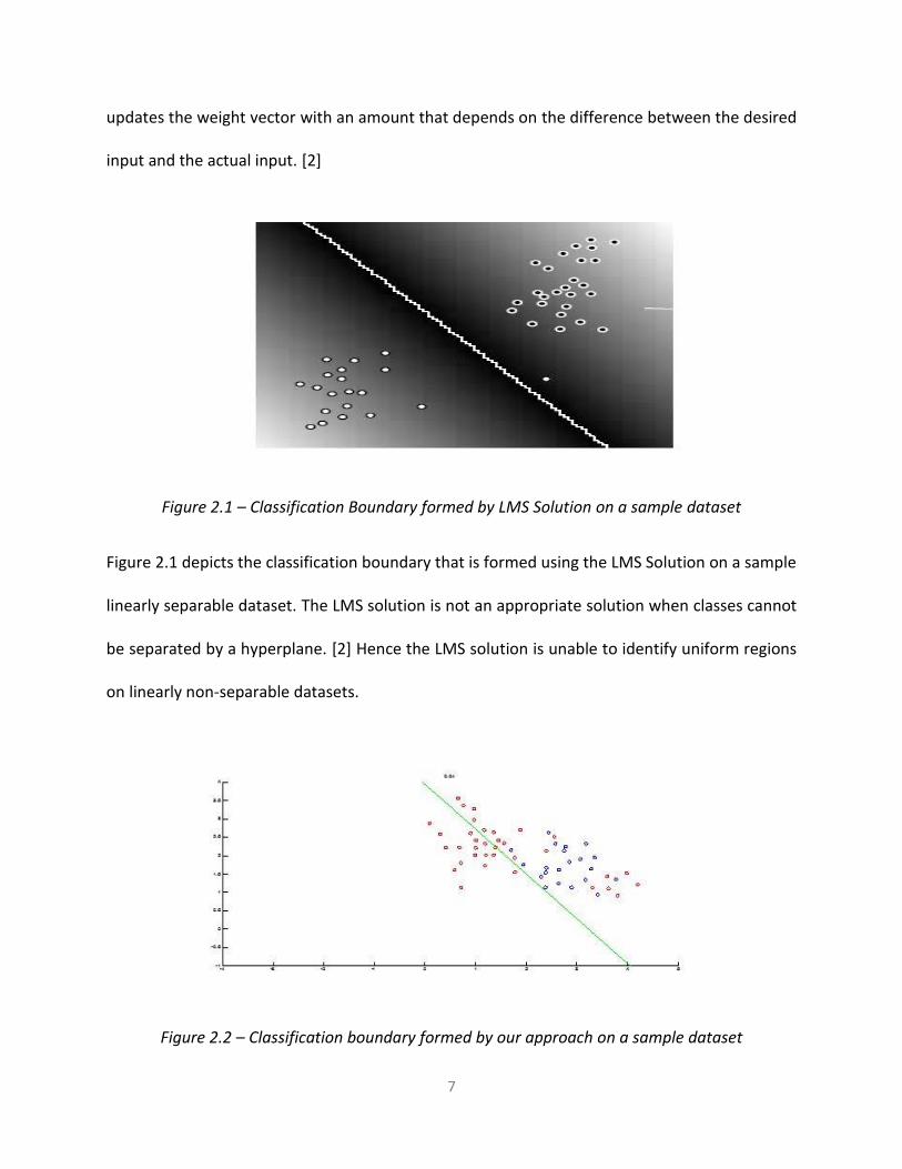
updates the weight vector with an amount that depends on the difference between the desired
input and the actual input. [2]
Figure 2.1 – Classification Boundary formed by LMS Solution on a sample dataset
Figure 2.1 depicts the classification boundary that is formed using the LMS Solution on a sample
linearly separable dataset. The LMS solution is not an appropriate solution when classes cannot
be separated by a hyperplane. [2] Hence the LMS solution is unable to identify uniform regions
on linearly non-separable datasets.
Figure 2.2 – Classification boundary formed by our approach on a sample dataset

8
Figure 2.2 depicts the classification boundary obtained using our classification approach on a
sample linearly non-separable dataset. We can see that we are able to identify a uniform
region of points (the points below the green classifier line) using our classification approach by
focusing on identification of a pure region of points on one side of the classification boundary.
2.1.2 Optimal Margin Classifiers
This algorithm is presented by Boser, Guyon and Vapnik. [3] Their approach to the classification
of the dataset maximizes the margin between the training patterns and the decision boundary.
Similar to our approach, the algorithm has also achieved better efficiency using multi layered
neural networks and has achieved errorless separation of training data when possible. It
converges to the solution faster by reducing the number of computations with the use of dual
space representation and appropriate search techniques. [3]
Figure 2.3 – Decision boundary formed using Figure 2.4 – Decision boundary an Optimal Margin Classifier formed with removal of Outliers

9
Figure 2.3 depicts the classification boundary formed using an optimal margin classifier, the
points closest to the decision boundary (points labelled ‘1’ and ‘2’) refer to the supporting
patterns and the final classification depends on these supporting patterns.
Figure 2.3 depicts the classification boundary formed by removal of an outlier from the training
data on the same dataset. We see a change in the classification boundary with the removal of
the outliers or atypical patterns from the training data.
Despite its various advantages, the Optional Margin Classifiers has proved efficient only on
linearly separable datasets and on datasets which have outliers or atypical patterns present.
This approach of maximizing the margin between the classification boundary will not work on
datasets that have overlapped distributions. Hence the optimal margin classifier is not an
appropriate solution for non-separable datasets.
2.1.3 Support Vector Network (SVM)
Support Vector Network is a learning machine implemented for two-group classification
problems. Cortes and Vapnik extended the concept of the support vector network to be trained
on non-separable data. [4]
Similar to our approach to minimize the number of misclassification errors, SVM constructs a
hyperplane that maximizes the margin to separate the data with minimal number of errors. It
achieves this by removing the minimal subset of training errors from the training data and
constructs the optimal separating hyperplane from the remainder of the training data. [4]

10
The same approach is extended for non-linear decision surfaces by the projection of the input
vectors to a higher dimensional feature space and a linear classification problem formulated on
this feature space. [4]
SVM is able to classify non-separable datasets but has the following limitations,
For non-linear decision surfaces the dimensionality of the feature space increases in size
drastically and could become very large to be accommodated.
The approach implemented for the non-linear mapping of the input vector to the higher
dimensional feature space is cumbersome. [4]
Our approach is able to build a linear classifier for non-separable datasets without the
additional overhead experienced using a SVM.
2.1.4 Back Propagation Training Algorithm
This supervised learning algorithm is a generalized form of the LMS algorithm and uses an
iterative gradient search technique to minimize the cost function of the network. The cost
function is the mean square error between the desired output and the actual output of the
multi-layer perceptron. Weights are continually adjusted after every validation until the cost
function is reduced to an acceptable value and it converges to a solution. [5]
Similar to our algorithm, it has also been tested successfully against various non-linearly
separable datasets and it uses decision regions formed by a two layer perceptron and the back
propagation approach. [5]

11
The back-propagation algorithm suffers various drawbacks while classifying non-separable
datasets,
The gradient search technique more often than not ends up finding the local minimum
instead of the desired global minimum.
The number of iterations required for convergence has been large on many cases and it
is unlikely that the convergence could be sped up due to the complex decision regions
generated by the multi-layer perceptron. [5]
2.2 Advantages of our Approach
As discussed in the above section there are various classification algorithms that use supervised
learning approaches to train and classify data. These algorithms have some drawbacks and
limitations when it comes to classifying certain datasets, in our work we aim to overcome these
limitations and identify uniform class regions on these linearly non-separable datasets.
In our approach presented in chapter 3, we introduce our algorithm to classify and identify
uniform class regions and separate them from the mixed regions of data on various two-class
non-separable datasets.

12
Chapter 3
Classification Algorithm
In this chapter we introduce our version of the optimized perceptron corrective learning
algorithm to identify uniform class regions on various two-class datasets. We provide an
explanation to our classification approach and also discuss how our algorithm can be used to
identify uniform class regions on the selected datasets. We also provide reasons behind our
algorithm’s design and illustrate its working using an example.
3.1 Important Metrics
In order to explain the design of our algorithm, we provide a brief explanation of a few key
metrics which is used in our classification approach.
3.1.1 Entropy
Entropy measures the homogeneity of a group of data points. It is calculated using the formula,
13
Entropy = - ∑ (pi) * log2 (pi), where pi = (# of Classi Points) / (Total # of points)
As entropy is being calculated for two-class datasets, it is at its maximum (1.0) when records
are equally distributed among both classes, implying least purity of points from that
classification. It is at its minimum (0.0) when all records belong to an individual class, implying
best purity of points in that classification. In our scenario we thus conclude that we have a pure
region of points when the entropy is at its minimum value.
Class Entropy
It is referred to the entropy calculated on each side of the classifier. Class Left Entropy and Class
Right Entropy are identified by the entropy calculated on the left and right side of the classifier
respectively. Class Left Entropy is calculated using the formula,
po = (# of points correctly classified left of the classifier/total # of points left of the classifier)
p1= (# of points incorrectly classified left of the classifier/total # of points left of the classifier)
Class Left Entropy = - [(p0) * log2 (p0) + (p1) * log2 (p1)]
Class Right Entropy is calculated using a similar formula for the classification on the right of the
classifier.
Total Weighted Entropy
It is defined as the weighted average of the individual class entropies. It is calculated using the
formula,

14
Total Weighted Entropy = [((# of points left of the classifier/total points) * Class Left Entropy) +
((# of points right of the classifier/total points) * Class Right Entropy)]
3.1.2 Class Purity
It refers to the purity of points on one side of the classifier. In our scenario it is evaluated by
calculating the precision of the classification on one side of the classifier, and is calculated as
the ratio of the number of points correctly classified on one side of the classifier to the total
number of points on that side of the classifier.
3.2 Classification Approach
Step 1: Identify best possible classification on the two-class dataset
In order to identify uniform class regions on various two-class datasets we leverage the
perceptron corrective learning algorithm and utilize the concept of the pocket algorithm to
initially identify the best possible classification of the dataset. The pocket algorithm stores the
best weight vector found until then by the classifier in a pocket while continuing to update the
weight vector. [6] The classifier is run until the best possible classification of the dataset is
reached, and it is achieved when the total number of misclassified points on each side of the

15
classifier does not reduce any further and remains constant over 5 consecutive epochs. An
epoch is identified as one complete iteration of the classifier.
The perceptron corrective learning algorithm accelerates convergence to a solution with a
fewer number of iterations (epochs) than the perceptron learning algorithm by normalizing the
input weight vector and also providing an improvement on error correction of the weight
vector. [1]
The error (delta) is defined as, δ = - (wt . x). If a Class ‘1’ instance is classified erroneously, the
new weight vector is calculated using the formula, wt+1 = wt + ((δ + ε)/ ||x|| ^ 2) . x
Where ||x|| is a normalized input vector and ε denotes a very small number which provides a
guarantee that the new weight vector just manages to skip the border of region with a higher
error. When a Class ’0’ instance is classified erroneously, the weight vector is updated similarly
except that we use the correction factor of (δ - ε) instead of (δ + ε). [1]
The final weight vector (wt) obtained by the perceptron corrective learning algorithm after step
1 is the ‘Main Perceptron Classifier’ which will be explained in detail in chapter 4. This is the
best possible classification of dataset achieved so far and it (wt) will be used as the initial weight
vector to further identify the uniform class regions in the given dataset (step 2 and step 3 of our
approach). The green line in Figure 3.1 depicts the main perceptron classifier on a sample two-
class dataset.

16
Figure 3.1 – Best possible classification on a sample two-class dataset after step 1
Step 2: Identify uniform Class ‘0’ region on the two-class dataset
The initial weight vector w0 is initialized to the final weight vector wt which is the output
obtained at the end of step 1 of the classifier. We then run an optimized version of the
perceptron corrective learning algorithm (Algorithm 1) to determine the uniform Class ‘0’
region in the dataset. We cap the number of epochs (iterations) that the classifier will run to
five hundred which enables the classifier to exit in case it is unable to identify a uniform Class
‘0’ region in this dataset.

17
As mentioned in step 1, delta (δ), the error correction is used to update the weight vector, and
if a Class ‘0’ instance is classified erroneously, the new weight vector is calculated using the
formula,
wt+1 = wt + ((δ - ε)/ ||x|| ^ 2) . x [1]
If a Class ‘1’ instance is classified erroneously, the new weight vector is calculated using the
formula,
wt+1 = wt + ∆e * ((δ + ε)/ ||x|| ^ 2) . x , where ∆e is the Relative weight of error correction
for updating the weight vector for misclassified Class ‘1’ points.
We vary the values of ∆e from 0.01 – 1.0 until the Entropy on one side of the classifier reaches
zero. This implies that the weight vector is updated only by a fraction (∆e) of the expected error
correction value for a misclassified Class ‘1’ instance while the weight vector is updated in
entirety with the error correction value for a misclassified Class ‘0’ instance, thus enabling the
purity of points on one side of the classifier to increase while the purity of points on the other
side of the classifier decreases. Hence we are able to retrieve a pure region of Class ‘0’ points
on that side of the classifier.
The final weight vector (wt) obtained at the end of step 2 is referred to as the Class ‘0’ Pure
Region Classifier which is explained in detail in chapter 4 and the points below this classifier are

18
the pure region of Class ‘0’ points. The black line in Figure 3.2 depicts the Class ’0’ pure region
classifier on a sample two-class dataset.
Input: w0 (initial weight vector) = wt (final weight vector output in Step 1),
x € (Class 1 U Class 0).
Output: final weight vector wt which provides a uniform Class ‘0’ region on one
side of the classifier.
1) w0 <- wt
2) N <- 500 (cap on number of Epochs), stop <- false, epochCtr <- 1 (Epoch #)
3) while stop is equal to false and epochCtr less than equal to N
4) for t is equal to 1, t less than equal to total points, increment t
5) Error δ <- - (wt . x)
6) if x € Class ‘0’ and wt . x >= 0,
7) wt+1 <- wt + ((δ - ε)/ ||x||^ 2) . x
8) end if
9) if x € Class ‘1’ and wt . x <= 0,
10) wt+1 <- wt + ∆e * ((δ + ε)/ ||x||^ 2) . x
11) end if

19
Algorithm 1 - Optimized Perceptron Corrective Learning Algorithm for Uniform Class 0 Region
Figure 3.2 - Retrieval of uniform Class ’0’ region on a sample two-class dataset after step 2
12) end for
13) if the number of misclassified points does not reduce further and is constant
over 5 epochs and Class Left Entropy is equal to 0.0
14) stop <- true
15) end if
16) epochCtr <- epochCtr + 1
17) end while

20
Step 3: Identify uniform Class ‘1’ region on the two-class dataset
The initial weight vector w0 is initialized to the final weight vector wt which is the output
obtained at the end of Step 1 of the classifier. We then run an optimized version of the
perceptron corrective learning algorithm (Algorithm 2) to determine the uniform Class ’1’
region from the dataset. We cap the number of epochs (iterations) that the classifier will run to
five hundred which enables the classifier to exit in case it is unable identify uniform Class ‘1’
region in this dataset.
As mentioned in Step 1, delta (δ), the error correction is used to update the weight vector, and
if a Class ‘1’ instance is classified erroneously, the new weight vector is calculated using the
formula,
wt+1 = wt + ((δ + ε)/ ||x|| ^ 2) . x [1]
If a Class ‘0’ instance is classified erroneously, the new weight vector is calculated using the
formula,
wt+1 = wt + ∆e * ((δ - ε)/ ||x|| ^ 2) . x, where ∆e is the relative weight of Error Correction
for updating the weight vector for Class ‘0’ points.
We vary the values of ∆e from 0.01 – 1.0 until the Entropy on one side of the classifier reaches
zero. This implies that the weight vector is updated only by a fraction (∆e) of the expected error
correction value for a misclassified Class ‘0’ instance while the weight vector is updated in
entirety with the error correction value for a misclassified Class ‘1’ instance, thus enabling the
purity of points on one side of the classifier to increase while the purity of points on the other

21
side of the classifier decreases. Hence we are able to retrieve a pure region of Class ‘1’ points
on that side of the classifier.
The final weight vector (wt) obtained at the end of Step 3 is referred to as the Class ‘1’ Pure
Region Classifier and the points above this classifier indicates the pure region of Class ‘1’ points.
The pink line in Figure 3.3 depicts the Class ’1’ pure region classifier on a sample two-class
dataset.
Input: w0 (initial weight vector) = wt (final weight vector output in Step 1),
x € (Class 1 U Class 0).
Output: final weight vector wt which provides a uniform Class ‘1’ region on one
side of the classifier.
1) w0 <- wt
2) N <- 500 (cap on number of Epochs), stop <- false, epochCtr <- 1 (Epoch #)
3) while stop is equal to false and epochCtr less than equal to N
4) for t is equal to 1, t less than equal to total points, increment t
5) Error δ <- - (wt . x)
6) if x € Class ‘1’ and wt . x <= 0,
7) wt+1 <- wt + ((δ + ε)/ ||x||^ 2) . x
8) end if
9) if x € Class ‘0’ and wt . x >= 0,
10) wt+1 <- wt + ∆e * ((δ - ε)/ ||x||^ 2) . x

22
Algorithm 2 - Optimized Perceptron Corrective Learning Algorithm for Uniform Class 1 Region
Figure 3.3 - Retrieval of a uniform Class ’1’ region on a sample two-class dataset after step 3
11) end if
12) end for
13) if the number of misclassified points does not reduce further and is
constant over 5 epochs and Class Right Entropy is equal to 0.0
14) stop <- true
15) end if
16) epochCtr <- epochCtr + 1
17) end while

23
We detail the process used to identify the number of misclassified points on each side of the
classifier at end of each epoch in the below Algorithm.
Algorithm 3 – Algorithm to identify number of misclassified points at the end of each epoch
Input: wt (updated weight vector after error correction), P € (Class 1 U Class 0)
Output: m, number of misclassified points at the end of each epoch
1) w1 <- wt (1), w2 <- wt (2), w3 <- wt (3), m <- 0
2) for i is equal to 1, i less than equal to total points, increment i
3) sum <- (w1 * x + w2 * y + w3) / w2,
where x, y are the x and y co-ordinates of Point P
4) if sum >= 0 and P € Class ‘0’
5) increment m
6) end if
7) if sum <= 0 and P € Class ‘1’
8) increment m
9) end if
10) end for

24
Step 4: Remove identified uniform regions of points from the dataset
Once we have identified uniform regions of data in the dataset as explained in Step 2 and 3, we
remove these data points from our dataset to verify if there are any other identifiable uniform
regions of data in our dataset.
We first update our dataset by removing all the points (Class ‘0’) below the Class ‘0’ Pure
Region Classifier which is obtained in Step 2. We detail the approach to remove these points in
Algorithm 4, this removes the identified pure region of Class ‘0’ points from our dataset.
Input: wt (final weight vector output in Step 2), P € (Class 1 U Class 0).
Output: P’ € (Class 1 U Class 0) with Class ‘0’ pure region of points removed
1) w1 <- wt (1), w2 <- wt (2), w3 <- wt (3)
2) for i is equal to 1, i less than equal to total points, increment i
3) sum <- (w1 * x + w2 * y + w3) / w2,
where x, y are the x and y co-ordinates of Point P
4) if sum <= 0 and P € Class ‘0’
5) continue
7) else
8) P’ <- P
9) end if
10) end for

25
Algorithm 4 – Algorithm to remove pure region of Class ‘0’ points from dataset
We then update our dataset by also removing all the points (Class ‘1’) above the Class ‘1’ Pure
Region Classifier which is obtained in Step 3. We detail the approach to remove these points in
Algorithm 5, this removes the identified pure region of Class ‘1’ points from our dataset.
Algorithm 5 – Algorithm to remove pure region of Class ‘1’ points from dataset
Input: wt (final weight vector output in Step 3), P’ € (Class 1 U Class 0) (points with
Class ‘0’ pure region removed, output of Algorithm 3.3).
Output: P’’ € (Class 1 U Class 0) with Class ‘1’ pure region of points removed
1) w1 <- wt (1), w2 <- wt (2), w3 <- wt (3)
2) for i is equal to 1, i less than equal to total points, increment i
3) sum <- (w1 * x + w2 * y + w3) / w2,
where x, y are the x and y co-ordinates of Point P’
4) if sum >= 0 and P’ € Class ‘1’
5) continue
7) else
8) P’’ <- P’
9) end if
10) end for

26
Step 5: Run step 2 and step 3 until no more uniform regions (Class ‘0’ and Class ‘1’) can be
retrieved from the dataset
We then re-run Step 2 and Step 3 to verify if we would be able to identify any more uniform
regions of data from our dataset, else we stop the classification process.

27
Chapter 4
Experimental Setup and Results
4.1 Datasets
Iris dataset was selected from UCI’s machine learning data repository [7], three additional two-
class datasets were created. Detailed information regarding the datasets is provided in Table
4.1.

28
S. No
Dataset # of
instances # of
attributes Attributes names
Attribute types
# of class values
1 Iris 3d Dataset 1 150 3 Sepal Length, Sepal Width, Petal Length
Real 3
2 Iris 3d Dataset 2 150 3 Sepal Length, Sepal Width, Petal Width
Real 3
3 Iris 3d Dataset 3 150 3 Sepal Length, Petal Length, Petal Width
Real 3
4 Iris 2d Dataset 1 150 2 Petal Length, Sepal
Width Real 3
5 Iris 2d Dataset 2 150 2 Petal Width, Petal
Length Real 3
6 Iris 2d Dataset 3 150 2 Sepal Width, Petal
Width Real 3
7 Test 2d Dataset 1 97 2 X abscissa, Y ordinate
Real 2
8 Test 2d Dataset 2 123 2 X abscissa, Y ordinate
Real 2
9 Test 2d Dataset 3 72 2 X abscissa, Y ordinate
Real 2
Table 4.1 – Dataset description
4.1.1 Iris Dataset
Figure 4.1 depicts a plot of different views of the Iris dataset, it is a three class dataset. The
class labels are setosa, versicolor and virginica where each class refers to a type of iris plant.
The dataset contains fifty instances from each of these classes, class setosa is linearly separable
from class versicolor and class virginica, class versicolor and class virginica are not linearly
separable from each other. The dataset has four numeric attributes namely sepal length, sepal
width, petal length and petal width. [8]

29
Figure 4.1 - Scatter plot of different selections of the Iris dataset [9]
We create a two-class dataset by considering instances from Class setosa and Class versicolor as
Class ‘0’ and instances from Class virginica as Class ‘1’. Six different views of the two-class Iris
dataset is created by selection of different combinations of the attributes of the Iris dataset.
Table 4.1 shows various combinations of two and three attributes selected from the Iris dataset
which in turn provides two dimensional and three dimensional two-class datasets respectively.

30
4.1.2 Test Datasets
We created three two-class datasets. These datasets contain two classes which have varied
number of instances each. Figure 4.2, 4.3 and 4.4 depicts these created datasets.
Figure 4.2 - Plot of Test Dataset 1
Figure 4.3 - Plot of Test Dataset 2

31
Figure 4.4 - Plot of Test Dataset 3
4.2 Quality Metrics
We use the following metrics to measure the accuracy of our classifier,
Precision: It is defined as the fraction of the identified class instances that are relevant. In our
scenario it indicates the fraction of instances that are correctly classified on one side of the
classifier (class purity) and is calculated as the ratio of the number of instances correctly
classified instances on one side of the classifier to the total number of instances on that side of
the classifier.
Precision = (# of instances correctly classified as Class ‘x’) / (# of instances classified as Class ‘x’)
Recall: It is defined as the fraction of relevant class instances that are identified by the classifier.
It is calculated as the ratio of the number of instances of Class ‘x’ that are correctly classified to
the total number of instances of Class ‘x’. It is calculated using the formula,

32
Recall = (# of instances correctly classified as Class ‘x’) / (total # of instances of Class ‘x’)
F-Measure: It is refers to the harmonic mean of precision and recall. It is calculated using the
formula,
F-Measure = (2 * Precision * Recall) / (Precision + Recall)
4.3 Results
4.3.1 Analysis of Results
4.3.1.1 Iris 3d Dataset 1
Figure 4.5 - Classification of Iris 3d Dataset 1
In this run of the Iris dataset three out of the four attributes are selected namely Sepal Length,
Sepal Width and Petal Length, and are given by the x, y and z axis respectively in the Figure 4.5.
Class Setosa and Class Versicolor represent Class ‘0’ points and Class Virginica represent Class
3 3.5 4 4.5 5 5.5 6 6.5 7 7.5 8
1
2
3
4
5
1
2
3
4
5
6
7
Sepal Width
Iris Dataset - 3D - Run 1 - SLvSWvPL
Sepal Length
Pet
al L
engt
h
Main Perceptron ClassifierClass 0 Pure Region ClassifierClass 1 Pure Region Classifier

33
‘1’ points. They are identified by the red and blue dots respectively in Figure 4.5. There are
three classifier planes shown in Figure 4.5, the Main Perceptron Classifier, Class 0 Pure Region
Classifier and Class 1 Pure Region classifier and are identified by the green, black and pink
planes respectively. The points below the Class 0 Pure Region Classifier represent the pure
region of Class ‘0’ points. The points above the Class 1 Pure Region classifier represent the pure
region of Class ‘1’ points.
The perceptron corrective learning algorithm is initially run against this selection of the Iris
dataset with a random initial weight vector. As discussed in chapter 3, we utilize the concept of
the pocket algorithm to classify the dataset and the classifier is run until the best possible
classification of the dataset is reached. It is determined that the best possible classification has
been reached by the pocket algorithm and when the total number of misclassified points on
each side of the classifier does not reduce further and remains constant over five consecutive
epochs. This classifier plane is determined to be the Main Perceptron Classifier (green plane in
Figure 4.5). As discussed in chapter 3, the final weight vector of this plane is used as the initial
weight vector for determining the pure regions of data which can be identified as the points
below and above the Class 0 Pure Region Classifier and Class 1 Pure Region Classifier
respectively.
Main Perceptron Classifier
Class Left
Entropy
Class Right
Entropy
Total Weighted Entropy
Number of Epochs to
Classify
Total Time taken to Run Classifier (in
seconds)
w1 w2 w3 w4
0.08 0.54 0.26 42 14.80 0.91 0.41 -1.40 -0.12
34
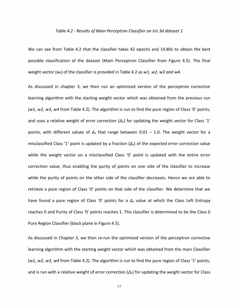
Table 4.2 - Results of Main Perceptron Classifier on Iris 3d dataset 1
We can see from Table 4.2 that the classifier takes 42 epochs and 14.80s to obtain the best
possible classification of the dataset (Main Perceptron Classifier from Figure 4.5). The final
weight vector (wt) of the classifier is provided in Table 4.2 as w1, w2, w3 and w4.
As discussed in chapter 3, we then run an optimized version of the perceptron corrective
learning algorithm with the starting weight vector which was obtained from the previous run
(w1, w2, w3, w4 from Table 4.2). The algorithm is run to find the pure region of Class ‘0’ points,
and uses a relative weight of error correction (∆e) for updating the weight vector for Class ‘1’
points, with different values of ∆e that range between 0.01 – 1.0. The weight vector for a
misclassified Class ‘1’ point is updated by a fraction (∆e) of the expected error correction value
while the weight vector on a misclassified Class ‘0’ point is updated with the entire error
correction value, thus enabling the purity of points on one side of the classifier to increase
while the purity of points on the other side of the classifier decreases. Hence we are able to
retrieve a pure region of Class ‘0’ points on that side of the classifier. We determine that we
have found a pure region of Class ‘0’ points for a ∆e value at which the Class Left Entropy
reaches 0 and Purity of Class ‘0’ points reaches 1. This classifier is determined to be the Class 0
Pure Region Classifier (black plane in Figure 4.5).
As discussed in Chapter 3, we then re-run the optimized version of the perceptron corrective
learning algorithm with the starting weight vector which was obtained from the main Classifier
(w1, w2, w3, w4 from Table 4.2). The algorithm is run to find the pure region of Class ‘1’ points,
and is run with a relative weight of error correction (∆e) for updating the weight vector for Class
35
‘0’ points, with different values of ∆e that range between 0.01 – 1.0. The weight vector for a
misclassified Class ‘0’ point is updated by a fraction (∆e) of the expected error correction value
while the weight vector on a misclassified Class ‘1’ point is updated with the entire error
correction value, thus enabling the purity of points on one side of the classifier to increase
while the purity of points on the other side of the classifier decreases. We determine that we
have found a pure region of Class ‘1’ points for a ∆e value for which the Class Right Entropy
reaches 0 and Purity of Class ‘1’ points reaches 1. This classifier is determined to be the Class 1
Pure Region Classifier (pink plane in Figure 4.5).
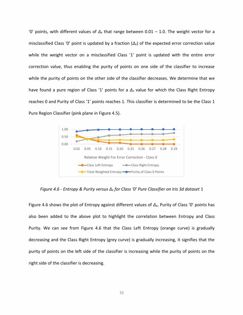
Figure 4.6 - Entropy & Purity versus ∆e for Class ‘0’ Pure Classifier on Iris 3d dataset 1
Figure 4.6 shows the plot of Entropy against different values of ∆e, Purity of Class ‘0’ points has
also been added to the above plot to highlight the correlation between Entropy and Class
Purity. We can see from Figure 4.6 that the Class Left Entropy (orange curve) is gradually
decreasing and the Class Right Entropy (grey curve) is gradually increasing, it signifies that the
purity of points on the left side of the classifier is increasing while the purity of points on the
right side of the classifier is decreasing.
0.00
0.50
1.00
0.02 0.05 0.10 0.15 0.20 0.25 0.26 0.27 0.28 0.29
Relative Weight For Error Correction - Class 0
Class Left Entropy Class Right Entropy
Total Weighted Entropy Purity of Class 0 Points

36
Class 0 Pure Classifier
Class 1 Correction
Class Left
Entropy
Class Right
Entropy
Total Weighted Entropy
Purity of Class 0 Points
Number of Epochs to Classify
Total Time taken to Run Classifier
(in seconds)
0.02 0.60 0.19 0.51 0.85 500 20.04
0.05 0.36 0.35 0.35 0.93 500 20.02
0.10 0.20 0.46 0.29 0.97 500 19.55
0.15 0.09 0.59 0.28 0.99 500 19.51
0.20 0.09 0.62 0.29 0.99 500 19.78
0.25 0.00 0.68 0.28 1.00 201 7.95
0.26 0.00 0.68 0.28 1.00 342 13.56
0.27 0.00 0.68 0.28 1.00 185 7.72
0.28 0.00 0.68 0.28 1.00 131 4.45
0.29 0.00 0.76 0.32 1.00 35 1.62
Table 4.3 - Results of Class ‘0’ Pure Classifier on Iris 3d dataset 1
We can also see from Figure 4.6 and Table 4.3 that when the Class Left Entropy reaches its
minimum value (0.0) at ∆e = 0.25 the purity of Class ‘0’ points is at its maximum value (1.0). We
have now obtained a pure region of Class ‘0’ points at this ∆e value.
Table 4.4 - Confusion Matrix and Accuracy of Class ‘0’ Pure Classifier on Iris 3d dataset 1
Table 4.4 provides a tabulation of the count of the number of class instances correctly and
incorrectly predicted as the pure class (class ‘0’) and mixed class (class ‘0’ and class ‘1’)
respectively by the Class ‘0’ Pure Region Classifier and is known as a confusion matrix. Precision,
recall and F-measure values are also provided to highlight the accuracy of the classifier.
PURE CLASS MIXED CLASS PRECISION 1.00
PURE CLASS 89 11 RECALL 0.89
MIXED CLASS 0 50 F-MEASURE 0.94
Predicted Class
Actual Class

37
Figure 4.7 - Entropy & Purity versus ∆e for Class ‘1’ Pure Classifier on Iris 3d dataset 1
Figure 4.7 shows the plot of Entropy against different values of ∆e, Purity of Class ‘1’ points has
also been added to the above plot to highlight the correlation between Entropy and Class
Purity. We can see from Figure 4.7 that the Class Right Entropy (grey curve) is gradually
decreasing and the Class Left Entropy (orange curve) is gradually increasing, it signifies that the
purity of points on the right side of the classifier is increasing while the purity of points on the
left side of the classifier is decreasing.
0
0.2
0.4
0.6
0.8
1
0.02 0.05 0.1 0.15 0.2 0.25 0.26 0.27 0.28 0.29
Relative Weight For Error Correction - Class 1Class Left Entropy Class Right Entropy
Total Weighted Entropy Purity of Class 1 Points
Class 1 Pure Classifier
Class 0 Correction
Class Left Entropy
Class Right Entropy
Total Weighted Entropy
Purity of Class 1 Points
Number of Epochs to Classify
Total Time taken to Run Classifier
(in seconds)
0.02 0.08 0.54 0.26 0.88 500 20.31
0.05 0.08 0.54 0.26 0.88 500 20.69
0.10 0.08 0.54 0.26 0.88 500 20.48
0.15 0.08 0.54 0.26 0.88 500 21.95
0.20 0.08 0.54 0.26 0.88 500 20.40
0.25 0.75 0.00 0.63 1.00 454 19.05
0.26 0.75 0.00 0.63 1.00 437 17.85
0.27 0.75 0.00 0.63 1.00 394 16.48
0.28 0.75 0.00 0.63 1.00 357 14.93
0.29 0.75 0.00 0.63 1.00 347 14.36

38
Table 4.5 - Results of Class ‘1’ Pure Classifier on Iris 3d dataset 1
We can also see from Figure 4.7 and Table 4.5 that when the Class Right Entropy reaches its
minimum value (0.0) at ∆e = 0.25, the purity of Class ‘1’ points is at its maximum value (1.0). We
have now obtained a pure region of Class ‘1’ points at this ∆e value.
Table 4.6 - Confusion Matrix and Accuracy of Class ‘1’ Pure Classifier on Iris 3d dataset 1
Table 4.6 provides a tabulation of the count of the number of class instances correctly and
incorrectly predicted as the pure class (class ‘1’) and mixed class (class ‘1’ and class ‘0’)
respectively by the Class ‘1’ Pure Region Classifier and is known as a confusion matrix. Precision,
recall and F-measure values are also provided to highlight the accuracy of the classifier.
PURE CLASS MIXED CLASS PRECISION 1.00
PURE CLASS 23 27 RECALL 0.46
MIXED CLASS 0 100 F-MEASURE 0.63
Predicted Class
Actual Class
39
4.3.1.2 Iris 3d Dataset 2
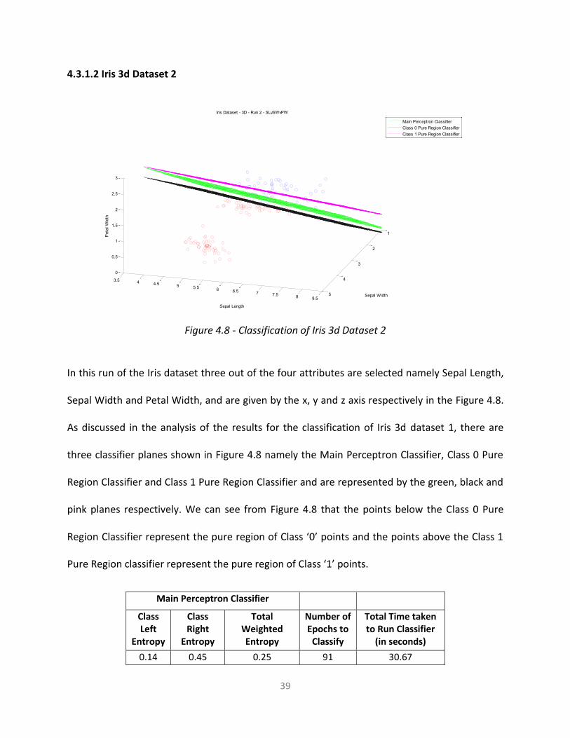
Figure 4.8 - Classification of Iris 3d Dataset 2
In this run of the Iris dataset three out of the four attributes are selected namely Sepal Length,
Sepal Width and Petal Width, and are given by the x, y and z axis respectively in the Figure 4.8.
As discussed in the analysis of the results for the classification of Iris 3d dataset 1, there are
three classifier planes shown in Figure 4.8 namely the Main Perceptron Classifier, Class 0 Pure
Region Classifier and Class 1 Pure Region Classifier and are represented by the green, black and
pink planes respectively. We can see from Figure 4.8 that the points below the Class 0 Pure
Region Classifier represent the pure region of Class ‘0’ points and the points above the Class 1
Pure Region classifier represent the pure region of Class ‘1’ points.
3.5 4 4.5 5 5.5 6 6.5 7 7.5 8 8.5
1
2
3
4
5
0
0.5
1
1.5
2
2.5
3
Sepal Width
Iris Dataset - 3D - Run 2 - SLvSWvPW
Sepal Length
Pet
al W
idth
Main Perceptron ClassifierClass 0 Pure Region ClassifierClass 1 Pure Region Classifier
Main Perceptron Classifier
Class Left
Entropy
Class Right
Entropy
Total Weighted Entropy
Number of Epochs to
Classify
Total Time taken to Run Classifier
(in seconds)
0.14 0.45 0.25 91 30.67

40
Table 4.7 - Results of Main Perceptron Classifier on Iris 3d dataset 2
We can see from Table 4.7 that the classifier takes 91 epochs and 30.67s to obtain the best
possible classifier (Main Perceptron Classifier from Figure 4.8).
Figure 4.9 - Entropy & Purity versus ∆e for Class ‘0’ Pure Classifier on Iris 3d dataset 2
As discussed in the analysis of the results for the classification of Iris 3d dataset 1, we can see
from Figure 4.9 that the Class Left Entropy (orange curve) is gradually decreasing and the Class
Right Entropy (grey curve) is gradually increasing which is an indication that the purity of points
on the left side of classifier is increasing.
Class 0 Pure Classifier
Class 1 Correction
Class Left Entropy
Class Right Entropy
Total Weighted Entropy
Purity of Class 0 Points
Number of Epochs to Classify
Total Time taken to Run Classifier
(in seconds)
0.02 0.24 0.00 0.16 0.96 500 18.87
0.05 0.24 0.25 0.24 0.96 500 20.91
0.10 0.00 0.58 0.22 1.00 7 0.35
0.11 0.00 0.58 0.22 1.00 7 0.36
0.12 0.00 0.65 0.26 1.00 7 0.38
0.00
0.20
0.40
0.60
0.80
1.00
0.05 0.10 0.11 0.12 0.13 0.14Relative Weight For Error Correction - Class 0
Class Left Entropy Class Right Entropy
Total Weighted Entropy Purity of Class 0 Points

41
0.13 0.00 0.65 0.26 1.00 7 0.35
0.14 0.00 0.68 0.28 1.00 7 0.36
Table 4.8 - Results of Class ‘0’ Pure Classifier on Iris 3d dataset 2
We can also see from Figure 4.9 and Table 4.8 that when the Class Left Entropy reaches its
minimum value (0.0) at ∆e = 0.25, the purity of Class ‘0’ points is at its maximum value (1.0). We
have now obtained a pure region of Class ‘0’ points at this ∆e value.
Table 4.9 - Confusion Matrix and Accuracy of Class ‘0’ Pure Classifier on Iris 3d dataset 2
As discussed in the analysis of the results for the classification of Iris 3d dataset 1, Table 4.9
provides a tabulation of the count of the number of class instances correctly and incorrectly
predicted by the Class ‘0’ Pure Region Classifier and is known as a confusion matrix. Precision,
recall and F-measure values are also provided to highlight the accuracy of the classifier.
Figure 4.10 - Entropy & Purity versus ∆e for Class ‘1’ Pure Classifier on Iris 3d dataset 2
PURE CLASS MIXED CLASS PRECISION 1.00
PURE CLASS 92 8 RECALL 0.92
MIXED CLASS 0 50 F-MEASURE 0.96
Predicted Class
Actual Class
0
0.2
0.4
0.6
0.8
1
0.02 0.03 0.04 0.05 0.06Relative Weight For Error Correction - Class 1
Class Left Entropy Class Right Entropy
Total Weighted Entropy Purity of Class 1 Points

42
As discussed in the analysis of the results for the classification of Iris 3d dataset 1, we can see
from Figure 4.10 that the Class Right Entropy (grey curve) is at the minimum value (0.0) which
indicates a pure region of points on the right side of the classifier.
Class 1 Pure Classifier
Class 0 Correction
Class Left Entropy
Class Right Entropy
Total Weighted Entropy
Purity of Class 1 Points
Number of Epochs to Classify
Total Time taken to Run Classifier
(in seconds)
0.02 0.58 0.00 0.45 1 18 0.80
0.03 0.58 0.00 0.45 1 18 0.78
0.04 0.58 0.00 0.45 1 18 0.71
0.05 0.58 0.00 0.45 1 18 0.81
0.06 0.58 0.00 0.45 1 18 0.82
Table 4.10 - Results of Class ‘1’ Pure Classifier on Iris 3d dataset 2
We can also see from Figure 4.10 and Table 4.10 that when the Class Right Entropy reaches its
minimum value (0.0) at ∆e = 0.02, the purity of Class ‘1’ points is at its maximum value (1.0). We
have now obtained a pure region of Class ‘1’ points at this ∆e value.
Table 4.11 - Confusion Matrix and Accuracy of Class ‘1’ Pure Classifier on Iris 3d dataset 2
As discussed in the analysis of the results for the classification of Iris 3d dataset 1, Table 4.11
provides a tabulation of the count of the number of class instances correctly and incorrectly
predicted by the Class ‘1’ Pure Region Classifier and is known as a confusion matrix. Precision,
recall and F-measure values are also provided to highlight the accuracy of the classifier.
PURE CLASS MIXED CLASS PRECISION 1.00
PURE CLASS 34 16 RECALL 0.68
MIXED CLASS 0 100 F-MEASURE 0.81
Predicted Class
Actual Class
43
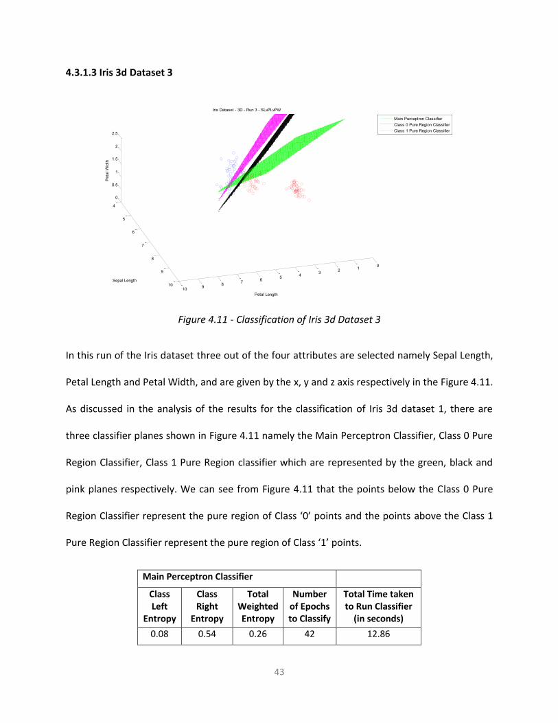
4.3.1.3 Iris 3d Dataset 3
Figure 4.11 - Classification of Iris 3d Dataset 3
In this run of the Iris dataset three out of the four attributes are selected namely Sepal Length,
Petal Length and Petal Width, and are given by the x, y and z axis respectively in the Figure 4.11.
As discussed in the analysis of the results for the classification of Iris 3d dataset 1, there are
three classifier planes shown in Figure 4.11 namely the Main Perceptron Classifier, Class 0 Pure
Region Classifier, Class 1 Pure Region classifier which are represented by the green, black and
pink planes respectively. We can see from Figure 4.11 that the points below the Class 0 Pure
Region Classifier represent the pure region of Class ‘0’ points and the points above the Class 1
Pure Region Classifier represent the pure region of Class ‘1’ points.
4
5
6
7
8
9
10
012345678910
0
0.5
1
1.5
2
2.5
Petal Length
Iris Dataset - 3D - Run 3 - SLvPLvPW
Sepal Length
Pet
al W
idth
Main Perceptron ClassifierClass 0 Pure Region ClassifierClass 1 Pure Region Classifier
Main Perceptron Classifier
Class Left
Entropy
Class Right
Entropy
Total Weighted Entropy
Number of Epochs to Classify
Total Time taken to Run Classifier
(in seconds)
0.08 0.54 0.26 42 12.86

44
Table 4.12 - Results of Main Perceptron Classifier on Iris 3d dataset 3
We can see from Table 4.12 that the classifier takes 42 epochs and 12.86s to obtain the best
possible classifier (Main Perceptron Classifier from Figure 4.11).
Figure 4.12 - Entropy & Purity versus ∆e for Class ‘0’ Pure Classifier on Iris 3d dataset 3
As discussed in the analysis of the results for the classification of Iris 3d dataset 1, we can see
from Figure 4.12 that the Class Left Entropy (orange curve) is gradually decreasing and the Class
Right Entropy (grey curve) is gradually increasing which is an indication that the purity of points
on the left side of the classifier is increasing.
Class 0 Pure Classifier
Class 1 Correction
Class Left
Entropy
Class Right
Entropy
Total Weighted Entropy
Purity of Class 0 Points
Number of Epochs to
Classify
Total Time taken to Run Classifier
(in seconds)
0.02 0.32 0.34 0.33 0.94 301 10.76
0.05 0.28 0.34 0.30 0.95 301 10.61
0.10 0.08 0.39 0.19 0.99 301 8.83
0.15 0.00 0.38 0.14 1.00 265 10.78
0.16 0.00 0.38 0.14 1.00 282 10.58
0.00
0.20
0.40
0.60
0.80
1.00
0.02 0.05 0.10 0.15 0.16 0.17 0.18 0.19Relative Weight For Error Correction - Class 0Class Left Entropy Class Right Entropy
Total Weighted Entropy Class 0 Purity

45
0.17 0.08 0.39 0.19 0.99 301 11.23
0.18 0.00 0.38 0.14 1.00 201 7.72
0.19 0.00 0.38 0.14 1.00 146 4.49
Table 4.13 - Results of Class ‘0’ Pure Classifier on Iris 3d dataset 3
We can also see from Figure 4.12 and Table 4.13 that when the Class Left Entropy reaches its
minimum value (0.0) at ∆e = 0.15, the purity of Class ‘0’ points is at its maximum value (1.0). We
have now obtained a pure region of Class ‘0’ points at this ∆e value.
Table 4.14 - Confusion Matrix and Accuracy of Class ‘0’ Pure Classifier on Iris 3d dataset 3
As discussed in the analysis of the results for the classification of Iris 3d dataset 1, Table 4.14
provides a tabulation of the count of the number of class instances correctly and incorrectly
predicted by the Class ‘0’ Pure Region Classifier and is known as a confusion matrix. Precision,
recall and F-measure values are also provided to highlight the accuracy of the classifier.
PURE CLASS MIXED CLASS PRECISION 1.00
PURE CLASS 96 4 RECALL 0.96
MIXED CLASS 0 50 F-MEASURE 0.98
Predicted Class
Actual Class

46
Figure 4.13 - Entropy & Purity versus ∆e for Class ‘1’ Pure Classifier on Iris 3d dataset 3
As discussed in the analysis of the results for the classification of Iris 3d dataset 1, we can see
from Figure 4.13 that the Class Right Entropy (grey curve) is gradually decreasing and the Class
Left Entropy (orange curve) is gradually increasing which is an indication that the purity of
points on right side of the classifier is increasing.
Class 1 Pure Classifier
Class 0 Correction
Class Left Entropy
Class Right Entropy
Total Weighted Entropy
Purity of Class 1 Points
Number of Epochs to
Classify
Total Time taken to Run Classifier
(in seconds)
0.02 0.09 0.59 0.28 0.86 301 11.54
0.05 0.08 0.50 0.24 0.89 301 11.85
0.10 0.08 0.50 0.24 0.89 301 11.53
0.15 0.08 0.50 0.24 0.89 301 9.02
0.20 0.08 0.50 0.24 0.89 301 11.13
0.25 0.08 0.45 0.21 0.91 301 10.98
0.30 0.08 0.45 0.21 0.91 301 11.73
0.35 0.08 0.45 0.21 0.91 301 10.11
0.40 0.08 0.39 0.19 0.92 301 11.79
0.45 0.76 0.00 0.65 1.00 296 10.93
0.46 0.76 0.00 0.65 1.00 294 11.74
0.47 0.76 0.00 0.65 1.00 293 12.17
0.48 0.76 0.00 0.65 1.00 291 10.48
0.49 0.76 0.00 0.65 1.00 289 11.16
0
0.2
0.4
0.6
0.8
1
0.02 0.05 0.1 0.15 0.2 0.25 0.3 0.35 0.4 0.45 0.46 0.47 0.48 0.49Relative Weight For Error Correction - Class 1
Class Left Entropy Class Right Entropy
Total Weighted Entropy Class 1 Purity

47
Table 4.15 - Results of Class ‘1’ Pure Classifier on Iris 3d dataset 3
We can also see from Figure 4.13 and Table 4.15 that when the Class Right Entropy reaches its
minimum value (0.0) at ∆e = 0.45, the purity of Class ‘1’ points is at its maximum value (1.0). We
have now obtained a pure region of Class ‘1’ points at this ∆e value.
Table 4.16 - Confusion Matrix and Accuracy of Class ‘1’ Pure Classifier on Iris 3d dataset 3
As discussed in the analysis of the results for the classification of Iris 3d dataset 1, Table 4.16
provides a tabulation of the count of the number of class instances correctly and incorrectly
predicted by the Class ‘1’ Pure Region Classifier and is known as a confusion matrix. Precision,
recall and F-measure values are also provided to highlight the accuracy of the classifier.
PURE CLASS MIXED CLASS PRECISION 1.00
PURE CLASS 22 28 RECALL 0.44
MIXED CLASS 0 100 F-MEASURE 0.61
Predicted Class
Actual Class
48
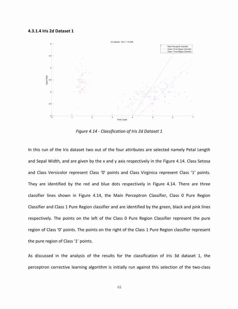
4.3.1.4 Iris 2d Dataset 1
Figure 4.14 - Classification of Iris 2d Dataset 1
In this run of the Iris dataset two out of the four attributes are selected namely Petal Length
and Sepal Width, and are given by the x and y axis respectively in the Figure 4.14. Class Setosa
and Class Versicolor represent Class ‘0’ points and Class Virginica represent Class ‘1’ points.
They are identified by the red and blue dots respectively in Figure 4.14. There are three
classifier lines shown in Figure 4.14, the Main Perceptron Classifier, Class 0 Pure Region
Classifier and Class 1 Pure Region classifier and are identified by the green, black and pink lines
respectively. The points on the left of the Class 0 Pure Region Classifier represent the pure
region of Class ‘0’ points. The points on the right of the Class 1 Pure Region classifier represent
the pure region of Class ‘1’ points.
As discussed in the analysis of the results for the classification of Iris 3d dataset 1, the
perceptron corrective learning algorithm is initially run against this selection of the two-class
0 1 2 3 4 5 6 72
2.5
3
3.5
4
4.5
5Iris Dataset - Run 1 - PLvSW
Petal Length
Sep
al W
idth
Main Perceptron ClassifierClass 0 Pure Region ClassifierClass 1 Pure Region Classifier
49
Iris dataset with a random initial weight vector until the best possible classification of the
dataset is reached. This classifier is determined to be the Main Perceptron Classifier (green line
in Figure 4.14) and the final weight vector of this line is used as the initial weight vector for
determining the pure regions of data which can be identified as the Class 0 Pure Region
Classifier and Class 1 Pure Region Classifier.
Main Perceptron Classifier
Class Left
Entropy
Class Right
Entropy
Total Weighted Entropy
Number of Epochs to
Classify
Total Time taken to Run Classifier
(in seconds)
w1 w2 w3
0.21 0.75 0.43 9 0.38 -3.15 4.84 0.64
Table 4.17 - Results of Main Perceptron Classifier on Iris 2d dataset 1
We can see from Table 4.17 that the classifier takes 9 epochs and 0.38s to obtain the best
possible classification of the dataset (Main Perceptron Classifier from Figure 4.14). The final
weight vector (wt) of the classifier is provided in Table 4.17 as w1, w2 and w3.
As discussed in the analysis of the results for the classification of Iris 3d dataset 1, we then run
an optimized version of the perceptron corrective learning algorithm with the starting weight
vector which was obtained from the previous run (w1, w2, w3 from Table 4.17). The algorithm
is run to find the pure region of Class ‘0’ points, we determine that we have found a pure region
of Class ‘0’ points for a ∆e value at which the Class Left Entropy reaches 0 and Purity of Class ‘0’
points reaches 1. This classifier is determined to be the Class 0 Pure Region Classifier (black line
in Figure 4.14).
As discussed in the analysis of the results for the classification of Iris 3d dataset 1, we then run

50
another optimized version of the perceptron corrective learning algorithm with the starting
weight vector which was obtained from the main Classifier (w1, w2, w3 from Table 4.17). The
algorithm is run to find the pure region of Class ‘1’ points, we determine that we have found a
pure region of Class ‘1’ points for a ∆e value at which the Class Right Entropy reaches 0 and
Purity of Class ‘1’ points reaches 1. This classifier is determined to be the Class 1 Pure Region
Classifier (pink line in Figure 4.14).
Figure 4.15 - Entropy & Purity versus ∆e for Class ‘0’ Pure Classifier on Iris 2d dataset 1
As discussed in the analysis of the results for the classification of Iris 3d dataset 1, we can see
from Figure 4.15 that the Class Left Entropy (orange curve) is gradually decreasing and the Class
Right Entropy (grey curve) is gradually increasing which is an indication that the purity of points
on the left side of the classifier is increasing.
0.00
0.20
0.40
0.60
0.80
1.00
0.02 0.05 0.10 0.15 0.20 0.25 0.30 0.35 0.40 0.45 0.46 0.47 0.48 0.49Relative Weight For Error Correction - Class 0Class Left Entropy Class Right Entropy
Total Weighted Entropy Purity of Class 0 Points

51
Table 4.18 - Results of Class ‘0’ Pure Classifier on Iris 2d dataset 1
We can also see from Figure 4.15 and Table 4.18 that when the Class Left Entropy reaches its
minimum value (0.0) at ∆e = 0.45, the purity of Class ‘0’ points is at its maximum value (1.0). We
have now obtained a pure region of Class ‘0’ points at this ∆e value.
Table 4.19 - Confusion Matrix and Accuracy of Class ‘0’ Pure Classifier on Iris 2d dataset 1
As discussed in the analysis of the results for the classification of Iris 3d dataset 1, Table 4.19
provides a tabulation of the count of the number of class instances correctly and incorrectly
PURE CLASS MIXED CLASS PRECISION 1.00
PURE CLASS 93 7 RECALL 0.93
MIXED CLASS 0 50 F-MEASURE 0.96
Predicted Class
Actual Class
Class 0 Pure Classifier
Class 1 Correction
Class Left
Entropy
Class Right
Entropy
Total Weighted Entropy
Purity of Class 0 Points
Number of Epochs to Classify
Total Time taken to Run Classifier
(in seconds)
0.02 0.68 0.45 0.63 0.82 500 14.03
0.05 0.47 0.28 0.42 0.90 500 13.14
0.10 0.32 0.26 0.30 0.94 500 14.00
0.15 0.24 0.33 0.27 0.96 500 13.60
0.20 0.14 0.45 0.25 0.98 500 13.35
0.25 0.14 0.45 0.25 0.98 500 14.07
0.30 0.15 0.50 0.27 0.98 500 13.75
0.35 0.15 0.50 0.27 0.98 500 12.86
0.40 0.15 0.50 0.27 0.98 500 13.42
0.45 0.00 0.58 0.22 1.00 298 8.40
0.46 0.00 0.58 0.22 1.00 288 8.20
0.47 0.00 0.58 0.22 1.00 279 7.75
0.48 0.00 0.58 0.22 1.00 270 7.56
0.49 0.00 0.58 0.22 1.00 262 7.44
52
predicted by the Class ‘0’ Pure Region Classifier and is known as a confusion matrix. Precision,
recall and F-measure values are also provided to highlight the accuracy of the classifier.
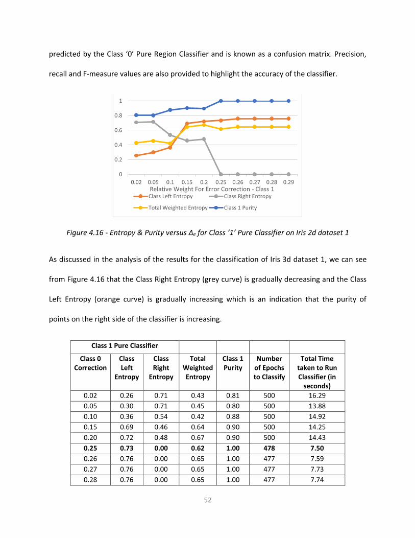
Figure 4.16 - Entropy & Purity versus ∆e for Class ‘1’ Pure Classifier on Iris 2d dataset 1
As discussed in the analysis of the results for the classification of Iris 3d dataset 1, we can see
from Figure 4.16 that the Class Right Entropy (grey curve) is gradually decreasing and the Class
Left Entropy (orange curve) is gradually increasing which is an indication that the purity of
points on the right side of the classifier is increasing.
Class 1 Pure Classifier
Class 0 Correction
Class Left
Entropy
Class Right
Entropy
Total Weighted Entropy
Class 1 Purity
Number of Epochs to Classify
Total Time taken to Run Classifier (in
seconds)
0.02 0.26 0.71 0.43 0.81 500 16.29
0.05 0.30 0.71 0.45 0.80 500 13.88
0.10 0.36 0.54 0.42 0.88 500 14.92
0.15 0.69 0.46 0.64 0.90 500 14.25
0.20 0.72 0.48 0.67 0.90 500 14.43
0.25 0.73 0.00 0.62 1.00 478 7.50
0.26 0.76 0.00 0.65 1.00 477 7.59
0.27 0.76 0.00 0.65 1.00 477 7.73
0.28 0.76 0.00 0.65 1.00 477 7.74
0
0.2
0.4
0.6
0.8
1
0.02 0.05 0.1 0.15 0.2 0.25 0.26 0.27 0.28 0.29Relative Weight For Error Correction - Class 1Class Left Entropy Class Right Entropy
Total Weighted Entropy Class 1 Purity

53
0.29 0.76 0.00 0.65 1.00 477 7.76
Table 4.20 - Results of Class ‘1’ Pure Classifier on Iris 2d dataset 1
We can also see from Figure 4.16 and Table 4.20 that when the Class Right Entropy reaches its
minimum value (0.0) at ∆e = 0.25, the purity of Class ‘1’ points is at its maximum value (1.0). We
have now obtained a pure region of Class ‘1’ points at this ∆e value.
Table 4.21 - Confusion Matrix and Accuracy of Class ‘1’ Pure Classifier on Iris 2d dataset 1
As discussed in the analysis of the results for the classification of Iris 3d dataset 1, Table 4.11
provides a tabulation of the count of the number of class instances correctly and incorrectly
predicted by the Class ‘1’ Pure Region Classifier and is known as a confusion matrix. Precision,
recall and F-measure values are also provided to highlight the accuracy of the classifier.
PURE CLASS MIXED CLASS PRECISION 1.00
PURE CLASS 22 28 RECALL 0.44
MIXED CLASS 0 100 F-MEASURE 0.61
Predicted Class
Actual Class

54
4.3.1.5 Iris 2d Dataset 2
Figure 4.17 - Classification of Iris 2d Dataset 2
In this run of the Iris dataset two out of the four attributes are selected namely Petal Width and
Petal Length, and are given by the x and y axis respectively in the Figure 4.17.
Table 4.22 - Results of Main Perceptron Classifier on Iris 2d dataset 2
We can see from Table 4.22 that the classifier takes 500 epochs and 23.25s to obtain the best
possible classifier (Main Perceptron Classifier from Figure 4.17).
0 0.5 1 1.5 2 2.5 31
2
3
4
5
6
7Iris Dataset - Run 2 - PWvPL
Petal Width
Pet
al L
engt
h
Main Perceptron ClassifierClass 0 Pure Region ClassifierClass 1 Pure Region Classifier
Main Perceptron Classifier
Class Left
Entropy
Class Right
Entropy
Total Weighted Entropy
Number of Epochs to
Classify
Total Time taken to Run Classifier
(in seconds)
0.08 0.54 0.26 500 23.25

55
Figure 4.18 - Entropy & Purity versus ∆e for Class ‘0’ Pure Classifier on Iris 2d dataset 2
As discussed in the analysis of the results for the classification of Iris 3d dataset 1, we can see
from Figure 4.18 that the Class Left Entropy (orange curve) is gradually decreasing and the Class
Right Entropy (grey curve) is gradually increasing which is an indication that the purity of points
on the left side of the classifier is increasing.
Table 4.23 - Results of Class ‘0’ Pure Classifier on Iris 2d dataset 2
0.00
0.20
0.40
0.60
0.80
1.00
0.02 0.05 0.10 0.15 0.20 0.25 0.26 0.27 0.28 0.29Relative Weight For Error Correction - Class 0Class Left Entropy Class Right Entropy
Total Weighted Entropy Class 0 Purity
Class 0 Pure Classifier
Class 1 Correction
Class Left
Entropy
Class Right
Entropy
Total Weighted Entropy
Class 0 Purity
Number of Epochs to Classify
Total Time taken to Run Classifier
(in seconds)
0.02 0.28 0.25 0.27 0.95 500 20.07
0.05 0.35 0.00 0.25 0.93 500 17.89
0.10 0.08 0.32 0.16 0.99 500 13.97
0.15 0.08 0.32 0.16 0.99 500 18.16
0.20 0.14 0.32 0.20 0.98 500 21.88
0.25 0.00 0.49 0.18 1.00 124 4.56
0.26 0.00 0.49 0.18 1.00 117 4.09
0.27 0.00 0.49 0.18 1.00 130 4.63
0.28 0.08 0.32 0.16 0.99 500 17.09
0.29 0.08 0.32 0.16 0.99 500 21.58

56
We can also see from Figure 4.18 and Table 4.23 that when the Class Left Entropy reaches its
minimum value (0.0) at ∆e = 0.25, the purity of Class ‘1’ points is at its maximum value (1.0). We
have now obtained a pure region of Class ‘1’ points at this ∆e value.
Table 4.24 - Confusion Matrix and Accuracy of Class ‘0’ Pure Classifier on Iris 2d dataset 2
As discussed in the analysis of the results for the classification of Iris 3d dataset 1, Table 4.24
provides a tabulation of the count of the number of class instances correctly and incorrectly
predicted by the Class ‘0’ Pure Region Classifier and is known as a confusion matrix. Precision,
recall and F-measure values are also provided to highlight the accuracy of the classifier.
Figure 4.19 - Entropy & Purity versus ∆e for Class ‘1’ Pure Classifier on Iris 2d dataset 2
As discussed in the analysis of the results for the classification of Iris 3d dataset 1, we can see
from Figure 4.19 that the Class Right Entropy (grey curve) is at the minimum value (0.0) which
indicates a pure region of points on the right side of the classifier.
PURE CLASS MIXED CLASS PRECISION 1.00
PURE CLASS 96 4 RECALL 0.96
MIXED CLASS 0 50 F-MEASURE 0.98
Predicted Class
Actual Class
0.00
0.20
0.40
0.60
0.80
1.00
0.02 0.03 0.04 0.05 0.06Relative Weight For Error Correction - Class 1
Class Left Entropy Class Right Entropy
Total Weighted Entropy Class 1 Purity
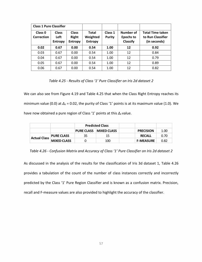
57
Class 1 Pure Classifier
Class 0 Correction
Class Left
Entropy
Class Right
Entropy
Total Weighted Entropy
Class 1 Purity
Number of Epochs to
Classify
Total Time taken to Run Classifier
(in seconds)
0.02 0.67 0.00 0.54 1.00 12 0.92
0.03 0.67 0.00 0.54 1.00 12 0.84
0.04 0.67 0.00 0.54 1.00 12 0.79
0.05 0.67 0.00 0.54 1.00 12 0.89
0.06 0.67 0.00 0.54 1.00 12 0.82
Table 4.25 - Results of Class ‘1’ Pure Classifier on Iris 2d dataset 2
We can also see from Figure 4.19 and Table 4.25 that when the Class Right Entropy reaches its
minimum value (0.0) at ∆e = 0.02, the purity of Class ‘1’ points is at its maximum value (1.0). We
have now obtained a pure region of Class ‘1’ points at this ∆e value.
Table 4.26 - Confusion Matrix and Accuracy of Class ‘1’ Pure Classifier on Iris 2d dataset 2
As discussed in the analysis of the results for the classification of Iris 3d dataset 1, Table 4.26
provides a tabulation of the count of the number of class instances correctly and incorrectly
predicted by the Class ‘1’ Pure Region Classifier and is known as a confusion matrix. Precision,
recall and F-measure values are also provided to highlight the accuracy of the classifier.
PURE CLASS MIXED CLASS PRECISION 1.00
PURE CLASS 35 15 RECALL 0.70
MIXED CLASS 0 100 F-MEASURE 0.82
Predicted Class
Actual Class
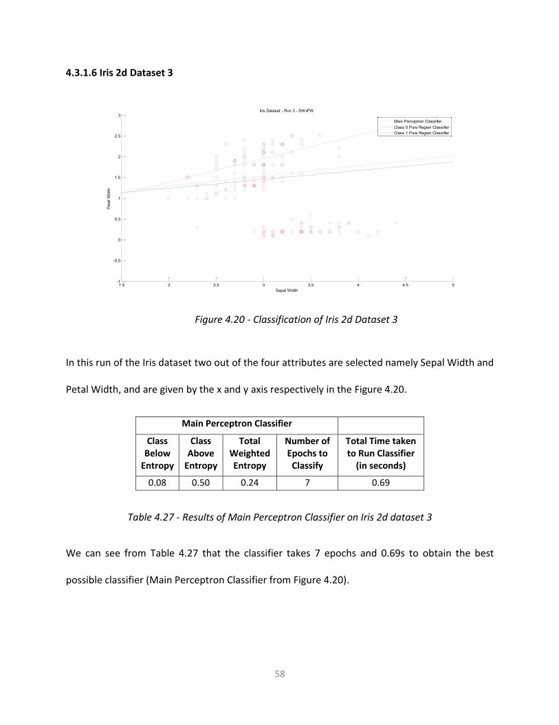
58
4.3.1.6 Iris 2d Dataset 3
Figure 4.20 - Classification of Iris 2d Dataset 3
In this run of the Iris dataset two out of the four attributes are selected namely Sepal Width and
Petal Width, and are given by the x and y axis respectively in the Figure 4.20.
Main Perceptron Classifier
Class Below
Entropy
Class Above
Entropy
Total Weighted Entropy
Number of Epochs to
Classify
Total Time taken to Run Classifier
(in seconds)
0.08 0.50 0.24 7 0.69
Table 4.27 - Results of Main Perceptron Classifier on Iris 2d dataset 3
We can see from Table 4.27 that the classifier takes 7 epochs and 0.69s to obtain the best
possible classifier (Main Perceptron Classifier from Figure 4.20).
1.5 2 2.5 3 3.5 4 4.5 5-1
-0.5
0
0.5
1
1.5
2
2.5
3Iris Dataset - Run 3 - SWvPW
Sepal Width
Pet
al W
idth
Main Perceptron ClassifierClass 0 Pure Region ClassifierClass 1 Pure Region Classifier

59
Figure 4.21 - Entropy & Purity versus ∆e for Class ‘0’ Pure Classifier on Iris 2d dataset 3
As discussed in the analysis of the results for the classification of Iris 3d dataset 1, we can see
from Figure 4.21 that the Class Left Entropy (orange curve) is gradually decreasing and the Class
Right Entropy (grey curve) is gradually increasing which is an indication that the purity of points
on the left side of the classifier is increasing.
Class 0 Pure Classifier
Class 1 Correction
Class Left
Entropy
Class Right
Entropy
Total Weighted Entropy
Class 0 Purity
Number of Epochs to Classify
Total Time taken to Run Classifier
(in seconds)
0.02 0.24 0.15 0.21 0.96 500 20.19
0.05 0.24 0.15 0.21 0.96 500 13.24
0.10 0.24 0.33 0.27 0.96 500 16.57
0.15 0.15 0.50 0.27 0.98 500 14.42
0.20 0.08 0.50 0.24 0.99 500 11.94
0.25 0.09 0.62 0.29 0.99 500 18.16
0.30 0.00 0.71 0.29 1.00 7 0.57
0.31 0.00 0.76 0.32 1.00 7 0.31
0.32 0.00 0.76 0.32 1.00 7 0.31
0.33 0.00 0.78 0.34 1.00 7 0.36
0.34 0.00 0.80 0.35 1.00 7 0.31
Table 4.28 - Results of Class ‘0’ Pure Classifier on Iris 2d dataset 3
0
0.2
0.4
0.6
0.8
1
0.02 0.05 0.1 0.15 0.2 0.25 0.3 0.31 0.32 0.33Relative Weight For Error Correction - Class 0
Class Left Entropy Class Right Entropy
Total Weighted Entropy Class 0 Purity

60
We can also see from Figure 4.21 and Table 4.28 that when the Class Left Entropy reaches its
minimum value (0.0) at ∆e = 0.30, the purity of Class ‘0’ points is at its maximum value (1.0). We
have now obtained a pure region of Class ‘0’ points at this ∆e value.
Table 4.29 - Confusion Matrix and Accuracy of Class ‘0’ Pure Classifier on Iris 2d dataset 3
As discussed in the analysis of the results for the classification of Iris 3d dataset 1, Table 4.29
provides a tabulation of the count of the number of class instances correctly and incorrectly
predicted by the Class ‘0’ Pure Region Classifier and is known as a confusion matrix. Precision,
recall and F-measure values are also provided to highlight the accuracy of the classifier.
Figure 4.22 - Entropy & Purity versus ∆e for Class ‘1’ Pure Classifier on Iris 2d dataset 3
As discussed in the analysis of the results for the classification of Iris 3d dataset 1, we can see
from Figure 4.22 that the Class Right Entropy (grey curve) is at the minimum value (0.0) which
indicates a pure region of points on the right side of the classifier.
PURE CLASS MIXED CLASS PRECISION 1.00
PURE CLASS 88 12 RECALL 0.88
MIXED CLASS 0 50 F-MEASURE 0.94
Predicted Class
Actual Class
0
0.2
0.4
0.6
0.8
1
0.02 0.03 0.04 0.05 0.06 0.07 0.08 0.09Relative Weight For Error Correction - Class 1
Class Left Entropy Class Right Entropy
Total Weighted Entropy Class 1 Purity

61
Class 1 Pure Classifier
Class 0 Correction
Class Left
Entropy
Class Right
Entropy
Total Weighted Entropy
Class 1 Purity
Number of Epochs to Classify
Total Time taken to Run Classifier
(in seconds)
0.02 0.63 0.00 0.50 1.00 345 14.04
0.03 0.63 0.00 0.50 1.00 366 12.63
0.04 0.62 0.00 0.48 1.00 378 14.28
0.05 0.60 0.00 0.47 1.00 392 13.01
0.06 0.60 0.00 0.47 1.00 405 13.57
0.07 0.60 0.00 0.47 1.00 420 14.51
0.08 0.60 0.00 0.47 1.00 435 13.08
0.09 0.60 0.00 0.47 1.00 454 44.43
Table 4.30 - Results of Class ‘1’ Pure Classifier on Iris 2d dataset 3
We can also see from Figure 4.22 and Table 4.30 that when the Class Right Entropy reaches its
minimum value (0.0) at ∆e = 0.02, the purity of Class ‘1’ points is at its maximum value (1.0). We
have now obtained a pure region of Class ‘1’ points at this ∆e value.
Table 4.31 - Confusion Matrix and Accuracy of Class ‘1’ Pure Classifier on Iris 2d dataset 3
As discussed in the analysis of the results for the classification of Iris 3d dataset 1, Table 4.31
provides a tabulation of the count of the number of class instances correctly and incorrectly
predicted by the Class ‘1’ Pure Region Classifier and is known as a confusion matrix. Precision,
recall and F-measure values are also provided to highlight the accuracy of the classifier.
PURE CLASS MIXED CLASS PRECISION 1.00
PURE CLASS 29 21 RECALL 0.58
MIXED CLASS 0 100 F-MEASURE 0.73Actual Class
Predicted Class

62
4.3.1.7 Test 2d Dataset 1
Figure 4.23 - Classification of Test 2d Dataset 1
This 2d dataset was created with ninety seven instances. These contain both Class ‘1’ and Class
‘0’ points and could be separated into four distinct regions as can be seen in Figure 4.23. The x
axis refers to abscissa of the point and y axis refers to the ordinate of the point. Class ‘0’ and
Class ‘1’ points can be identified by the red and blue dots respectively in Figure 4.23. There are
three line classifiers shown in Figure 4.23, the Main Perceptron Classifier, Class 0 Pure Region
Classifier and Class 1 Pure Region classifier and are identified by the green, black and pink lines
respectively. The points below the Class 0 Pure Region Classifier represent the pure region of
Class ‘0’ points. The points on the left of the Class 1 Pure Region classifier represent the pure
region of Class ‘1’ points.
As discussed in the analysis of the results for the classification of Iris 3d dataset 1, the
perceptron corrective learning algorithm is initially run against this two-class dataset with a
-4 -3 -2 -1 0 1 2 3 4 5-1
-0.5
0
0.5
1
1.5
2
2.5
3
3.5
4Test Dataset - Run 1 - 4 Distinct Regions
X
Y
Main Perceptron ClassifierClass 0 Pure Region ClassifierClass 1 Pure Region Classifier

63
random initial weight vector until the best possible classification is reached. This classifier is
determined to be the Main Perceptron Classifier (green line in Figure 4.23) and the final weight
vector of this line is used as the initial weight vector for determining the pure regions of data
which can be identified as the Class 0 Pure Region Classifier and Class 1 Pure Region Classifier.
Main Perceptron Classifier
Class Left
Entropy
Class Right
Entropy
Total Weighted Entropy
Number of Epochs to
Classify
Total Time taken to Run Classifier
(in seconds)
w1 w2 w3
0.89 0.52 0.79 47 0.88 -0.03 0.00 0.00
Table 4.32 - Results of Main Perceptron Classifier on Test 2d dataset 1
We can see from Table 4.32 that the classifier takes 47 epochs and 0.88s to obtain the best
possible classification of the dataset (Main Perceptron Classifier from Figure 4.23). The final
weight vector (wt) of the classifier is provided in Table 4.20 as w1, w2 and w3.
As discussed in the analysis of the results for the classification of Iris 3d dataset 1, we then run
an optimized version of the perceptron corrective learning algorithm with the starting weight
vector which was obtained from the previous run (w1, w2, w3 from Table 4.32). The algorithm
is run to find the first pure region of Class ‘0’ points, we determine that we have found a pure
region of Class ‘0’ points for a ∆e value at which the Class Left Entropy reaches 0 and Purity of
Class ‘0’ points reaches 1. This classifier is determined to be the First Class 0 Pure Region
Classifier (black line in Figure 4.23).
As discussed in the analysis of the results for the classification of Iris 3d dataset 1, we then run

64
another optimized version of the perceptron corrective learning algorithm with the starting
weight vector which was obtained from the main perceptron classifier (w1, w2, w3 from Table
4.32). The algorithm is run to find the first pure region of Class ‘1’ points, we determine that we
have found a pure region of Class ‘1’ points for a ∆e value at which the Class Right Entropy
reaches 0 and Purity of Class ‘1’ points reaches 1. This classifier is determined to be the Class 1
Pure Region Classifier (pink line in Figure 4.23).
Figure 4.24 - Entropy & Purity versus ∆e for Class ‘0’ Pure Classifier on Test 2d dataset 1
As discussed in the analysis of the results for the classification of Iris 3d dataset 1, we can see
from Figure 4.24 that the Class Left Entropy (orange curve) is at the minimum value (0.0) which
indicates a pure region of points on the left side of the classifier.
Class 0 Pure Classifier
Class 1 Correction
Class Left
Entropy
Class Right
Entropy
Total Weighted Entropy
Class 0 Purity
Number of Epochs to Classify
Total Time taken to Run Classifier
(in seconds)
0.01 0.00 1.00 0.86 1.00 7 0.14
0.02 0.00 0.99 0.84 1.00 7 0.13
0.03 0.96 1.00 0.98 0.61 500 6.45
0.04 0.00 0.99 0.83 1.00 21 0.25
0.00
0.20
0.40
0.60
0.80
1.00
0.01 0.02 0.03 0.04 0.05Relative Weight For Error Correction - Class 1
Class Left Entropy Class Right Entropy
Total Weighted Entropy Class 0 Purity

65
0.05 0.00 0.99 0.84 1.00 16 0.23
Table 4.33 - Results of Class ‘0’ Pure Classifier on Test 2d dataset 1
We can also see from Figure 4.24 and Table 4.33 that when the Class Left Entropy reaches its
minimum value (0.0) at ∆e = 0.01, the purity of Class ‘1’ points is at its maximum value (1.0). We
have now obtained a pure region of Class ‘0’ points at this ∆e value.
Table 4.34 - Confusion Matrix and Accuracy of Class ‘0’ Pure Classifier on Test 2d dataset 1
As discussed in the analysis of the results for the classification of Iris 3d dataset 1, Table 4.34
provides a tabulation of the count of the number of class instances correctly and incorrectly
predicted by the Class ‘0’ Pure Region Classifier and is known as a confusion matrix. Precision,
recall and F-measure values are also provided to highlight the accuracy of the classifier.
Figure 4.25 - Entropy & Purity versus ∆e for Class ‘1’ Pure Classifier on Test 2d dataset 1
PURE CLASS MIXED CLASS PRECISION 1.00
PURE CLASS 16 7 RECALL 0.70
MIXED CLASS 0 74 F-MEASURE 0.82
Predicted Class
Actual Class
0.00
0.20
0.40
0.60
0.80
1.00
0.02 0.05 0.10 0.11 0.12 0.13 0.14Relative Weight For Error Correction - Class 0
Class Left Entropy Class Right Entropy
Total Weighted Entropy Class 1 Purity
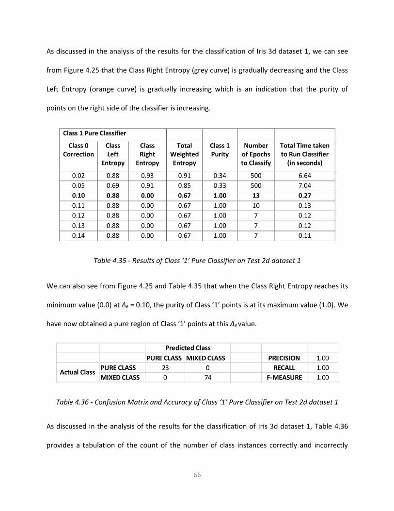
66
As discussed in the analysis of the results for the classification of Iris 3d dataset 1, we can see
from Figure 4.25 that the Class Right Entropy (grey curve) is gradually decreasing and the Class
Left Entropy (orange curve) is gradually increasing which is an indication that the purity of
points on the right side of the classifier is increasing.
Class 1 Pure Classifier
Class 0 Correction
Class Left
Entropy
Class Right
Entropy
Total Weighted Entropy
Class 1 Purity
Number of Epochs to Classify
Total Time taken to Run Classifier
(in seconds)
0.02 0.88 0.93 0.91 0.34 500 6.64
0.05 0.69 0.91 0.85 0.33 500 7.04
0.10 0.88 0.00 0.67 1.00 13 0.27
0.11 0.88 0.00 0.67 1.00 10 0.13
0.12 0.88 0.00 0.67 1.00 7 0.12
0.13 0.88 0.00 0.67 1.00 7 0.12
0.14 0.88 0.00 0.67 1.00 7 0.11
Table 4.35 - Results of Class ‘1’ Pure Classifier on Test 2d dataset 1
We can also see from Figure 4.25 and Table 4.35 that when the Class Right Entropy reaches its
minimum value (0.0) at ∆e = 0.10, the purity of Class ‘1’ points is at its maximum value (1.0). We
have now obtained a pure region of Class ‘1’ points at this ∆e value.
Table 4.36 - Confusion Matrix and Accuracy of Class ‘1’ Pure Classifier on Test 2d dataset 1
As discussed in the analysis of the results for the classification of Iris 3d dataset 1, Table 4.36
provides a tabulation of the count of the number of class instances correctly and incorrectly
PURE CLASS MIXED CLASS PRECISION 1.00
PURE CLASS 23 0 RECALL 1.00
MIXED CLASS 0 74 F-MEASURE 1.00
Predicted Class
Actual Class

67
predicted by the Class ‘1’ Pure Region Classifier and is known as a confusion matrix. Precision,
recall and F-measure values are also provided to highlight the accuracy of the classifier.
Figure 4.26 - Class ’0’ Pure Region Removed From Test 2d Dataset 1
Figure 4.27 - Class ’1’ Pure Region Removed From Test 2d Dataset 1
As discussed in Chapter 3, In order to determine the remaining pure regions of data, we now
remove the identified pure region of Class ‘0’ and Class ‘1’ points from our dataset. Figure 4.26
and 4.27 show the dataset with the pure region of Class ‘0’ points and pure region of Class ‘1’
points removed respectively.
-4 -3 -2 -1 0 1 2 3 4 5-1
-0.5
0
0.5
1
1.5
2
2.5
3
3.5
4
-4 -3 -2 -1 0 1 2 3 4 5-1
-0.5
0
0.5
1
1.5
2
2.5
3
3.5
4
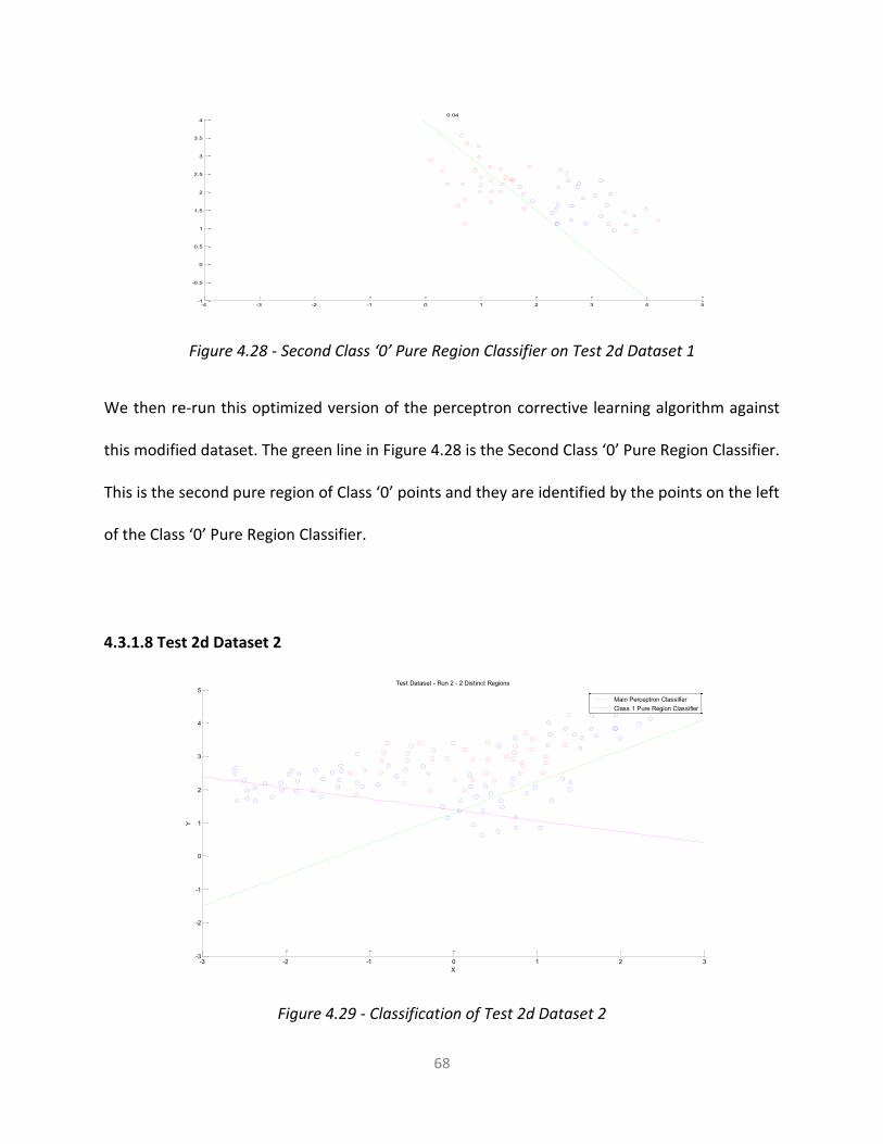
68
Figure 4.28 - Second Class ‘0’ Pure Region Classifier on Test 2d Dataset 1
We then re-run this optimized version of the perceptron corrective learning algorithm against
this modified dataset. The green line in Figure 4.28 is the Second Class ‘0’ Pure Region Classifier.
This is the second pure region of Class ‘0’ points and they are identified by the points on the left
of the Class ‘0’ Pure Region Classifier.
4.3.1.8 Test 2d Dataset 2
Figure 4.29 - Classification of Test 2d Dataset 2
-4 -3 -2 -1 0 1 2 3 4 5-1
-0.5
0
0.5
1
1.5
2
2.5
3
3.5
40.04
-3 -2 -1 0 1 2 3-3
-2
-1
0
1
2
3
4
5Test Dataset - Run 2 - 2 Distinct Regions
X
Y
Main Perceptron ClassifierClass 1 Pure Region Classifier

69
This 2d dataset was created with one hundred and twenty three instances. These contain both
Class ‘1’ and Class ‘0’ points as can be seen in Figure 4.29. The x axis refers to abscissa of the
point and y axis refers to the ordinate of the point. Class ‘0’ and Class ‘1’ points can be
identified by the red and blue dots respectively in Figure 4.29. There are two line classifiers
shown in Figure 4.29, the Main Perceptron Classifier and Class 1 Pure Region classifier and are
identified by the green and pink lines respectively. The points below the Class 1 Pure Region
Classifier in Figure 4.29 represent the pure region of Class ‘1’ points. We are unable to
determine a pure region of Class ‘0’ points in this dataset.
As discussed in the analysis of the results for the classification of Iris 3d dataset 1, the
perceptron corrective learning algorithm is initially run against this two-class dataset with a
random initial weight vector until the best possible classification is reached. This classifier is
determined to be the Main Perceptron Classifier (green line in Figure 4.29) and the final weight
vector of this line is used as the initial weight vector for determining the pure region of data
which can be identified as the Class 1 Pure Region Classifier.
Main Perceptron Classifier
Class Left
Entropy
Class Right
Entropy
Total Weighted Entropy
Number of Epochs to Classify
Total Time taken to Run Classifier
(in seconds)
w1 w2 w3
0.00 0.98 0.85 500 6.09 0.23 -0.25 0.33
Table 4.37 - Results of Main Perceptron Classifier on Test 2d dataset 2
We can see from Table 4.37 that the classifier takes 500 epochs and 6.09s to obtain the best
possible classifier (Main Perceptron Classifier from Figure 4.29). The final weight vector (wt) of
the classifier is provided in Table 4.37 as w1, w2 and w3.

70
Figure 4.30 - Entropy & Purity versus ∆e for Class ‘0’ Pure Classifier on Test 2d dataset 2
We can see from Figure 4.30 that the Class Left Entropy (orange line, which is hidden behind
the total weighted entropy (yellow line)) does not reach the minimum value (0.0) which
indicates we are unable to obtain a pure region of Class ‘0’ points on either side of the classifier.
Class 0 Pure Classifier
Class 1 Correction
Class Left
Entropy
Class Right
Entropy
Total Weighted Entropy
Class 0 Purity
Number of Epochs to
Classify
Total Time taken to Run Classifier
(in seconds)
0.01 0.95 0.00 0.95 0.37 13 0.23
0.02 0.95 0.00 0.95 0.37 7 0.09
0.03 0.95 0.00 0.95 0.37 7 0.09
0.04 0.95 0.00 0.95 0.37 7 0.14
0.05 0.95 0.00 0.94 0.37 7 0.10
Table 4.38 - Results of Class ‘0’ Pure Classifier on Test 2d dataset 2
We can also see from Figure 4.30 and Table 4.38 that the Class Left Entropy and the purity of
Class ‘0’ points does not reach their minimum value (0.0) and maximum value (1.0)
respectively. We are unable to obtain a pure region of Class ‘0’ points for this dataset.
0.00
0.20
0.40
0.60
0.80
1.00
0.01 0.02 0.03 0.04 0.05Relative Weight For Error Correction - Class 1Class Left Entropy Class Right Entropy
Total Weighted Entropy Class 0 Purity

71
Table 4.39 - Confusion Matrix and Accuracy of Class ‘0’ Pure Classifier on Test 2d dataset 2
As discussed in the analysis of the results for the classification of Iris 3d dataset 1, Table 4.39
provides a tabulation of the count of the number of class instances correctly and incorrectly
predicted by the Class ‘0’ Pure Region Classifier and is known as a confusion matrix. Precision,
recall and F-measure values are also provided to highlight the accuracy of the classifier. Since
we are unable to obtain a pure region of Class ‘0’ points for this dataset, we can also see from
Table 4.39 that the precision of this classifier has a very low value (0.37).
Figure 4.31 - Entropy & Purity versus ∆e for Class ‘1’ Pure Classifier on Test 2d dataset 2
As discussed in the analysis of the results for the classification of Iris 3d dataset 1, we can see
from Figure 4.31 that the Class Right Entropy (grey curve) is at the minimum value (0.0) which
indicates a pure region of points on the right side of the classifier.
PURE CLASS MIXED CLASS PRECISION 0.37
PURE CLASS 45 0 RECALL 1.00
MIXED CLASS 78 0 F-MEASURE 0.54
Predicted Class
Actual Class
0.00
0.20
0.40
0.60
0.80
1.00
1.00 1.00 1.00 1.00 1.00Relative Weight For Error Correction - Class 0Class Left Entropy Class Right Entropy
Total Weighted Entropy Class 1 Purity

72
Table 4.40 - Results of Class ‘1’ Pure Classifier on Test 2d dataset 2
We can also see from Figure 4.31 and Table 4.40 that when the Class Right Entropy reaches its
minimum value (0.0) at ∆e = 0.01, the purity of Class ‘1’ points is at its maximum value (1.0). We
have now obtained a pure region of Class ‘1’ points at this ∆e value.
Table 4.41 - Confusion Matrix and Accuracy of Class ‘1’ Pure Classifier on Test 2d dataset 2
As discussed in the analysis of the results for the classification of Iris 3d dataset 1, Table 4.41
provides a tabulation of the count of the number of class instances correctly and incorrectly
predicted by the Class ‘1’ Pure Region Classifier and is known as a confusion matrix. Precision,
recall and F-measure values are also provided to highlight the accuracy of the classifier.
PURE CLASS MIXED CLASS PRECISION 1.00
PURE CLASS 16 50 RECALL 0.24
MIXED CLASS 0 67 F-MEASURE 0.39
Predicted Class
Actual Class
Class 1 Pure Classifier
Class 0 Correction
Class Left
Entropy
Class Right
Entropy
Total Weighted Entropy
Class 1 Purity
Number of Epochs to Classify
Total Time taken to Run Classifier
(in seconds)
0.01 0.96 0.00 0.91 1.00 500 4.60
0.02 0.98 0.00 0.85 1.00 500 4.48
0.03 0.99 0.23 0.83 0.96 500 4.44
0.04 1.00 0.52 0.83 0.88 500 4.47
0.05 1.00 0.69 0.85 0.82 500 4.47
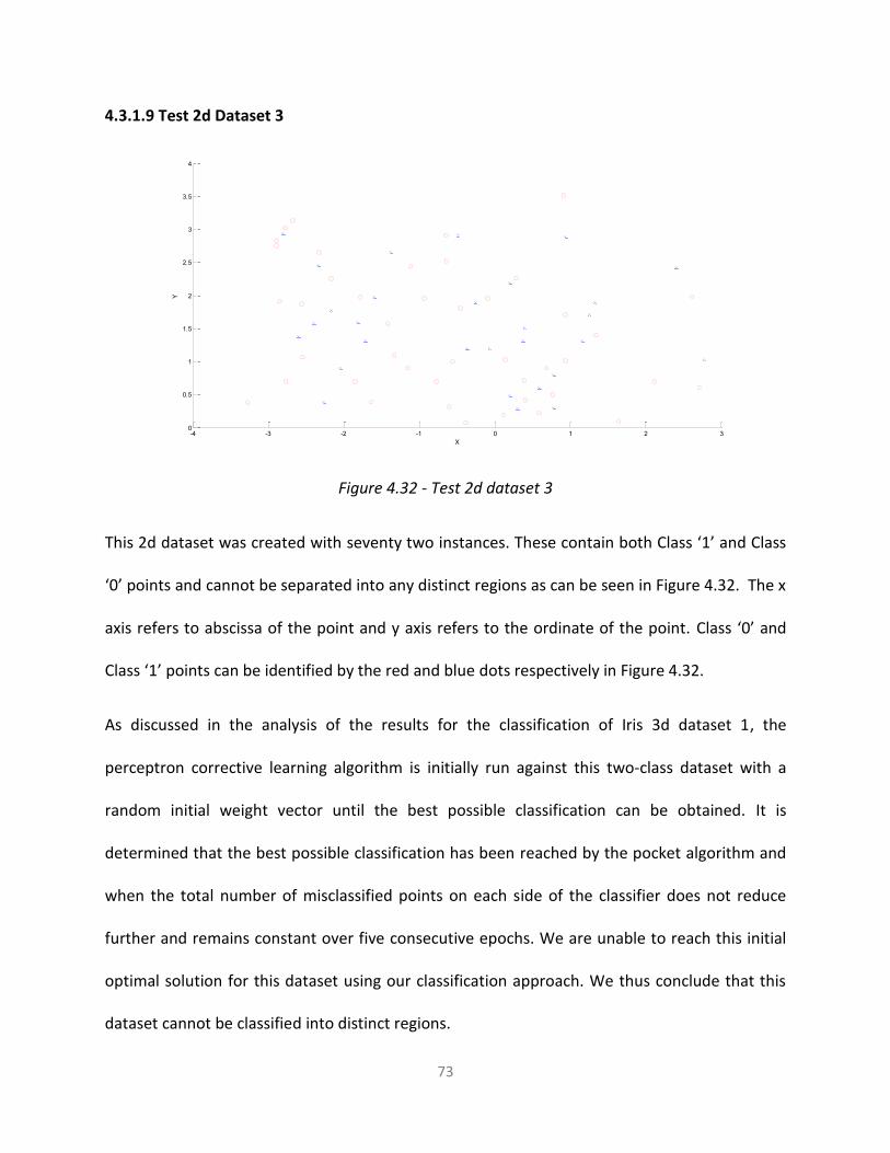
73
4.3.1.9 Test 2d Dataset 3
Figure 4.32 - Test 2d dataset 3
This 2d dataset was created with seventy two instances. These contain both Class ‘1’ and Class
‘0’ points and cannot be separated into any distinct regions as can be seen in Figure 4.32. The x
axis refers to abscissa of the point and y axis refers to the ordinate of the point. Class ‘0’ and
Class ‘1’ points can be identified by the red and blue dots respectively in Figure 4.32.
As discussed in the analysis of the results for the classification of Iris 3d dataset 1, the
perceptron corrective learning algorithm is initially run against this two-class dataset with a
random initial weight vector until the best possible classification can be obtained. It is
determined that the best possible classification has been reached by the pocket algorithm and
when the total number of misclassified points on each side of the classifier does not reduce
further and remains constant over five consecutive epochs. We are unable to reach this initial
optimal solution for this dataset using our classification approach. We thus conclude that this
dataset cannot be classified into distinct regions.
-4 -3 -2 -1 0 1 2 30
0.5
1
1.5
2
2.5
3
3.5
4
X
Y
74
Chapter 5
Conclusion and Future Work
In this section we provide a brief summary of the work implemented in this thesis and also
discuss a few improvements that can be made to our algorithm as part of the future work.
5.1 Conclusion
Classification algorithms have been used extensively over the past few decades. As discussed in
chapter 1 and 2 existing classifiers are able to accurately classify data but have some limitations
and drawbacks when it comes to identifying uniform regions from mixed regions of data in
selected datasets. SVM uses the concept of the high dimensional feature space to classify data
and the dimensionality of the feature space could become very large in size and be difficult to
be accommodated. The back propagation training algorithm when used on certain datasets
requires additional overhead such as many training runs to be able to accurately classify data.
In our research we have addressed these limitations in identification of uniform regions on
these datasets.

75
We discuss our algorithm and its design methodology in detail in chapter 3, It uses a supervised
learning with error correction approach to initially identify the best possible classification of the
dataset, which is said to have been obtained after the number of misclassified points does not
reduce any further and remains constant over five consecutive epochs. Once this initial
classifier is obtained, we then identify the distinct pure regions of Class ‘0’ and Class ‘1’ within
the dataset by utilizing the relative weight factor (∆e) while updating the weight vector for
misclassified Class ‘1’ and Class ‘0’ instance respectively. We are able to successfully identify
pure regions of data using this classification approach.
Our algorithm was tested against eight different two-class datasets and is able to accurately
identify the pure regions of points with 100% precision when these pure regions exist within
the selected dataset. In chapter 4, we have provided our detailed analysis of the results and
have also highlighted the accuracy and the performance of our classifier. We have overcome
most of the limitations exhibited by the existing classifiers on various datasets using our
classification approach.
5.2 Future Work
There are couple of modifications that could be made as advances to the proposed algorithm.
The proposed classification approach has only been implemented for two-class datasets. The
algorithm could be modified to be able to accurately classify multi-class datasets. We also
require an additional step of pre-processing when identifying pure regions in the scenario when
the dataset has more than two distinct pure regions. The algorithm could increase its speed and

76
have better performance in removing this additional step of pre-processing when it is needed
to identify multiple distinct region of pure points from the data.
77
References
[1] a S. Introduction, “Neural Networks,” Neural Networks, vol. 7, no. 1, p. 509, 1996.
[2] M. Chakravarty and G. Keller, “An Introduction to Computing: With Haskell,” 2002.
[3] B. E. Boser, I. M. Guyon, and V. N. Vapnik, “A Training Algorithm for Optimal Margin
Classifiers,” Proc. 5th Annu. ACM Work. Comput. Learn. Theory, pp. 144–152, 1992.
[4] C. Cortes and V. Vapnik, “Support-vector networks,” Mach. Learn., vol. 20, no. 3, pp.
273–297, 1995.
[5] S. a N. Diego, “862 18 120,” no. V, 1985.
[6] S. I. Gallant, “Perceptron-Based Learning Algorithms,” vol. I, no. 2, 1990.
[7] “M. Lichman,” “{UCI} Machine Learning Repository,” 2013. [Online]. Available:
http://archive.ics.uci.edu/ml.
[8] M. Lichman, “{UCI} Machine Learning Repository - Iris Data,” 2013. [Online]. Available:
https://archive.ics.uci.edu/ml/machine-learning-databases/iris/iris.names .
[9] A. Edgar and F. Ronald, “Scatter Plot of Iris Data,” 2007. [Online]. Available:
http://commons.wikimedia.org/wiki/File:Anderson%27s_Iris_data_set.png#globalusage.


![Recognition using Regions (Demo) Sudheendra V. Outline Generating multiple segmentations –Normalized cuts [Ren & Malik (2003)] Uniform regions –Watershed.](https://static.fdocuments.in/doc/165x107/56649e935503460f94b98a42/recognition-using-regions-demo-sudheendra-v-outline-generating-multiple.jpg)