IDENTIFICATION OF TOWER AND BOOM- WAKES USING … · Identification of Tower and Boom-Wakes Using...

http://www.iaeme.com/IJMET/index.asp 72 [email protected]

International Journal of Mechanical Engineering and Technology (IJMET)

Volume 10, Issue 06, June 2019, pp. 72-94. Article ID: IJMET_10_06_005

Available online at http://www.iaeme.com/ijmet/issues.asp?JType=IJMET&VType=10&IType=6

ISSN Print: 0976-6340 and ISSN Online: 0976-6359

© IAEME Publication

IDENTIFICATION OF TOWER AND BOOM-

WAKES USING COLLOCATED

ANEMOMETERS AND LIDAR MEASUREMENT

Maduako E. Okorie

Namibia University of Science and Technology, Private Bag 3388, Windhoek 9000, Namibia

Freddie Inambao

University of KwaZulu-Natal Durban 4041, South Africa

ABSTRACT

In this study the extent of tower and boom wake distortions were evaluated using

collocated anemometers and Lidar measurement based on wind data from Amperbo,

Namibia, where an existing latticed equilateral triangular communication tower was

instrumented according to IEC specifications. Wind data analysed was 10-minute

averaged, captured over a period of nine months (May to Sept. 2014). To enable further

and independent investigation of flow modification within the vicinity of the tower,

ZephIR 300 wind Lidar was installed at about 5.4 m from the foot of the tower. Wind

data from pairs of collocated cup anemometers located at 16.88 m and 64.97 m above

ground level (AGL) were analysed and compared to identify the range of directions that

were affected by the waking of the entire tower physical structure. Mean speed and

turbulence intensity (TI) were used in quantify the wake impact on the wind data

observed using cup anemometers, showing a speed deficit of up to 49 % and order of

magnitude increase in the TI for all the regions within the wake of the tower.

Comparison with ZephIR 300 observed mean speed resulted in a speed deficit of up to

50 % which further confirmed the extent of tower distortion and wake boundaries. The

Lidar also confirmed the speed-up effects and the asymmetric nature of the wake

boundaries associated with the mounting booms. The results show that TI analysis has

the potential to more accurately define the wake boundaries and wake distortion than

traditional speed ratios analysis. The study shows that the severity of tower wake effects

varies seasonally with winter months (June and July) recording the highest speed deficit

when compared to December, a summer month. Root Mean Square Errors (RMSE) were

further computed to ascertain the similarity degree of resource parameters from the two

measurement techniques, resulting in peak values of RMSE in the wake affected regions.

The TI approach consistently predicted larger wake boundaries than speed ratio

analysis. Wind direction analysis clearly showed the 180° ambiguity of ZephIR 300 and

the extent of deflection of the winds around the tower structure. Preliminary evaluation

of wake impact on the resource parameter shows that removing the sectors affected by

tower wakes leads to an increase in mean wind speed and a decrease in TI values.

Identification of Tower and Boom-Wakes Using Collocated Anemometers and Lidar

Measurement


Keywords: Tower wake, flow distortion, speed ratios, wind speed, speed deficit.

Cite this Article: Maduako E. Okorie and Freddie Inambao, Identification of Tower

and Boom-Wakes Using Collocated Anemometers and Lidar Measurement,

International Journal of Mechanical Engineering and Technology, 10(6), 2019, pp. 72-

94.

http://www.iaeme.com/IJMET/issues.asp?JType=IJMET&VType=10&IType=6

1. INTRODUCTION

Wind data for wind resource assessment in Namibia has been collected over the years by The

National Wind Recourse Assessment Project (NWRAP). Cost reduction and urgent

commencement of the project necessitated the use of existing communication towers for the

experiment. Towers belonging to Mobile Telecommunication Limited (MTC) were utilized.

The lattice equilateral triangular communication towers with boom-mounted anemometers

attached it were instrumented according to the IEC61400-12-1:2005(E) standard. Traditional

wind speed and directional measurement utilizes latticed or tubular towers with boom-mounted

anemometers attached to them. The best option [1], [2] would have been to mount the

anemometers on top of the tower to avoid any local wind flow modification by the tower

structure. This may not be a perfect option either because knowledge of the site shear trend is

needed to reduce project risk; as a result, booms are often placed below the tower top. The

obvious implication is that such an arrangement will inevitably expose the anemometer to the

flow distortion influence of the tower structure. Since the local wind flow at any site is not

constrained to a direction, the sensor at one time or the other might be directly in the tower’s

wake. Speed and direction sensors used at Amperbo, Namibia, are located below the top of the

tower. According to [3]– [6], arrangement of this sort exposes the speed sensors to tower

shadow effects. The tower induced flow modification, according to literature, contributes non-

negligible uncertainty on the wind data observed. This level of error is not acceptable in the

wind energy industry, where accuracy in wind measurement is needed for investment decision

making and project risk analysis. Previous works on tower shadow effect have found a 35 % to

50 % wind speed reduction and the severity is known to be directly related to different

configurations of the tower structure [7]– [10]. Such observations have been supported by

computational fluid dynamic approaches (CFD) [2], [6], [11]. According to [1], [2], for a

triangular lattice mast with thrust coefficient ( TC ) of 0.5, and 99.5 % centreline wind speed

deficit, dR is 5.7 times the width (Lm) of the tower phase. However, application of these studies

to towers of different structural configurations and possible different site atmospheric

conditions in the boundary layers are limited. The MTC tower at Amperbo has a unique

geometry and boom arrangement with numerous secondary support structures such as cross and

horizontal bracings, cable ladders, cable bundles and attachment brackets, which may

contribute to making flow around and through the tower more complex; a situation that

necessitates further investigation of the tower under consideration. To further identify the

boundaries of tower and boom wakes on the wind speed observed by the cup anemometer, an

additional independent instrument was used, namely, a continuous wave (CW) ground-based

profiling Lidar (Light Detection and Ranging) located about 5.4 m away from the foot of the

tower. This study utilized different approaches and various methodologies to identify the extent

of the tower and boom-wake distortion on the wind data measured with collocated anemometers

and the Lidar, by: (1) performing regression analysis, (2) comparing the speed ratios (3)

evaluating the Root Mean Square Errors (4), evaluating the tower distortion and scatter factors

and (5) analysis of wind direction differences for the concurrently observed wind data.

Maduako E. Okorie and Freddie Inambao


2. BACKGROUND

2.1. Site Description and Experimentation

Amperbo is a settlement in the Hardap region in Namibia, situated at 1152 m above sea level

(ASL). It is located at latitude 18.313°E and longitude 25.354°S. The test site is flat, and the

orography is gentle which qualifies the site as class A terrain according to Annex B of [2]. The

communication tower used belongs to the Mobile Communication Company (MTC) of

Namibia, the construction details of which are discussed in subsection 2.2 below. A QinetiQ

Ltd (UK) ZephIR Z300 Lidar (Light Detection and Ranging) provided by Masdar Institute of

Technology Abudabi, United Arab Emirates (UAE) was installed close to the foot of the tower.

Concerns on vandalism and damage from wild animals justified the placement of the Lidar in

a fenced area, although this raised the concern that the Lidar emitted laser might intersect the

guy wires at some heights. It is a homodyne continuous wave (CW) Doppler wind Lidar system

with 10 user programmable heights (besides a pre-fixed height of 38 m) up to 200 m, though

300 m can be selected, with a minimum measurement height of 10 m. The probe length is

designed to increase quadratically with height. At 10 m, the probe length is 0.07 m, whereas at

200 m, it is 30 m. The technical specification of the equipment indicates wind speed and wind

direction accuracies as < 0.1 m/s and < 0.5°, respectively [12–16]. It is a monostatic coaxial

system where emitted and backscattered light share common optics [17]. As a result of the

monostatic nature of ZephIR 300 and homodyne detection, meaning that only the absolute value

of the Doppler-shift is measured, there is 180° ambiguity in the measured wind direction [16].

To resolve this issue and provide an estimate of the site wind direction, ZephIR 300 has an

inbuilt meteorological station which measures other resource parameters, including wind

direction [14]. Each rotation of Lidar at every height takes 1 s, in which 50 measurements of

20 ms are taken, from which the 3D (i.e. horizontal and vertical wind speed, horizontal wind

direction) are generated. Lidar is specifically designed for autonomous wind assessment

campaign purposes where wind speed is measured by doppler shift effect. Z300 emits laser

radiation in a circular pattern by reflecting the laser beam off a spinning optical wedge, via the

Velocity Azimuth Display (VAD) scanning technique. The emitted laser beam hits the aerosol

in the atmosphere and scatters in-elastically. The detector records information about the return

signal by a coherent detection method and creates an electric signal that is digitally sampled for

determining the Doppler shifted frequency of the return light by comparing it to the transmitted

laser. The Doppler shifted frequency gives an idea of the wind speeds carrying the aerosols

[14], [17]

2.2. Tower Construction Detail and Instrumentation

The 120 m high guyed tower has an equilateral triangular cross-section with three vertical

tubular mild steel rods connected with a network of small angular cross bracings made from 45

mm x 45 mm x 5 mm angle bars. The leg distance or sides are 1.1 m throughout the height and

the vertical tubular rod each have a diameter of 100 mm. The boom has an outside diameter of

50 mm and wall thickness of 2 mm. The boom protrudes 2.56 m from the tower. Each discrete

member of the lattice tower generates a discrete wake which modifies local wind flow through

and around the tower structure (Figure 2a). Figure 2b is the top view of the boom arrangement

on the tower for the collocated speed sensors at 16.88 m and 64.92 m. Lm is leg distance or

phase width of the tower, Rd is the distance from the center of the communication tower, the

point of wind data observation, whereas a is the minimum boom length. The thrust coefficient

( TC ) of the tower is approximately 0.4495. The thrust coefficient may vary slightly depending

on the exact section of the tower considered. This was verified (Figure 2d) by a preliminary

computational fluid dynamic (CFD) study on the most convenient plane for positioning the


Measurement


anemometer in the tower to ensure minimum flow distortion. For the TC of approximately 0.45

and 99 % centerline wind speed deficit, dR is 3.74 times the width (Lm) of the tower phase.

Other secondary support structures such as ladder, cable bundles and attachment brackets were

not considered in estimating TC .This agrees with [2]. For a triangular lattice mast with thrust

coefficient ( TC ) of 0.5 and 99 % centerline wind speed deficit, dR is 3.7 times the leg length of

the tower.

a b

Figure 1. (a). Photograph of the MTC tower at Amperbo, looking up at the north facing side. The WS4

boom, WS4B boom and boom mounting of the wind vane are pictured extending out at 16.88 m

(AGL). The faces housing the climbing ladder and the cable bundles are shown. (b) The plan view

schematic of the tower showing the layout of the WS4 and WS4B booms shown at about 159° and 278°

respectively

c d

Figure 1. (c) The plan view schematics of the tower showing the configurations of the speed sensor

booms and associated dimensions. (d) Preliminary CFD study revealing the most suitable plane for

location of the speed sensors. Each plan presents slightly different porosity and wake effect

Further study using CFD will enable an evaluation of the amount of wake effects induced

by the secondary parameters on the wind data measured. Table I, is a summary of the detailed

speed and direction sensors installed on the tower. The speed and direction sensors are labeled

with a numerical suffix that increases with increase in installation height. As indicated on Table

I, on March 27th, 2014, the two lower anemometers initially installed in August 2012 were

removed from their initial lower heights and reinstalled at 16.88 m and 64.92 m AGL. The pair

of the collocated anemometers at 16.88 m and 64.92 m are 120° apart. The new arrangement

was to enable an evaluation of the extent of the tower and boom’s wake distortion effect on the

data measured by each anemometer. The hub heights indicated in the table were determine by

Namibia University of Science and Technology (NUST) students using a total survey station.

The boom orientations indicated in Table I were determined from GPS readings of the positions

of the waypoints that are located at the intersection of a circle of radius of approximately 50 m

centered on the mast center and the forward and rearward extensions of the centerlines of the



installed booms as determined by line of sight and parallax as reported in [18]. Though efforts

were made at the time of installation of direction sensors, there is always an uncertainty of

several degrees in the absolute north of such sensors [19] and this is taken into consideration in

this work.

Table I Sensor Instrumentation details at Amperbo

August 2012 Arrangement March 27, 2014 Arrangement

Sensor Height (m) Angle (ɸ) degree Height (m) Angle (ɸ) degree

WS1 3.38 159

WS2 4.88 159 - -

WS3 8.68 159 8.68 159

WS4 16.88 159 16.88 159

WS4B - - 16.88 159

WS5 32.68 160 32.68 160

WS6 64.92 160 64.92 160

WS6B - - 64.92 278

WS7 120.38 159 120.38 159

WD1 4.88 38 4.88 38

WD2 16.88 38 16.88 38

WD3 64.92 38 64.92 38

WD4 120.38 279 120.38 279

3. METHOD

To understand the wake distortion effect, two pairs of wind speed sensors collocated at 16.88

m and 64.92 m were analyzed and compared. To further evaluate the extent of the wake

distortions, and to know if the wake identified by the anemometers are caused by the tower or

booms attached to the tower, in-situ and ZephIR 300 concurrently observed wind data were

used. The Lidar was placed about 5.4 m away from the foot of the tower sequel for the reasons

mentioned earlier. The wind speed measured by the Lidar was considered site representative

because the effect of volume averaging, a major source of uncertainty in Lidar measurement,

was negligible because of the gentle orography of the terrain [14], [20]. To verify if there was

a significant influence of the guy wires or the tower itself on the wind data recorded by the

ZephIR 300, wind data measured at 150 m and 200 m (AGL) were analyzed and compared with

the data observed at other lower heights. Wind data analyzed were 10-minute averaged,

concurrently measured using anemometers and ZephIR 300 for a six-month period (01/04/2014

to 30/09/2014). In the analysis, different approaches where utilized: the ratios of the mean

speeds and the turbulence intensities (TI) recorded by both data acquisition techniques were

evaluated to give insight on which parameter better defines the boundaries of the wake affected

regions. The traditional approach (speed ratios) often used in tower shadow identifications

(Figure 2), has an inverse effect on the boundaries of the wake regions [7]. To precisely define

the sectors affected by the tower wake and its severity on data measured, a second approach

which utilises how related the parameters observed are, in this case the coefficient of

determination, R2, was used. When the R2 values are close to 1, it is an indication of a strong

positive relation and the reverse is the case. Further investigation required evaluation of the

similarity degree of the concurrently observed data. In this case, the root means square error

(RMSE) was computed. Regions that show less similarity indicate tower physical structure

influence on the observed parameters. The tower distortion factor (TDF) and the scatter factor

(SCF) were computed based on the wind data observed. Regions with high TDF and SCF are


Measurement


notable in a tower wake [21]. Finally, wind direction measured using wind vane and ZephIR

300 was analysed and possible flow deflection around the tower physical structure was

identified.

4. DATA ANALYSIS COMPARISONS AND DISCUSSIONS

4.1. Tower wake Identification: Collocated Anemometer Comparison

The wake effect of the tower is illustrated in Figure 2, which shows the ratio of raw wind speeds

from the collocated anemometers at 16.88 m and 64.92 m as a function of the wind direction

measured by a wind vane. The ratio of each pair of the collocated anemometers for the six

months where data were concurrently observed in 2014, are binned in 5° wind direction

intervals. The graphs reveal the wind speed deficits recorded in each collocated anemometer at

the azimuths of their respective mounting booms. The affected angle range for both pairs of

collocated anemometers at 16.88 m and 64.92 m was approximately between 60° and 65°. The

most affected regions differed in terms of severity of tower distortion effect as evidenced by

the amount of speed deficit encountered. At 16.88 m and 64.92 m speed deficit was more

pronounced in WS4B (peak at 235°) and WS6B (peak at 250°) compared to WS4 (peak at 110°)

and WS6 (peak at 120°). At 235°, the peak speed deficit for WS4B was 35 % whereas the average

for the affected sectors was 16 %, whereas at 110° the peak and average for the affected sectors

was 49 % and 20 %, respectively, for WS4. Similar comparison resulted in a peak and affected

sector average of 29 % and 10 % for WS6B and a peak and affected sector average of 40 % and

18 % for WS6, respectively. The peak value of speed deficit in the severely affected regions

was slightly higher than the findings in the literature (e.g. [3] and [7]). The difference may be

traceable to many secondary support structures such as ladders and cable bundles (Figure 2a)

which were not considered when the tower was instrumented. Again, if the two anemometers

were positioned at different plans (Figure 1d); they would inevitably experience different wake

distortion effects as suggested by CFD study of the flow distortion around the tower, agreeing

with [2]. However, the observations are valid since wind speed ratio in the other sectors that

were not affected appeared to be similar. It also shows that there was no external structure

within the vicinity of the tower that affected data collected apart from the tower structure itself.

The plot of the ratio of WS6B/WS6 against the wind direction measured by a wind vane shows

similar patterns in Figures 2a and 2b, an indication that the booms’ influence and speed up

around the tower were not succinctly captured by the current speed sensor arrangement. The

slight shift to the right on the graph of WS6/WS6B (Figure 2a and b) is an indication of veer

effect between 16.88 m and 64.92 m. The wind coming from the South East experienced

approximately 10° veer whereas the North West bound wind experienced close to 15° veer

between the two heights. Figure 2b shows clearly how the range of winds coming from the

North West covering 265° to 330° (green shade) produced a wake in wind speed captured by

WS4 in the the South East location (angle range under tower wake 85° to 145°), whereas the

winds ranging from 40° to 100° coming from the North East (blue shade) produced a wake for

wind speed captured by WS4B in the the South West (angle range under tower wake 220° to

280°) location.

Using the three subdivisions found in Figure 2a (i.e. the two regions affected by the waking

of the tower and the undisturbed regions), Figures 3a and 3b show WS4 and WS4B at 16.88 m,

and WS6 and WS6B at 64.92 m compared in the three directional sectors to enable the evaluation

of how the wind speeds measured by the pair of the anemometers agreed. The shades of orange

and green (Figures 3a and 3b) indicate the magnitude of disagreement in the measurements of

each pair of the collocated anemometers. These show speed reduction because of waking of the

entire tower structures on WS4 and WS4B and WS6 and WS6B, respectively, while the middle



region (shade of dark blue) shows where the two anemometers agree when not in the wake of

the tower.

A b

Figure 2a and b. Ratio of 10-minute average WS4 versus WS4B and WS6 versus WS6B plotted on a

sector-wise basis binned in 5° bins of wind direction intervals measured using a wind vane for the full

six months data at 16.88 m and 64.92 m

This agrees with the findings in [7]. The R2 values for the undisturbed regions for the two

anemometers at 16.88 m and for the two at 64.92 m were 0.99 and 0.97 respectively, a clear

indication of a positive and strong relationship between the wind speed measured by each pair

of the anemometers.

Figure 4 is the monthly variation of the tower wake effect as illustrated by the graph of ratio

of WS4/WS4B binned in 5° wind direction intervals and drawn as a function of the wind direction

measured by a wind vane. Wind speeds used were measured between April 1 to December 31,

2014. The two dashed vertical lines indicate the position of the booms at approximately 159°

(WS4) and 278° (WS4B)

a b

Figure 3. (a). Ten-minute average WS4 versus WS4B at 16.88 m in three bins containing WS4 wake,

about (81° to 150°, green), WS4B wake, about (220° to 280°, orange), and the non-waked regions (0°

to 80°, 150° to 220°, 281° to 360°, dark blue). (b) Ten-minute average WS6 versus WS6B at 64.92 m

in three bins containing WS6 wake, about (81V to 160°, green), WS4B wake, about (221° to 290°,

orange), and the non-waked regions (0° to 80°, 161° to 220°, 291° to 360°, dark blue)

0.30

0.50

0.70

0.90

1.10

1.30

1.50

0 30 60 90 120 150 180 210 240 270 300 330 360

Ra

tio

of

win

d s

pee

ds

Wind direction (deg.) measured using wind vane

WS4/WS4B-16.88 m

WS6/WS6B-64.9m

WS4Affected

regionWSB &

WS6B

Affected region


Measurement


Figure 4 Seasonal variation of tower distortion effect illustrated by plotting the ratio of 10-minute

average WS4 and WS4B on a sector-wise basis binned in 5° bins of wind direction intervals measured

using a wind vane from April to December 2014 using data collected at 16.88 m

The range of angles affected (85° to 145°) were the same as those in Figure 2b. The pattern

and angle range covered by wake effect of the tower is expected because the position of the

tower structure is fixed. However, the severity in the speed deficit in the wake affected regions

for each month differs. Considering WS4, June and July (winter months) recorded the highest

speed deficits of 55 % and 56 % respectively between 110° and 115° whereas in December (a

summer month) the smallest value of 40 % at the same angle range was recorded. Similar results

were obtained using WS4B, where the peak speed deficits of 33 % and 35 % respectively were

recorded in June and July between 235° and 240°. Once again, December accounted for the

smallest value of 23 %. The speed deficit appears to relate directly to the wind speed. Both

speed sensors recorded highest monthly mean wind speeds and highest values of speed deficit

due to tower wakes in June and July. The reverse is the case in the month of December.

Wind speed ratio is often employed in tower shadow identifications (Figures 2a and 2b) and

is known to have an inverse effect on the boundaries of the wake regions [7]. The inverse effect

is not noticeable in this experiment which is possibly due to the length of the boom. To precisely

define the sectors affected by the tower wake, a second approach which utilises how WS4 and

WS4B are related; in this case the coefficient of determination, R2, was used. The R2 between

the WS4 and WS4B as drawn as a function of the wind direction was measured using a wind

vane, evaluated in 1° bins and smoothed with 2° running average (Figure 4). A result with R2

values close to 1 would indicate a strong positive relation between WS4 and WS4B when neither

speed sensors are in the wake of the tower structure. The areas between the vertical lines with

decreased correlation are the areas under the influence of the tower wake.

a b

0.30

0.50

0.70

0.90

1.10

1.30

1.50

1.70

1.90

0 30 60 90 120 150 180 210 240 270 300 330 360

Ra

tio

of

WS4

/WS4

B

Angle (degree) measured by wind vane

April May June July August Sept. Oct. Nov. Dec.



Figure 5 (a) Coefficient of determination of WS4 and WS4B averaged in 10-minute intervals at 16.88

m for six months with data binned into 1°wind direction intervals for directions measured using a wind

vane and smoothed with a running average of 2°. It identifies the peak value wake for WS4 at 110° and

that for WS4B at 240°. (b) The angle extent covered is identified by the analysis inFigure 5a. The thick

black lines show the boom orientations while the two arrows indicate the direction of winds that are

modified by the tower structure.

The mean values of the standard deviations of R2 values in the three identified non-wake

regions (0° to 75°, 141° to 207° and 270° to 360°), were 0.990, 0.990 and 0.992 respectively.

The boundaries of the tower wakes were identified to be the direction sectors which have R2

values that were less than 2 standard deviations of the mean values of the three non-waked

regions. The intersections of the vertical and the horizontal dashed lines clearly show the

boundaries of the wakes. This approach enabled the understanding of how a range of winds

coming from 256° to 321°produced a wake around WS4 located in the South East (angle range

under tower wake 76° to 145°), whereas winds ranged from 28° to 88° coming from the North

East produced a wake around WS4B which is located in the North West (angle range under

tower wake 208° to 268°), as shown in Figure 5a. The wind speed deficit was more pronounced

in WS4 (between 76° and 141°) and slightly lower in WS4B (between 220° and 260°). The range

of angles affected are shown in Figure 5b. The difference is traceable to some secondary support

structures and possibly the location of the anemometers at different planes of the tower (Figure

2d) as discussed in section 3.1. This is because each plane presents different tower porosities

which results in different wake patterns [2]. However, the observations are valid since wind

speed ratio in other sectors that were not affected appeared to be similar. This result reinforces

the previous ones which show that there was no external structure within the vicinity of the

tower that affected data collected apart from the entire tower structure itself. The arrangement

of the collocated anemometeres (WS4 and WS4B) at 16.88 m and 64.92 m (Figure 2a) was not

adequate enough to predict the wake effects of the booms. The booms are shown with the two

thick black lines located nearly at 159° and 278° (Figure 5b). The obvious implication is that if

the boom is located in the tower wake regions, the wake effect of the booms are masked entirely

by the tower wakes.

4.2 Tower wake effects: Turbulence Intensity as a Predictor

Turbulence intensity (TI) is calculated thus:

TIÛ

= (1)

where is the standard deviation and the U is the mean wind speed.

Turbulence is an undesirable parameter in wind resource evaluation which is expected to

increase in the wake region of the tower. Using a similar approach to that taken in section 4.1,

the TI for each collocated anemometer at 16.88 m (AGL) was computed and compared, to

indentify increases in TI due to tower wakes. The ratio of turbulence intensities (TIWS4/TIWS4B)

binned in 5° wind direction intervals (ordinate) plotted against the wind direction measured by

a wind vane (abscisa), is illustrated in Figure 6a and 6b. The graphs have the same pattern but

are directly opposite to the ratio of the wind speeds (Figure 2a and 2b), and clearly show the

variations of TI for the months of April to December, 2014.


Measurement


a b

Figure 6. (a) Seasonal variation of tower distortion effect illustrated by plotting the ratio of 10-minute

interval average TIWS4 and TIWS4B on a sector-wise basis binned in 5° wind direction intervals from

April to December 2014 using data collected at 16.88 m (AGL). (b) Average TIWS4/TIWS4B ratio plotted

on a sector-wise basis binned in 5° wind direction intervals for the full six months data at 16.88

m(AGL). WS4 is waked in the region with green harsh and WS4B in the regions with red harsh.

As earlier indicated, the two vertical dashed lines are the booms’ positions approximately

at 159° (WS4) and at 278°(WS4B) and are shown with the thick dark lines in Figure 6b. The TI

analysis reveals that the angle ranges affected were slightly higher than the ranges predicted by

the mean speed ratios. The shades of green and blue show the affected sectors in WS4 and WS4B

respectively. The affected angle span was up to 76° in WS4 while in WS4B, where the shadow

effect was less, the angle span was approximately 65°. The higher values of angle range

recorded by the TI analysis may not be unconnected with higher perturbations in the wake as a

result of the tower structure. The TI approach may prove valuable in capturing the boundaries

of the tower wakes around and through the tower structure. In agreement with the analysis in

Figure 4, the tower wake influence varied in severity in months/season of the year. In June and

July, the peak winter months, the ratios of TI varied from 1 to 4.09 and 4.16 respectively at

110° wheras in December, a summer month, the range was from 1 to 1.8 at the same angle

range. A similar result was obtained for WS4 where the ratio of TI varied from 0.40 to 1 and

0.41 to 1 respectively between 230° and 240°. Once again, the TI ratio was the smallest in

December, with values of 0.72 to 1. The higher range of values recorded indicates higher

turbulence and higher wake influence as a result. The trend is that higher wind speed produce

higher turbulence; hence, a higher wake distortion effect that was noticed in WS4 (South East),

where the range of winds coming from the North West produced a higher wake downstream of

the tower for winds out of the South East. The range of winds coming from the North East

produced a wake downsream of the tower for winds out of the South West where where speed

captured by WS4B is is affected.

Further analysis for precise definition of the angular extent affected by tower wakes was

again undertaken but this time using the coefficient of determination (R2) between TIs (TIWS4

& TIWS4B) computed from the 10-minute interval averages for WS4 and WS4B measured at 16.88

m. The R2 between the TIWS4 and TIWS4B drawn as a function of the wind direction that was

measured using a wind vane, binned in 1° wind direction intervals and a smoothed over a 4°

running average (Figure 7a). The R2 values that are close to 1 show a strong positive relation

between TIWS4 and TIWS4B where neither anemomters are in the wake of the tower structure.

The sectors between the vertical lines with decreased correlations are the regions under the

influence of the tower wake. The mean values of R2 in the three identified non-wake regions

(0° to 72°, 148° to 207° and 269° to 360°) were 0.99, 0.98 and 0.99. The boundary of the tower



wakes was identified to be the direction sectors which had R2 values less than 2 standard

deviations of the mean values of R2 of the three non-waked regions. The intersections of the

vertical and the horizontal dashed lines clearly show the boundaries of the wakes. This approach

shows how a range of winds coming from 252° to 328°produced a wake around WS4 located

in the South East (angle range under tower wake 72° to 148°) whereas winds ranging from 28°

to 88° coming from the North East produced a wake around WS4B located in the North West

(angle range under tower wake 208° to 268°) as shown in Figure 7b. The R2 values for the

regions under the influence of tower wakes shows differences in severity with TIWS4 being the

most severely affected. The difference is traceable to secondary support structures and possibly

the location of the anemometers in different planes (Figure 2d), as earlier stated. The

observations are valid since the TI ratio in the other sectors that are not affected appear to be

similar. The result reinforces the previous assumption that there was no external structure within

the vicinity of the tower that affected data collected apart from the entire tower structure itself.

The larger angular extent predicted by TI analysis in general may be a good indication that TI

may be a better predictor of the boundaries of wake affected regions in tower wake distortion

analysis.

a b

Figure 7. (a). Coefficient of determinationon of TIWS4 and TIWS4B averaged in 10-minute intervals at

16.88 m for six months data binned into 1° wind direction intervals for directions measured using a

wind vane and smoothed with a running average of 4°. It identifies the peak value wake for TIWS4 at

110° and that for TIWS4B at 240°. (b) The angle extent covered as identified by Figure 7a analysis. The

thick black lines show the boom orientations while the two arrows indicate the direction of winds that

are modified by the tower structure.

Further evaluation and verifications required that the three subdivisions (i.e. the two regions

affected by the waking of the tower structure and the undisturbed regions) found in Figure 6,

and Figure 7 were analysed and compared in three wind direction sectors to understand how

the pair of the computed TIs from WS4 and WS4B agreed.

0.00

0.20

0.40

0.60

0.80

1.00

1.20

0 30 60 90 120 150 180 210 240 270 300 330 360

R^

2 o

f T

urb

ule

nc

e I

nte

ns

itie

s

Wind direction (degree) measured using wind vane

waked region

waked region


Measurement


Figure 8 Ten-minute intervals average TIWS4 versus TIWS4B at 16.88 m in three bins containing

WS4 wake (73° to 148°, orange), WS4B wake (208° to 268°, green), and the non-waked regions (0° to

72°, 149° to 207°, 268° to 360°, dark blue)

Similar analysis (Figures 3a and 3b) yielded the same results, where the shades of orange

and green (Figure 8) indicate that the magnitude of disagreement in the computed pair of TIs

(TIWS4 and TIWS4B) was due to being in the tower wake, while the middle region (shade of dark

blue) where TI values agree was not in the wake of the tower. This agrees with the findings in

[9]. Tower waking reduces wind speeds, leading to an increase in standard deviation and

turbulence intensities. The R2 values of TI for the undisturbed regions was 0.97, an indication

of a positive and strong relationship between the TIWS4 and TIWS4B.

5. EVALUATIONOF THE INFLUENCE OF THE GUY WIRES: LIDAR

MEASURMENTS COMPAIRED

To ensure that the data used was quality checked, several data cleaning procedures regarding

wind data measured using the ZelphIR 300 and the cup anemometers were undertaken. For the

Lidar observation, 37 025 data points collected between 16/02/2014 and 30/09/2014 were

analysed and compared. The data was 10-minute averaged, collected at hub heights of 16 m, 32

m, 64 m, 74 m, 90 m, 120 m, 150 m and 200 m. The ZephIR 300 observed data at those heights

below the top of the tower are suspected to have intersected the guy wires due to placement

close to the foot of the tower. These sets of data were therefore subjected to further verification

before comparing them with the data obtained using the cup anemometers. The guy wires are

located approximately at 70°, 190° and 310°, separated by approximately 120°, which in each

case is approximately at 30° clockwise away from the positions of the three vertical tubular

rods that define the equilateral triangular nature of the lattice tower. To verify if there was a

significant influence of the guy wires, the ratios of wind speeds measured by Lidar at 150 m

and lower heights were computed and plotted against the wind directions recorded by the Lidar

at each lower height (Figure 9).



Figure 9 Ratio of Lidar wind speeds (LWS) at all heights binned in 10° wind direction intervals and

plotted against wind direction captured using Lidar at Amperbo for six months

The ratio of each two-height was binned in 10° wind direction intervals and evaluated for

the period when the equipment was in operation. The ratios of data observed at heights 200 m

and 150 m (H200/H150) and those of 150 m and 120 m (H150/H120), (ASL) as a function of

the wind direction at the lower height revealed a relatively horizontal line, as expected. Wind

speed measured using ZephIR 300 at these heights was entirely out of the influence of the tower

structure. The ratios of some lower heights as a function of the lower Lidar wind direction, such

as H150/H90, H150/H75 and H150/H65, that were below the top of the tower, maintained a

similar pattern but were not as flat as those heights that were above the tower. The guy wires’

influence at 90 m, 75 m and 65 m was insignificant and the inconsequential difference may also

be attributed to veer and shear due to altitude difference. At 32 m and 16 m, similar patterns

which can be attributed to the tower structure are noticeably evident, and the most severely

affected regions are highlighted with dashed red circle (Figure 9). The vertical height of the

lowest guy wires on the tower are above 16 m (AGL); as a result, the guy wires did not influence

wind speed measured at 16.88 m and at any other heights for the period of the campaign.

Analysis (Figure 9) clearly shows that the ZephIR 300 measured data is not in any way affected

by the guy wires although measurements at height ≤ 32 m (AGL) were minimally affected by

the tower wakes.

5.1. Tower and booms’ wake Identification: Anemometer versus lidar

Measurement

As noted in the in section 4.1, the arrangement of the booms on the tower at Amperbo did not

provide enough information to enable the identification of the boom wake effect on the data

measured by the anemometers. To enable further evaluation of the boundaries of tower and

boom wakes on the wind speed observed by the cup anemometer, discussed in section 4.1, an

additional independent instrument in the form of a ground-based continuous wave profiling

lidar located 5.4 m from the foot of the tower was used. 25 567 data points collected between

01/04/2014 and 30/09/2014 were analysed and compared. The lidar measures wind at 16 m

(AGL). The 10-minute averaged wind speeds concurrently measured by both types of

equipment were evaluated in order to identify the period when the cup anemometers on each

boom measured substantially lower wind speeds compared to the Lidar, and to find out if the

waking effect was due to tower or boom influence or both combined.

The ratio of wind speeds (WS4/LWS and WS4B/LWS) drawn as a function of wind direction

measured by a wind vane is shown in Figure 10a and b. Based on the speed ratios, the Lidar


Measurement


0

0.2

0.4

0.6

0.8

1

1.2

0 30 60 90 120 150 180 210 240 270 300 330 360

Ra

tio

of

WS

/LW

S

Angle (degree) measured using wind vane

WS4B/LWS WS4/LWS

WS4 wake affected region

WS4B wake affected

measured data correctly predicted the tower wake effects which agreed with the result obtained

from the collocated anemometers at 16.88 m AGL. The waked regions are the dashed black

circles (Figure 10a). The shade of green and blue illustrates the sectors affected by the tower

wakes in WS4 and WS4B respectively (Figure 10b). Wind speed deficit was prominent in WS4

and WS4B between 85° and 145° and 220° and 270° respectively. The affected angle range for

WS4 and WS4B was approximately 60°, agreeing with the result obtained from the pair of the

collocated anemometers, as reported in section 3.1. WS4, WS4B and LWS were binned in 5°

wind direction intervals to enable the estimation and comparison of the peaks and average speed

deficits with those of the collocated anemometers in section 3.1. For WS4, the peak speed deficit

(at 110°) was 50 % whereas the average for the affected region was 23 %. Similar comparisons

resulted in a peak and regional average of 40 % and 22 %, respectively, for WS4B.

To understand the contribution of the booms to the wake effect, similar analysis to section

3.2 was repeated but in this case the wind speed ratios (WS4/LWS and WS4B/LWS) are

illustrated (Figure 11 a and 11b) as a function of wind direction measured using wind

ZephIR300. The thick black lines in Figures 11a and 11b show the positions of the booms of

WS4 (South East) and WS4B (North West) approximately at 159° and 278° respectively. The

ratio of WS4/LWS binned in 10° wind direction intervals, plotted as a function of the lidar wind

direction (LWD) (Figure 11a) clearly identifies the regions (green shade) where the mounting

boom’s influence was felt. The largest wind speed deficit was reported around 165° in relation

to the South East anemometer (WS4). The speed deficit at the peak was about 47 % less than

the Lidar wind speed.

a b

Figure 10a and 10b. Ratio of WS4 and LWS (orange line) and WS4B and LWS (blue line) plotted on a

sector-wise basis binned in 10° wind direction intervals, using wind direction captured with an

anemometer for full six months data. Regions with green and red hatches (Figure 10b) indicate wake

affected sectors of WS4 and WS4B respectively

The peak boundaries of the boom’s effect were asymmetrical and cantered at a clockwise

orientation from the boom orientation, which was consistent with the earlier observation that

winds at Amperbo predominantly blow in a clockwise direction. Similar analysis (Figure 11b)

for WS4B shows that the peak speed deficit was around 285°. The speed deficit at the peak was

about 32 % less than the Lidar wind speed. An asymmetrical pattern of the boom effect was

evident but centered at a clockwise orientation from the boom orientation, which is consistent

with the earlier observation regarding predominantly clockwise wind directions at the site.



a b

Figure 11a and 11b. Ratio of WS4 and LWS and WS4B and LWS plotted on a sector-wise basis

binned in 10° wind direction intervals, using wind direction captured with ZephIR 300 for full six

months data at 16.88 m. Regions with green hatch (Figure 10a and b) indicate boom wakes affected

sectors of WS4 and WS4B.

The asymmetric nature of the boom wakes around the boom may also be attributed to the

parallel installation of the boom (Figure 1a) to the face of the tower, compared to having the

boom placed perpendicular to the face of the tower as recommended by [2]. The dashed circles

on both graphs between 0° to 20° with a peak at about 10° may be due to speed ups as a result

of the interaction of the winds and the tower structures and it is about 5 % of ZephIR free stream

velocity for both speed sensors.

6. TOWER WAKE IDENTIFICATION: ROOT MEANS SQUARE

ERROR APPROACH

To evaluate the similarity degree of both collocated anemometers at 16.88 m and the

measurements obtained from cup anemometers and the Lidar observed data, the root means

square errors (RMSE) was computed. Computing the overall RMSE value of the unfiltered data

for wind data obtained between 01/04/2014 and 30/09/2014 using the collocated anemometers

yielded a value of 0.8312 m/s. The value seems high considering the orography of the terrain

which is flat. To further understand the impact of tower wake on the collocated anemometers,

the RMSE was computed using WS4 and WS4B and their TI (TIWS4 and TIWS4B) as illustrated in

Figure 12. The RMSE values for both parameters were drawn as a function of wind direction

obtained using a wind vane and binned in 10° wind direction intervals. Two regions where the

RMSE values peaked are noticed. The result is consistent with what was reported in sections 3,

4 and 5, clearly showing the regions affected by the tower wake. The similarity degree further

confirms the severity of the wake influence on both speed sensors. The analysis for both wind

speeds and TIs (Figure 12) revealed that tower distortion was more pronounced in WS4 than

WS4B, agreeing with the previous approaches (sections 3, 4 and 5). Using the wind speeds, the

peak RMSE value was 2.63 m/s and 1.39 m/s for WS4 and WS4B whereas TI gave 0.35 m/s and

0.14 m/s for WS4 and WS4B respectively. The TI approach consistently predicted larger wake

boundaries than did speed ratio analysis.


Measurement


a b

Figure 12 (a) RMSE of WS4 and WS4B and TIWS4 and TIWS4B binned in 10° wind direction intervals

and drawn as a function of wind direction measured using a wind vane. (b). RMSE of WS4 and LWS

and TIWS4 and TILWS binned in 10° wind direction intervals and drawn as a function of wind direction

measured using awind vane

As earlier stated, TI may be a better predictor of the boundaries of wake affected regions in

tower wake distortion analysis. Further evaluation of RMSE by comparing WS4 and LWS and

their turbulence intensities (Figure 12b) showed a pattern consistent with Figure 12a and the

previous sections. The amount of data in each wind direction bin did not have any noticeable

effect on the RMSEs computed.

7. TOWER DISTORTION AND SCATTER FACTORS

The local wind flow modification caused by the physical structure of the tower to the speed

sensors attached to it is referred to as the tower distortion. To detect and minimise its effect,

wind speed measured using the collocated anemometers at 16.88 m and LWS concurrently

observed at about the same height were further analysed and compared. Tower distortion factor

(TDF) measures the tower shadowing effect by comparing the outputs of the collocated sensors

and was computed using Eq. 2 [21].

1

1

1nii

ni

mTDF

m

− =

(2)

The scatter factor (SCF) used Eq. 2 to enable the evaluation of the spread in the ratio of the

WS4 and WS4B, WS4 and LWS, and WS4B and LWS.

Where n (wind direction sector) is 72 in this case because it is binned in 5° wind direction

intervals, i is the median value of the ratio of speed sensors binned in the wind direction sector

i , and im is the number of records in each direction sector. Three subdivisions (i.e. the two

regions affected by the waking of the tower structure and the undisturbed regions) were

identified when the ratio of WS4 and WS4B was computed, agreeing with the results obtained

from the previous sections. The overall tower distortion factor was 0.1. The TDF for the

undisturbed regions was 0.336. In the regions where WS4 and WS4B were under wake of the

tower structure, the TDFs were 0.180 and 0.209 respectively. Similar analysis was performed

using WS4 and LWS. Two subdivisions (one region affected by waking of the tower structure

and the undisturbed region) were identified. The overall TDF was 0.092. The TDF for the

undisturbed region was 0.055 and 0.193 for the wake affected region. Again, using WS4B and

LWS yielded an overall TDF of 0.064. The TDF for the wake free region was 0.033 and 0.213



for the waked region. A TDF of zero is an indication that the sensors are measure the same wind

speed in each wind direction sector. A larger value of TDF indicates a higher variation between

the wind speed observed by the sensors. As expected, the regions under the tower wake for the

three different analysis clearly revealed that TDF values were higher in the wake affected zones.

The LWS consistently recorded higher TDF values compared to the collocated anemometers

themselves.

1

1

ni i

ni

mSCFm

=

(3)

Where n (wind direction sector) is 72 in this case, because it is binned in 5° wind direction

intervals, i is the standard deviation of the ratio of speed sensors binned in the wind direction

sector i , and im is the number of records in each direction sector. The overall values of the SCF

for the collocated anemometers (WS4 and WS4B) at 16.88 m AGL was 0.709. The scatter factor

for the undisturbed region was 0.542 whereas at the regions where WS4 and WS4B were under

tower wakes, SCF values were 0.745 and 1.02. Considering WS4 and LWS, two subdivisions

(one region affected by waking of the tower structure and the undisturbed region) were

identified. The overall SCF was 0.258. The SCF value for the undisturbed region was 0.211

and 0.275 for the wake affected region. In the case of WS4B and LWS, the overall SCF was

0.447. The SCF for the wake free region was 0.432 and 0.697 for the waked region. The result

agrees with [21], indicating that the regions under the tower wake for the three different sets of

wind speed comparisons yielded higher SCF values in the wake affected sectors.

a b

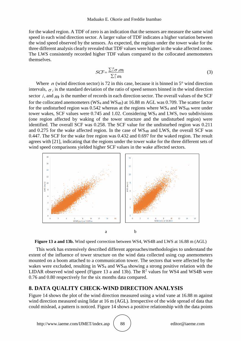
Figure 13 a and 13b. Wind speed correction between WS4, WS4B and LWS at 16.88 m (AGL)

This work has extensively described different approaches/methodologies to understand the

extent of the influence of tower structure on the wind data collected using cup anemometers

mounted on a boom attached to a communication tower. The sectors that were affected by the

wakes were excluded, resulting in WS4 and WS4B showing a strong positive relation with the

LIDAR observed wind speed (Figure 13 a and 13b). The R2 values for WS4 and WS4B were

0.76 and 0.80 respectively for the six months data compared.

8. DATA QUALITY CHECK-WIND DIRECTION ANALYSIS

Figure 14 shows the plot of the wind direction measured using a wind vane at 16.88 m against

wind direction measured using lidar at 16 m (AGL). Irrespective of the wide spread of data that

could mislead, a pattern is noticed. Figure 14 shows a positive relationship with the data points


Measurement


concentrated in 5 major zones though symmetrical. The regions around the blue circles (located

in the left upper corner and right lower corner) indicate that when one instrument measured

values close to 360° at one moment the other instrument recorded values close to 0° at the same

time. The two portions marked with green dash circle lie around ±180° deviation, which is

traceable to the 180° ambiguity issue of the ZephIR 300 as mentioned earlier. The central

portion of the data which lies on the diagonal indicates a region where both instruments

measured relatively the same wind direction. The wind directions and time for a typical day, on

1 April 2014, is illustrated from 00:00 hour to 24:00 hours (Figure 15a). The dashed horizontal

line shows the angle of the wind vane’s boom orientations from the north. The lidar and the

vane see the wind almost from the same angle between 21:10 hours to 11:30 hours. Between

11:30 to 16:30 hours, the direction recorded by the vane appeared to be under tower influence,

hence the unexplained irregular pattern which is different from the more regular pattern

recorded by the Lidar observation. Within the same period, the 180° ambiguity issue of the

ZelphIR 300 is noticed. The Lidar observation is 170° to 180° higher than that of the wind vane

and a similar pattern occurred between 16:30 to 21:10 hours when the Lidar recorded wind

direction that was between 170° to 180° less than that of the vane.

Figure 14 Wind direction correction between wind direction captured using a wind vane and ZephIR

300 at 16.88 m

To further evaluate this, Figure 15b illustrates the plot of the wind direction difference

between the Lidar and wind vane, binned in 10° wind direction intervals and drawn as a function

of the wind direction measured using Lidar (blue line) and wind vane (orange line). The two

graphs are the same, but one is the reverse of the other. In the 1st and 2nd quadrants, the wind

vane measured higher wind direction than the lidar whereas the reverse is the case in the 3rd

and 4th quadrants. The sum of the differences (thick black line) exhibits a sine-function

characteristic between 70° and 270° and a difference up to 34° is noticed in the regions around

70° to 180° and 190° to 270°. The result reveals that winds coming from between approximately

250° and 360° were deflected up to 34° away from the tower structure as recorded by the wind

captured by the vane between approximately 70° and 180°. Similarly, observation shows that

winds coming between approximately 10° to 90° were deflected by the tower structure as

captured by the wind vane records between approximately 190° to 270°.

0

30

60

90

120

150

180

210

240

270

300

330

360

0 30 60 90 120 150 180 210 240 270 300 330 360

Win

d d

irec

tio

n m

easu

red

usi

ng

Lid

ar

at 1

7 m

Wind direction (degree) measured using wind vane at 16.88 m



a b

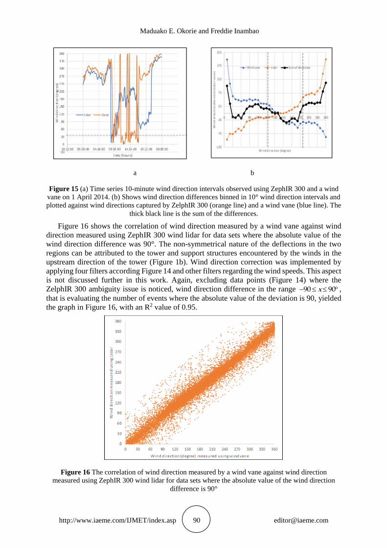
Figure 15 (a) Time series 10-minute wind direction intervals observed using ZephIR 300 and a wind

vane on 1 April 2014. (b) Shows wind direction differences binned in 10° wind direction intervals and

plotted against wind directions captured by ZelphIR 300 (orange line) and a wind vane (blue line). The

thick black line is the sum of the differences.

Figure 16 shows the correlation of wind direction measured by a wind vane against wind

direction measured using ZephIR 300 wind lidar for data sets where the absolute value of the

wind direction difference was 90°. The non-symmetrical nature of the deflections in the two

regions can be attributed to the tower and support structures encountered by the winds in the

upstream direction of the tower (Figure 1b). Wind direction correction was implemented by

applying four filters according Figure 14 and other filters regarding the wind speeds. This aspect

is not discussed further in this work. Again, excluding data points (Figure 14) where the

ZelphIR 300 ambiguity issue is noticed, wind direction difference in the range 90 90x− ,

that is evaluating the number of events where the absolute value of the deviation is 90, yielded

the graph in Figure 16, with an R2 value of 0.95.

Figure 16 The correlation of wind direction measured by a wind vane against wind direction

measured using ZephIR 300 wind lidar for data sets where the absolute value of the wind direction

difference is 90°


Measurement


On the wakes’ impact on some selected resource parameters, removing the sectors within

the waked zone will inevitably reduce the number of available records thus affecting the data

recovery rate (DRR). Based on the boundary defined by speed ratios, DRR for WS4 decreased

by 18.8% and that of WS4B by 15.1%. Similar analysis based on the boundary defined by TIWS4

and TIWS4B found that DRR decreased by 23% and 19.1%, respectively. With the percentages

computed, the representativeness of the data captured is likely compromised. Wake impact on

resource parameters and methods of waked data replacement are not fully explored in this

paper, nonetheless, removing wind speeds that fall within the wake boundary for WS4B and

WS4 lead to slight improvements in the mean wind speeds computed for the full six months

data. For WS4B and WS4, there was a 4.17 % and 0.24 % increase after removing the wake

affected regions. An 11 % decrease of mean value of TIWS4 and a 3.4 % decrease for TIWS4B

was computed.

9. CONCLUSION

The data analysed and compared are data from 10-minute average intervals collected over a

period of six months (01/04/2014 to to 30/09/2014), being the period when the collocated

anemometers at 16.88 m and 64.97 m (AGL) concurrently captured wind data together with

ZephIR 300. To enable an evaluation of the seasonal variations of tower wake effect, the data

from the collocated anemometers captured between May 01 to Dec. 31, 2014, were used.

Different approaches/methodologies were used in identification and evaluation of the extent of

tower and boom wake effects. The traditional speed ratio approach compared the wind speeds

captured for each pair of collocated anemometers (located 120° apart) at 16.88 m and 64.97 m

(AGL) which had been placed on the MTC communication tower at Amperbo. This

arrangement clearly reveals the effect of tower wake on the downstream speed sensors, resulting

in wind speed deficits of up to 49 %. The affected angle range for both pairs of collocated

anemometers at 16.88 m and 64.92 m was approximately between 60° and 65°. The ratio of

turbulence intensities (TIWS4/TIWS4B) reveals that the affected angle span was aproximately

between 65° and 76°, which is higher than the range predicted by mean speed ratio. The range

of angles and extent of wake distortion predicted by TI analysis was not unconnected with

higher perturbations in the wake of tower, and may well prove very valuable in strictly defining

the wake boundries. The severity of wakes on the collocated anemometers differs, a situation

that can be attributed to the presence of secondary support structures and possible positioning

of the speed sensors on different planes (Figure 1d) of the tower, which inevitably presents

different tower porosities and different flow modifications in the vicinity of the tower.

To avoid inverse effects of the speed ratio approach, and to precisely define the wake

affected sectors, the coefficient of determination, R2, was used. The R2 between the WS4 and

WS4B were evaluated in 1° bins of wind vane direction and smoothed with 2° running average.

The boundary of the tower wakes were identified to be the direction sectors which had R2 values

that were less than 2 standard deviations of the mean values of the three non-waked regions

identified. The affected angle in this case were approximately between 60° and 69°. Similar

analysis using TI shows that the R2 between the TIWS4 and TIWS4B binned in 1° wind direction

intervals and smoothed overs 4° running averages, predicted the wake boundary as the direction

sectors which had R2 values that were less than 2 standard deviations of the mean values of R2

of the three non-waked regions. The range of angle affected was beween 60° to 76°. The

correlation analysis shows that the R2 values for mean speeds and TI for the undisturbed regions

were 0.99 and 0.97 respectively, an indication of positive and strong relationship between the

resource parameters from the collocated speed sensors at 16.88 m (AGL).

The variations of wake distortion effects by seasons was evaluated using speed and TI

ratios. For WS4, the winter months (June and July) recorded the highest speed deficits of 55 %



and 56 % respectively between 110° and 115° whereas in December (the summer month) the

smallest value of 40 % at the same angle range was recorded. Considering WS4B, the peak speed

deficits of 33 % and 35 % were recorded in June and July respectively, between 235° and 240°.

December accounted for the smallest value of 23 %. In agreement with the speed ratio analysis,

tower wake influence varied in intensity in seasons of the year. In June and July, the peak winter

months, the ratios of TI varied from 1 to 4.09 and 4.16 respectively at 110° wheras in December,

a summer month, the range was from 1 to 1.8 at the same angle range as WS4B. Similar result

were obtained for WS4 where the ratio of TI varied from 0.40 to 1 and 0.41 to 1 respectively

between 230° and 240°. In December the TI ratio was the smallest with values of 0.72 to 1. The

speed deficit and increase in TI appeared to be directly related to the wind speed. Arrangement

of the collocated anemometers appeared not to be adequate to investigate the booms and

possible speed up effects on the free stream winds captured by any of the speed sensors.

ZephIR 300 enabled the identification of the tower wakes, boom wakes and possible speed

ups effects. The ratio of wind speeds (WS4/LWS and WS4B/LWS) were analysed, drawn as a

function of wind direction measured using a wind vane and then compared. For WS4 and WS4B,

speed deficits up to 50 % and 40 %, respectively were recorded. To identify boom wakes and

speed effects, the speed ratios (WS4/LWS and WS4B/LWS) were drawn as a function of wind

direction measured using ZephIR 300. The speed deficit of up to 47 % less than the Lidar

observed speed was computed around 165° for the South East anemometer (WS4). For WS4B,

speed deficit of up to 32 % less than the lidar wind speed was computed around 285°. The

boundaries of the boom’s wake for both speed sensors were asymmetrical and cantered at a

clockwise orientation from the boom orientation, an indication that winds at Amperbo

predominantly blow in a clockwise direction. For both WS4 and WS4B, a 5 % speed up effect

was noticed between 5° and 20° with a peak at 10°.

Further investigation required the computation of the Root Mean Square Errors (RMSE) to

ascertain the similarity degree of resource parameters. Considering the wind speeds, the peak

RMSE values for the waked regions were 2.63 m/s and 1.39 m/s for WS4 and WS4B, whereas

TI provided 0.35 m/s and 0.14 m/s for WS4 and WS4B respectively. The TI approach

consistently predicted larger wake boundaries than speed ratio analysis. The Tower Distortion

Factor (TDF) and the Scatter Factors (SCF) were consistent with findings in literatures, with

TDF and SCF being higher at wake affected sectors when compared with the undisturbed

regions.

Wind direction analysis clearly revealed the 180° ambiguity ZephIR 300 and possible

deflection of winds. Winds coming from between approximately 250° to 360° were deflected

up to 34° away from the tower structure as recorded by the wind captured by t wind vane

between approximately 70° to 180°. Similar observation showed winds coming from between

approximately 10° and 90° were deflected by the tower structure as captured by the wind vane

records between approximately 190° and 270°.

Wake impact on resource parameters and methods of waked data replacement are not fully

explored in this paper, however, removing wind speeds that fall within the wake boundary for

WS4B and WS4 led to slight improvements in the mean wind speeds computed for the full six

months data. For WS4B and WS4, there was a 4.17 % and 0.24 % increase in mean wind speed

after removing wake affected regions. There was a 11 % decrease of mean value of TIWS4 and

a 3.4 % decrease for TIWS4B.

Finally, different approaches/methodologies were used in identification of tower wake

distortion and definition of wake boundaries from the MTC communication tower used for wind

data collection at Amperbo. Flow modification within the vicinity of the tower due to the

tower’s physical structures and other secondary support structures have significant influence on

the wind speed, turbulence intensity and wind directions. For stringent evaluation of the wake


Measurement


influence, the results show that TI analysis has the potential to accurately define the wake

boundaries and the extent of wake distortion.

ACKNOWLEDGEMENTS

Funding for this project was provided by the Ministry of Foreign Affairs of Denmark, Ministry

of Foreign Affairs of Finland, United Kingdom Department for International Development,

Austrian Development Agency and Namibia Power Corporation. Invaluable support is provided

by Namibia Energy Institute under Namibia University of Science and Technology.

REFERENCES

[1] International Electrotechnical Commission (IEC), Wind Energy Generation Systems – Part

12-1: Power Performance Measurements of Electricity Producing Wind Turbines.

International Electrotechnical Commission (IEC), IEC Central Office 3 rue de Varembé

CH-1211 Geneva 20, Switzerland, International Standard IEC 61400-12-1:2005(E), Dec.

2005.

[2] International Electrotechnical Commission (IEC), Wind Energy Generation Systems – Part

12-1: Power Performance Measurements of Electricity Producing Wind Turbines.

International Electrotechnical Commission (IEC), IEC Central Office 3 rue de Varembé

CH-1211 Geneva 20, Switzerland, International Standard IEC 61400-12-1:2017-03(en-fr),

Mar. 2017.

[3] Orlando, S., Bale, A. and Johnson, D. Experimental Study of the Effect of Tower Shadow

on Anemometer Readings, Journal of Wind Engineering and Industrial Aerodynamics, 99,

2011, pp. 1–6.

[4] Lubitz, W. D. and Michalak, A. Experimental and Theoretical Investigation of Tower

Shadow Impacts on Anemometer Measurements, Journal of Wind Engineering and

Industrial Aerodynamics, 176, 2018, pp. 112–119.

[5] Hansen, M. and Pedersen, B. M. Influence of the Meteorology Mast on a Cup Anemometer,

Journal of Solar Energy Engineering, 121(2), 1999, pp. 128–131.

[6] Stickland, M., Scanlon, T., Fabre, S., Oldroyd, A. and Kindler, D. Measurement and

Simulation of the Flow Field Around a Triangular Lattice Meteorological Mast, Energy and

Power Engineering, 5(10), 2013.

[7] McCaffrey, K. et al., Identification of Tower-Wake Distortions using Sonic Anemometer

and Lidar Measurements, Atmospheric Measurement Techniques; Katlenburg-Lindau,

10(2), 2017, pp. 393–407.

[8] Dabberdt, W. F. Tower-Induced Errors in Wind Profile Measurements, Journal of Applied

Meteorology, 7(3), 1968, pp. 359–366.

[9] Orlando, S. Bale, A. and Johnson, D. A. Experimental Study of the Effect of Tower Shadow

on Anemometer Readings, Journal of Wind Engineering and Industrial Aerodynamics,

99(1), 2011, pp. 1–6.

[10] Cermak J. E. and Horn, J. D. Tower Shadow Effect, Journal of Geophysical Research,

73(6), 1968, pp. 1869–1876.

[11] Fabre, S., Stickland, M., Scanlon, T., Oldroyd, A., Kindler, D. and Quail, F. Measurement

and Simulation of the Flow Field Around the FINO 3 Triangular Lattice Meteorological

Mast, Journal of Wind Engineering and Industrial Aerodynamics, 130, 2014, pp. 99–107.

[12] ZelphIR Lidar, ZP300 Operations & Maintenance Manual, QinetiQ Ltd (UK) ZelphIR

(Z300) Lidar, Uk, Technical report, Feb. 2013.

[13] ZelphIR Lidar, Guidelines for Siting and Comparison of ZephIR Against a Meteorological

Mast, QinetiQ Ltd (UK) ZelphIR (Z300) Lidar, UK, Technical report, Nov. 2013.



[14] Pena A. and Hasager, C. B. Remote Sensing for Wind Energy, Risø National Laboratory

for Sustainable Energy, Technical University of Denmark., Risø–I–3184(EN), May 2011.

[15] Knoop, S., Koetse, W. and Bosveld, F. Wind LiDAR Measurement Campaign at CESAR

Observatory in Cabauw: preliminary results, arXiv:1810.01734 [physics], Oct. 2018.

[16] Jaynes, D., Manwell, J., McGowan, J., Stein, W. and Rogers, A. MTC Final Progress

Report: LIDAR, Renewable Energy Research Laboratory, Department of Mechanical and

Industrial Engineering, University of Massachusetts, 2007.

[17] Siepker, E. and Harms, T. The National Wind Resource Assessment Project of Namibia, R

& D Journal of the South African Institution of Mechanical Engineering 33, 2017, pp. 105-116

.

[18] Schmidt, M., Trujillo, J. J. and Kühn, M. Orientation Correction of Wind Direction

Measurements by Means of Staring Lidar, Journal of Physics: Conference Series, 749,

2016.

[19] Jaynes, D. W., McGowan, J. G., Rogers, A. L. and Manwell, J. F. Validation of Doppler

LIDAR for Wind Resource Assessment Applications, AWEA Windpower2007

Conference, Los Angeles, CA, 2007, p. 16.

[20] Rehman, S. Tower Distortion and Scatter Factors of Co-Located Wind Speed Sensors and

Turbulence Intensity Behavior, Renewable and Sustainable Energy Reviews, 34, 2014, pp.

20–29.

IDENTIFICATION OF TOWER AND BOOM- WAKES USING … · Identification of Tower and Boom-Wakes Using...

Documents

Transcript of IDENTIFICATION OF TOWER AND BOOM- WAKES USING … · Identification of Tower and Boom-Wakes Using...