Identification of Soil Property Variation Using Spectral ... Output/Mila Luleva.pdf · Identifying...
111
Identification of Soil Property Variation Using Spectral and Statistical Analyses on Field and ASTER Data. A Case Study of Tunisia Mila I. Luleva February, 2007
Transcript of Identification of Soil Property Variation Using Spectral ... Output/Mila Luleva.pdf · Identifying...

Identification of Soil Property Variation Using Spectral and Statistical
Analyses on Field and ASTER Data.
A Case Study of Tunisia
Mila I. Luleva
February, 2007

Course Title: Geo-Information Science and Earth Observation
for Environmental Modelling and Management
Level: Master of Science (MSc)
Course Duration: September 2005 - March 2007
Consortium partners: University of Southampton (UK)
Lund University (Sweden)
University of Warsaw (Poland)
International Institute for Geo-Information Science
and Earth Observation (ITC) (The Netherlands)
GEM thesis number: 2005-26

Identification of Soil Property Variation Using Spectral and Statistical
Analysis on Field and ASTER Data.
A Case Study of Tunisia
by
Mila I. Luleva
Thesis submitted to the International Institute for Geo-information Science and Earth
Observation in partial fulfilment of the requirements for the degree of Master of
Science in Geo-information Science and Earth Observation: Specialisation:
Environmental Modelling and Management
Thesis Assessment Board:
Chairperson Prof. Dr A. K. Skidmore
External examiner Prof. P. M. Atkinson
Supervisor Prof. Dr F. D. van der Meer
Member 1 Prof. P. Pelesjö
Member 2 Dr. H. M. A. van der Werff
International Institute for Geo-Information Science and
Earth Observation, Enschede, The Netherlands

Disclaimer
This document describes work undertaken as part of a programme of study at
the International Institute for Geo-information Science and Earth Observation.
All views and opinions expressed therein remain the sole responsibility of the
author, and do not necessarily represent those of the institute.

i
Abstract
Identifying the most suitable and cost- time effective technique for studying soil
properties variation has been a challenge for many soil scientists. Even though the
spectral characteristics of the soil and its constituents have been widely examined,
the use of satellite remote sensing data and ASTER imagery in particular, has been
limited. The aim of this study was to investigate soil properties such as moisture
content, organic matter, electroconductivity, pH, Calcium, Carbonates, Magnesium,
Manganese, Sodium, Potassium, and Iron within similar soil types by ASTER. The
study area was located in South-East Tunisia, chosen mainly due to the limited
presence of vegetation and extensive regions of bare soil. The methodology consists
of chemical and physical composition determination, moving through fine resolution
soil laboratory spectra measurements and development of Partial Least Squared
Regression (PLSR) models to link these results to ASTER imagery. Two ASTER
scenes were selected- winter season, years 2003 and 2005, in terms of gathering
better overview of the current situation. These two have been pre-processed and
classified by Maximum Likelihood (two different band combinations), using the
same techniques and the same regions of interest (training/testing sites), identified
from reference soil map and ISODATA unsupervised algorithm. Three accuracy
assessment techniques were applied in terms of identifying the performance of the
classifications as well as probability levels for correctly classified pixels. It was
established that with 95% confidence, only one out of ten samples was ‘probably’
correctly classified. The spectra collected under laboratory conditions using ASD
FIELDSPEC spectrometer were stored in a spectral library, which was then
resampled to ASTER and, together with the derived spectra from the ASTER scenes,
was input into the PLSR model collectively with the determined concentrations. The
PLSR models resulted in a set of correlations between the properties and the
reflectance values (R2 >0.9 for EC, Ca, Mg). The PLSR coefficients were plotted in
terms of identifying important wavelengths related to the properties. With the
decrease of spectral resolution, these wavelengths were reduced and the final set was
observed mainly in the shortwave infrared region. Even though the findings were
based on limited data available, the conclusions were optimistic, acknowledging the
potential use of ASTER in soil properties prediction and determination. Further work
can emphasise on the use of more soil samples, implementation of different terrain
parameters and selection of number of homogeneous, but with different nature, soil
clusters for sampling.

ii
Acknowledgements
There are so many people that contributed to the completion of this thesis but
unfortunately I have to limit myself to mentioning only some of them.
First of all, I would like to express my greatest gratitude to the academic team
involved in this research. Prof. Freek Van der Meer, thank you very much for all the
help, support, patience and constructive criticism. Your professionalism has
contributed greatly not only to this project but also to the development of my interest
and knowledge in the area of remote sensing. Dr. Ulrik Martensson and Dr. Harald
Van der Werff, thank you for the help and support throughout this journey. Drs.
Boudewijn de Smeth, thank you for the hours you spend in the laboratory
The Tunisian team- Ali, Nejeh and Abderrazak, thank you for making me feel at
home during my stay in your beautiful country. The long and very hot hours we spent
in the field as well as all the help in general, have been much appreciated.
Enormous ‘Thank you’ goes to everyone involved in the development of GEM MSc.
I am extremely grateful that you gave me the opportunity to travel, study and meet so
many great people at the same time.
To all my amazing GEM classmates: I really cannot believe one year and a half has
gone so fast. You guys made it unforgettable. Thank you for everything! I wish you
all lots of luck and great success! Sarika, Yan, Shawn and Chen- I will miss you guys
a lot, especially when I want a nice coffee with a great company in the “Sandy
place”, or a portion of these amazing mushrooms with Chinese leaves- NO spices!! I
will keep quiet about the long hours we spent cooking and baking...
I would like to thank my family and my friends for all the support during those
difficult little moments that everyone has once in a while. Mom and Dad, without
you none of these would have been possible- ‘Благодаря ви за всичко’. Ivo, thanks
for being the best brother ever! Stef and Iain- you guys—there are no words to
explain how grateful I am to you—if one day I can help somebody at least half as
much, I will be the happiest person on Earth!!!
Everyone who helped me, supported me and believed in me- Thanks for everything,
you people made it possible!

iii
Table of contents
Abstract........................................................................................................................ i
Acknowledgements..................................................................................................... ii
Table of contents .......................................................................................................iii
1. Introduction........................................................................................................ 1
1.1. Background.............................................................................................. 1
1.2. Problem Statement................................................................................... 5
1.3. Research Questions.................................................................................. 6
1.4. Research Objectives ................................................................................ 6
1.5. Research Hypotheses ............................................................................... 7
2. Materials and Methods....................................................................................... 9
2.1. Study Area ............................................................................................... 9
2.2. Soil Types and Characteristics Within the Region of Interest ............... 10
2.3. Field Data Collection............................................................................. 12
2.4. Data Processing ..................................................................................... 13
2.4.1. Laboratory Samples Analyses........................................................... 13
2.4.2. Spectral analysis ............................................................................... 14
2.4.3. Image analysis................................................................................... 17
2.4.4. Soil types identification per sample .................................................. 22
3. Results.............................................................................................................. 25
3.1. Laboratory analysis results .................................................................... 25
3.2. Spectral and image analysis ................................................................... 26
3.2.1. Laboratory spectra and CIE diagram ................................................ 26
3.2.2. PLSR on laboratory spectral library.................................................. 27
3.2.3. Image analysis................................................................................... 28
3.3. Soil types and properties identification per sample ............................... 35
4. Discussion........................................................................................................ 39
4.1. Spectral library analysis......................................................................... 39
4.2. Partial Least Squared Regression models .............................................. 40
4.3. ASTER scenes analysis ......................................................................... 44
4.3.1. Spectral profiles per sample.............................................................. 44
4.3.2. Classifications................................................................................... 45
4.4. Soil types identification within the study area ....................................... 49
5. Conclusions...................................................................................................... 55
6. Recommendations............................................................................................ 57
7. References........................................................................................................ 59
8. Appendices....................................................................................................... 63

iv
8.1. Appendix 1: Selected figures and tables ................................................63
8.1.1. Figures ..............................................................................................63
8.1.2. Tables................................................................................................70
8.2. Appendix 2: Field work report...............................................................76
8.3. Appendix 3: Samples photographs ........................................................83
8.4. Appendix 4: Procedures for soil analysis...............................................84
8.5. Appendix 5: Classification Accuracies ..................................................87

v
List of figures
In Text:
Figure 1: Location of the Study Area
Figure 2: Flowchart of data processing methodology
Figure 3: PLSR coefficients from laboratory spectral library
Figure 4: PLSR coefficients: laboratory spectra vs. resampled to ASTER spectra
Figure 5: PLSR coefficients: ASTER 2003 vs. ASTER 2005
Figure 6: Aster classifications outputs
Figure 7: Soil type coverage defined by the classification techniques at different
confidence levels
Figure 8: Soil types according to classification for the sampling points
Figure 9: Soil types according to classification for the test points
In Appendix:
Figure A1: Soil maps
Figure A2: Flowchart of PLSR data arrangement procedure (Wold et al. 2001)
Figure A3: Distribution of sampling points
Figure A4: Eigen values from MNF transformed bands
Figure A5: a) CIE tristimulus curves; b) CIE Chromaticity diagram
Figure A6: CIE diagram and soil sample distribution according to their colour
Figure A7: Spectral signatures derived under laboratory conditions
Figure A8: Spectral profiles extraction from ASTER at each sampling location
Figure A9: Analysis of the three spectral libraries for selected sampling points
Figure A10: Misclassified pixels associated with Lithosols, Brown Lithosols, and
Lithosols/Regosols

vi
List of tables
In Text
Table 1: Results from laboratory analysis and precision assessment
Table 2: Albedo and soil colour analysis
Table 3: Spectral wavelength regions important for the PLSR prediction model of
the properties
Table 4: Image classifications overall accuracy, kappa coefficients and most
successfully classified soil types
Table 5: Validation matrix for sampling points against soil types from ASTER
scenes, 2 classification methods and different probability levels
In Appendix
Table A1: PLSR prediction model assessment from laboratory results and spectral
library
Table A2: PLSR prediction model assessment for the resampled to ASTER library
Table A3: PLSR prediction model assessment for spectra derived from ASTER scene
2003
Table A4: PLSR prediction model assessment for spectra derived from ASTER scene
2005
Table A5: Extraction of soil types from each classification per sample point
Table A6: Extraction of soil types from each classification per test point

IDENTIFICATION OF SOIL PROPERTY VARIATION USING SPECTRAL AND STATISTICAL ANALYSIS
1
1. Introduction
Over the last couple of decades, it has been a challenge to find the most appropriate
technique for studying soil properties effectively and, at the same time, reducing the
time and effort involved in field sampling and laboratory analysis. This has been of a
major concern not only for soil scientists but also environmental managers. In this
respect, the scope of remote sensing has been widely studied, looking more closely at
how the spectral soil response can be linked to various soil properties and
characteristics. Furthermore, as stated by Palacios-Orueta and Ustin (1998), the
relatively high spectral resolutions as well as contiguous placement of bands,
together with the shortwave infrared region of the reflected spectrum offered by most
of the newly launched sensors, create opportunities for the specialists in the field.
Even though, the heterogeneous nature of soil creates a lot of difficulties in terms of
assessing its properties from reflectance spectra, if the spectral response is well-
known, multispectral imagery could be successfully used for this purpose (Ben-Dor
et al 2002).
1.1. Background
As stated by Udelhoven et al. (2003), soil parameters are neither static nor
homogenous in space and time; however, the costs of the analytical procedures are
often a limiting factor when address spatial soil variability especially in large-scale
applications. Reflectance spectra have been used for many years as a source of
information about the variation in the Earth's surface composition (Van der Meer et
al., 2001). Consequently, the soil properties derived from spectra have been studied
long before the 1980s. Many studies have drawn their main emphasis on the visible
and infrared regions of the spectrum- between 0.3 and 2.8 µm (Baumgardner et al.
1985), and the trend has been followed to date, with some relationships established
from data in the thermal and microwave regions (Barnes et al. 2003). The majority
of the absorption features, diagnostic for mineral composition, occur in the short-
wave infrared portion of the wavelength spectrum ranging from 2 to 2.5 µm.
Moreover, Shepherd and Walsh (2002) state that most of the basic physical and
chemical soil properties show high correlation with derivative reflectance values
within the visible and short-wave infrared wavelengths. These authors also suggest
that subtle differences in the spectral shape can serve as a valuable base for

IDENTIFICATION OF SOIL PROPERTY VARIATION USING SPECTRAL AND STATISTICAL ANALYSIS
2
identifying soil properties mainly due to the fact that the soil spectra forms as a result
of the overlap between absorption features of many organic and inorganic
compounds (Shepherd & Walsh, 2002). To a large extent, the changes in the spectral
response, according to Ben-Dor et al. (2003), occur due to changes in soil albedo
and soil chromophores, where the former is strictly related to the physical soil
properties, while the latter – to the chemical. Many researchers have identified clear
relationships between the soil colour, organic matter and iron content, which are also
strongly correlated with the soil albedo. There has been a general consensus that soil
albedo is determined by three main factors: moisture content, surface roughness and
soil colour (Post et al., 2000). In many cases, however, other factors may also
strongly influence the albedo. Soil electroconductivity for example is a property of
the soil affected by not only soil moisture but also dissolved salts content, clay
content, mineralogy and soil temperature. A relationship established between this
soil property and soil albedo can indicate that the latter is influenced by one of the
factors affecting the electroconductivity. Baumgardner et al. (1985) identified that
the differences in moisture content, organic matter, soil texture, iron content as well
as salinity determine most of the spectral responses in this spectrum range.
The presence of organic matter in the soil has been found to decrease the overall
reflectance and result in decrease in the spectral contrast. Consequently, this makes
the relationship between spectral and physicochemical properties much more
difficult to examine (Palacios-Orueta and Ustin, 1998). Furthermore, as outlined by
Palacios-Orueta et al. (1999), organic matter is a crucial indicator not only of soil
erosion but also of soil water holding capacity and permeability. Measurements of
organic matter content in soil have been included in many studies. The wavelengths
identified by Barnes et al. (2003) as ones having strong correlation with organic
matter, are between 0.425 and 0.695 µm, however this is only a case if the soils have
the same parental material. The authors also identified that this relationship could be
affected by the iron and manganese oxides present in the soil. If the soils are from
different parental material, it has been suggested that the middle infrared region
should be examined (Barnes et al. 2003).
On the other hand, the shape of soil reflectance curves, according to Baumgardner et
al. (1985), is affected by the presence of strong water absorption bands at 1.45 and
1.95 µm. Recently, Barnes et al. (2003) have observed that soil moisture is most
effectively correlated to visible and near infrared reflectance of bare soil fields if the
data are collected a few days after rainfall. According to Van der Meer et al. (2001),
the increasing moisture content decreases the overall reflectance of the soil. The

IDENTIFICATION OF SOIL PROPERTY VARIATION USING SPECTRAL AND STATISTICAL ANALYSIS
3
microwave part of the spectrum has also been suggested by some; however, the
process could be highly limited by the presence of vegetation (Barnes et al. 2003).
Salinity of soils has been studied from spectral reflectance as well, where most of the
features seen in the spectrum of saline minerals can be quantitatively measured by
laboratory or field spectroradiometers (Farifteh et al., 2006). It has been found that
saline soils give lower reflectance than non-saline throughout the range between 0.5
and 2.38 µm (Baumgardner et al., 1985). In the case of salt-affected soils, the white
crust that forms on the surface tends to have higher reflectance in the visible and near
infrared part of the spectrum (Barnes et al. 2003). However, as stated by Barnes et
al. (2003), this should not be considered as a clear indicator due to the fact that soils
with high sand content will have a response curve, which has similar shape, in the
visible and near infrared region, to the saline soils.
Soil texture has been studied by many using analysis of spectral reflectance. To
minimise the effect of other properties, Barnes et al. (2003) suggest the use of
combined data from the visible, near infrared and thermal infrared spectra. The
authors also recommended direct field sampling in terms of improving the accuracy
of interpretation of the bare soil imagery. Particle size has been identified to
influence strongly the soil reflectance. As stated by Baumgardner et al. (1985)
referring to an earlier study done by Bowers and Hanks (1965), with the decrease in
particle size, a strong exponential increase in reflectance can be noted, throughout all
wavelengths in the range of 0.4 to 1.0 µm. Although several techniques have been
found relatively efficient in studying soil texture from reflectance properties, it is
important to note that very often only textural classes can be identified from the
spectral response (Barnes et al., 2003).
Many studies have been conducted relating Potassium (K) to spectral response.
Shepherd and Walsh (2002) applied a non-linear regression technique known as
MARS (multivariate adaptive regression spline), to predict the concentration of
exchangeable K and P (Phosphorus) from soil reflectance. The results from the study
were relatively poor however the authors suggest that the relationships are strong
enough to permit discrimination of soils falling above or below a specific threshold
value. It is known, however, that non-polluted soil has concentrations of around 2-
3% for exchangeable K and P. Therefore, the change in the concentration will not be
easily detected using spectral response curves, unless high amounts of these elements
have been artificially added to the soil.

IDENTIFICATION OF SOIL PROPERTY VARIATION USING SPECTRAL AND STATISTICAL ANALYSIS
4
As indicated so far, there is a great amount of literature covering the in-situ
laboratory procedures for estimating and predicting soil properties. These
procedures, however, cannot always be applied, especially when it comes to large or
remote areas. Interestingly, not much has been done on the use and applications of
remote sensing techniques in this field in terms of identifying soil properties, despite
the fact that, according to Baumgardner et al. (1985), studying soil for mapping
purposes with aerial photographs dates from year 1929. Ben-Dor et al. (2002)
identify two general, but very important limitations related to the use of remote
sensing in soil science: only the top few centimetres can be studied and soil
vegetation masks the response from the soil surface. Recently it has been concluded
that multispectral remote sensing is an advanced technique that allows the
identification of targets, in this case soil properties, based on their extensively
studied spectral absorption features, with a near-laboratory quality detection of
reflectance spectra (Ben-Dor et al. 2002). There have been many efforts to include
aerial photographs and satellite images of bare soil in terms of studying organic
matter and phosphorus levels. Lopez-Granados et al. (2005) pointed out that these
approaches were mainly based on linear regression with brightness values from the
blue, green and near infrared bands. Chabrillat et al. (2002), on the other hand,
outline the fact that, unlike multispectral imagery, hyperspectral remote sensing
provides a continuous spectrum for each pixel, which enables the spectral
identification of minerals, rocks, or soils with laboratory-like reflectance
spectroscopy at the remote sensing scale (Chabrillat et al. 2002). Ben-Dor et al.
(2002) also note that since soil is a very heterogeneous material it is more difficult to
apply quantitative analysis to multispectral remotely sensed data.
ASTER (Advanced Spaceborne Thermal Emission and Reflection Radiometer) is a
cooperative effort between NASA and Japan's Ministry of Economy and Industry.
The instrument captures high spatial resolution data in 14 bands from the visible to
thermal infrared wavelengths and provides stereo viewing capability for digital
elevation model creation. It consists of three separate subsystems- VNIR, SWIR and
TIR. The VNIR (visible and near infrared) operates at the visible and near infrared
wavelengths with a resolution of 15m, while the SWIR (short wave infrared) has a
resolution of 30m and operates in six spectral bands in the near infrared region. The
TIR (thermal infrared) has a resolution of 90m and obtains data in 5 bands all in the
thermal infrared region (California Institute of Technology, 2006).
In a study by Chang & Islam (2000), soil moisture and brightness temperature have
been determined from ASTER imagery, in terms of identifying different soil types by

IDENTIFICATION OF SOIL PROPERTY VARIATION USING SPECTRAL AND STATISTICAL ANALYSIS
5
examining a sequence of remotely sensed images. A great disadvantage of the
procedure, however, is the fact that the results contain information only about the
near-surface soil properties. The procedure is valuable when performed on remote or
large areas. ASTER imagery has also been used in a study by Apan et al. (2002),
identifying different soil attributes, soil colour and texture in particular, as well as
land cover types. Reasonable separability has been indicated in ASTER Bands 2 and
8, for both soil colour and texture. The authors also point out that SWIR band ratios
are not useful for separability purposes.
1.2. Problem Statement
Spectrometry under laboratory conditions has been proven to be rather effective, and
therefore has been used in many soil related studies. Remote sensing techniques,
however, have not been applied to such extent, especially when it comes to
multispectral imagery such as ASTER. This is mainly due to the difficulties related
to the choice of study area clear from vegetation and containing most of the variation
in the top 10 cm as well as the coarser resolution provided by the sensor compared to
the laboratory spectra. Moreover, as stated by De Jong & Epema (2001), reflection
measurements, when taken in the field, represent a complex mixture of soil
components, varying soil surface conditions and atmospheric effects. The main
purpose of this study, therefore, is to explore the possibilities of using this type of
imagery in identifying direct and indirect relationships between soil constituents
measured in the laboratory, spectrometer measurements also performed in the
laboratory, and ASTER data.

IDENTIFICATION OF SOIL PROPERTY VARIATION USING SPECTRAL AND STATISTICAL ANALYSIS
6
1.3. Research Questions
• Can soil properties, such as moisture content, organic matter and Calcium,
Potassium, Magnesium, Manganese and Sodium concentrations, at trace
level, be determined from the spectral response derived under laboratory
conditions as well as from ASTER images?
• Can relationships obtained from laboratory analysis, both direct and
indirect- via the spectral response, between the above mentioned soil
properties, be established with analyses of ASTER images?
• Is ASTER imagery suitable for detecting variation of the chosen soil
properties over small areas, considering the similar nature of different soil
types?
1.4. Research Objectives
• To identify the most suitable soil properties for analysis according to the
characteristics of the study area as well as the literature.
• To analyse two ASTER scenes in terms of identifying variation in soil types
and respectively soil properties associated with them.
• To create spectral libraries of all soil samples in terms of identifying unique
absorption features and variation between the samples, from spectral
responses obtained under laboratory conditions as well as these extracted
from ASTER imagery.
• To identify relationships between certain wavelengths from the spectrum
and the absorption features associated with them, using PLSR models and
assess their applicability.
• To evaluate and combine the results from the image analysis with those
derived under laboratory conditions, in terms of achieving maximum
performance of the technique.

IDENTIFICATION OF SOIL PROPERTY VARIATION USING SPECTRAL AND STATISTICAL ANALYSIS
7
1.5. Research Hypotheses
• The presence of soil properties such as moisture content, organic matter and
Calcium, Potassium, Magnesium, Manganese and Sodium concentrations in
soil can be derived from the spectral response measured in the laboratory as
well as from ASTER images.
• Relationships can be derived from laboratory analysis, both direct and
indirect, between the above mentioned soil properties, and be established
with analyses of ASTER images.
• ASTER imagery is suitable for detecting variation of the chosen soil
properties over small areas.


IDENTIFICATION OF SOIL PROPERTY VARIATION USING SPECTRAL AND STATISTICAL ANALYSIS
9
2. Materials and Methods
2.1. Study Area
The study site is located in South-Eastern Tunisia (see figure 1). The area is 16.206
km2, with top left and top right coordinates respectively x: 601530 y: 3729154 and x:
602546 y: 3728787 (WGS 84, UTM zone 32). It is located in the Matmata
Mountains through the Jeffara plain into the Gulf of Gabes. The region has been
chosen not only due to the great interest from governmental and non-governmental
organisations, but also because of the relatively large areas of bare soil. It is
characterised by typical Mediterranean climate with maximum temperatures reached
in the period between June and August (48ºC), whereas the coldest temperatures are
measured between December and February. Due to the proximity to the sea, the
climate of the study area slightly differs from the typical arid or semi-arid. The
rainfall is very irregular and ranges between 150-240mm with an average of 30 rainy
days per year (September/October). This low rate of rainfall combined with the high
temperatures in the summer result in very high potential evapotranspiration up to
around 1321mm. The yearly climatic water balance is almost negative. There are two
major geological landscapes- the Djabel Matmata and the Jeffara. The former is
characterized by an average altitude of 500 meters (northern altitudes reach more
than 600). The latter, on the other hand, reaches the highest level of 100m above sea
level. The geology is comprised of continental and marine formations, the most
recent one dating from recent Quaternary. There are two main soil groups- Aridisols
and Entisols, with very small depth, with big patches of bare rock due to extensive
erosion. The area is mainly rural, with livestock and rain fed farming activities. A lot
of the land is agricultural, mainly olive trees plantations. The population of the
region is estimated at around 62 00 inhabitants spread across 13 imadas
(administrative areas) divided into 5 ethnic groups.

IDENTIFICATION OF SOIL PROPERTY VARIATION USING SPECTRAL AND STATISTICAL ANALYSIS
10
Figure 1: Location of the Study area.
Source of map: http://www.africa-expedition.com/images/ct/tunisia-map.jpg [accessed 5/01/2006]
2.2. Soil Types and Characteristics Within the Region of Interest
The diversity of the soil types within the study area is limited. To come to this
conclusion, two soil maps have been studied in terms of initially identifying the
variation. The older version has been produced by the Soil Division of the Tunisian
Ministry of Agriculture in year 1973. The scale of the map is 1:500,000. The second
map, produced in year 1986, has been prepared by the ACSAD service of mapping
in scale 1:1,000,000 (Figure A1- Appendix 1.1). The types of soils as well as their
codes are explained below. The description of the soil maps is provided by the Soil
Survey Staff (1999), and it is done in numerical order per class, taking into account
the units used on the soil map from 1986.
Aridisols are soils with limited moisture content and holding capacity. Due to runoff
or a very low storage capacity the soil moisture regime is aridic, despite the fact that
during periods of heat, the soil water is held at potentials less than the permanent
wilting point or has a great content of soluble salts caused by the extreme imbalance
between evapotranspiration and precipitation. Tunisia’s main soil group is the

IDENTIFICATION OF SOIL PROPERTY VARIATION USING SPECTRAL AND STATISTICAL ANALYSIS
11
Aridisols, covering 75% of the Southern part of the country, and having 21
subclasses in total. Within the area of interest, covered by the ASTER scenes (60 x
60 km), there are 5 soil sub-classes (see Figure A1-Appendix 1.1). These include
typic Salids (codes 4 and 5-Figure A1b), typic Paleorthids (code 8), which type is
also associated with the sampling study area, typic and petrogypsic Gypsids, or also
known as Gypsiothords (code 10 and 14 respectively), typic Calcids (code16 and
18). The Salids (also referred to as Halomorphs in different classifications) are most
commonly found in depressions or closed basins in the wetter areas bordering the
desserts. These are usually associated with accumulation of excessive amount of
salts, more soluble than gypsum, with typical electroconductivity of 30 µS/cm. If this
type of soil is used for agriculture, the salts are usually leached out. Paleorthids are a
class removed from the revised legend produced by USDA; however the main
characteristics of this type are stony soils, prominent to Calcium Magnesium
encrusting (Ca/Mg) with relatively low salts content. Gypsids are soils that have
gypsic or petrogypsic horizon with its upper boundary within 100cm of the soil
surface. These are characterised by accumulation of gypsum that takes place initially
as crystals aggregates in the voids of the soil. These aggregates build up, which
process results in displacement of the enclosed soil material. Some of the Gypsids
are characterised by a calcic horizon which overlays the gypsic horizon. The last
subclass of the Aridisols found in the area of interest is the Calcids. These are
developed from Calcium Carbonate as a parent material. Precipitation tends to leach
or move the carbonates to great depth. The upper boundary of the calcic horizon is
usually within 50cm of the soil surface. If the soils are irrigated or cultivated,
micronutrient deficiencies are normal.
The second main group of soils is the Entisols (also referred to as Lithosols). These
have little or no evidence of the development of pedogenic horizons, mainly
explained by the fact that in many landscapes the soil material is not in place long
enough to form these horizons. These soils are present either on steep slopes which
are actively eroded, or on flood planes, receiving new deposits of alluvium at
frequent intervals. The only features common to all soils under the order of Entisols
are the virtual absence of diagnostic horizons and the mineral nature of the soils. It is
possible, due to the specific location and different composition, these soils to be
mixed with other soil types resulting in sub-classes such as Brown Lithosols,
Lithosols/Regosols, etc. These, however, are essentially Lithosols, with small
number of additional constituents. The most clearly defined two subclasses
representing this diverse soil group in the region of interest are Torriorthents (code
33) and typic Torrifluvents (code 34), referred to as ‘fluvial soil’ further in the

IDENTIFICATION OF SOIL PROPERTY VARIATION USING SPECTRAL AND STATISTICAL ANALYSIS
12
discussion. The typic Torriorthents are shallow to weakly cemented rocks. Some are
moderately deep or deep to hard rock and are extremely dry. These are mainly
present on gently slopes where the sediments are recent and have little organic
carbon. On the other hand, the Torrifluvents are the Fluvents of the arid climates.
Characterized by aridic moisture regime, these soils have higher pH and are mainly
calcareous; however some could be salty depending on their location. The typic
Torrifluvents are the driest Fluvents. These are defined by big cracks and
slickensides, or wedge-shaped aggregates. In their upper 75cm, they do not have a
deposit of pyroclastic minerals (Soil Survey Staff, 1999).
2.3. Field Data Collection
The fieldwork was spread over 2 weeks between the 15th
and 30th
of September
2006, when the first was associated with visual inspection and selection of the study
area. Information about particular soil features and processes such as soil encrusting
formations, erosion rate and debris formation, vegetation characteristics and
seasonality (if any), was also obtained. The study area was selected according to the
following criteria: Areas with no mixture of soil types, availability of bare soil (no
vegetation and no bare rock), and easy access.
The sampling procedure is clustered random sampling. Thirty five soil sampling
units were collected. Six duplicate samples for accuracy assessment of the chemical
analysis were also located at every fifth location. The locations of the sampling units
were selected according to randomly generated coordinate pairs within the study area
(defined by the watershed and the Matmata Mountain)- see Figure A3- Appendix
1.1. Around 200g of soil material was collected at each location and placed in paper
and plastic bags for storage.
The measurements in the field included: location the sampling units (using GPS),
measurements of reflectance using ASD FIELDSPEC spectrometer (not included in
the analysis due to the missing measurements in the SWIR region), pH, and
identification of soil colour using Munsell colour chart. A record of these
characteristics as well as GPS accuracy and projection was kept and it is attached in
Appendix 2. The grain size was not measured in the field due to the many lumps of
soil that have occurred because of the high temperatures. A soil map was not
available at the time of sampling, and therefore soil types were identified after the
field work. Any clear remarks that were considered critical for the analysis (e.g.
vegetation, weather conditions) were noted and are also included in Appendix 2.

IDENTIFICATION OF SOIL PROPERTY VARIATION USING SPECTRAL AND STATISTICAL ANALYSIS
13
2.4. Data Processing
The methodology of the data processing is displayed on Figure 2. Each one of the
stages is described in more details further in the text.
Figure 2: Data Processing flowchart. The numbers correspond to the appropriate
section in the text
2.4.1. Laboratory Samples Analyses
Out of the 35 soil samples, the geochemical laboratory analyses were performed on
only 9 (plus one duplicate) of them transported to the Netherlands, due to financial
and time constraints. The analysis of the soil in the laboratory included analysis of
pH, electroconductivity, moisture content, organic matter, as well as chemical
concentration detection of Calcium (Ca), Magnesium (Mg), Manganese (Mn),
Sodium (Na), Potassium (K) and Iron (Fe). The carbonate concentrations have also
been estimated.
A factor, which strongly affects the spectral response of soil, is the soil structure and
grain size. In the laboratory this has been established, where the larger than 2mm
fractions have been placed in dishes and observed. The large lumps, originally

IDENTIFICATION OF SOIL PROPERTY VARIATION USING SPECTRAL AND STATISTICAL ANALYSIS
14
identified in the field, have not been identified due to the fact that they have broken
down during the transportation and/or sieving. The large particles found in the
laboratory had a diameter of around 1 cm. The procedures applied on the samples
can be found in Appendix 4 or referring to ISRIC Technical paper 9, (Van Reeuwijk,
2002). The concentrations of Ca, Mg, Mn, Na, K and Fe have been detected using
Induced Coupled Plasma- Optical Emission Spectrometer (ICP-OES). The actual
procedures followed during the laboratory analysis are included in Appendix 4,
while the results are summarised in Table 1. Iron concentrations are not included in
the table due to the fact that they have been found to be lower than the detection limit
of the apparatus. Records of the results have been kept and these have then been
implemented into the following stages of the analysis.
2.4.2. Spectral analysis
2.4.2.1. Laboratory spectra
Spectral analyses of the soil have been performed in laboratory conditions using
ASD FIELDSPEC spectrometer. Albedo and soil colour analysis have also been
done using special extension to ENVI software and a device-independent colour
space, originally developed in 1931 by the Commision Internationale de l’Eclairage
(CIE). It is based on the tristimulus colour theory of the human vision (Van der
Werff, 2006) and it has been accepted internationally as a standard for colour
measurements (De Jong & Epema, 2001). The relationships between the bands and
the soil properties have been studied using simple statistical correlations. Partial least
squared regression models (PLSR) using each of the produced spectral libraries
produced, have been run in terms of linking the laboratory spectra to the ASTER
images.
2.4.2.2. CIE diagram
CIE diagram and special extension to the ENVI software have been used. The
program separates the colour form the albedo providing coordinates for referencing
with the CIE diagram and at the same time calculating the percentage albedo. As
described by Mainam (1999), the system uses a set of imaginary XYZ primaries, also
known as tristimulus values that allow most colours, to be defined by a triplet of
these primaries. According to Van der Werff (2006), the CIE standard observer
shows how much of each primary would be used by an average observer to match
each wavelength to light. For the computation of the XYZ tristimulus values, the
tristimulus curves (Figure A5a) are integrated over a spectrum. To plot the colours
on a two-dimensional graph (such as a chromaticity diagram- Figure A5b),

IDENTIFICATION OF SOIL PROPERTY VARIATION USING SPECTRAL AND STATISTICAL ANALYSIS
15
chromaticity coordinates can be used. These are colour definitions independent of
the luminance (Y) and are calculated by a normalization of the tristimulus values
(XYZ), Van der Werff (2006). More detailed description of the procedure is given
by Brown & Feringa (2003). In this research, the CIE coordinates used are x, y
(chromaticity coordinates) and Y (luminance). The main purpose of these analyses
was to estimate the variation of albedo and soil colour between the samples, which
then determines the pre-processing techniques applied on the spectra prior to Partial
Least Squared Analysis (see next section).
2.4.2.3. PLSR
PLSR (Partial Least Squares Regression) was originally developed by Wold (1981)
and it provides quantitative multivariate modelling methods, with inferential
possibilities similar to multiple regression, t-test and ANOVA. It can analyse data
with strongly correlated x variables, and at the same time model several response
variables. PLSR is a way to estimate parameters in a scientific model, which
basically is linear. This model, like any other scientific models, consists of several
parts: the philosophical, conceptual, the technical, the numerical, the statistical and
so on. It is important to note that before the analysis, the X and Y variables are often
transformed to make their distributions be fairly symmetrical. Furthermore, the result
from the method depends highly on the scale. In this respect, with the appropriate
scaling, the focus of the model could be on more important Y-variables and use
experience to increase the weights of more informative X variables. However, in the
absence of knowledge about the relative importance of the variable, the standard
multivariate approach is to, firstly, scale each variable to unit variance by dividing
them by their standard deviation, and secondly, centre them by subtracting their
averages (a process also called auto-scaling). This corresponds to giving each
variable the same weight or the same prior importance in the analysis (Wold et al.
2001). The latter is also strongly recommended for ease of interpretation and for
numerical stability. The PLSR data arrangement procedure is displayed in Figure A2.
There are a number of assumptions that are made related to PLSR: the investigated
system or process is influenced by just a few underlying variables (latent variables).
Both X and Y variables are assumed to be realisations of these latent variables and
are not therefore considered independent. In spectroscopy, it is clear that the
spectrum of a sample is the sum of the spectra of constituents multiplied by their
concentrations on the sample. Furthermore, any data analysis is based on the
assumption of homogeneity. This means that the investigated system or process must
be in a similar state throughout all the investigation, and the mechanism of influence

IDENTIFICATION OF SOIL PROPERTY VARIATION USING SPECTRAL AND STATISTICAL ANALYSIS
16
of X and Y must be the same, which limits the diversity of the variables. X should
contain a quantitative description of the variation in chemical structure between the
investigated compounds. The objective is to understand the variation of Y.
There are some limitations related to PLSR models. Udelhoven et al. (2003) point
out that when the spectra is normalised, there is a clear reduction in the spectral
albedo variations due to grain size differences between the soil samples. Typically,
the small soil surface variations and micro shadows have a large impact on the
measurements which cannot be eliminated by simple spectra pre-treatment. Another
reason for different PLS results could be unequal distribution of nutrients and water
content (Udelhoven et al., 2003). It has been found that on no account the achieved
results can be compared to measurements of the soil surface taken by remote
operating system. If up-scaling is planned, factors such as the atmospheric
transmission path as well as larger spectrally mixed footprints are taken into account.
PLSR has been performed on the measured variables and wavelength range between
500 and 2500nm, using the 10 samples analysed in the laboratory. The software
used for the analyses is ParLeS version 2.1a (Viscarra-Rossel, 2005). The produced
prediction model, as stated by Scholte (2005), is a set of equations (or PLSR
factors), computed as linear combinations of the spectral amplitudes, by using a
regression coefficient for each wavelength position. Therefore it is clear that the
quality and accuracy of the prediction model strongly depends on the pre-processing
techniques, such as scaling or auto-scaling of the data, detection of outliers and also
the number of factors used in the model. In more detail the importance of the pre-
processing is discussed in Scholte (2005). The best training set has been achieved
when five factors are used and the spectra is normalised. Here the normalisation has
been applied in terms of removing the albedo effect, due to the fact that from the CIE
analysis, the albedo has shown little variation between the different samples. A
number of techniques for accurate determination of the optimal number of factors
have been discussed in the literature (Davies, 2001; Scholte, 2005). The smoothing
technique applied to the library derived under laboratory conditions is Savitzky-
Golay filter, second polynomial. This function performs a local polynomial
regression on a distribution to determine the smoothed value for each point (Savitzky
& Golay, 1964). The main advantage of this filter is the fact that the features of the
distribution (relative maxima, minima, width) are preserved. The smoothing
technique proven to be more effective for the libraries derived from the two ASTER
scenes is Median Filter. This is a non-linear digital filtering used for noise removal,
by examining a sample and assessing if it is representative or not.

IDENTIFICATION OF SOIL PROPERTY VARIATION USING SPECTRAL AND STATISTICAL ANALYSIS
17
The results from the PLSR analyses are a set of calculated values (summarised in the
results section). These include the root mean square error (RMSE), ratio of
prediction to deviation (RPD) and mean and relative mean absolute errors (MAE),
where only the first two are used for the assessment of the models performance.
Additionally, the R2, or also known as coefficient of determination, has been
estimated, showing the strength of statistical correlations between the measured in
the laboratory properties concentrations and the models predictions. The RPD
values together with the R2 have been used in terms of assessing the accuracy of the
predicted Y variables. According to Williams (2001), to indicate good prediction of
the model the RPD value should be higher than 2.5 while the R2 should be estimated
0.91. Viscarra Rossel (2005) provides a classification which defines the quality of
the predicted value with the PLSR software. This is stated under each of the tables
containing the results from these analyses. The procedure has been applied on the
laboratory derived spectral library, the resampled to ASTER spectral library, as well
as on the spectra measured from the ASTER scenes after processing, in terms of
identifying the effect of the reduction of spectral resolution. The produced PLS
regression coefficients were then plotted for each property of interest in terms of
identifying the most significant wavelength regions for the prediction of the soil
constituents. The results from these analyses have been combined with those from
the following image manipulations (see section 2.4.3 and Figure 2), in terms of
identifying and predicting accurately the soil properties of interest (see section
2.4.4).
2.4.3. Image analysis
Two ASTER scenes have been acquired, same season (winter) but different years
(2003, 2005), covering the same area. The raw 2A type images have been
georeferenced, and the Digital Elevation Models extracted from them. The softwares
used for the analysis are Arc GIS 9.1 and ENVI 4.2. A number of analytical
techniques have been used in terms of identifying soil types and properties, as well as
variation between and within soil classes. The purpose of using two ASTER scenes
is not to detect changes in soil composition or land cover changes, but rather to
minimise effects that were not identified by the pre-processing techniques. This is
done by comparing and combining the information from the two.
2.4.3.1. Atmospheric correction
Atmospheric correction was required in terms of converting the radiance values into
reflectance. The procedure originally chosen for this was ENVI FLAASH (Fast Line-
of-sight Atmospheric Analysis of Spectral Hypercubes). This is known as the first-

IDENTIFICATION OF SOIL PROPERTY VARIATION USING SPECTRAL AND STATISTICAL ANALYSIS
18
principles atmospheric correction modelling tool for retrieving spectral reflectance
from radiance images. It corrects wavelengths in the visible through near infrared
and short wave infrared range. In terms of achieving faster and more efficient
performance of the operations, originally the image was planned to be resampled to a
smaller area that covers only the study area and some surrounding regions. This
procedure was applied to both scenes; however, due to the extensive cloud cover, not
removed after the atmospheric correction, over the scene from year 2005, it did not
result in useful output and therefore all analyses were performed on full scene
coverage (wherever possible). Unfortunately, the results produced were not
satisfactory and therefore other techniques were examined.
Log Residuals as well as Internal Average Relative Reflectance (IARR) calibration
tools were then applied in terms of obtaining the optimal atmospheric correction
technique. The Log Residuals is used when there is a need of solar irradiance,
atmospheric transmittance, instrument gain, topographic effects and albedo effects
removal from radiance data. The result is a pseudo reflectance image, based on in-
scene statistics that could be used in absorption features identification. In terms of
defining the logarithmic residuals the input spectrum is divided by the spectral
geometric mean, and then divided by the spatial geometric mean. The spectral
geometric mean is the mean of all bands for each pixel and it is used to remove the
topographic effects while the spatial geometric mean is used because the
transmittance and other effects are considered multiplicative. The spatial geometric
mean is the mean of all pixels for each band and accounts for the solar irradiance,
atmospheric transmittance and instrument gain (ENVI 4.2, 2007). On the other hand,
the IARR is used to normalise images to a scene average spectrum. It is found to be
effective for reducing image data to relative reflectance in an area where no ground
measurements exist and little is known about the scene. It has proven to work best in
arid areas with little or no vegetation. The algorithm is designed to calculate an
average spectrum from the entire scene and use it as a reference spectrum, which is
then divided into the spectrum at each pixel of the image. The method found to be
the most useful and give the most accurate (similar to the resampled library) results
is the Log Residuals algorithm which was chosen for the analysis.
2.4.3.2. Histogram matching
In terms of equalising (or make it as close as possible) the brightness of both scenes,
histogram matching was performed. The function automatically matches the
histogram of one image to another, resulting in a histogram of the display, where the
function has started, matching the source histogram (ENVI Help, 2006).

IDENTIFICATION OF SOIL PROPERTY VARIATION USING SPECTRAL AND STATISTICAL ANALYSIS
19
2.4.3.3. Minimum Noise Fraction
Minimum Noise Fraction (MNF) has been applied to exclude the bands from the
ASTER scenes that contain noise. This is essentially a sequence of two principal
component transformations. It is assumed that the data for each pixel consists of
signal and noise, where the adjacent pixels contain the same signal but different
noise (Zhou et al. 2005). The resulting MNF bands represent linear combination of
the original spectral bands. The first MNF band contains the largest percentage of
data variance and the highest spatial coherence, the second contains the second
largest eigenvalue and coherence and so on until reaching the last band, which is
essentially noise-dominated and has the least variance. The MNF bands included in
this study are bands 1 to 4, which are most coherent and provide noise-filtered
datasets.
2.4.3.4. Spectral profiles per sample
The spectral signatures have been measured per sampling point, from the ASTER
scenes. These, then have been examined in terms of recognising main regions of
variation between the samples as well as common absorption features that coincide
with the peaks and sinks outlined by the PLSR analyses (as stated earlier).
2.4.3.5. Image classifications
A number of classifications have also been performed on both images. The purpose
of this is to define the distribution of the different soil types across the area of
interest. The results are then implemented into the following stages of the method
(see figure 2) in terms of identifying and predicting the soil properties. ISODATA
(Iterative Self-Organising Data Analysis Technique) unsupervised classification was
chosen in terms of identifying areas suitable for training sites, while Maximum
Likelihood supervised classifications have been done using ASTER bands 1-9 and
MNF bands 1-4. The results from the supervised classifications were then compared
in terms of assessing the accuracy.
ISODATA is an unsupervised classification scheme, developed with empirical
knowledge gained through experimentation, which requires relatively little
information. Because of the nature of this approach, many problems may emerge.
One of them, typical for all unsupervised image classification techniques, is the fact
that certain proportion of the generated clusters cannot be labelled as an
informational class and therefore the pixels should be excluded from the image or
reclassified (Klein, 2006). Another problem is that, unless the number of desired
classes is well-known, the choice is usually a guess that does not necessary lead to

IDENTIFICATION OF SOIL PROPERTY VARIATION USING SPECTRAL AND STATISTICAL ANALYSIS
20
the desired outcome. Nevertheless, the classifier was used so that a general idea
about the area is obtained. Applying unsupervised classification method before the
supervised allowed the identification of the most common and the most insignificant
classes. The result served as a base for the definition of the training sites. The most
homogeneous areas were compared against the topographic map. The ones identified
as bare soil have been checked with the available soil map from year 1973 (scale
1:500000) and have been used as the so-called ‘Regions of Interest’ in the maximum
likelihood classification.
Maximum Likelihood supervised classification algorithm has been chosen for this
stage of the analysis. It considers the cluster centre as well as its size, shape and
orientation, by calculating a statistical distance based on the mean variance and
covariance matrix of clusters. The main assumption behind this classification
technique is that the statistics of the clusters have a Gaussian distribution. This
method for image classification has been used by many and it is known to give the
most accurate results (Gomez et al., 2005). Another reason for the choice of this
classifier over others is the lack of soil variability within the study area. It allows
more accurate classification of the mixed pixels typical for areas located on the
borders between two different soil classes.
Two band selections have been used, chosen according to previous studies on soil
image classifications. The band combination includes all visible and infrared (one to
nine) ASTER bands, since not only it is identified by Apan et al (2002) that all
ASTER bands contain information about soil attributes, but also due to the fact that
different band combinations and ratios were tested and produced poorer results due
to the nature of the soil types in the area. The second method uses the first four
Minimum Noise Fraction (MNF) bands, found to contain 98% of the de-noised
information. To avoid confusion between the results from the two approaches in
ASTER image classification, the former will be referred to as Maximum Likelihood
(MaxLik) and the latter as MNF ASTER, although both procedures are Maximum
likelihood classifications.
The accuracy assessment of the classifications has been performed applying three
different techniques: assessment of the accuracy according to the regions of interest
(training sites for each class), assessment of accuracy according to the soil map from
year 1973 and examination of the rule images produced prior to the classifications.
Realistically, the first two procedures are relatively unrepresentative due to the fact
that the regions of interest (training and testing sites) are selected according to the
same soil map which is later used for the accuracy assessment. Furthermore, this soil

IDENTIFICATION OF SOIL PROPERTY VARIATION USING SPECTRAL AND STATISTICAL ANALYSIS
21
map is produced 30 years prior to the date of production of the older ASTER scene
(2003). Therefore, differences outlined from the classifications, and considered
inaccuracies, could be simply detected changes. In this sense, the third accuracy
assessment procedure was performed, implementing the use of Rule images. Each
pixel in a rule image represents the similarity between the corresponding pixel in the
image to a reference spectrum (Debba et al. 2005), which in this case are the regions
of interest selected to represent the soil types. The digital number (DN) value
represents the angular distance in radius between each pixel spectrum and the
reference. The user defines a threshold, according to a probability level, and if the
angular distance is smaller than the defined threshold, the pixel is assigned to the
category of the respective reference material (Debba et al. 2005).
Ultimately, to assess what is the probability a particular pixel to be assigned to the
correct soil type class, the classification methods were tested against different
probability levels at 75%, 85% as well as 95% degree of confidence. The limitation
here is also related to the selection of the training and testing sites, which ultimately
leads to the conclusion that the separability and detailed investigation prior to the
selection of the regions of interest are crucial. In ENVI 4.2, this procedure is done,
plotting the DN values on a histogram and calculating the threshold value for each
class. This is followed by calculating the basic statistical parameters such as mean,
median, mode, standard deviation as well as the percentage area covered by the
classes taking into account the probability level.
Due to the limited number of validation points, the rule images have been resized to
the region covered by the selected study area and only the performance of the soil
types known to be found in this area (from the soil map) have been tested. Figure 7
is produced in terms of comparing the results from the classification techniques as
well as the performance of each ASTER scene. It is important to note that the
percentages allocated to each soil type do not add up to 100%, which means that the
rest of the area should be covered by a different soil type, or the pixel simply could
not be allocated to any class due to spectral mixing.
Furthermore, the 9 validation points were tested against the results. For this purpose,
a validation matrix was created (see Table 5). Each point is tested against this matrix.
If the point is classified as one soil type on both images by both classification
techniques (receiving 4 validation units), the soil type would be correct for the
confidence level at which the point is tested. Respectively, if one of the classification
techniques performed differently for only one of the scenes, therefore the point will
be assigned with a validation unit of 3, and will fall into class ‘probably classified
IDENTIFICATION OF SOIL PROPERTY VARIATION USING SPECTRAL AND STATISTICAL ANALYSIS
22
correctly’. The procedure continues by assigning 2 units (‘possibly classified
correctly’) or 1 ‘not classified correctly or belongs to a different class’. The points
with assigned values of 2 and below are considered to fall on mixed pixels, being
defined by a spectral mixture which prevents the classifier to perform accurately.
The validation plot represents not only the difference between the two ASTER
scenes and the performance of the classifications, but also the number of classes, per
validation point, which are supposed to be found within the study area. The
assessment of this has been done so that if a point falls completely outside any of the
predicted classes, a validation unit of 4 is not assigned to it, but rather it receives a 0.
The accuracy assessments of the classifications play a crucial role when it comes to
soil types/properties identification. The results from these procedures have then been
combined with those from the previous analyses in terms of predicting the presence
of the properties of interest (see Figure 2). Accurate soil type identification allows
better determination of the expected soil properties and therefore contributes to the
explanation of any anomalies that may occur during the process.
2.4.4. Soil types identification per sample
The soil types per sampling unit have been extracted not only from the soil maps but
also from the classifications in terms of identifying the performance capabilities of
the techniques. To evaluate the use of ASTER imagery in identifying soil types and
respectively the soil properties discussed earlier (organic matter, moisture content,
electroconductivity, carbonates, calcium, potassium, magnesium, manganese, and
sodium), the classifications and the reference soil maps have been used. This process
involved outlining the study area onto the classification images and the soil maps
followed by comparison of the results for each of the sampling points.
A number of limitations with this technique should be mentioned before any
conclusion is drawn. These are: only 9 soil samples analysed in a laboratory (plus
one duplicate at location A30), the scale of the map used for validation is 1:500000,
while the resolution of ASTER imagery in the VINR is 15m, and 30m in the SWIR.
Here it is important to note that although two soil maps are available, the one with
finer scale was chosen. Furthermore, the accuracy of the soil map has not been
recorded and consequently, this may result in misinterpretation. Therefore, any
points that fall on, or are located near the border between soil types on the map, may
be misclassified. If there is such case, the laboratory results, the results from the
PLSR models as well as the characteristics of the soil types will be the primary factor
in terms of drawing the appropriate conclusion. Another drawback is the cloud

IDENTIFICATION OF SOIL PROPERTY VARIATION USING SPECTRAL AND STATISTICAL ANALYSIS
23
formation present on the scene from 2005, because of which the accuracy of the
classifications in the region where the clouds are, is poor. The same procedure has
been applied for the rest of the samples, which have not been analysed in the
laboratory, in terms of predicting to what extent the technique can be applied on
unknown locations. If there is mismatch between the classification results and the
soil map, instead of laboratory results, the PLSR results have been used, relating the
spectral response to the soil properties of interest.

IDENTIFICATION OF SOIL PROPERTY VARIATION USING SPECTRAL AND STATISTICAL ANALYSIS
25
3. Results
3.1. Laboratory analysis results
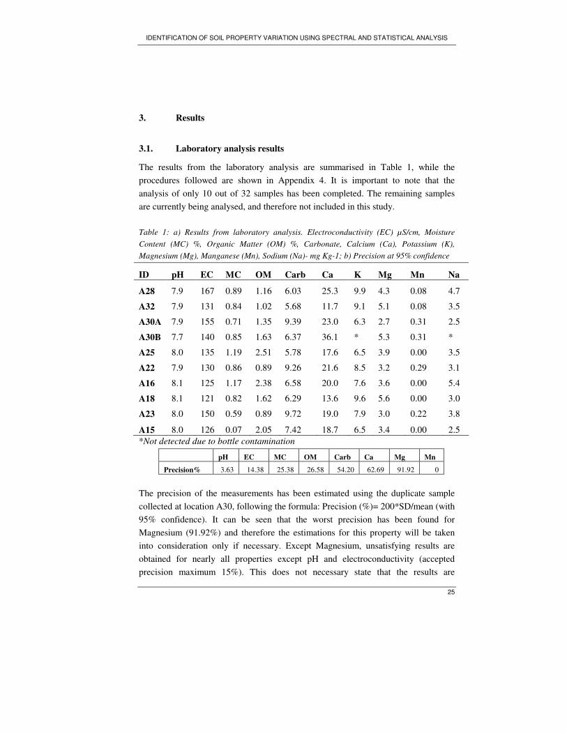
The results from the laboratory analysis are summarised in Table 1, while the
procedures followed are shown in Appendix 4. It is important to note that the
analysis of only 10 out of 32 samples has been completed. The remaining samples
are currently being analysed, and therefore not included in this study.
Table 1: a) Results from laboratory analysis. Electroconductivity (EC) µS/cm, Moisture
Content (MC) %, Organic Matter (OM) %, Carbonate, Calcium (Ca), Potassium (K),
Magnesium (Mg), Manganese (Mn), Sodium (Na)- mg Kg-1; b) Precision at 95% confidence
ID pH EC MC OM Carb Ca K Mg Mn Na
A28 7.9 167 0.89 1.16 6.03 25.3 9.9 4.3 0.08 4.7
A32 7.9 131 0.84 1.02 5.68 11.7 9.1 5.1 0.08 3.5
A30A 7.9 155 0.71 1.35 9.39 23.0 6.3 2.7 0.31 2.5
A30B 7.7 140 0.85 1.63 6.37 36.1 * 5.3 0.31 *
A25 8.0 135 1.19 2.51 5.78 17.6 6.5 3.9 0.00 3.5
A22 7.9 130 0.86 0.89 9.26 21.6 8.5 3.2 0.29 3.1
A16 8.1 125 1.17 2.38 6.58 20.0 7.6 3.6 0.00 5.4
A18 8.1 121 0.82 1.62 6.29 13.6 9.6 5.6 0.00 3.0
A23 8.0 150 0.59 0.89 9.72 19.0 7.9 3.0 0.22 3.8
A15 8.0 126 0.07 2.05 7.42 18.7 6.5 3.4 0.00 2.5
*Not detected due to bottle contamination
pH EC MC OM Carb Ca Mg Mn
Precision% 3.63 14.38 25.38 26.58 54.20 62.69 91.92 0
The precision of the measurements has been estimated using the duplicate sample
collected at location A30, following the formula: Precision (%)= 200*SD/mean (with
95% confidence). It can be seen that the worst precision has been found for
Magnesium (91.92%) and therefore the estimations for this property will be taken
into consideration only if necessary. Except Magnesium, unsatisfying results are
obtained for nearly all properties except pH and electroconductivity (accepted
precision maximum 15%). This does not necessary state that the results are

IDENTIFICATION OF SOIL PROPERTY VARIATION USING SPECTRAL AND STATISTICAL ANALYSIS
26
unreliable since a detection of external contamination at sample A30B have been
reported and therefore the results from the analysis of this sample should not be
considered as determining. Larger dataset would have overcome this problem.
3.2. Spectral and image analysis
3.2.1. Laboratory spectra and CIE diagram
Table 2: Albedo and soil colour analysis
x y Albedo %
A23 0.42 0.38 35.01
A22 0.43 0.38 29.48
A18 0.43 0.38 32.28
A16 0.43 0.38 30.05
A32 0.43 0.38 30.55
A15 0.42 0.38 29.57
A25 0.43 0.38 30.34
A28 0.42 0.38 31.67
A30A 0.43 0.38 31.6
All ten samples, analysed in the laboratory, have been found to be pale brown
according to the standard Munsell colour chart used in the field. Furthermore, as it
can be seen from Figure A7- Appendix 1.1, the variation between the samples is
minimal. All absorption features expected due to moisture seen in 1000nm, 1416nm,
1919nm and 2217nm are present. Slight absorption is also noted at 841nm, which is
a wavelength associated with presence of Iron. The spectral library has also been
converted into image format in terms of performing albedo and soil colour analysis.
The original idea behind this is to remove the soil albedo from the measurements so
that soil colour variation could be noted. When the results from these analyses,
summarised in table 2, are plotted on the same diagram (see Figure A6), it can be
seen that there is limited variation and indeed the identified colour is the same as the
one observed in the field. The albedo varies from 29.48% (at location A22) to
35.02% (at A23).
IDENTIFICATION OF SOIL PROPERTY VARIATION USING SPECTRAL AND STATISTICAL ANALYSIS
27
3.2.2. PLSR on laboratory spectral library
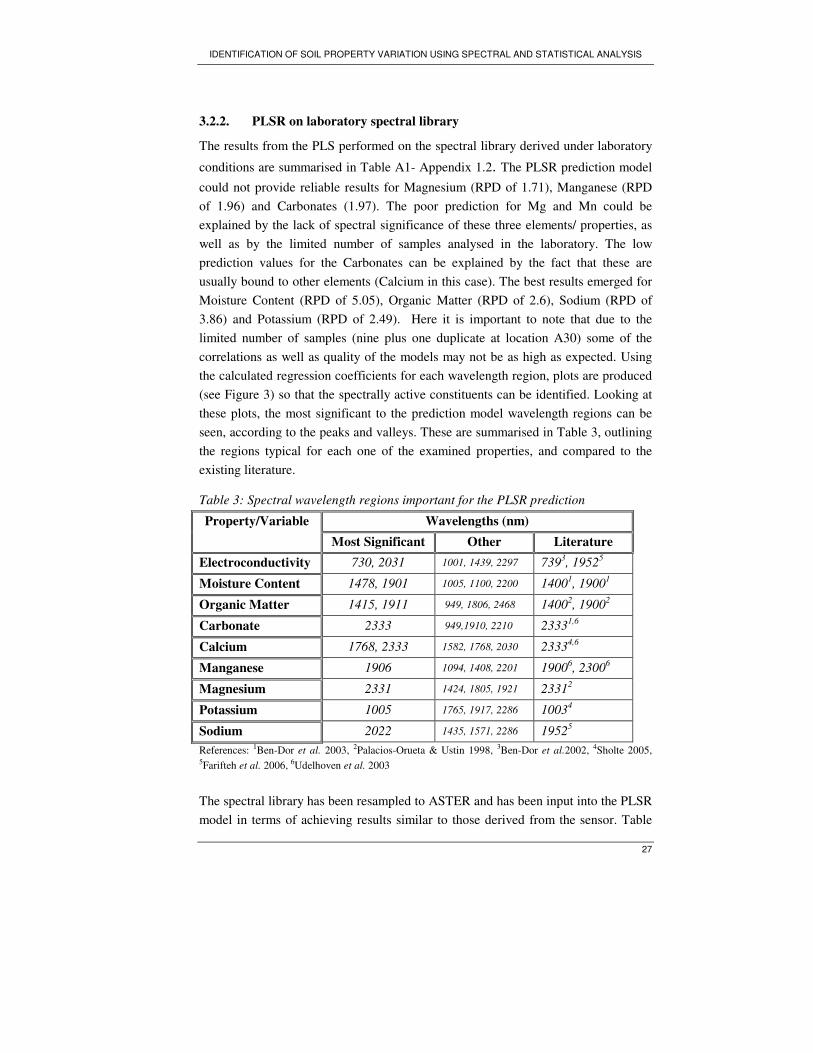
The results from the PLS performed on the spectral library derived under laboratory
conditions are summarised in Table A1- Appendix 1.2. The PLSR prediction model
could not provide reliable results for Magnesium (RPD of 1.71), Manganese (RPD
of 1.96) and Carbonates (1.97). The poor prediction for Mg and Mn could be
explained by the lack of spectral significance of these three elements/ properties, as
well as by the limited number of samples analysed in the laboratory. The low
prediction values for the Carbonates can be explained by the fact that these are
usually bound to other elements (Calcium in this case). The best results emerged for
Moisture Content (RPD of 5.05), Organic Matter (RPD of 2.6), Sodium (RPD of
3.86) and Potassium (RPD of 2.49). Here it is important to note that due to the
limited number of samples (nine plus one duplicate at location A30) some of the
correlations as well as quality of the models may not be as high as expected. Using
the calculated regression coefficients for each wavelength region, plots are produced
(see Figure 3) so that the spectrally active constituents can be identified. Looking at
these plots, the most significant to the prediction model wavelength regions can be
seen, according to the peaks and valleys. These are summarised in Table 3, outlining
the regions typical for each one of the examined properties, and compared to the
existing literature.
Table 3: Spectral wavelength regions important for the PLSR prediction
Wavelengths (nm) Property/Variable
Most Significant Other Literature
Electroconductivity 730, 2031 1001, 1439, 2297 7393, 1952
5
Moisture Content 1478, 1901 1005, 1100, 2200 14001, 1900
1
Organic Matter 1415, 1911 949, 1806, 2468 14002, 1900
2
Carbonate 2333 949,1910, 2210 23331,6
Calcium 1768, 2333 1582, 1768, 2030 23334,6
Manganese 1906 1094, 1408, 2201 19006, 2300
6
Magnesium 2331 1424, 1805, 1921 23312
Potassium 1005 1765, 1917, 2286 10034
Sodium 2022 1435, 1571, 2286 19525
References: 1Ben-Dor et al. 2003, 2Palacios-Orueta & Ustin 1998, 3Ben-Dor et al.2002, 4Sholte 2005, 5Farifteh et al. 2006, 6Udelhoven et al. 2003
The spectral library has been resampled to ASTER and has been input into the PLSR
model in terms of achieving results similar to those derived from the sensor. Table

IDENTIFICATION OF SOIL PROPERTY VARIATION USING SPECTRAL AND STATISTICAL ANALYSIS
28
A2-Appendix 1.2, contains the values used for the assessment of the prediction
models ran on the resampled library. It has been proven to be very good only for
electroconductivity, with highest RPD of 3.79. Good results are obtained for organic
matter, Calcium and Sodium, while in the RPD range between 1.5 and 2 fall
Moisture Content, Potassium, Magnesium and Manganese. The worst results have
been observed for Carbonates, which could be driven by the same factors that affect
this property in the previous PLS analysis. The regression coefficients from these
PLSR analyses were plotted against those from the first set and the results are
displayed on Figure 4. This has been done in terms of outlining peaks and sinks
commonly present on the graphs from the laboratory derived spectra and the
resampled library. The important wavelengths are: moisture content: 2264nm and
2333nm; Carbonates: 1655, and 2165 to 2208; electroconductivity: 805 and
2333nm; organic matter: 2264nm; Manganese: 805 and 2208nm; Calcium: 2208 and
2264nm; Magnesium: 2333nm; Potassium: range between 2165 and 2208nm;
Sodium: 2208 and 2333nm.
3.2.3. Image analysis
3.2.3.1. PLSR for image library
The spectral signatures have been derived per sample, from the ASTER scenes.
These have then been examined in terms of recognising main regions of variation
between the samples as well as common peaks and sinks that coincide with the peaks
and sinks outlined by the previous PLSR analyses (see Figure 5). The PLSR
prediction models have been performed separately for the two images. The results
are summarised in Tables 6 and 7 (Appendix 1.2) for images from 2003 and 2005
respectively. The regression coefficients have been plotted against each other for
identifying the common wavelengths explaining the properties of interest between
the two scenes (Figure 5), and then compared with already identified wavelength
regions from the previous PLS analyses. The model have been proven suitable (very
good) for electroconductivity (RPD of 3.03), while good results obtained for
moisture content, organic matter, and Sodium, result in RPD values greater than 2.
Lower accuracy results are those for Carbonates concentration, Calcium, Potassium,
Manganese and especially Magnesium (RPD of 1.40).
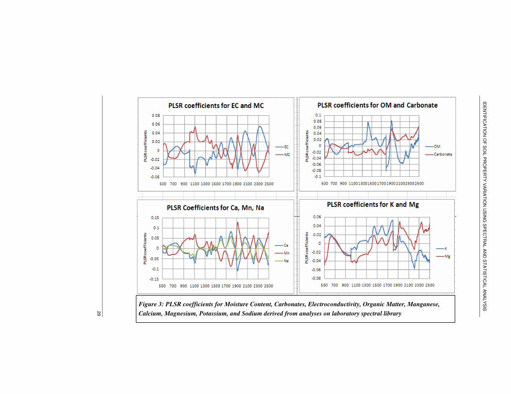
IDE
NT
IFIC
AT
ION
OF
SO
IL P
RO
PE
RT
Y V
AR
IAT
ION
US
ING
SP
EC
TR
AL A
ND
ST
AT
IST
ICA
L A
NA
LY
SIS
29
Figure 3: PLSR coefficients for Moisture Content, Carbonates, Electroconductivity, Organic Matter, Manganese,
Calcium, Magnesium, Potassium, and Sodium derived from analyses on laboratory spectral library

IDE
NT
IFIC
AT
ION
OF
SO
IL P
RO
PE
RT
Y V
AR
IAT
ION
US
ING
SP
EC
TR
AL A
ND
ST
AT
IST
ICA
L A
NA
LY
SIS
30
Figure 4: PLSR coefficients (resampled to ASTER spectral library vs Library derived under laboratory conditions) for Moisture
Content, Carbonates, Electroconductivity, Organic Matter, Manganese, Calcium, Magnesium, Potassium, and Sodium

IDE
NT
IFIC
AT
ION
OF
SO
IL P
RO
PE
RT
Y V
AR
IAT
ION
US
ING
SP
EC
TR
AL A
ND
ST
AT
IST
ICA
L A
NA
LY
SIS
31
Figure 5: PLSR coefficients: ASTER 2003 vs ASTER 2005 for Moisture Content, Carbonates, Electroconductivity,
Organic Matter, Manganese, Calcium, Magnesium, Potassium, and Sodium

IDENTIFICATION OF SOIL PROPERTY VARIATION USING SPECTRAL AND STATISTICAL ANALYSIS
32
When PLSR was run on the library extracted from the ASTER scene (year 2005), the
best results were produced for Magnesium (RPD of 15.37), Calcium (RPD of 4.29),
electroconductivity (RPD of 3.18) and Carbonates concentration (RPD of 2.81). The
prediction models for Manganese and Sodium had RPD of 2.35 and 2.02
respectively, while unsuitable prediction has been done in terms of identifying
Potassium, Organic matter and Moisture Content (RPD<2.0). Figure 5 displays the
common peaks and valleys derived from the PLSR coefficients for the two scenes.
Common wavelengths are: carbonates –1656nm and 2262nm, electroconductivity-
2209nm, Calcium- 1656nm, valley at 2336nm, Magnesium at 2209nm, Potassium-
1656nm and Sodium- 1656nm and 2262nm. The rest of the properties do not
indicate clear common features and therefore the model with more accurate result
has been considered. For Moisture Content and Organic Matter, the model taken into
account is the one developed for spectra extracted from ASTER scene (year 2003),
where the valley at 2336nm have been most clearly defined for both properties. The
same wavelength has been associated with Manganese concentration, however here
the model from ASTER scene (year 2005) has been considered.
3.2.3.2. Classifications
Minimum noise fraction (MNF) is a modified version of the procedure Principle
Component Analysis. It is used to identify and isolate noise (and bands containing it)
in an image. It results in eigenvalues, where the larger the eigenvalue is, the higher
the variance of the data in the transformed band is. If the value is 1, this indicates
that the noise is left in the transformed band (Ramsey, 2006). Ideally, this procedure
should indicate potential end-members in the images. The plots on Figure A4-
Appendix 1.1 show the eigenvalues for each MNF transformed band, for each of the
two ASTER scenes. It can be seen that the MNF bands containing the most noise are
6, 7, 8 and 9 for both images. ISODATA was performed on both ASTER scenes,
selecting 5-10 initial classes, in terms of identifying main homogeneous areas on the
images. The scene dating from year 2003 resulted in 7 classes while after running
ISODATA on the one from 2005, the classes were 9. This could be explained with
the extensive presence of clouds and cloud shadows in the latter scene. An important
issue to note here is that the ISODATA results do not necessarily represent soil types
but most likely represent landcover. The results are displayed on Figure 6a.
The image dating from 2003 has been classified into 9 main soil classes and 1 water
class/no data, while the image from 2005 has two additional classes: clouds and
cloud shadows. The first set of Maximum Likelihood supervised classification
performed included the first nine ASTER bands, and the results are illustrated on

IDENTIFICATION OF SOIL PROPERTY VARIATION USING SPECTRAL AND STATISTICAL ANALYSIS
33
Figure 6b. In terms of improving the accuracy of the classification and at the same
time removing the noise from the scenes, Maximum Likelihood classification has
been applied on the first four Minimum Noise Fraction bands (MNF-ASTER). The
results are displayed in Figure 6c. The full reports of the accuracy assessments,
according to the regions of interest and the reference soil map, as well as the
confusion matrices are included in Appendix 5, while summary of the overall
accuracies of the classifications as well as a list of the most successfully classified
soil types are shown in Table 4.
Table 4: Image classifications overall accuracy, kappa coefficients and most
successfully classified soil types.
Image
classification
Overall
accuracy
Kappa
coefficient
Classes
Maximum
Likelihood-
ASTER 2003
88.05% 0.86 Halomorphic soils, Lithosols,
Water
Maximum
Likelihood-
ASTER 2005
71.34% 0.67 Halomorphic soils, Lithosols,
Fluvial soil, Cloud
MNF- ASTER
2003*
76.12% 0.72 Halomorphic soils, Lithosols
MNF- ASTER
2005*
64.96% 0.59 Halomorphic soils, Fluvial
soils, Clouds, Cloud shadows
*MNF ASTER stands for Maximum Likelihood classification applied on MNF bands 1-4
Another procedure for accuracy assessment has been applied according to the rule
images produced prior to the classifications, and the results for the study area have
been plotted (see Table 5). The results from the two ASTER scenes classified using
all ASTER bands and the first four MNF bands have been combined in terms of
estimating the reliability of the classifications with certain level of confidence. In
general, the overall accuracy of the classifications performed on the image from year
2003 is better than this on the 2005 scene. Explanation behind this is the cloud and
cloud shadow classes, which on its own are classified with good accuracy, however,
they cause problems in terms of the performance of other classes.

IDENTIFICATION OF SOIL PROPERTY VARIATION USING SPECTRAL AND STATISTICAL ANALYSIS
34
Figure 6:ASTER classifications: scene 2003 (left), 2005 (right)a)
ISODATA, b) Maximum Likelihood-all bands; c) MNF bands
a
b
c
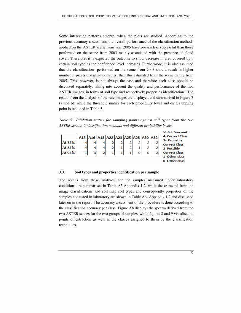
IDENTIFICATION OF SOIL PROPERTY VARIATION USING SPECTRAL AND STATISTICAL ANALYSIS
35
Some interesting patterns emerge, when the plots are studied. According to the
previous accuracy assessment, the overall performance of the classification methods
applied on the ASTER scene from year 2005 have proven less successful than those
performed on the scene from 2003 mainly associated with the presence of cloud
cover. Therefore, it is expected the outcome to show decrease in area covered by a
certain soil type as the confidence level increases. Furthermore, it is also assumed
that the classifications performed on the scene from 2003 should result in higher
number if pixels classified correctly, than this estimated from the scene dating from
2005. This, however, is not always the case and therefore each class should be
discussed separately, taking into account the quality and performance of the two
ASTER images, in terms of soil type and respectively properties identification. The
results from the analysis of the rule images are displayed and summarised in Figure 7
(a and b), while the threshold matrix for each probability level and each sampling
point is included in Table 5.
Table 5: Validation matrix for sampling points against soil types from the two
ASTER scenes, 2 classification methods and different probability levels
3.3. Soil types and properties identification per sample
The results from these analyses, for the samples measured under laboratory
conditions are summarised in Table A5-Appendix 1.2, while the extracted from the
image classifications and soil map soil types and consequently properties of the
samples not tested in laboratory are shown in Table A6- Appendix 1.2 and discussed
later on in the report. The accuracy assessment of the procedure is done according to
the classification accuracy per class. Figure A8 displays the spectra derived from the
two ASTER scenes for the two groups of samples, while figures 8 and 9 visualise the
points of extraction as well as the classes assigned to them by the classification
techniques.

IDENTIFICATION OF SOIL PROPERTY VARIATION USING SPECTRAL AND STATISTICAL ANALYSIS
36
Figure 7: Soil types coverage defined by classification techniques at
confidence levels 75%, 85% and 95%
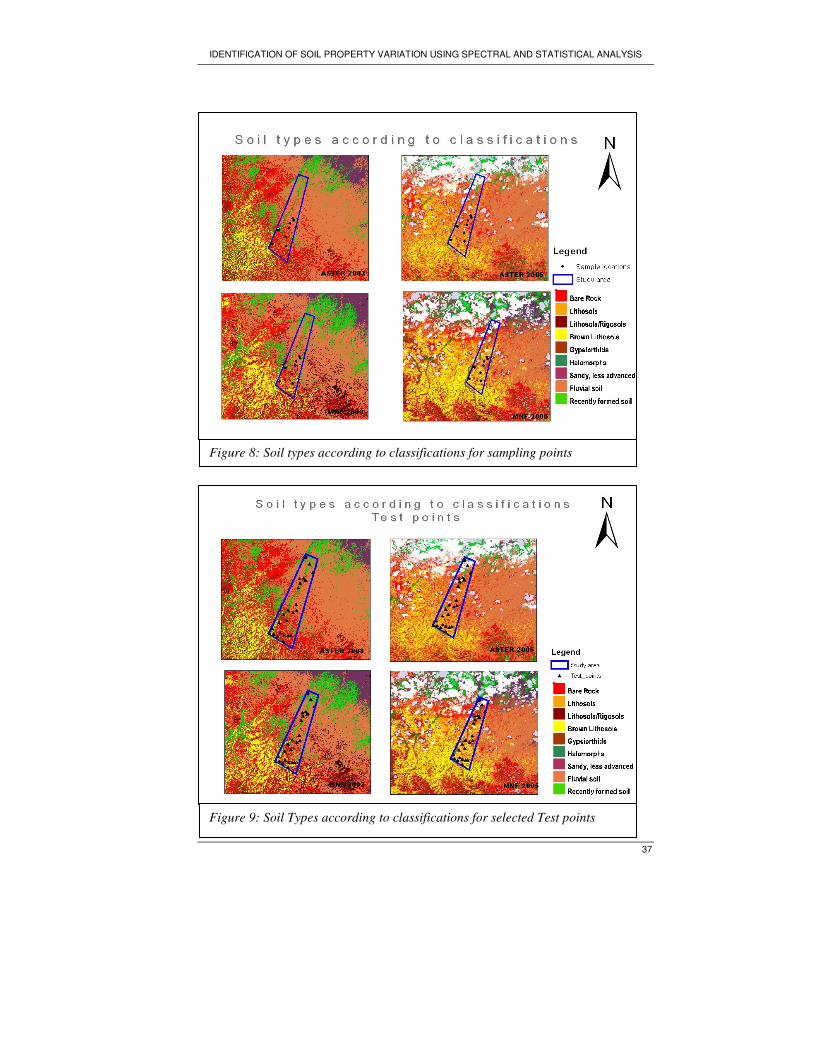
IDENTIFICATION OF SOIL PROPERTY VARIATION USING SPECTRAL AND STATISTICAL ANALYSIS
37
Figure 8: Soil types according to classifications for sampling points
Figure 9: Soil Types according to classifications for selected Test points


IDENTIFICATION OF SOIL PROPERTY VARIATION USING SPECTRAL AND STATISTICAL ANALYSIS
39
4. Discussion
4.1. Spectral library analysis
In this part of the discussion, attention has been paid on the soil colour and albedo
estimates. As it has been determined so far, the difference between the analysed
samples in respect to these two soil characteristics is minimal. However, some
correlations are identified, between these two and the rest of the measured properties.
Correlation analyses have been done so that the variation in albedo, derived from the
CIE diagram and the soil colour analysis, is explained. The results from this clearly
showed that the most significant factor in this case is the electroconductivity (R2
0.78). Even though the electroconductivity has not been found to be the main force
behind any differences in soil albedo, the observations can be explained by the high
salts content associated with the soil types, when compared with the soil maps
described earlier. Correlations of 0.42 and 0.47 have been estimated between the
albedo and organic matter and pH respectively. It has been noted by Post et al.
(2000), that this sort of relationship between soil colour (soil reflectance) and
organic matter is obtained when soils are collected from an extensive geographic
area or the soils have a wide range of soil properties. The small study area as well as
the limited number of sampling units, explain the weak correlation, however, it is
important to acknowledge the fact that the number of tested properties is relatively
small and there might be other, significant ones, not considered in the study.
Interestingly, moisture content, the factor identified in the literature (Post et al.,
2000) as one of the most important when it comes to albedo estimates, has not been
found to be correlated or significant (R2 0.27). This can be explained mainly by the
limited presence of moisture in the soil, due to the geographic location of the study
area as well as the season of sampling.
Overall, it can be seen that the soil colour and albedo can play a significant role if
there is wider dataset and greater variation between the estimated values. However,
what was established so far serves as a base for choice of normalisation technique in
the following PLSR analysis. The lack of significant difference between the albedo
estimates determined the removal of this characteristic from further analysis

IDENTIFICATION OF SOIL PROPERTY VARIATION USING SPECTRAL AND STATISTICAL ANALYSIS
40
4.2. Partial Least Squared Regression models
PLSR modelling has been applied extensively by many (Viscarra Rossel, 2006;
Scholte, 2005, Lee et al., 2003, Udelhoven et al., 2003), in terms of identifying the
significance of some bands/wavelengths in soil properties identification. Diffuse
reflectance has proven itself as a successful screening method to characterise soil
chemical properties (Ben-Dor & Banin, 1995). It has been made clear that the PLSR
prediction model identifies more significant wavelengths than what can be seen from
the soil spectral signatures alone. It is important to note, however, that many
chemical compounds show overlapping bands in the SWIR region. According to
Scholte (2005), the regions between 1115-1150 nm, 1345- 1417 and 1820-1932nm
should be left out of the discussion because they are associated with major water
vapour absorption areas. Furthermore, a great limitation is the fact that soil chemical
properties, as outlined by Udelhoven et al. (2003), are not independent from each
other. Variables, not studied and therefore not identified, play a major role in
outlining correlation, causing indirect effects on the results. Another limitation is the
bound compounds such as Calcium Carbonate (CaCO3). The PLSR model indirectly
estimates Calcium since in most cases the Carbonate group is stronger in terms of
estimating the values for the model, or in other words, the form of the compounds is
crucial. A constraint, which should not be excluded, is the limited number of
laboratory measurements integrated into the model.
Udelhoven et al. (2003) tested the feasibility of the analysis of certain chemical
properties using PLSR and diffuse reflectance spectrometry. They indicated that the
indirect correlations are those that prevent PLSR models from being applied to other
areas where the correlation structure among the soil constituents significantly differs.
In theory, a possible up-scaling requires the consideration of factors such as the
atmospheric transmission path and larger spectrally mixed footprints. Therefore, the
correlations of certain properties with the spectra, found in the present study, have
been compared with those estimated by Udelhoven et al.( 2003), Farifteh et al.
(2006), and Lee et al. (2003), in terms of testing the overall applicability of the
PLSR technique. Conclusions can be drawn only about the correlations regarding the
spectral library derived in the laboratory due to the fact that no PLSR analyses have
been done on the spectra from satellite imagery in the above three studies. A
correlation of 0.8 between the spectra and electroconductivity (EC) has been found
by Farifteh et al. (2006), which concurs with the R2 estimated for EC by the PLSR
model for the soil spectral library produced in the laboratory. Much better estimates
have been found when the library is resampled to ASTER (R2 of 0.92) and the

IDENTIFICATION OF SOIL PROPERTY VARIATION USING SPECTRAL AND STATISTICAL ANALYSIS
41
ASTER derived spectral library for the same locations (R2 of 0.88). This could be
explained by the fact that due to the poorer spectral resolution of the scene, the
spectral variations at the image level are much smaller (Farifteh et al. 2006).
Furthermore, within an area of one ASTER pixel, soil moisture, soil type and
reflectance of other scene components affect the spectral variation and therefore
result in an error in the prediction model, even though the RPD and RMSE values do
not indicate this. Lee et al. (2003), performed PLSR analyses on Ca, OM, Mg, K and
P in terms of finding more accurate and advance solution to farm land management.
Generally, however, their findings in terms of accuracy of the PLSR models are
limited. The strongest correlation found between spectra and soil properties is for
Calcium (0.88). The rest performed poorly, which the authors explain by the
complex interaction between soil colour and soil properties.
The correlation found between the spectra and moisture content, has been estimated
by all, and this coincides with the reported results from this study for the laboratory
spectral library analyses (R2 of 0.95). Much weaker correlation have been estimated
for the resampled library as well as for the library derived from ASTER (R2 of 0.63
and 0.73 respectively). The study by Udelhoven et al. (2003) looked at the
correlations between Calcium, Organic Carbon, Manganese and Potassium. The
Calcium correlation with the spectra established in their work (R2 of 0.94) has been
found to be the same as what was estimated in the current report; however, this value
is derived from the analyses of the library from the ASTER scenes. When it comes to
the correlation between the spectra from the laboratory analyses and the Calcium
concentration, the R2 estimate is 0.74. There could be many reasons behind this
including the small sample size, relatively different concentrations of Ca found
within the two studies, climate and atmospheric condition differences. Another
disagreement has been recognised in terms of Potassium even though strong
correlation was found only between the property and the spectra from the library
produced from the spectroscopy measurements obtained in the laboratory (R2 of
0.82). Although, Udelhoven et al. (2003) state that lower value than R2
of 0.5 has
been produced from the PLSR analysis for Potassium, which is the case of the
analysis on the resampled to ASTER library and the derived from ASTER scenes
library. Considering the Manganese concentrations, perfect match between the
derived R2 values in the current study from the laboratory spectral library and the
Udelhoven et al. (2003) team, has been found (R2 of 0.71). Lower correlations were
observed between this property and the spectra included in the resampled and
ASTER spectral libraries. Overall, the highest correlations (R2 higher than 0.9)
derived from the laboratory spectra as outlined in earlier chapters, are those of

IDENTIFICATION OF SOIL PROPERTY VARIATION USING SPECTRAL AND STATISTICAL ANALYSIS
42
Moisture Content and Sodium (found at 1100nm and 1760nm respectively), from the
resampled library is only the Electroconductivity (at 2333nm), and from ASTER
scenes spectra- Magnesium, Electroconductivity and Calcium (at 2209nm for the
first two and 1656nm for Ca). In terms of assessing if these correlations correspond
to the spectral regions typical for the properties, five sampling locations were used
(see Figure A9- Appendix 1.2). These locations were associated with the highest
concentrations estimated in the laboratory for Moisture Content, Electroconductivity,
Sodium, Calcium and Magnesium- A16, A18, A25, A28 and A30.
The specific wavelengths associated with the properties giving highest correlation
are illustrated on the Figure A9. The first issue that emerges is the missing
absorption feature at 1100nm associated with moisture content. It can be seen
slightly on the spectral response from sample A25, which is also the one with the
highest laboratory estimate. This weak absorption band, according to Baumgardner
et al. (1985) corresponds to the absorption bands observed in transmission spectra of
water of a few millimetres thickness. It is assigned in terms of water vibrations, with
additional combination of librations of the water molecule in the 1770 nm band,
which is also not present. The most reasonable explanation behind this as well as the
determination of the strong correlation by the PLSR model is not only the small
variation between all observations, but also the limited presence of moisture content
(highest of 1.19%) for all soil samples. The absorption feature expected to explain
the Sodium concentrations is present and distinctive for the samples with the highest
correlation estimated by the PLSR model. Obviously, if the spectral library is
considered on its own, without combining the results from all PLSR models, there
are other important wavebands associated with Moisture Content, and picked by the
PLSR model including 1450nm and 1950nm.
When the created spectral library is resampled, as mentioned earlier, only the
electroconductivity showed coefficient of determination higher than 0.9. It was
determined by the model that this property corresponds to 2333nm wavelength and
the absorption feature is present for all samples having high levels of it. On the other
hand, interesting observation is the matching wavelength typical for Magnesium and
Electroconductivity (2209nm) identified by the PLSR model performed on the
library extracted from the ASTER scenes. According to Farifteh et al., 2006, the
accurate prediction of electroconductivity could be used to predict Mg containing
salts. The lack of correlation observed from the laboratory analysis (R2 of 0.33),
between the two properties, suggests that there are other factors that affect the
spectra and the prediction model for ASTER imagery. Mainly, however, the

IDENTIFICATION OF SOIL PROPERTY VARIATION USING SPECTRAL AND STATISTICAL ANALYSIS
43
insufficient number of samples prevents from determining whether the error occurs
at correlation estimation level, or ASTER scene level. In the case of Calcium, the
corresponding waveband, determined by the PLSR model to be 1656nm, has been
explored in terms of identifying the reliability of the prediction. The deepest
absorption feature has been observed for sample A30, even though the location has
been identified with having the second highest Ca concentration. However, as
clarified earlier, the PLSR model takes into account the Carbonate group that acts as
the stronger property influencing the spectra at the same spectral region, despite the
fact that strong correlation was not identified by the model for this group.
The results from the PLSR analysis in this report illustrate how from a large number
of significant for the prediction model wavelengths per property, extracted from the
laboratory spectral library, the spectral regions of importance have been reduced to
maximum of two or in some cases none common wavelengths, when ASTER
spectral library is studied. The results also show that there are many factors that
should be taken into account when soil samples analysed in laboratory are linked to
satellite images. The most important of all is the change in spectral resolution
ultimately resulting in the removal of the weaker absorption features. Furthermore,
the wavelengths at 2208 and 2333nm have been observed to be the most important
for the PLS prediction modelling, including most of the properties (Moisture
Content, Electroconductivity, Organic Matter, Manganese, Calcium, Potassium and
Sodium). The wavebands identified as the most important for the determination of
the soil properties by the PLSR models can be explained by the occurrence of certain
absorption features or general observations that determine the soil reflectance
spectra. These include the decrease of soil reflectance between 400 and 2500nm as
the organic matter content increases, the two very strong absorptions at 1400 and
2200 nm associated with typical kaolinite reflectance with lack of appreciable bound
water, resulting in only a weak band at 1900nm (Baumgardner et al. 1985). The
presence of kaolinite is also associated with a small amount of ferrous ion resulting
in the slight absorption at 1011nm. Furthermore, the Aridisols, generally high in
soluble salts, determine the high average reflectance observed between 520 and
900nm, which is also confirmed by Baumgardner et al. (1985).
A more accurate results could be observed if the area of sampling is classified
according to main geological features and the PLS models are calibrated with these
results instead of with a global model. To do this, however, as shown with this study
and further proven by Udelhoven et al. (2003), not only a larger data set is required
in terms of producing a stable model, but also water accumulation rate as well as

IDENTIFICATION OF SOIL PROPERTY VARIATION USING SPECTRAL AND STATISTICAL ANALYSIS
44
other properties influencing the measured, should be taken into consideration.
Further work can also look into a way of sampling one pixel (30 by 30 meters in the
SWIR region) and exclude noise caused by properties that are not of interest.
Generally, the PLSR procedure was applied to the spectra in terms of identifying the
most important for the properties prediction and identification wavelength regions.
Furthermore, the results have been used as a link between the laboratory spectra and
the spectra derived from the two ASTER scenes (discussed in the next section). The
purpose if this is to estimate or predict, as accurately as possible, the level of
properties concentration.
4.3. ASTER scenes analysis
4.3.1. Spectral profiles per sample
According to Figure A6, the feature at 2167nm observed at sampling locations A30
and A32 in year 2003 and at all profiles derived from the scene from year 2005,
could be associated with Potassium concentrations. It is interesting to examine the
behaviour of the spectra at 1656nm observed for all location in year 2003 and deep
absorption at the same wavelength found for all locations in year 2005. This
wavelength is also associated with abundance of carbonate groups, which could be
explained by the limestone presence (CaCO3), Calcium and higher moisture content.
Furthermore, it can be seen that variation between locations is mainly found between
2209 and 2336nm for ASTER scene from 2003 and 2167 and 2262nm for ASTER
scene from 2005. It can also be observed that there are three wavelengths common
for both scenes: 660nm, 2209nm and 2262nm. Referring to the PLS analysis these
three features are associated with Calcium and Magnesium content characteristic for
the type of soil in the region. The variation within the above wavelength regions has
been compared with the actual concentrations of the properties, measured in the
laboratory.
The negative correlation observed between Calcium and Magnesium concentrations
(R2 of -0.67), can be also noted looking at the derived spectral profiles. Interestingly,
however, the fluvial soils with Ca/Mg encrusting do not have defined ratio, typical
for all sampling points. This varies from 8.5:1 at A30 associated with Magnesium
deficiency (Department of Natural Resources, 2007) to 2.3:1 at A32. According to
the soil map of the area, the soil samples at locations A32, A18 and A15 are the three
not associated with Ca/Mg encrusting, which could explain the small ratio between
the elements. Some unexpected findings have been related to 2203nm wavelength,
typical for Calcium rich soils. The pattern that should emerge in terms of absorption

IDENTIFICATION OF SOIL PROPERTY VARIATION USING SPECTRAL AND STATISTICAL ANALYSIS
45
values does not follow the pattern established from the laboratory results. In other
words, the soil samples showing the highest concentrations of Calcium do not appear
on the spectral response as having the strongest absorption on any of the ASTER
scenes. This could be explained by the undefined form of Calcium in the samples. In
terms of Magnesium concentrations, the spectra at 661nm behave as expected, with
some exceptions at location A23 and A30. It is also very important to note that the
characteristics of the soil types, especially when it comes to soil properties, apply to
the soil horizon, while the samples have been collected from the top 10cm in terms
of appropriate comparison with the results from the satellite imagery.
The spectra derived from the ASTER scenes was not only included in the PLSR
analyses, but also it was used as a determining for the soil composition factor. The
observed differences between the laboratory spectra and these measured on the
images are caused by the decrease in spectral resolution (as discussed earlier). The
strong absorption features identified by the PLSR analyses were studied and
implemented later in the soil properties identification per sampling point.
4.3.2. Classifications
Looking at the Table 4 it can be seen that the soil types most successfully classified
by all classification techniques are the Halomorphic soils and the Lithosols. As
mentioned earlier in the report both types of soils are typically very pale brownish
soils rich in soluble salts. The former are typical for regions close to saline water
bodies while the latter are one of the most commonly found soils in Tunisia and most
of the arid and semi-arid regions. Moreover, the region South-West of the study area
is known as the largest salt marsh in Sahara desert- Chott el Djerid. The problem
associated with this is the high reflectance occurring due to the nature of the salt
marsh. On ASTER imagery this region appears completely white causing problems
in identifying soils or any other characteristics of the surrounding areas. A main
limitation of all classifications is the fact that the regions of interest (training and
testing sites) have been selected according to a soil map dating from 1973. Knowing
the high rate of erosion and desertification in the area, as well as the lack of
sufficient field data for validation, the main challenge behind the image classification
description is to identify whether the difference that appears is due to change, image
noise or inaccurate classification. Furthermore, due to the cloud formation over some
parts of the image from year 2005, the information is limited for some of the soil
classes. Nevertheless, similarities in the classifications as well as patterns do emerge.
In terms of the Halomorphic soils, their location and extent corresponds to what is
expected as an output from the classifications. There is a problem occurring due to

IDENTIFICATION OF SOIL PROPERTY VARIATION USING SPECTRAL AND STATISTICAL ANALYSIS
46
the extensive cloud cover present on the scene from 2005, however this did not affect
the classification of the Halomorphic soils to a great extent. The Lithosols, Lithosolic
brown and the mixed Lithosols/Regosols classes are more problematic, although the
estimated accuracies for these classes are found to be over 87%. Here, the need of
validation field data is essential, since the rate with which the salt marsh close to the
study area increases and varies over the years, driven by many complex climatic
conditions. However, it could be expected that the change appearing between the two
classifications is not entirely due to noise and faults in the second scene, but also due
to actual change. Further contribution to this statement has the fact that the three
classes are similar in nature (all of them belonging to the group of Lithosols) and
therefore more difficult to differentiate. In terms of the class that includes bare rock,
the change could be explained by increase in the soil erosion rate. The fluvial soils,
on the other hand, characterised by their specific location (near rivers) and the
presence of relatively large stones and sediment deposits, are more difficult to
identified with simple classification technique such as Maximum Likelihood, even
when the noise is removed from the scenes. Moreover, the irregular precipitation and
the extensive evaporation result in the formation of gypsum. The fact that the
gypsum is in sandy form can be an indicator for easy wind transportation of particles.
However, the poor quality of the ASTER scene from 2005, especially in the regions
where gypsum is present, prevents from drawing any conclusions about change or
pattern. To identify the regions on the ASTER scenes, which have been misclassified
due to noise, accuracy assessment have been performed comparing the classification
on the nine ASTER bands with the ones done on the MNF bands 1- 4. The
misclassification mainly applies to the bare rock class, which phenomenon could be
explained by possible difference in rock types not identified due the unavailability of
geological maps for the region. The error, discussed earlier, explaining the
classification of the Lithosols, Brown Lithosols and Lithosols/Regosols classes is
illustrated in Figure A10-Appendix 1.2. The least error has been indicated for the
Halomorphic soil type, which was noted after the performance of accuracy
assessment according to the regions of interest earlier in the report.
From the analyses of the Rule images, it can be seen that there are two dominating
classes in the area and these are the ‘Brown Lithosols’ and ‘Fluvial soil’. Maximum
Likelihood classification including all ASTER bands and the same classification on
the first four Minimum Noise Fraction bands, performed on the ASTER scene from
year 2005 resulted in higher number of accurately classified pixels for these
dominant classes, despite the fact that the overall accuracy for this scene is lower.
The classifications performed on the scene from 2003, on the other hand, resulted in

IDENTIFICATION OF SOIL PROPERTY VARIATION USING SPECTRAL AND STATISTICAL ANALYSIS
47
more pixels classified correctly at 95% level of confidence for the ‘Bare rock’ and
‘Gypsiorthids’ classes (see Figure A1-Appendix 1.2). There are many reasons behind
this, one of them being the equalisation of the image brightness between the two
scenes (by histogram matching) prior to the classifications, which consequently
resulted in removing the finer detail caused by the albedo from the scene from year
2005, and therefore affecting the classes less present at the scene. Another
explanation is the atmospheric conditions differing for both scenes. Since the
FLAASH algorithm that takes into account the time of acquisition as well as
geographic location of the image did not show satisfactory results, factors such as
atmospheric transmittance, combined with the spectral mixing, could cause reduction
of the accuracy and performance of the scenes.
The expected phenomenon related to the reduction of the number of pixels classified
correctly with the increase in confidence level, can be seen for all classes on both
scenes and classifications. A main limitation is the fact that the four soil types
included in this discussion, tend to have similar spectral response due to the issues
emerging from particle size, soil crusting formation, smaller variation in soil colour
and properties, all discussed earlier. Thus, the results mainly show high spectral
mixing creating a problem in terms of accurately assigning the pixel to the
appropriate class. To overcome this, the results from the two scenes and the
classification of the different ASTER and MNF bands were compared and combined.
Three probability levels were selected (75%, 85% and 95% confidence), and the 9
validation points were tested against the pixel probability. The procedure resulted in
the creation of a validation matrix (Table 5), illustrating the assigning of classes to
the pixels containing the points at each probability level. The results are then
compared with the actual concentrations of the properties of interest measured in the
laboratory, and a conclusion is drawn for each point. A great drawback of the
procedure is the limited number of validation points, which prevents from
interpolating the accuracy results beyond the tested pixels.
As it can be expected, at the lowest confidence level of 75%, more pixels are
assigned to the same class on both scenes by the different classifications, than at
higher level. Referring to Table 5, it can be seen that three of the validation pixels
were assigned the correct soil class not only with 75 but also 85% confidence- A15,
A16 and A18: fluvial soil. With 95% confidence, however, A15 is assigned to a
different from these 4 classes, or it is not classified. The classification of the first
four MNF bands of the ASTER image from 2003 did not allocate the pixel
containing A16 to any of the four classes of interest, while as ‘Fluvial soil’ it was

IDENTIFICATION OF SOIL PROPERTY VARIATION USING SPECTRAL AND STATISTICAL ANALYSIS
48
recognised by the rest of the classification outputs. A18 was classified as ‘Fluvial
soil’ by the two ASTER scenes, but only when Maximum Likelihood algorithm was
applied on all ASTER bands. The results from this analysis in regards to the rest of
the validation samples were accepted. Evidently moving closer to the border
between two soil types, the number of mixed pixels increases. This is especially the
case with the locations A22, A25 and A32, where the mixing of soil properties
causes the problem associated with the classification of these pixels. Therefore, these
are allocated to class ‘possibly correctly classified’ on Table 5. At 95% confidence,
two locations have not been allocated to any of the classes of interest by any of the
classification techniques- A28 and A30. Reasonable explanations for this could be
many including the slightly higher percentage albedo characteristic for the two
locations (as well as for location A25), preventing the classification algorithm to
assign accurately (or at all) these pixels to a soil class typical for the other locations.
The removal of the albedo from the laboratory spectra prior to the PLSR modelling
seemed to have overcome the problem. Consequently removing it from the image
spectra could improve the accuracy of the technique. A combination of the results
from the classifications performed using different ASTER and MNF bands on both
scenes, provides a reasonable validation for area where not much is known, and not
many validation points are tested. To further improve the accuracy assessment from
Rule images, the correctly classified pixels per class from each of the performed
analyses, can be overlaid and only the ones that coincide on both scenes and both
classification techniques, for particular confidence level, should be taken into
account. In this way, the limited number of validation points can be overcome by
comparing spectral responses from correctly classified pixels with the rest of the
pixels.
Interesting discussion emerges from the issue related to band selection and expected
spectral response for the soil types and consequently the soil properties. As already
established, a number of properties have been associated with the same waveband
from the SWIR region of ASTER by the PLSR models interest (MC, EC, Mg, Na- at
2333nm, Carbonates, EC, Mn, K at 2208nm, etc.). Although this is the case, as
discussed earlier, properties such as EC, OM, salts and sand content affect the whole
spectrum by decreasing or increasing the overall spectral reflectance. Therefore, the
selection of specific ASTER bands prior to the classifications in terms of reducing
the noise from outside factors, is a challenge. A further work can emphasise on
certain bands or band ratios typical for only one of the properties and repeat the
procedure accordingly for the rest of the properties of interest. Unfortunately due to

IDENTIFICATION OF SOIL PROPERTY VARIATION USING SPECTRAL AND STATISTICAL ANALYSIS
49
limited time available for the completion of the current study, this approach could
not be implemented.
The image classifications were performed so that the soil types within the area of
interest are identified. Due to the limited dataset, sufficient information about the soil
properties was not acquired and therefore the determination of the soil types by the
classifications was used as a reference to the expected soil properties. The results
from the classification techniques are referred to in more detailed in the next section
of the discussion, where soil properties identification has been done per sampling
point taking into account the results from the geochemical laboratory analysis, PLSR
models as well as the derived spectra in the laboratory and from the ASTER scenes.
4.4. Soil types identification within the study area
Looking at Table A5-Appendix 1.2, it can be seen that for some points the
classification results coincide with what is displayed on the soil map, while for other
points this is not the case (illustrated on Figure 8). To identify the correct soil type
of the samples the properties organic matter (OM), electroconductivity (EC) and
Calcium (Ca), Magnesium (Mg), Sodium (Na) and Potassium (K) concentrations are
considered. In this respect, literature has been consulted in terms of identifying the
characteristics of the soil types falling within the study area according to the
classifications as well as the reference soil map-Ministry of Agriculture, 1973. The
same procedure is applied on the 25 samples which have not been analysed in the
laboratory. It is important to note that all the arguments and assumptions used in this
section apply only to the soil surface (0-10cm depth). The characteristics of the soil
profile related to different soil types, have not been studied and therefore may result
in misinterpretation.
With the CIE analysis and the field observations (see Appendix 2) it was shown that
the soil colour at all of these locations is the same as the 9 previously tested.
Considering the small study area and the small variation between the tested samples,
it can be assumed that the additional set have similar spectra and properties and
therefore the PLSR models could be used in terms of interpreting the spectra derived
from the images, if required.
The findings show that the large sediment particles, distinctive for fluvial soils, have
a strong influence on the spectral response. This, therefore, explains the fact that at
locations A16 and A28, the soil type (Fluvial soil) has been allocated most
accurately by all classifications. Moreover, locations A16, as well as A22, are a clear
illustration of the fact that clear borders between soil types do not exist, and the scale

IDENTIFICATION OF SOIL PROPERTY VARIATION USING SPECTRAL AND STATISTICAL ANALYSIS
50
of the reference soil map does influence the accuracy of the results. The grain size
can cause confusion not only in the case of fluvial soils identification. A good
example for this is location A25, where the classifications of the image from year
2005 recognise the soil type as fluvial soil (match with soil map), while the scenes
from 2003 indicate bare rock. These could not only be related to the limited quality
of the image from year 2005, but also to the stage of formation of the Calci-
Magnesium crust, typical for the region. To identify the main reason behind this,
laboratory data for the actual concentrations of Calcium and Magnesium, from both
years, could have played an important role. Furthermore, it is generally known that
the region is rich on limestone (CaCO3); however, more detailed investigation of the
geology of the region is useful in terms of identifying the properties of the bare
rocks.
When the laboratory analyses are taken into account, the values for Calcium and
Magnesium observed at this sampling point are almost identical to those observed at
A16 (fluvial soil with Ca/Mg encrusting). The spectral curve also follows the same
pattern with difference of 0.01 in reflectance (SWIR region). Looking at the spectra
derived under laboratory conditions (Figure A7), a feature can be observed at
2215nm, which does not appear for any of the other sampling locations. This
wavelength is associated with moisture content according to the PLSR analysis and
the finding corresponds to the laboratory measurements (A16 has the highest
percentage moisture content). Interestingly, referring to the spectra derived from the
ASTER scenes (see figure A8), location A16 is not characterised by a feature at
661nm, which, according to the PLSR analyses, should indicate small Magnesium
concentrations. This could indicate that due to the specific location of this point (on
the border between fluvial soils with Ca/Mg encrusting and Brown lithosols), mixing
of some properties may have occurred. The same problem arises at location A32,
however here the ASTER scene from year 2005 also indicates different class- bare
rock. An explanation behind this is the fact that due to erosion and relatively thin
layer of soil, larger sediment material may have been present. Not as clear is the fact
that the classification performed on the first four MNF bands launches different from
the reference map results. Both scenes identify the soil class as brown lithosols,
while the map indicates fluvial soils with Calcium-Magnesium encrusting. Here,
comparison between the laboratory results at location A16 (fluvial soil), A22 (brown
lithosols) and A32 has been done. A great difference is observed between the values
estimated for Calcium and Magnesium between A32 and the other two reference
locations, most probably due to the mixed nature of soils at location A22, as
explained earlier. Similarities have been observed between A22 and A32 in terms of

IDENTIFICATION OF SOIL PROPERTY VARIATION USING SPECTRAL AND STATISTICAL ANALYSIS
51
electroconductivity, moisture content, organic matter, potassium and sodium
determined in the laboratory. Moreover, the spectra derived from the ASTER scenes
are for the two locations, are characterised by much higher overall reflectance
values. The reason behind this could be higher sand content or presence of different
salts, not included in the present study. Therefore, it could be concluded that the
difference between the predicted by the MNF classifications and the reference soil
map occurs due to the scale of the map, inaccuracy of the map, problems with
georeferencing or undefined soil constituents. Referring to the probability levels
associated with the classifications accuracies, with 95% confidence only location
A16 falls into ‘probably’ classified correctly group, while A18 and A32 are the
‘possibly’ classified correctly locations. Therefore, a larger dataset is crucial in terms
of accurate prediction of the soil types and consequently soil properties associated
with them.
Nevertheless, the possibility of observing landcover change between the two years is
not excluded, considering the high erosion rates as well as the lack of validation data.
At location A23 bare rock is identified by ASTER scene from 2003, while image
from 2005 recognises the soil type as Brown Lithosols. The problem here, however,
is mainly the fact that the soil reference map shows fluvial soil as characteristic for
the location. To find out whether fluvial soils can be mistaken for bare rock on
ASTER imagery, or this misclassification is simply a result of a limitation of the
technique; the properties estimated in the laboratory, as well as the results from the
PLSR analyses and the derived spectra have been compared for the two locations
recognised as fluvial soils on the soil map, with location A16 correctly classified on
all scenes. Limited difference, mainly associated with brightness, has been observed
in the SWIR region of the spectra, for sample locations A16 and A25. In contrast,
location A23 is defined not only by the highest reflectance values, but also by much
more defined feature at 2262nm related to Calcium carbonate presence (PLSR
analyses section 3.2.3.1.). Furthermore, great similarities can be observed between
the estimated laboratory concentrations at location A25 and those at A16 in terms of
electroconductivity, moisture content, organic matter, carbonates, Calcium,
Magnesium and Manganese, while between A16 and A23 resemblance occurs only
for Calcium, Potassium and Magnesium (refer to table 1, section 3.1). Therefore it
could be concluded that the soil types at A16 and A25 are more likely to be the
same, but to defer from the one at location A23. It is possible, however, that the
presence of Calci-Magnesium encrusting has been very strong in year 2003, however
no validation data is available from this year. Moreover, the possibility of an error on
soil map level is also considered.

IDENTIFICATION OF SOIL PROPERTY VARIATION USING SPECTRAL AND STATISTICAL ANALYSIS
52
Looking at locations characterised by Brown Lithosols soil type and considering that
this soils are mainly found at steep slopes areas with risk of severe erosion (FAO,
2006), the effect from elevation difference should be considered. Referring to the
digital elevation model extracted from the ASTER scenes, interesting observations
can be seen for locations A22 and A23. The uncertainty that is noted in terms of
identifying the soil type from the ASTER scene (year 2003), by supervised
classification on ASTER bands 1-9, can be related to the shadow due to elevation.
Before the noise is removed with Minimum Noise Fraction (MNF), the soil is
recognised as Gypsiorthids, characterised by high gypsum content and appearing
dark on satellite imagery. PLSR and laboratory analyses of gypsum could overcome
the problem. If this is not considered, the soil type at location A22 is classified
correctly according to the soil map.
Before moving on to the testing sites not measured in the laboratory, selected in
terms of assessing performance and applicability of the technique, it is important to
refer to the probability levels associated with the correctly classified pixels. Taking
into account the small number of validation points, as well as the relatively small
amount of correctly classified pixels with 95% confidence, the properties prediction
done on the samples not tested in the laboratory is only hypothetical and cannot be
considered statistically accurate. Soil material collection and laboratory analysis
should be performed prior to the study in terms of drawing statistically significant
conclusions. Figure 9 illustrates the position of the test locations and the soil types
corresponding to each of them, while Table A6 includes the identified from the
classifications and the soil map soil types. It can be seen that for some of the samples
the extensive cloud cover does not allow identification of the soil type from the
ASTER scene (2005). These include B1, B2, B3, B5 and B6. The classification
methods however show similarities between the soil type shown on the soil map and
the one identified by the images, considering that the class “recent soil” represents
soil carried by the river flow included in the class ‘Fluvial soil’. Due to the fact
stated earlier, that the ratio between the Calcium and Magnesium is not stable, no
conclusion can be drawn. Correctly classified, according to the soil map, are also
locations B7, B8, B20, B24 and B38.
On the other hand, the areas classified as “bare rock” have one of the lowest
accuracies after the classifications are performed. As discussed earlier, this is either
due to the larger size deposits or thick Calcium/Magnesium crust, which can explain
the misclassification at locations B9, B21, B27, B37 and B39. It was made clear
from the PLSR models (section 4.2) that most of the variation between the properties
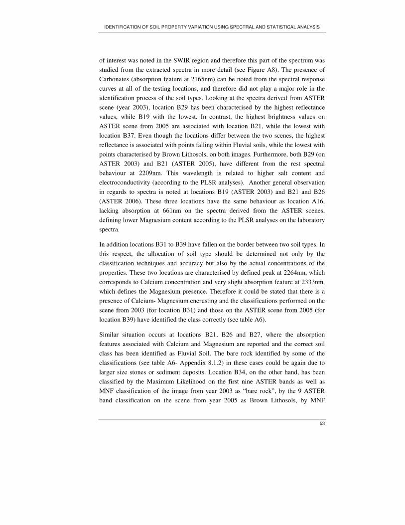
IDENTIFICATION OF SOIL PROPERTY VARIATION USING SPECTRAL AND STATISTICAL ANALYSIS
53
of interest was noted in the SWIR region and therefore this part of the spectrum was
studied from the extracted spectra in more detail (see Figure A8). The presence of
Carbonates (absorption feature at 2165nm) can be noted from the spectral response
curves at all of the testing locations, and therefore did not play a major role in the
identification process of the soil types. Looking at the spectra derived from ASTER
scene (year 2003), location B29 has been characterised by the highest reflectance
values, while B19 with the lowest. In contrast, the highest brightness values on
ASTER scene from 2005 are associated with location B21, while the lowest with
location B37. Even though the locations differ between the two scenes, the highest
reflectance is associated with points falling within Fluvial soils, while the lowest with
points characterised by Brown Lithosols, on both images. Furthermore, both B29 (on
ASTER 2003) and B21 (ASTER 2005), have different from the rest spectral
behaviour at 2209nm. This wavelength is related to higher salt content and
electroconductivity (according to the PLSR analyses). Another general observation
in regards to spectra is noted at locations B19 (ASTER 2003) and B21 and B26
(ASTER 2006). These three locations have the same behaviour as location A16,
lacking absorption at 661nm on the spectra derived from the ASTER scenes,
defining lower Magnesium content according to the PLSR analyses on the laboratory
spectra.
In addition locations B31 to B39 have fallen on the border between two soil types. In
this respect, the allocation of soil type should be determined not only by the
classification techniques and accuracy but also by the actual concentrations of the
properties. These two locations are characterised by defined peak at 2264nm, which
corresponds to Calcium concentration and very slight absorption feature at 2333nm,
which defines the Magnesium presence. Therefore it could be stated that there is a
presence of Calcium- Magnesium encrusting and the classifications performed on the
scene from 2003 (for location B31) and those on the ASTER scene from 2005 (for
location B39) have identified the class correctly (see table A6).
Similar situation occurs at locations B21, B26 and B27, where the absorption
features associated with Calcium and Magnesium are reported and the correct soil
class has been identified as Fluvial Soil. The bare rock identified by some of the
classifications (see table A6- Appendix 8.1.2) in these cases could be again due to
larger size stones or sediment deposits. Location B34, on the other hand, has been
classified by the Maximum Likelihood on the first nine ASTER bands as well as
MNF classification of the image from year 2003 as “bare rock”, by the 9 ASTER
band classification on the scene from year 2005 as Brown Lithosols, by MNF
IDENTIFICATION OF SOIL PROPERTY VARIATION USING SPECTRAL AND STATISTICAL ANALYSIS
54
classification of the image from 2005 as Fluvial soil while the map indicates border
between Fluvial and Brown Lithosolic soil. Referring to the spectral response,
however, it is noted that the signature matches perfectly the one at B39 on the image
from 2003, and differs greatly on the image from 2005. The reasons behind this can
be many. The most obvious one is the specific location of both sampling locations on
the border between Fluvial soil and Brown Lithosols. Furthermore, the difference in
the spectra is noted greatly at 807nm, associated with electroconductivity and
magnesium concentration, which consequently may indicate change in soil
composition over the two year period.
According to the reference soil map, sample B35 has been classified by all
classification techniques as “Bare Rock” instead of fluvial soil (as indicated on the
soil amp). The spectral curve indicates deep absorption at 2264nm related to high
Calcium concentration and considering the relatively high Carbonate concentration
defined earlier for all locations from the spectra, it could be assumed that the pixel
containing the location could be comprised of bare rock (probably limestone) or
thick Calcium crusting. To improve the prediction at this, as well as all the other
locations, more detailed geological investigation should be carried out.

IDENTIFICATION OF SOIL PROPERTY VARIATION USING SPECTRAL AND STATISTICAL ANALYSIS
55
5. Conclusions
Overall, ten soil properties were identified as important in relation to the main soil
types typical for the location of the study area- in South-East Tunisia. These include
electroconductivity (EC), Sodium (Na), Calcium (Ca), Carbonates, and Magnesium
(Mg), distinctive for the dominant soil group- Aridisols. In terms of the Entisols, Iron
(Fe), Potassium (K) and organic matter (OM) were studied. In addition, the moisture
content and pH of the soil were selected due to their strong influence on the soil
reflectance in general. Applying the standard techniques for analysis in the
laboratory, the concentrations of most of these properties were estimated as trace,
and for Fe these were even lower than the detection limit of the analytical apparatus,
for nine (plus one duplicate) samples.
Although a limited amount of material was available for laboratory analysis, the
concentration estimation, together with spectral information obtained under
laboratory conditions, was enough for the development of Partial Least Squared
Regression (PLSR) prediction models. The albedo was estimated (by CIE
chromaticity diagram) and since small variation was observed, it has been removed
from the PLS analysis. The ratio of prediction to deviation (RPD), in combination
with the coefficient of determination (R2), was used for the assessment of the
prediction model. These have indicated satisfying results for MC, OM, K and Na. A
number of significant wavelengths for the prediction model were also identified by
plotting the regression coefficients produced by the PLSR and examining the highest
peaks and the deepest sinks on the plot, most of them related to the shortwave
infrared region (2000-2500nm).
Two ASTER scenes (year 2003 and 2005) were pre-processed applying Log
Residual Atmospheric correction, Histogram matching and Minimum Noise
Fraction. ISODATA unsupervised classification was performed in terms of
identifying homogeneous areas and selecting appropriate regions of interest in
combination with soil maps from year 1975 (1:500,000). Maximum Likelihood
algorithm was chosen for the supervised classification. Generally, the classification
techniques applied on the ASTER scene from year 2003 showed better overall
accuracies than those applied on the scene from 2005, applying three different
accuracy assessment techniques: according to regions of interest, according to the
reference soil map and exploring the Rule images created in addition to the

IDENTIFICATION OF SOIL PROPERTY VARIATION USING SPECTRAL AND STATISTICAL ANALYSIS
56
classifications. It has been established that the selection and separability of the
regions of interest are crucial for achieving accurate results.
To overcome the gap between the laboratory measurements and the information
derived from the ASTER scenes, the spectral library obtained under laboratory
conditions was resampled to ASTER, so that the spectral resolution is reduced. This
was input into the PLSR model. The libraries derived from the scenes were also
tested against the measured properties. The result indicated stronger relationships
between the properties and the spectra as well as reduction in the number of
important wavelengths associated with the properties of interest.
PLSR coefficients were plotted against each other resulting in good predictions and
strong relationships established between spectra and electroconductivity, Calcium
and Magnesium (R2>0.9 and RPD>3.18). The important wavelengths for most of the
properties have been recognised in the shortwave infrared region of the spectrum,
and the absorption features corresponding to these wavelengths have been studied, in
terms of explaining the bands that overlap for different properties.
The link between the classification techniques and the PLSR analyses has been
established by determining the soil types, and the related soil properties assigned to
the sampling locations. The emerging problems are mainly related to the old soil map
used as reference; the scale of 1:500,000 compared to the 30m spatial resolution of
ASTER (in the SWIR region); the similarity between the soil types and general lack
of validation and analytical data. These prevented the study from drawing significant
conclusions. With 95% confidence, only small amount of pixels that belong to the
main soil types present in the study area can be considered as correctly classified,
resulting in one out of ten samples ‘probably’ assigned accurately. With 85%
confidence, the number of samples classified correctly is three. The applicability
and performance of the method have been tested with additional 25 sampling points.
The use of ASTER imagery in soil properties variation detection has indeed a great
potential related to the many applications such study can have in agriculture
management, soil erosion monitoring, soil salinisation, soil pollution detection, etc..
Many drawbacks, mainly associated with the quality of the available data, limit the
scope of this study, however the findings suggest that more detailed study
implementing this analytical methodology could greatly widen the prospective of
using readily available multispectral remotely sensed data.

IDENTIFICATION OF SOIL PROPERTY VARIATION USING SPECTRAL AND STATISTICAL ANALYSIS
57
6. Recommendations
• Further study should have a larger dataset available for analysis and
validation
• More recent soil maps as well as geological maps should be made available
• A larger and more heterogeneous study area or a combination of a number
of homogeneous but different in terms of soil types and properties soil
clusters should be selected, so that the class separability computation could
launch useful results.
• The image classifications should be performed according to soil properties
rather than soil types.
• Future study can also emphasise on the potential of PLSR coefficients in
terms of gaining information about actual concentrations of certain
elements
• More accurate results could be obtained if terrain parameters such as digital
elevation model, slope and aspect are included in the analysis of the
ASTER scenes.
• The potential of different band combinations associated with the properties
of interest could be studied in terms of improving the accuracy of the
prediction.
• The possibilities of better accuracy assessment related to Rule images
analyses are many. Further study could emphasise on analyses related to
overlapping of correctly classified pixels derived from a number of different
classifications.
• Field spectrometer measurements, areal photographs and hyperspectral
imagery could be applied in terms of minimising the gap between the fine
spectral resolution of the laboratory measurements and the coarse resolution
of the ASTER images.

IDENTIFICATION OF SOIL PROPERTY VARIATION USING SPECTRAL AND STATISTICAL ANALYSIS
59
7. References
• ACSAD Service of Mapping, 1986, Soil Map of Tunisia- 1:500,000, Soil
Science Division, Tunis
• Apan, A., Kelly, R., Jensen, T., Butler, D., Strong, W. & Basnet, B., 2002,
Spectral Discrimination and Seperability Analysis of Agricultural Crops and
Soil Attributes Using ASTER Imagery, 11th
Australian Remote Sensing and
Photogrammetry Association Conference, ISBN 0-9581366-0-2.397.
• Barnes, E., Sudduth, K., Hummel, J., Lesch, S., Corwin, D., Yang, C.,
Daughtry, C. & Bausch, W., 2003, Remote- and Ground-based Sensor
Technologies to Map Soil Properties, Photogrammetric Engineering and
Remote Sensing, 69(6): 619-630
• Baumgardner, M., Silva, L., Biehl, L. & Stoner, E., 1985, Reflectance
Properties of Soil, Advances in Agronomy, 38:1-44
• Ben-Dor, E. & Banin, A., 1995, Near Infrared analysis as a rapid method to
simultaneously evaluate several soil properties, American Journal of Soil
Science Society,159: 259-269
• Ben-Dor, E., Patkin, K., Banin, A. & Karnieli, A., 2002, Mapping of Several
Soil Properties Using DAIS-7915 Hyperspectral Scanner Data- A Case Study
Over Clayey Soils in Israel, International Journal of Remote Sensing, 26(6):
1043-1062
• Ben-Dor, E., Goldlshleger, N., Benyamini, Y., Agassi, M. & Blumberg, D.,
2003, The Spectral Reflectance Properties of Soil Structural Crust in the 1.2-2.5
µm Spectral Region, Soil Science Society American Journal, 67:289-294
• Brown, A. & Feringa, W., 2003, Colour Basics for GIS Users, Pearson
Education Limited, England
• California Institute of Technology, 2006, Advanced Spaceborne Thermal
Emission and Reflection Radiometer: Instrument Subsystems,
http://asterweb.jpl.nasa.gov/instrument.asp, [accessed 04/12/2006]

IDENTIFICATION OF SOIL PROPERTY VARIATION USING SPECTRAL AND STATISTICAL ANALYSIS
60
• Chabrillat, S., Goetz, A., Krosley, L. & Olsen, H., 2002, Use of hyperspectral
images in the identification and mapping of expansive clay soils and the role of
spatial resolution, Remote sensing of Environment, 82: 431-445
• Chang, D. & Islam, S., 2000, Estimation of Soil Physical Properties Using
Remote Sensing and Artificial Neural Network, Remote Sensing of
Environment, 74: 534-544
• Davies, A., 2001, Uncertainty testing in PLS regression, Spectroscopy Europe,
Norwich Near Infrared Consultancy
• De Jong, S. & Epema, G., 2001, Imaging Spectrometry for Surveying and
Modelling land degradation, In: Van der Meer, F. & de Jong, S., 2001,
Imaging Spectroscopy: Basic Principles and Prospective Applications, Kluwer
Academic Publishers, the Netherlands
• Department of Natural Resources, NSW Government 2007, Soil Survey:
Explanation of Exchangeable Cation Analysis and Interpretation,
http://naturalresources.nsw.gov.au/soils/index.shtml, [accessed 24/01/2007]
• ENVI 4.1 Tutorial- HELP, 2007
• Farifteh, J., Van der Meer, F., Atzberg, C. & Carranza, E., 2006, Quantitative
analysis of salt-affected soil reflectance spectra: A comparison of two adaptive
methods- PLSR & ANN, Remote Sensing of Environment, [on review].
• Gomez, C., Delacourt, C., Allemand, P., Ledru, P. & Wackerle, R., 2005, Using
ASTER Remote Sensing Data Set for Geological Mapping in Namibia, Physics
and Chemistry of the Earth, 30: 97- 108
• Klein, C., 2006, Unsupervised Classification: Iterative Self-Organising Data
Analysis Technique,
http://geog.tamu.edu/klein/geog661/lecture_notes/lecture22/lecture22.pdf,
[accessed 10/01/2007]
• Lee, W., Sanchez, J.F., Mylavarapu, R.S. & Choe, J., 2003, Estimating
Chemical Properties of Florida Soils Using Spectral Response, American
Society of Agricultural Engineers, 46(5); 1443-1453
• Lopez-Granados, F., Jurado-Exposito, M., Pena-Barragan, J. & Garcia-Torres,
L., 2005, Using Geostatistical and Remote Sensing Approaches for Mapping
Soil Properties, European Journal of Agronomy, 23: 279-289
• Mainam, F., 1999, Modelling Soil Erodibility in the Semiarid Zone of
Cameroon, PHD Thesis, Ghent University, 90-6164-179-9

IDENTIFICATION OF SOIL PROPERTY VARIATION USING SPECTRAL AND STATISTICAL ANALYSIS
61
• Ministry of Agriculture, 1973, Soil Map of Tunisia- 1:1,000,000, Soil Science
Division, Tunis
• Palacios- Orueta, A. & Ustin, S., 1998, Remote Sensing of Soil Properties in
the Santa Monica Mountains I, Remote Sensing the Environment, 65: 170-183
• Palacios- Orueta, A., Pinzon, J., Ustin, S. & Roberts, D., 1999, Remote Sensing
of Soils in the Santa Monica Mountains: II. Hierarchical Foreground and
Background Analysis, Remote Sensing the Environment, 68: 138-151
• Post, D., Fimbres, A., Matthias, A., Sano, E., Accioly, L., Batchily, A. &
Ferreira, L., 2000, Predicting Soil Albedo from Soil Colour and Spectral
Reflectance Data, Soil Science Society American Journal, 4: 1027-1034
• Ramsey, 2006, Advanced Image Processing Techniques, Applied Remote
Sensing and GPS Techniques, GEO2460,
http://ivis.eps.pitt.edu/courses/ars/lectures/8.pdf, [accessed 10/01/2007]
• Savitzky, A. & Golay, M., 1964, Smoothing and Differentiation of Data by
Simplified Least Squares Procedures, Analytical Chemistry, 36: 1627-1639
• Scholte, K., 2005, Hyperspectral Remote Sensing and Mud Volcanism in
Azerbaijan, PhD Thesis, ITC, The Netherlands
• Shepherd, K. & Walsh, M., 2002, Division S-8-Nutrient Management and Soil
and Plant analysis: Development of Reflectance Spectral Libraries for
Characterisation of Soil Properties, Soil Science Society American Journal, 66:
988-998
• Soil Survey Staff, 1999, Soil Taxonomy: A Basic System of Soil Classification
for Making and Interpreting Soil Surveys, United States Department of
Agriculture, Washington DC, 20402
• Udelhoven, T., Emmerling, C. & Jarmer, T., 2003, Quantitative analysis of soil
chemical properties with diffuse reflectance spectrometry and partial least-
square regression: A feasibility study, Plant and soil, 251: 319-329
• USGS, 2006, Sensors- ASTER, http://eo1.usgs.gov/ASTER.php , [accessed
12/7/06]
• Van der Meer, F., de Jong & Bakker, W., 2001, Imaging Spectrometry: Basic
Analytical Techniques, In: Van der Meer, F. & de Jong, S., 2001, Imaging
Spectroscopy: Basic Principles and Prospective Applications, Kluwer
Academic Publishers, the Netherlands

IDENTIFICATION OF SOIL PROPERTY VARIATION USING SPECTRAL AND STATISTICAL ANALYSIS
62
• Van der Werff, H. 2006, Knowledge-based remote sensing of complex objects:
Recognition of spectral and spatial patterns resulting from natural
hydrocarbon seepages, PHD Thesis, ITC, Netherlands
• Van Reeuwijk, L.P., 2002, Procedures for soil analysis, International Soil
Reference and Information Centre- ISRIC, Technical paper 9, Sixth Edition,
USA
• Viscarra Rossel, R.A. 2005. ParLeS version 2.1a. Software for Chemometric
Analysis of Spectroscopic Data.
http://www.usyd.edu.au/su/agric/acpa/people/rvrossel/soft01.htm, [accessed
11/2006]
• Viscarra Rossel, R.A., Walvoort, D.J, McBratney, A.B, Janik, L.J. &
Skiemstad, J.O. 2006, Visible, Near infrared or combined diffuse reflectance
spectroscopy for simultaneous assessment of various soil properties, Geoderma
131:59-75
• Williams, P. 2001, Implementation of Near Infrared technology, In: Williams,
P. & Norris, K., 2001, Near Infrared technology in the agricultural and food
industries, American Association of Cereal Chemists, Minnesota
• Wold, S., Sjostrom, M. & Eriksson, L., 2001, PLS-regression: a basic tool of
chemometrics, Chemometrics and Intelligent Laboratory Systems, 58: 109-130
• Zhou, L., Dickenson, R. & Tian, J., 2005, Derivation of a soil albedo dataset
from MODIS using principle component analysis: Northern Africa and The
Arabian Peninsula, Geophysical research letters, 32, L21407

IDENTIFICATION OF SOIL PROPERTY VARIATION USING SPECTRAL AND STATISTICAL ANALYSIS
63
8. Appendices
8.1. Appendix 1: Selected figures and tables
8.1.1. Figures
Figure A1:a) Soil map 1:500000- ASTER coverage; b) Soil map 1:1000000- ASTER
coverage; c) Soil map 1:500000- Study area; d) Soil map 1:1000000- Study area
Sources of maps: Ministry of Agriculture, 1973; ACSAD, 1986

IDENTIFICATION OF SOIL PROPERTY VARIATION USING SPECTRAL AND STATISTICAL ANALYSIS
64
Figure A2: Flowchart of PLSR data arrangement procedure (Wold et al., 2001).
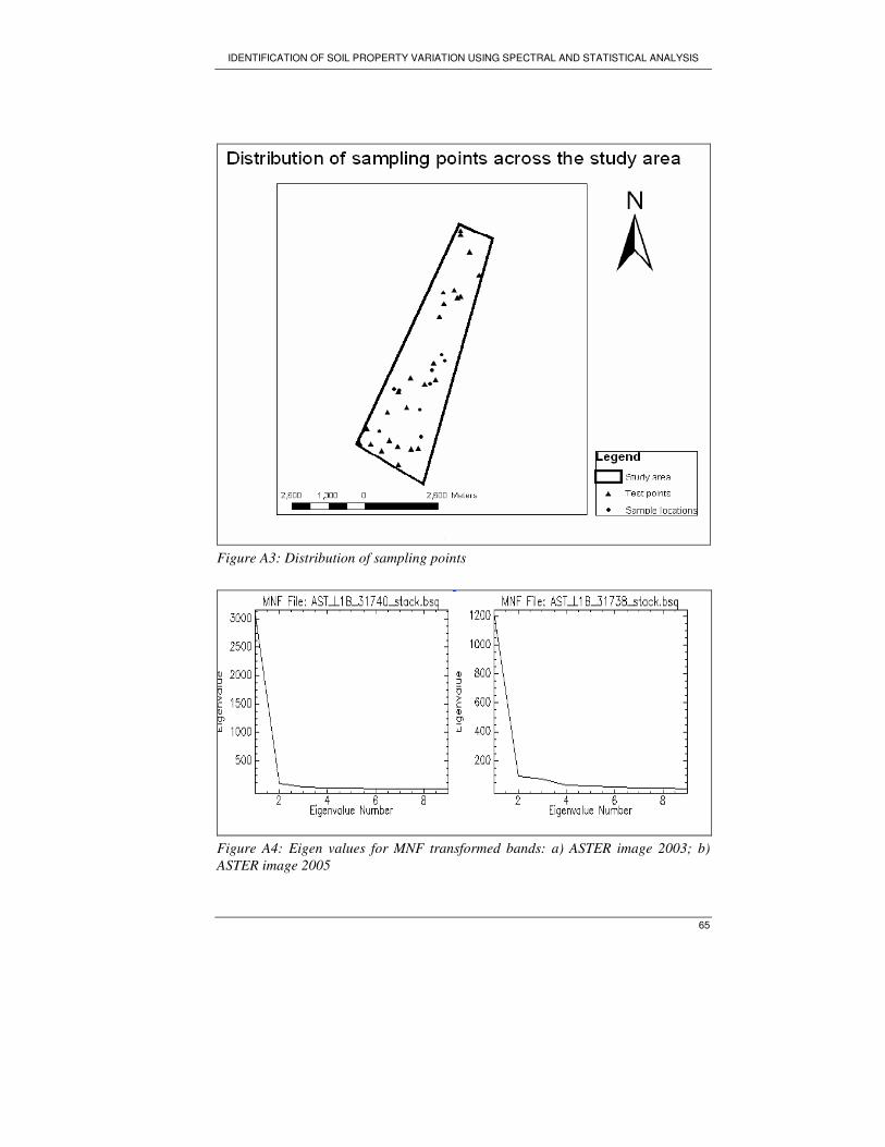
IDENTIFICATION OF SOIL PROPERTY VARIATION USING SPECTRAL AND STATISTICAL ANALYSIS
65
Figure A3: Distribution of sampling points
Figure A4: Eigen values for MNF transformed bands: a) ASTER image 2003; b)
ASTER image 2005

IDENTIFICATION OF SOIL PROPERTY VARIATION USING SPECTRAL AND STATISTICAL ANALYSIS
66
Figure A6: CIE diagram and soil samples colour distribution showing no difference
in soil colour
Figure A5: a) CIE tristimulus
curves (Van der Werff, 2006);
b) CIE chromaticity diagram
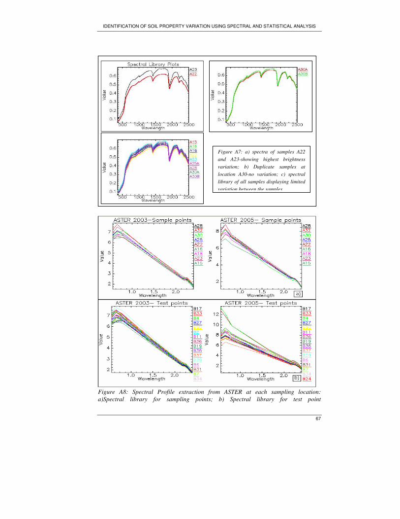
IDENTIFICATION OF SOIL PROPERTY VARIATION USING SPECTRAL AND STATISTICAL ANALYSIS
67
Figure A8: Spectral Profile extraction from ASTER at each sampling location:
a)Spectral library for sampling points; b) Spectral library for test point
Figure A7: a) spectra of samples A22
and A23-showing highest brightness
variation; b) Duplicate samples at
location A30-no variation; c) spectral
library of all samples displaying limited
variation between the samples


IDENTIFICATION OF SOIL PROPERTY VARIATION USING SPECTRAL AND STATISTICAL ANALYSIS
69
Figure A9: Analysis of the three spectral libraries (continuum removed) for selected
sampling points.
Figure A10: Misclassified pixels associated with Lithosols [green], Brown Lithosols
[blue] and Lithosols/Regosols [red]; a) ASTER 2003; b) ASTER 2005

IDENTIFICATION OF SOIL PROPERTY VARIATION USING SPECTRAL AND STATISTICAL ANALYSIS
70
8.1.2. Tables
Table A1: PLSR prediction model for Electroconductivity (EC), Moisture Content
(MC), Organic Matter (OM), Carbonate, Calcium (Ca), Potassium (K), Magnesium
(Mg), Manganese (Mn), Sodium (Na), using ASD FIELDSPEC spectrometer
measurements under laboratory conditions. SD (standard deviation) RMSE (root
mean square error), RPD (relative performance determinant).
Table A2: PLSR prediction model for Electroconductivity (EC), Moisture Content
(MC), Organic Matter (OM), Carbonate, Calcium (Ca), Potassium (K), Magnesium
(Mg), Manganese (Mn), Sodium (Na), using ASD FIELDSPEC spectrometer
measurements under laboratory conditions. Resampled to ASTER library. SD
(standard deviation) RMSE (root mean square error), RPD (relative performance
determinant)
Element Factors Variance SD R² RMSE RPD*
EC 5 193.35 13.91 0.80 6.64 2.38
MC 5 0.1 0.32 0.95 0.06 5.05
OM 5 0.4 0.63 0.83 0.27 2.60
Carbonate 5 1.6 1.27 0.71 0.79 1.97
Ca 5 13.74 3.71 0.74 2.05 2.09
K 5 1.62 1.27 0.82 0.55 2.49
Mg 5 0.59 0.77 0.62 0.57 1.71
Mn 5 0.01 0.11 0.71 0.07 1.96
Na 5 0.86 0.93 0.93 0.25 3.86
Element Factors Variance SD R2
RMSE RPD*
EC 5 226.11 15.04 0.92 4.17 3.79
MC 5 0.07 0.27 0.63 0.19 1.74
OM 5 0.35 0.59 0.73 0.34 2.04
Carbonate 5 0.87 0.93 0.41 1.13 1.37
Ca 5 14.26 3.78 0.77 1.94 2.22
K 5 1.17 1.08 0.49 0.93 1.48
Mg 5 0.23 0.48 0.16 0.84 1.51
Mn 5 0.01 0.1 0.56 0.08 1.6
Na 5 0.76 0.87 0.75 0.46 2.12

IDENTIFICATION OF SOIL PROPERTY VARIATION USING SPECTRAL AND STATISTICAL ANALYSIS
71
Table A3: PLSR prediction model for Electroconductivity (EC), Moisture Content
(MC), Organic Matter (OM), Carbonate, Calcium (Ca), Potassium (K), Magnesium
(Mg), Manganese (Mn), Sodium (Na): Spectral library derived from ASTER image
2003. SD (standard deviation) RMSE (root mean square error), RPD (relative
performance determinant)
*RPD classification for indicating the model prediction abilities (<1.5v bad; 1.5-2 bad; 2-2.5 good;
>2.5v good)
Table A4: PLSR prediction model for Electroconductivity (EC), Moisture Content
(MC), Organic Matter (OM), Carbonate, Calcium (Ca), Potassium (K), Magnesium
(Mg), Manganese (Mn), Sodium (Na): Spectral library derived from ASTER image
2005. SD (standard deviation) RMSE (root mean square error), RPD (relative
performance determinant)
Element Factors Variance SD R2
RMSE RPD*
EC 5 238.75 15.15 0.88 5.22 3.03
MC 5 0.08 0.29 0.73 0.16 2.05
OM 5 0.38 0.61 0.80 0.29 2.35
Carbonate 5 1.63 1.28 0.66 0.85 1.82
Ca 5 13.79 3.71 0.68 2.30 1.87
K 5 1.00 1.00 0.59 0.84 1.65
Mg 5 0.37 0.61 0.43 0.69 1.40
Mn 5 0.01 0.11 0.69 0.07 1.90
Na 5 0.75 0.87 0.74 0.47 2.07
Element Factors Variance SD R2
RMSE RPD*
EC 5 203.82 14.28 0.89 4.97 3.18
MC 5 0.05 0.22 0.43 0.24 1.40
OM 5 0.24 0.49 0.46 0.48 1.44
Carbonate 5 1.95 1.40 0.86 0.55 2.81
Ca 5 16.64 4.08 0.94 1.00 4.29
K 5 0.99 0.99 0.66 0.77 1.79
Mg 5 0.94 0.07 0.99 0.06 15.37
Mn 5 0.01 0.11 0.80 0.06 2.35
Na 5 0.68 0.82 0.73 0.48 2.02


IDENTIFICATION OF SOIL PROPERTY VARIATION USING SPECTRAL AND STATISTICAL ANALYSIS
73
Table A5: Extraction of soil types for each classification per sample point
Point MAXLIK
2003
MAXLIK 2005 MNF ASTER 2003 MNF ASTER 2005 Map scale 1:500000
A15 Fluvial soil Fluvial soil Fluvial soil Brown Lithosols Brown Lithosols
A16 Fluvial soil Fluvial soil Fluvial soil Fluvial soil Brown Lithosols
border with Fluvial
A18 Fluvial soil Fluvial soil Fluvial soil Fluvial soil Brown Lithosols
A22 Gypsiorthids Brown
Lithosols
Lithosols Brown Lithosols Fluvial soil/border
with Brown Lithosols
A23 Bare Rock Brown
Lithosols
Bare Rock Brown Lithosols Fluvial soil/Calci-
Magnesium
encrusting
A25 Bare Rock Fluvial soil Bare Rock Fluvial soil Fluvial soil/Calci-
Magnesium
encrusting
A28 Fluvial soil Fluvial soil Fluvial soil Brown Lithosols Fluvial soil/Calci-
Magnesium
encrusting
A30 Bare Rock Brown
Lithosols
Brown Lithosols Brown Lithosols Fluvial soil/Calci-
Magnesium
encrusting
A32 Gypsiorthids Bare Rock Brown Lithosols Brown Lithosols Fluvial soil/Calci-
Magnesium
encrusting

IDENTIFICATION OF SOIL PROPERTY VARIATION USING SPECTRAL AND STATISTICAL ANALYSIS
74
Table A6: Extraction of soil types for each classification per test sample point
Point
MAXLIK
2003
MAXLIK
2005 MNF 2003 MNF 2005 Soil Map
B1 Recent soil Cloud Recent soil Cloud Fluvial soil/Ca-Mg
B2 Fluvial Soil Cloud Fluvial Soil Cloud Fluvial soil/Ca-Mg
B3 Recent soil Cloud Recent soil Cloud Fluvial soil/Ca-Mg
B4 Fluvial Soil Fluvial Soil Fluvial Soil Fluvial Soil Fluvial soil/Ca-Mg
B5 Fluvial Soil Cloud Fluvial Soil Cloud Fluvial soil/Ca-Mg
B6 Fluvial Soil Cloud Fluvial Soil Cloud Fluvial soil/Ca-Mg
B7 Fluvial Soil Fluvial Soil Fluvial Soil Fluvial Soil Fluvial soil/Ca-Mg
B8 Fluvial Soil Fluvial Soil Fluvial Soil Fluvial Soil Fluvial soil/Ca-Mg
B9 Fluvial Soil Fluvial Soil Bare Rock Fluvial Soil Fluvial soil/Ca-Mg
B11 Fluvial Soil
Brown
Lithosols Recent soil Brown Lithosols Fluvial soil/Ca-Mg
B17 Bare Rock Bare Rock Bare Rock Bare Rock Brown Lithosols
B19 Fluvial Soil
Brown
Lithosols Fluvial Soil Brown Lithosols Brown Lithosols
B20 Fluvial Soil Fluvial Soil Fluvial Soil Fluvial Soil Fluvial soil/Ca-Mg
B21 Recent soil Bare Rock Recent soil Bare Rock Fluvial soil/Ca-Mg
B24 Fluvial Soil Fluvial Soil Fluvial Soil Fluvial Soil Fluvial soil/Ca-Mg
B26 Bare Rock Fluvial Soil Gypsiorthids Fluvial Soil Fluvial soil/Ca-Mg
B27 Bare Rock Fluvial Soil Bare Rock Fluvial Soil Fluvial soil/Ca-Mg

IDENTIFICATION OF SOIL PROPERTY VARIATION USING SPECTRAL AND STATISTICAL ANALYSIS
75
B29 Fluvial Soil Bare Rock Recent soil Bare Rock Fluvial soil/Ca
B31 Fluvial Soil
Brown
Lithosols Fluvial Soil Brown Lithosols
Fluvial soil/Ca
B33 Bare Rock
Brown
Lithosols Bare Rock Brown Lithosols
Fluvial border
with Brown Lithosols
B34 Bare Rock
Brown
Lithosols Bare Rock Fluvial Soil
Fluvial border
with Brown Lithosols
B35 Bare Rock Bare Rock Bare Rock Bare Rock
Fluvial border
with Brown Lithosols
B36 Fluvial Soil
Brown
Lithosols Fluvial Soil Brown Lithosols
Fluvial border
with Brown Lithosols
B37 Bare Rock Fluvial Soil Recent soil Bare Rock
Fluvial border
with Brown Lithosols
B38 Fluvial Soil Fluvial Soil Fluvial Soil Fluvial Soil
Fluvial border
with Brown Lithosols
B39 Bare Rock Fluvial Soil Bare Rock Fluvial Soil
Fluvial border
with Brown Lithosols

IDENTIFICATION OF SOIL PROPERTY VARIATION USING SPECTRAL AND STATISTICAL ANALYSIS
76
8.2. Appendix 2: Field work report
Sample
ID Date X Y Grain size pH
Soil
colour
Visible
contamination/Other
comments
Projectio
n
GPS
accuracy
A15 28/09/2006 600891 3724263
Fine:
<2mm, dry
lumps
NOT IN
FIELD
VERY
PALE
BROWN
Land prepared for
agriculture, some dry
small grass, dry lumps WGS 84 6m
A16 28/09/2006 600550 3723646
Fine:
<2mm, dry
lumps
NOT IN
FIELD
VERY
PALE
BROWN
Land prepared for
agriculture, some
stones WGS 84 7m
A18 28/09/2006 601003 3723984
Fine:
<2mm, dry
lumps
NOT IN
FIELD
VERY
PALE
BROWN
Land prepared for
agriculture, some
stones, dry grass WGS 84 6m
A22 28/09/2006 600483 3723119
Fine:
<2mm, dry
lumps
NOT IN
FIELD
VERY
PALE
BROWN
Land prepared for
agriculture, some
stones, small bushes,
stones WGS 84 6m
A23 28/09/2006 599203 3722903
Fine:
<2mm, dry
lumps
NOT IN
FIELD
VERY
PALE
BROWN
Land prepared for
agriculture (olive
trees), lumps of dry
soil WGS 84 8m
A25 28/09/2006 599386 3722868
Fine:
<2mm, dry
lumps
NOT IN
FIELD
VERY
PALE
BROWN
Dry small bushes,
lumps of dry soil and
stones WGS 84 7m

IDENTIFICATION OF SOIL PROPERTY VARIATION USING SPECTRAL AND STATISTICAL ANALYSIS
77
A28 28/09/2006 600121 3722139
Fine:
<2mm, dry
lumps
NOT IN
FIELD
VERY
PALE
BROWN
Land prepared for
agriculture, lumps of
dry soil, trees close by WGS 84 6m
A30 27/09/2006 598675 3721309
Fine:
<2mm, dry
lumps
NOT IN
FIELD
VERY
PALE
BROWN
Land prepared for
agriculture, some
palm trees near by,
crust WGS 84 7m
A32 27/09/2006 600159 3721074
Fine:
<2mm, dry
lumps
NOT IN
FIELD
VERY
PALE
BROWN
Some dry vegetation,
stones and crust WGS 84 6m
B1 26/09/2006 601576 3728960
Fine:
<2mm
NOT IN
FIELD
VERY
PALE
BROWN
Small bushes, dry
crust, no stones WGS 84 6m
B2 26/09/2006 601558 3728815
Fine:
<2mm
NOT IN
FIELD
VERY
PALE
BROWN
Small bushes, dry
crust, stones are
present WGS 84 6m
B3 26/09/2006 601916 3728174
Fine:
<2mm, dry
lumps
NOT IN
FIELD
VERY
PALE
BROWN
Land prepared for
agriculture, some
stones and dry lumps
of soil WGS 84 6m

IDENTIFICATION OF SOIL PROPERTY VARIATION USING SPECTRAL AND STATISTICAL ANALYSIS
78
B4 26/09/2006 602259 3727279
Fine:
<2mm,
stones
NOT IN
FIELD
VERY
PALE
BROWN
Big stones, dry
bushes, crust WGS 84 10m
B5 26/09/2006 601346 3726698
Fine:
<2mm, dry
lumps
NOT IN
FIELD
VERY
PALE
BROWN
Some dry lichen, crust
and big lumps of dry
soil WGS 84 6m
B6 26/09/2006 600969 3726616
Fine:
<2mm
NOT IN
FIELD
VERY
PALE
BROWN
Some dry vegetation,
stones and crust WGS 84 6m
B7 26/09/2006 601473 3726399
Fine:
<2mm, dry
lumps
NOT IN
FIELD
VERY
PALE
BROWN
Crust and a lot of dry
vegetation and roots WGS 84 10m
B8 26/09/2006 601574 3726443
Fine:
<2mm, dry
lumps
NOT IN
FIELD
VERY
PALE
BROWN
Crust and dry
vegetation WGS 84 10m
B9 26/09/2006 600998 3726168
Fine:
<2mm, dry
lumps
NOT IN
FIELD
VERY
PALE
BROWN
Land prepared for
agriculture, some
crust, small trees and
some stones WGS 84 6m
B11 26/09/2006 600807 3725665
Fine:
<2mm, dry
lumps
NOT IN
FIELD
VERY
PALE
BROWN Crust, no vegetation WGS 84 6m

IDENTIFICATION OF SOIL PROPERTY VARIATION USING SPECTRAL AND STATISTICAL ANALYSIS
79
B17 28/09/2006 600622 3723922
Fine:
<2mm, dry
lumps
NOT IN
FIELD
VERY
PALE
BROWN
Land prepared for
agriculture, some
stones, some small
bushes WGS 84 6m
B19 28/09/2006 600684 3723274
Fine:
<2mm, dry
lumps
NOT IN
FIELD
VERY
PALE
BROWN
Land prepared for
agriculture, some
grass and small
bushes WGS 84 7m
B20 28/09/2006 600316 3723169
Fine:
<2mm, dry
lumps
NOT IN
FIELD
VERY
PALE
BROWN
Some grass and small
bushes, and trees WGS 84 6m
B24 28/09/2006 599372 3722846
Fine:
<2mm, dry
lumps
NOT IN
FIELD
VERY
PALE
BROWN
Dry small bushes,
lumps of dry soil and
stones WGS 84 8m
B26 28/09/2006 599676 3722231
Fine:
<2mm, dry
lumps
NOT IN
FIELD
VERY
PALE
BROWN
Land prepared for
agriculture, dry grass
and trees near by WGS 84 8m
B27 28/09/2006 598970 3722035
Fine:
<2mm, dry
lumps
NOT IN
FIELD
VERY
PALE
BROWN
Land prepared for
agriculture, some
trees and buildings WGS 84 7m

IDENTIFICATION OF SOIL PROPERTY VARIATION USING SPECTRAL AND STATISTICAL ANALYSIS
80
B29 28/09/2006 598250 3721413
Fine:
<2mm, dry
lumps
NOT IN
FIELD
VERY
PALE
BROWN
Land prepared for
agriculture, some
small bushes, crust,
lumps WGS 84 6m
B31 27/09/2006 599045 3720967
Fine:
<2mm, dry
lumps
NOT IN
FIELD
VERY
PALE
BROWN
Lumps and crust,
some green and dry
vegetation, buildings
near by WGS 84 6m
B33 27/09/2006 598385 3720822
Fine:
<2mm, dry
lumps
NOT IN
FIELD
VERY
PALE
BROWN
Land prepared for
agriculture, lumps of
dry soil, stones WGS 84 7m
B34 27/09/2006 598775 3720577
Fine:
<2mm, dry
lumps
NOT IN
FIELD
VERY
PALE
BROWN
Some dry and green
vegetation, lumps of
dry soil, land prepared
for agriculture WGS 84 10m
B35 27/09/2006 599343 3720737
Fine:
<2mm, dry
lumps
NOT IN
FIELD
VERY
PALE
BROWN
Land prepared for
agriculture, crust and
lumps of dry soil,
some trees around WGS 84 7m
B36 27/09/2006 599814 3720654
Fine:
<2mm, dry
lumps
NOT IN
FIELD
VERY
PALE
BROWN
Some dry bushes and
stones, some trees and
buildings near by WGS 84 7m

IDENTIFICATION OF SOIL PROPERTY VARIATION USING SPECTRAL AND STATISTICAL ANALYSIS
81
B37 27/09/2006 600087 3720676
Fine:
<2mm, dry
lumps
NOT IN
FIELD
VERY
PALE
BROWN
Some dry bushes,
trees and buildings
near by, dry lichen WGS 84 6m
B38 27/09/2006 599374 3720059
Fine:
<2mm, dry
lumps
NOT IN
FIELD
VERY
PALE
BROWN
Some dry bushes,
trees and buildings
near by, dry lichen WGS 84 7m
B39 27/09/2006 598003 3720844
Fine:
<2mm, dry
lumps
NOT IN
FIELD
VERY
PALE
BROWN Dry vegetation WGS 84 6m


IDENTIFICATION OF SOIL PROPERTY VARIATION USING SPECTRAL AND STATISTICAL ANALYSIS
83
8.3. Appendix 3: Samples photographs

IDENTIFICATION OF SOIL PROPERTY VARIATION USING SPECTRAL AND STATISTICAL ANALYSIS
84
8.4. Appendix 4: Procedures for soil analysis
Reference: Van Reeuwijk, L.P. (2002)
pH
1. Weigh 20g fine soil into a 100ml polythene wide-mouth type bottle. Include
a blank
2. Add 50ml water and cap the bottle
3. Shake for 2 hours
4. Before opening the bottle for measurement, shake by hand once more
5. Immerse pH electrode in the upper part of suspension
6. Read pH when reading has stabilised
Electroconductivity
1. Add about 30ml standard 0.01M KCl solution to a 50ml beaker and
measure temperature
2. Rinse and fill pipette cell with the standard KCl solution or insert dip cell in
this solution
3. Set temperature compensation deal at measured temperature and adjust
reading of the meter
4. Measure the temperature of the extract and set temperature compensation
dial at this temperature
5. Fill pipette cell with extract or insert dip cell into extract and read
condictivity
Moisture Content
1. Transfer approximately 5g fine material to a tared moisture tin and weigh
2. Dry overnight at 105 degrees
3. Remove tin from the oven, close with a lid, cool in desiccators and weigh
4. Calculate moisture content (water loss)

IDENTIFICATION OF SOIL PROPERTY VARIATION USING SPECTRAL AND STATISTICAL ANALYSIS
85
Soil Organic Carbon/Organic Matter
1. 1g of soil material is places into a 500ml flask
2. Add 10ml dichloromate solution
3. Add 20ml sulphuric acid, swirl the flask and allow to stand on a pad for 30
minutes
4. Add 200 ml water and 10ml phosphoric acid
5. Add 1ml indicator solution and titrate with ferrous sulphate solution. Stir
until the brown colour turns purple or violet-blue. Slow down the titration
6. At the end point the colour changes to green
7. Use the formula to convert to Organic Matter:
%Organic Matter= 2x % Organic Carbon
Carbonate
1. Weigh 5g fine material into a shaking bottle
2. Add 100ml 0.2M HCL by pipette and swirl
3. Loosely screw on lid and swirl occasionally during the next hour. Let then
stand over night
4. The next day, indent the bottle by hand, tighten the lid and shake for 2 hours
in reciprocating shaker.
5. Let the suspension settle, pipette 10ml supernatant solution into 100ml
Erlenmeyer flask and add about 25ml water
6. Add a few drops phenolphthalein indicator and titrate with 0.1M NaOH
Calcium, Potassium, Magnesium, Manganese, Sodium by ICP-OES

IDENTIFICATION OF SOIL PROPERTY VARIATION USING SPECTRAL AND STATISTICAL ANALYSIS
86
1. For the digestion of solid samples, a representative 1 gram (wet weight)
sample is digested with repeated additions of nitric acid (HNO3) and
hydrogen peroxide (H2O2).
2. For ICP-OES analysis, hydrochloric acid (HCl) is added to the initial
digested solution and the sample is refluxed and then diluted to a final
volume of 200 mL. The digested sample is analyzed using the ICP-OES

IDENTIFICATION OF SOIL PROPERTY VARIATION USING SPECTRAL AND STATISTICAL ANALYSIS
87
8.5. Appendix 5: Classification Accuracies
MAXLIK 2003
Overall accuracy: 88.0482%; Kappa coefficient: 0.86
Ground Truth
(pixels)
Class Eroded rocky Lithosols Lithosols/Rig Brown Lithosols Gypsum/gley
Unclassified 0 0 0 0 0
Eroded rocky 62946 2 2713 754 25362
Lithosols [Gr 0 116602 44 5029 5
Lithosols/Rig 2090 127 105969 297 12702
Brown Lithosols 243 4004 1250 107432 1411
Gypsum/gley [ 17318 38 14225 2459 79141
Halomorphs/ u 0 0 0 0 0
Young soil 0 0 0 0 3
Fluvial soil 6160 0 23 4 805
Sols bruns je 778 1 15 41 81
Water/no data 0 0 0 0 0
Total 89535 120774 124239 116016 119510
Ground Truth
Class Halomorphs Young soil Fluvial soil Sols bruns je
Water/no
data
Unclassified 0 0 0 0 0
Eroded rocky 0 0 5041 370 0
Lithosols [Gr 0 0 0 0 0
Lithosols/Rig 0 0 71 0 68
Brown Lithosols 0 0 5 20 0
Gypsum/gley [ 0 0 548 28 6
Halomorphs/ u 8702 1 0 0 0
Young soil 0 4239 41 136 0
Fluvial soil 0 0 80668 394 0
Sols bruns je 0 10 2174 39546 0
Water/no data 0 0 0 0 182257
Total 8702 4250 88548 40494 182331

IDENTIFICATION OF SOIL PROPERTY VARIATION USING SPECTRAL AND STATISTICAL ANALYSIS
88
Ground Truth
Class Total
Unclassified 0
Eroded rocky 97188
Lithosols [Gr 121680
Lithosols/Rig 121324
Brown Lithosols 114365
Gypsum/gley [ 113763
Halomorphs/ u 8703
Young soil 4419
Fluvial soil 88054
Sols bruns je 42646
Water/no data 182257
Total 894399
Ground Truth%
Class Eroded rocky Lithosols Lithosols/Rig Brown Lithosols Gypsum/gley
Unclassified 0 0 0 0 0
Eroded rocky 70.3 0 2.18 0.65 21.22
Lithosols [Gr 0 96.55 0.04 4.33 0
Lithosols/Rig 2.33 0.11 85.29 0.26 10.63
Brown Lithosols 0.27 3.32 1.01 92.6 1.18
Gypsum/gley [ 19.34 0.03 11.45 2.12 66.22
Halomorphs/ u 0 0 0 0 0
Young soil 0 0 0 0 0
Fluvial soil 6.88 0 0.02 0 0.67
Sols bruns je 0.87 0 0.01 0.04 0.07
Water/no data 0 0 0 0 0
Total 100 100 100 100 100
Ground Truth%
Class Halomorphs/ uS ols peu evol Fluvial soil Sols bruns je
Water/no
data
Unclassified 0 0 0 0 0
Eroded rocky 0 0 5.69 0.91 0

IDENTIFICATION OF SOIL PROPERTY VARIATION USING SPECTRAL AND STATISTICAL ANALYSIS
89
Lithosols [Gr 0 0 0 0 0
Lithosols/Rig 0 0 0.08 0 0.04
Brown Lithosols 0 0 0.01 0.05 0
Gypsum/gley [ 0 0 0.62 0.07 0
Halomorphs/ u 100 0.02 0 0 0
Young soil 0 99.74 0.05 0.34 0
Fluvial soil 0 0 91.1 0.97 0
Sols bruns je 0 0.24 2.46 97.66 0
Water/no data 0 0 0 0 99.96
Total 100 100 100 100 100
Ground Thruth %
Class Total
Unclassified 0
Eroded rocky 10.87
Lithosols [Gr 13.6
Lithosols/Rig 13.56
Brown Lithosols 12.79
Gypsum/gley [ 12.72
Halomorphs/ u 0.97
Young soil 0.49
Fluvial soil 9.85
Sols bruns je 4.77
Water/no data 20.38
Total 100
Class Commission Omission Commission Omission
(Percent) (Percent) (Pixels) (Pixels)
Eroded rocky 35.23 29.7 34242/97188 26589/89535
Lithosols [Gr 4.17 3.45 5078/121680 4172/120774
Lithosols/Rig 12.66 14.71 15355/121324 18270/124239
Brown Lithosols 6.06 7.4 6933/114365 8584/116016
Gypsum/gley [ 30.43 33.78 34622/113763 40369/119510
Halomorphs/ u 0.01 0 01 8703 0/8702

IDENTIFICATION OF SOIL PROPERTY VARIATION USING SPECTRAL AND STATISTICAL ANALYSIS
90
Young soil 4.07 0.26 180/4419 11 4250
Fluvial soil 8.39 8.9 7386/88054 7880/88548
Sols bruns je 7.27 2.34 3100/42646 948/40494
Water/no data 0 0.04 0/182257 74/182331
Class Prod. Acc. User Acc. Prod. Acc. User Acc.
(Percent) (Percent) (Pixels) (Pixels)
Eroded rocky 70.3 64.77 62946/89535 62946/97188
Lithosols [Gr 96.55 95.83 116602/120774 116602/121680
Lithosols/Rig 85.29 87.34 105969/124239 105969/121324
Brown Lithosols 92.6 93.94 107432/116016 107432/114365
Gypsum/gley [ 66.22 69.57 79141/119510 79141/113763
Halomorphs/ u 100 99.99 8702/8702 8702/8703
Young soil 99.74 95.93 4239/4250 4239/4419
Fluvial soil 91.1 91.61 80668/88548 80668/88054
Sols bruns je 97.66 92.73 39546/40494 39546/42646
Water/no data 99.96 100 182257/182331 182257/182257
ASTER 2005
Ground Truth pixel
Class Eroded rocky Lithosols Lithosols/Rig Brown Lithosols Gypsum/gley
Unclassified 0 0 0 0 0
Eroded rocky 53568 1187 2493 8397 19963
Lithosols [Gr 998 106466 5622 16865 11637
Lithosols/Rig 1433 3478 111642 2976 32508
Brown Lithosols 11200 9225 2500 82225 30673
Gypsum/gley [ 2910 362 1847 2304 18851
Cloud [White] 1194 0 0 185 2280
Cloud shadow 255 0 0 0 58
Halomorphs/ u 0 0 0 0 0
Young soil 285 0 0 16 26
Sols bruns je 3354 0 8 170 622
Fluvial soil 14338 56 127 2878 2892

IDENTIFICATION OF SOIL PROPERTY VARIATION USING SPECTRAL AND STATISTICAL ANALYSIS
91
Total 89535 120774 124239 116016 119510
Ground Truth-
pixel
Class Cloud Cl
oud
shadow
Halomorphs/
u Young soil Sols bruns je
Unclassified 0 0 0 0 0
Eroded rocky 156 128 0 35 220
Lithosols [Gr 0 0 0 0 0
Lithosols/Rig 0 0 0 0 0
Brown Lithosols 9 0 0 1 13
Gypsum/gley [ 9 73 0 9 30
Cloud [White] 22575 41 24 118 673
Cloud shadow 0 23103 0 0 43
Halomorphs/ u 0 0 8678 0 0
Young soil 171 1 0 5479 2114
Sols bruns je 345 347 0 352 15208
Fluvial soil 12 1 0 3 184
Total 23277 23694 8702 5997 18485
Ground Truth-
pixel
Class Fluvial soil Total
Unclassified 0 0
Eroded rocky 6154 92301
Lithosols [Gr 11 141599
Lithosols/Rig 64 152101
Brown Lithosols 1563 137409
Gypsum/gley [ 160 26555
Cloud [White] 57 27147
Cloud shadow 0 23459
Halomorphs/ u 0 8678
Young soil 76 8168
Sols bruns je 1222 21628
Fluvial soil 79241 99732

IDENTIFICATION OF SOIL PROPERTY VARIATION USING SPECTRAL AND STATISTICAL ANALYSIS
92
Total 88548 738777
Ground Truth%
Class Eroded rocky Lithosols Lithosols/Rig Brown Lithosols Gypsum/gley
Unclassified 0 0 0 0 0
Eroded rocky 59.83 0.98 2.01 7.24 16.7
Lithosols [Gr 1.11 88.15 4.53 14.54 9.74
Lithosols/Rig 1.6 2.88 89.86 2.57 27.2
Brown Lithosols 12.51 7.64 2.01 70.87 25.67
Gypsum/gley [ 3.25 0.3 1.49 1.99 15.77
Cloud [White] 1.33 0 0 0.16 1.91
Cloud shadow 0.28 0 0 0 0.05
Halomorphs/ u 0 0 0 0 0
Young soil 0.32 0 0 0.01 0.02
Sols bruns je 3.75 0 0.01 0.15 0.52
Fluvial soil 16.01 0.05 0.1 2.48 2.42
Total 100 100 100 100 100
Ground Truth%
Class Cloud Cl
oud
shadow
Halomorphs/
u Young soil Sols bruns je
Unclassified 0 0 0 0 0
Eroded rocky 0.67 0.54 0 0.58 1.19
Lithosols [Gr 0 0 0 0 0
Lithosols/Rig 0 0 0 0 0
Brown Lithosols 0.04 0 0 0.02 0.07
Gypsum/gley [ 0.04 0.31 0 0.15 0.16
Cloud [White] 96.98 0.17 0.28 1.97 3.64
Cloud shadow 0 97.51 0 0 0.23
Halomorphs/ u 0 0 99.72 0 0
Young soil 0.73 0 0 91.36 11.44
Sols bruns je 1.48 1.46 0 5.87 82.27
Fluvial soil 0.05 0 0 0.05 1

IDENTIFICATION OF SOIL PROPERTY VARIATION USING SPECTRAL AND STATISTICAL ANALYSIS
93
Total 100 100 100 100 100
Ground Truth (Percent)
Class Fluvial soil Total
Unclassified 0 0
Eroded rocky 6.95 12.49
Lithosols [Gr 0.01 19.17
Lithosols/Rig 0.07 20.59
Brown Lithosols 1.77 18.6
Gypsum/gley [ 0.18 3.59
Cloud [White] 0.06 3.67
Cloud shadow 0 3.18
Halomorphs/ u 0 1.17
Young soil 0.09 1.11
Sols bruns je 1.38 2.93
Fluvial soil 89.49 13.5
Total 100 100
Class Commission Omission Commission Omission
(Percent) (Percent) (Pixels) (Pixels)
Eroded rocky 41.96 40.17 38733/92301 35967/89535
Lithosols [Gr 24.81 11.85 35133/141599 14308/120774
Lithosols/Rig 26.6 10.14 40459/152101 12597/124239
Brown Lithosols 40.16 29.13 55184/137409 33791/116016
Gypsum/gley [ 29.01 84.23 7704/26555 100659/119510
Cloud [White] 16.84 3.02 4572/27147 702/23277
Cloud shadow 1.52 2.49 356/23459 591/23694
Halomorphs/ u 0 0.28 0/8678 24/8702
Young soil 32.92 8.64 2689/8168 518/5997
Sols bruns je 29.68 17.73 6420/21628 3277/18485
Fluvial soil 20.55 10.51 20491/99732 9307/88548
Class Prod. Acc. User Acc. Prod. Acc. User Acc.

IDENTIFICATION OF SOIL PROPERTY VARIATION USING SPECTRAL AND STATISTICAL ANALYSIS
94
(Percent) (Percent) (Pixels) (Pixels)
Eroded rocky 59.83 58.04 53568/89535 53568/92301
Lithosols [Gr 88.15 75.19 106466/120774 106466/141599
Lithosols/Rig 89.86 73.4 111642/124239 111642/152101
Brown Lithosols 70.87 59.84 82225/116016 82225/137409
Gypsum/gley [ 15.77 70.99 18851/119510 18851/26555
Cloud [White] 96.98 83.16 22575/23277 22575/27147
Cloud shadow 97.51 98.48 23103/23694 23103/23459
Halomorphs/ u 99.72 100 8678/8702 8678/8678
Young soil 91.36 67.08 5479/5997 5479/8168
Sols bruns je 82.27 70.32 15208/18485 15208/21628
Fluvial soil 89.49 79.45 79241/88548 79241/99732
MNF classification- ASTER 2003
Ground Truth-
pixel
Class Eroded rocky Lithosols Lithosols/Rig Brown Lithosols Gypsum/gley
Unclassified 0 0 0 0 0
Eroded rocky 36125 4 14481 1461 25182
Lithosols [Gr 1 112491 15 7770 2
Lithosols/Rig 21257 130 79731 950 30538
Brown Lithosols 1842 7899 1940 100709 6780
Gypsum/gley [ 20805 250 18009 4823 52051
Halomorphs/ u 0 0 0 0 0
Young soil 49 0 0 1 6
Fluvial soil 7569 0 10044 193 4673
Sols bruns je 1887 0 19 109 278
Water/no data 0 0 0 0 0
Total 89535 120774 124239 116016 119510
Ground Truth-
pixel
Class Halomorphs/ u Young soil Fluvial soil Sols bruns je
Water/no
data
Unclassified 0 0 0 0 0
Eroded rocky 0 0 7706 543 0

IDENTIFICATION OF SOIL PROPERTY VARIATION USING SPECTRAL AND STATISTICAL ANALYSIS
95
Lithosols [Gr 0 0 0 0 0
Lithosols/Rig 0 0 7605 35 0
Brown Lithosols 0 0 55 13 0
Gypsum/gley [ 0 0 645 13 0
Halomorphs/ u 8702 0 0 0 0
Young soil 0 4221 216 357 0
Fluvial soil 0 1 66656 1734 0
Sols bruns je 0 28 5665 37799 0
Water/no data 0 0 0 0 182331
Total 8702 4250 88548 40494 182331
Ground Truth-
pixel
Class Total
Unclassified 0
Eroded rocky 85502
Lithosols [Gr 120279
Lithosols/Rig 140246
Brown Lithosols 119238
Gypsum/gley [ 96596
Halomorphs/ u 8702
Young soil 4850
Fluvial soil 90870
Sols bruns je 45785
Water/no data 182331
Total 894399
Ground Truth %
Class Eroded rocky Lithosols Lithosols/Rig Brown Lithosols Gypsum/gley
Unclassified 0 0 0 0 0
Eroded rocky 40.35 0 11.66 1.26 21.07
Lithosols [Gr 0 93.14 0.01 6.7 0
Lithosols/Rig 23.74 0.11 64.18 0.82 25.55

IDENTIFICATION OF SOIL PROPERTY VARIATION USING SPECTRAL AND STATISTICAL ANALYSIS
96
Brown Lithosols 2.06 6.54 1.56 86.81 5.67
Gypsum/gley [ 23.24 0.21 14.5 4.16 43.55
Halomorphs/ u 0 0 0 0 0
Young soil 0.05 0 0 0 0.01
Fluvial soil 8.45 0 8.08 0.17 3.91
Sols bruns je 2.11 0 0.02 0.09 0.23
Water/no data 0 0 0 0 0
Total 100 100 100 100 100
Ground Truth %
Class Halomorphs/ u Young soil Fluvial soil Sols bruns je
Water/no
data
Unclassified 0 0 0 0 0
Eroded rocky 0 0 8.7 1.34 0
Lithosols [Gr 0 0 0 0 0
Lithosols/Rig 0 0 8.59 0.09 0
Brown Lithosols 0 0 0.06 0.03 0
Gypsum/gley [ 0 0 0.73 0.03 0
Halomorphs/ u 100 0 0 0 0
Young soil 0 99.32 0.24 0.88 0
Fluvial soil 0 0.02 75.28 4.28 0
Sols bruns je 0 0.66 6.4 93.34 0
Water/no data 0 0 0 0 100
Total 100 100 100 100 100
Ground Truth %
Class Total
Unclassified 0
Eroded rocky 9.56
Lithosols [Gr 13.45
Lithosols/Rig 15.68
Brown Lithosols 13.33
Gypsum/gley [ 10.8

IDENTIFICATION OF SOIL PROPERTY VARIATION USING SPECTRAL AND STATISTICAL ANALYSIS
97
Halomorphs/ u 0.97
Young soil 0.54
Fluvial soil 10.16
Sols bruns je 5.12
Water/no data 20.39
Total 100
Class Commission Omission Commission Omission
(Percent) (Percent) (Pixels) (Pixels)
Eroded rocky 57.75 59.65 49377/85502 53410/89535
Lithosols [Gr 6.47 6.86 7788/120279 8283/120774
Lithosols/Rig 43.15 35.82 60515/140246 44508/124239
Brown Lithosols 15.54 13.19 18529/119238 15307/116016
Gypsum/gley [ 46.11 56.45 44545/96596 67459/119510
Halomorphs/ u 0 0 0/8702 0/8702
Young soil 12.97 0.68 629/4850 29/4250
Fluvial soil 26.65 24.72 24214/90870 21892/88548
Sols bruns je 17.44 6.66 7986/45785 2695/40494
Water/no data 0 0 0/182331 0/182331
Class Prod. Acc. User Acc. Prod. Acc. User Acc.
(Percent) (Percent) (Pixels) (Pixels)
Eroded rocky 40.35 42.25 36125/89535 36125/85502
Lithosols [Gr 93.14 93.53 112491/120774 112491/120279
Lithosols/Rig 64.18 56.85 79731/124239 79731/140246
Brown Lithosols 86.81 84.46 100709/116016 100709/119238
Gypsum/gley [ 43.55 53.89 52051/119510 52051/96596
Halomorphs/ u 100 100 8702/8702 8702/8702
Young soil 99.32 87.03 4221/4250 4221/4850
Fluvial soil 75.28 73.35 66656/88548 66656/90870
Sols bruns je 93.34 82.56 37799/40494 37799/45785
Water/no data 100 100 182331/182331 182331/182331

IDENTIFICATION OF SOIL PROPERTY VARIATION USING SPECTRAL AND STATISTICAL ANALYSIS
98
MNF classification- ASTER 2005
Ground Truth-
pixel
Class Eroded rocky Lithosols Lithosols/Rig Brown Lithosols Gypsum/gley
Unclassified 0 0 0 0 0
Eroded rocky 31142 705 1705 9096 12613
Lithosols [Gr 2034 100725 7440 16837 17013
Lithosols/Rig 1856 5004 107358 6034 33765
Brown Lithosols 15899 12650 3682 75479 32656
Gypsum/gley [ 6240 1483 3268 3640 17456
Cloud [White] 602 0 0 116 1769
Cloud shadow 826 0 7 0 279
Halomorphs/ u 0 0 0 0 0
Young soil 1179 0 0 69 59
Sols bruns je 3508 0 8 161 454
Fluvial soil 26249 207 771 4584 3446
Total 89535 120774 124239 116016 119510
Ground Truth-
pixel
Class Cloud C
loud
shadow
Halomorphs/
u Young soil Sols bruns je
Unclassified 0 0 0 0 0
Eroded rocky 74 103 0 68 514
Lithosols [Gr 2 0 0 0 0
Lithosols/Rig 0 3 0 0 0
Brown Lithosols 42 0 0 2 0
Gypsum/gley [ 27 57 0 6 217
Cloud [White] 22223 0 9 177 567
Cloud shadow 0 23176 0 0 169
Halomorphs/ u 0 0 8676 0 0
Young soil 421 0 15 5160 3587
Sols bruns je 470 352 2 548 13305

IDENTIFICATION OF SOIL PROPERTY VARIATION USING SPECTRAL AND STATISTICAL ANALYSIS
99
Fluvial soil 18 3 0 36 126
Total 23277 23694 8702 5997 18485
Ground Truth-
pixel
Class Fluvial soil Total
Unclassified 0 0
Eroded rocky 8658 64678
Lithosols [Gr 23 144074
Lithosols/Rig 299 154319
Brown Lithosols 2869 143279
Gypsum/gley [ 128 32522
Cloud [White] 0 25463
Cloud shadow 2 24459
Halomorphs/ u 0 8676
Young soil 643 11133
Sols bruns je 726 19534
Fluvial soil 75200 110640
Total 88548 738777
Ground Trutth %
Class Eroded rocky Lithosols Lithosols/Rig Brown Lithosols Gypsum/gley
Unclassified 0 0 0 0 0
Eroded rocky 34.78 0.58 1.37 7.84 10.55
Lithosols [Gr 2.27 83.4 5.99 14.51 14.24
Lithosols/Rig 2.07 4.14 86.41 5.2 28.25
Brown Lithosols 17.76 10.47 2.96 65.06 27.32
Gypsum/gley [ 6.97 1.23 2.63 3.14 14.61
Cloud [White] 0.67 0 0 0.1 1.48
Cloud shadow 0.92 0 0.01 0 0.23
Halomorphs/ u 0 0 0 0 0
Young soil 1.32 0 0 0.06 0.05
Sols bruns je 3.92 0 0.01 0.14 0.38
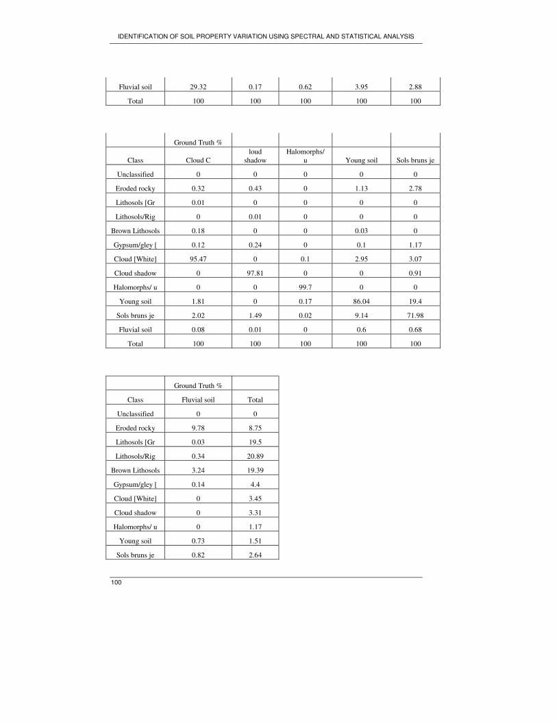
IDENTIFICATION OF SOIL PROPERTY VARIATION USING SPECTRAL AND STATISTICAL ANALYSIS
100
Fluvial soil 29.32 0.17 0.62 3.95 2.88
Total 100 100 100 100 100
Ground Truth %
Class Cloud C
loud
shadow
Halomorphs/
u Young soil Sols bruns je
Unclassified 0 0 0 0 0
Eroded rocky 0.32 0.43 0 1.13 2.78
Lithosols [Gr 0.01 0 0 0 0
Lithosols/Rig 0 0.01 0 0 0
Brown Lithosols 0.18 0 0 0.03 0
Gypsum/gley [ 0.12 0.24 0 0.1 1.17
Cloud [White] 95.47 0 0.1 2.95 3.07
Cloud shadow 0 97.81 0 0 0.91
Halomorphs/ u 0 0 99.7 0 0
Young soil 1.81 0 0.17 86.04 19.4
Sols bruns je 2.02 1.49 0.02 9.14 71.98
Fluvial soil 0.08 0.01 0 0.6 0.68
Total 100 100 100 100 100
Ground Truth %
Class Fluvial soil Total
Unclassified 0 0
Eroded rocky 9.78 8.75
Lithosols [Gr 0.03 19.5
Lithosols/Rig 0.34 20.89
Brown Lithosols 3.24 19.39
Gypsum/gley [ 0.14 4.4
Cloud [White] 0 3.45
Cloud shadow 0 3.31
Halomorphs/ u 0 1.17
Young soil 0.73 1.51
Sols bruns je 0.82 2.64

IDENTIFICATION OF SOIL PROPERTY VARIATION USING SPECTRAL AND STATISTICAL ANALYSIS
101
Fluvial soil 84.93 14.98
Total 100 100
Class Commission Omission Commission Omission
(Percent) (Percent) (Pixels) (Pixels)
Eroded rocky 51.85 65.22 33536/64678 58393/89535
Lithosols [Gr 30.09 16.6 43349/144074 20049/120774
Lithosols/Rig 30.43 13.59 46961/154319 16881/124239
Brown Lithosols 47.32 34.94 67800/143279 40537/116016
Gypsum/gley [ 46.33 85.39 15066/32522 102054/119510
Cloud [White] 12.72 4.53 3240/25463 1054/23277
Cloud shadow 5.25 2.19 1283/24459 518/23694
Halomorphs/ u 0 0.3 0/8676 26/8702
Young soil 53.65 13.96 5973/11133 837/5997
Sols bruns je 31.89 28.02 6229/19534 5180/18485
Fluvial soil 32.03 15.07 35440/110640 13348/88548
Class Prod. Acc. User Acc. Prod. Acc. User Acc.
(Percent) (Percent) (Pixels) (Pixels)
Eroded rocky 34.78 48.15 31142/89535 31142/64678
Lithosols [Gr 83.4 69.91 100725/120774 100725/144074
Lithosols/Rig 86.41 69.57 107358/124239 107358/154319
Brown Lithosols 65.06 52.68 75479/116016 75479/143279
Gypsum/gley [ 14.61 53.67 17456/119510 17456/32522
Cloud [White] 95.47 87.28 22223/23277 22223/25463
Cloud shadow 97.81 94.75 23176/23694 23176/24459
Halomorphs/ u 99.7 100 8676/8702 8676/8676
Young soil 86.04 46.35 5160/5997 5160/11133
Sols bruns je 71.98 68.11 13305/18485 13305/19534
Fluvial soil 84.93 67.97 75200/88548 75200/110640