Identification of Critical Parameters for the Johnson and

MAY 2002 NO. 17

IDENTIFICATION OF CRITICAL PARAMETERS FOR THE JOHNSON AND ETTINGER (1991) VAPOR INTRUSION MODEL

PAUL. C. JOHNSON

DEPARTMENT OF CIVIL AND ENVIRONMENTAL ENGINEERING, ARIZONA STATE UNIVERSITY Executive Summary

At sites where soilpotential for chemical vapbuildings, and other encloextensions (e.g., API Publfor assessing the intrusionmodel, the United States EMicrosoft Excel™ spreads2000). These spreadsheetthe model more accessibleeasier to unknowingly usenumber of inputs, and as awell understood, many usecontributed to confusion a

The objective of threlationships between modwhen applying the model.Johnson and Ettinger (199secondary model inputs anmodel and its implementaapproach for identifying cmodel inputs are discussedcompared with a more tradparametric analysis that is

COPYRIGHT 2002 AMERICAN

A SUMMARY OF RESEARCH RESULTS FROM API’S SOIL & GROUNDWATER TECHNICAL TASK FORCE

s or groundwater contain chemicals of concern, there is the ors to migrate from the subsurface to nearby basements, sed spaces. The Johnson and Ettinger (1991) model and its ication 4674) are at this time the most widely used algorithms of chemical vapors to enclosed spaces. To facilitate use of this nvironmental Protection Agency (USEPA) distributes heets and a comprehensive guidance document (USEPA 1997,

implementations of the model are user-friendly and have made ; however, experience suggests that they have also made it the model inappropriately. The spreadsheets require a large result, relationships between model inputs and outputs are not rs are unable to identify the critical inputs, and this has nd disagreement concerning the utility of the model.

is work is to help users develop a better understanding of the el inputs and outputs so that they can identify critical inputs

This is accomplished by first providing a brief overview of the 1) model, including discussions distinguishing primary and d the differences between the Johnson and Ettinger (1991)

tion in the USEPA spreadsheets. Then, a flowchart-based ritical model inputs is presented and reasonable ranges of . Finally, use of the flowchart approach is illustrated and itional sensitivity analysis. Appendix A presents the

the basis for the flowchart-based approach.

PETROLEUM INSTITUTE

IDENTIFICATION OF CRITICAL PARAMETERS FOR THE JOHNSON AND ETTINGER (1991) VAPOR INTRUSION MODEL MAY 2002 NO. 17

1.0 Introduction

At sites where soils or groundwater contain chemicals of concern, there is the potential for chemical vapors to migrate from the subsurface to nearby basements, buildings, and other enclosed spaces as shown in Figure 1. In extreme cases, these vapors may accumulate at concentrations that pose near-term safety hazards (e.g., explosions or acute health effects) or aesthetic problems (i.e., odors); however, it is more likely that the chemical concentrations will be low, if detectable at all. In the case of lower concentrations the main concern is usually whether or not there is an unacceptable chance of longer-term chronic health effects.

Indoor Air

GroundwaterContamination

Vadose ZoneSoil Gas {SoilContamination(residual ormobile NAPL)

Chemical Vapor Migration

crawl-spaceslab

basement{

Figure 1. Generalized vapor migration-to-indoor-air schematic.

There are three basic options for identifying where this pathway is, and is not a concern. In the first approach, indoor air samples are collected and analyzed, and then the measured concentrations are compared with target indoor air concentrations. In the second approach, available experience and data are compiled and analyzed, and then empirical relationships between site conditions and expected impacts are developed. For example, one might use available data to derive empirical attenuation factors relating subsurface and indoor vapor concentrations, as is done for the Colorado Department of Transportation (CDOT) site in Johnson et al. (2002a). In the third approach, models that consider site conditions (geology, chemical concentrations in soils, vapors, and groundwater, etc.) are used to predict indoor air

COPYRIGHT 2002 AMERICAN PETROLEUM INSTITUTE 1


concentrations. These three approaches need not be mutually exclusive, and each can play a role in some overall integrated framework for assessing potential vapor intrusion impacts (e.g., USEPA 2001).

Because many consider routine indoor air monitoring to be impracticable, and because data from only a few well-studied sites is available (e.g., Johnson et al. 2002a, Hers et al. 2001), the use of screening-level predictive algorithms has played an important role in assessing the significance of this pathway. For example, screening-level algorithms have been used to: • estimate potential indoor impacts at specific sites, • identify sites that require further assessment, • develop chemical- and media-specific target concentrations (e.g., look-up tables) for

identifying settings that are of concern, and • identify how site-specific indoor air concentrations or target soil and groundwater

concentrations are expected to change with changes in site and chemical characteristics

The Johnson and Ettinger (1991) algorithm and its extensions (e.g., Johnson et al. 1998, Johnson et al. 1999) are the most widely used at this time. To facilitate use of the Johnson and Ettinger (1991) model, the United States Environmental Protection Agency (USEPA) distributes Microsoft Excel™ spreadsheets and a comprehensive guidance document (USEPA 1997, 2000). These products are user-friendly and have made the model more accessible; however, experience suggests that they have also made it easier for many to unknowingly use the model inappropriately. The spreadsheets require a large number of inputs, and as a result, relationships between model inputs and outputs are not well understood, many users are unable to identify the critical inputs, and this has contributed to confusion and disagreement concerning the utility of the model. The following may also be contributors: • the USEPA spreadsheets couple other calculations to the Johnson and Ettinger (1991)

algorithm, • most of the Johnson and Ettinger (1991) model inputs are not collected during a typical

site characterization, and therefore, they have to be estimated or inferred from available data and other non-site-specific sources of information, and

• many believe the Johnson and Ettinger (1991) model output to be very sensitive to

uncertainties in model inputs, and therefore feel that the model is of little use until all inputs are known with precision on a site-specific basis.



The objective of this work is to help users develop a better understanding of the

relationships between model inputs and outputs so that they can identify critical inputs when applying the model. This is accomplished by first providing a brief overview of the Johnson and Ettinger (1991) model, including discussions distinguishing primary and secondary model inputs and the differences between the Johnson and Ettinger (1991) model and its implementation in the USEPA spreadsheets. Then, a flowchart-based approach for identifying critical model inputs is presented and reasonable ranges of model inputs are discussed. Finally, use of the flowchart approach is illustrated and compared with a more traditional sensitivity analysis. Appendix A presents the parametric analysis that is the basis for the flowchart-based approach.

It should be noted that this document only addresses use of the Johnson and Ettinger

(1991) model, and this version does not account for biodegradation in the vadose zone. Thus the sensitivity of model results to parameters characterizing biodegradation is not addressed in this document. This issue is addressed in Johnson et al. (1998), Johnson et al. (1999), and Johnson et al. (2002b). In brief, inclusion of biodegradation will result in smaller attenuation factors and decreased indoor air concentrations relative to the case with no biodegradation. Johnson et al. (1998) and Johnson et al (1999) show that the calculations can be extremely sensitive to first-order rate constant changes, when biodegradation is modeled as a simple first order reaction process. In Johnson et al. (2002b), oxygen-limited first-order biodegradation is modeled and those model results are also sensitive to small changes in first-order rate constants. 2.0 Overview of the Johnson and Ettinger (1991) Model and Its USEPA

Spreadsheet Implementation

A brief introduction to the Johnson and Ettinger (1991) algorithm is provided below. The concept of “primary” and “secondary” inputs is introduced and differences between the Johnson and Ettinger (1991) model and its implementation by USEPA in Microsoft Excel™ spreadsheets (1997 – 2001) are identified. 2.1 The Johnson and Ettinger (1991) Algorithm

Screening level algorithms for the vapor intrusion pathway (Johnson and Ettinger 1991, Little et al. 1992, Johnson et al. 1998) couple source zone partitioning, vadose zone transport, building foundation transport, and enclosed-space mixing equations. The resulting algorithms then depend on inputs related to soil, chemical, and building characteristics. The output of the Johnson and Ettinger (1991) algorithm is an estimate of the “vapor attenuation coefficient”



α [dimensionless]. This quantity represents the ratio of the indoor vapor concentration Cindoor to the vapor concentration Csource found at some depth LT below a foundation:

α =

DTeff AB

QB LT

exp

Qsoil LcrackDcrack

eff η AB

expQsoil LcrackDcrack

eff η AB

+

DTeff AB

QB LT

+

DTeff AB

Qsoil LT

exp

Qsoil LcrackDcrack

eff η AB

− 1

(1)

where α=(Cindoor/Csource), and: AB = the surface area of the enclosed space in contact with soil [m2] D = the effective overall vapor-phase diffusion coefficient through the walls and

foundation cracks [mcrackeff

2/d] D = the effective overall vapor-phase diffusion coefficient in soil between the

foundation and the depth LTeff

T [m2/d] Lcrack = the enclosed space foundation thickness [m] LT = the distance (depth) to the vapor source or other point of interest below

foundation [m], measured from the foundation to the vapor source or other point of interest

QB = the enclosed space volumetric air flow rate [m3/d] of fresh air; usually estimated to be the product of the enclosed-space volume (VB [m3]) and the indoor air exchange rate with outdoor air (EB [1/d])

Qsoil = the pressure-driven soil gas flow rate from the subsurface into the enclosed space [m3/d]

η = the fraction of enclosed space surface area open for vapor intrusion [m2/m2]; this is sometimes referred to as the “crack factor” and is estimated to be the total area of cracks, seams, and any perforations of surfaces in contact with soil divided by the total area in contact with soil.

Figure 2 presents the conceptual basis for this algorithm; it also displays the relationship

between the eight primary model inputs and the processes and system components that they characterize.



It should be noted that Equation (1) is the steady-source version of this algorithm. A depleting source form of this equation is also presented in Johnson and Ettinger (1991); however, this document focuses on the steady-source version as it is the most widely used in practice. The use of a steady source term implies an infinite source mass since the chemical concentration at the source never decreases. When the model is to be used for long-term estimation, it is appropriate to perform a reality check by comparing the calculated flux rate with the estimated mass available for volatilization to see if the volatilization rate is sustainable for a reasonable length of time (Johnson et al. 1991, equation 27).

enclosed space

vapormigration

Diffusion[pseudo-

steady state]

Well-Mixed Advection andDiffusion

Source[steady or transient]

VaporSource

DTeff, LT

QBQsoil, AB,

Lcrack, Deffcrack,

η

Figure 2. Johnson and Ettinger (1991) conceptual model showing the primary model inputs and

the processes and system components that they characterize. 2.2 Primary and Secondary Model Inputs

Eight “primary” inputs appear in Equation (1) ( , , QDTeff Dcrack

effsoil, QB, AB, η, Lcrack, LT).

Of these, only LT is likely to be obtained from typical site characterization data. Two others – AB and Lcrack - might easily be measured or at least reasonably estimated based on visual



observation or experience. The remaining inputs (DTeff, Dcrack

eff, Qsoil, QB, and η) must be estimated from knowledge of reasonable ranges for their values, or from expressions relating them to “secondary” inputs that are presumably known.

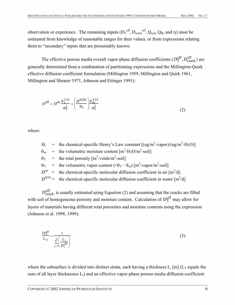
The effective porous media overall vapor-phase diffusion coefficients ( D ,D ) are generally determined from a combination of partitioning expressions and the Millington-Quirk effective diffusion coefficient formulation (Millington 1959, Millington and Quirk 1961, Millington and Shearer 1971, Johnson and Ettinger 1991):

Teff

crackeff

Deff = Dair θv

3.33

θT2

+DH2O

Hi

θm3.33

θT2

(2) where: Hi = the chemical-specific Henry’s Law constant [(ug/m3-vapor)/(ug/m3-H2O)] θm = the volumetric moisture content [m3-H2O/m3-soil] θT = the total porosity [m3-voids/m3-soil] θV = the volumetric vapor content (=θT – θm) [m3-vapor/m3-soil] Dair = the chemical-specific molecular diffusion coefficient in air [m2/d] DH2O = the chemical-specific molecular diffusion coefficient in water [m2/d]

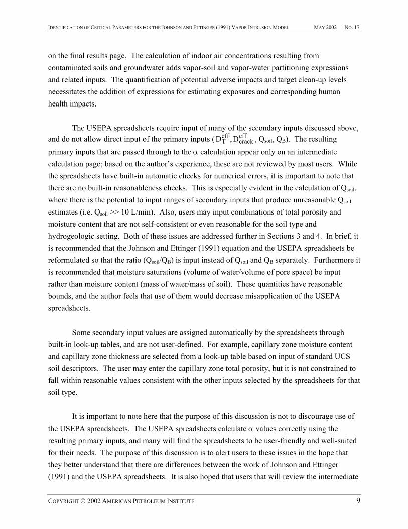
Dcrackeff is usually estimated using Equation (2) and assuming that the cracks are filled

with soil of homogeneous porosity and moisture content. Calculation of may allow for layers of materials having different total porosities and moisture contents using the expression (Johnson et al. 1998, 1999):

DTeff

DTeff

LT=

1Li

Dieff

i=1

n∑

(3)

where the subsurface is divided into distinct strata, each having a thickness Li [m] (LT equals the sum of all layer thicknesses Li) and an effective vapor-phase porous media diffusion coefficient



Dieff [m2/d] calculated using Equation (2) and the layer-specific porosity and moisture content.

For reference, the USEPA spreadsheets allow for three distinct layers. When modeling the flux from groundwater, the capillary zone diffusion resistance is incorporated through Equation 3 by treating the capillary zone as a separate layer. The USEPA spreadsheets estimate Qsoil [m3/s] using the following theoretical expression (Nazaroff 1992):

Qsoil =

2 π k ∆PXcrackµ ln(2Zcrack / Rcrack) (4)

where: k = the soil permeability (near foundation) to air flow [m2] ∆P = the indoor-outdoor pressure difference [g/m-s2] Xcrack = the total length of cracks through which soil gas vapors are flowing [m] µ = the viscosity of air [g/m-s] Zcrack = the crack opening depth below grade [m] Rcrack = the effective crack radius or width (=η AB/Xcrack) [m] This equation is based on the conceptualization that flow to a crack is similar to flow to a cylindrical sink placed at depth Z below grade. Therefore, the soil permeability should reflect the soil properties adjacent to the building. In summary, this development started with the eight primary Johnson and Ettinger (1991) inputs. Most are not typically measured in a site characterization, and therefore empirical and theoretical expressions were introduced for , , and QDcrack

eff DTeff

soil,. In doing this, those three primary inputs were replaced by 12 secondary inputs (HI, [θm, θT]soil, [θm, θT]crack, Dair, DH2O, k, ∆P, Xcrack, µ, and Zcrack). If layered systems are modeled, then the model inputs again increase by three (Li, θm, and θT) for each additional layer. Therefore, the introduction of secondary inputs leads to a substantial increase in the total model inputs. This then makes it very difficult for users to correctly identify relationships between model inputs and output. For all practical purposes, this introduction of secondary



inputs increases the number of unknown inputs; of the new 12 (or more) secondary inputs, the chemical properties (Hi, Dair, DH2O, and µ) are known but the remaining eight (or more) secondary inputs are not normally measured accurately (if at all) in a typical site characterization. 2.3 Key Distinctions Between the Johnson and Ettinger (1991) Model and the USEPA (1997,

2000) Spreadsheet Implementation Since it is not uncommon to have practitioners refer to the USEPA spreadsheets as “The Johnson and Ettinger Model”, it is useful to briefly point out a few key differences between the USEPA spreadsheet implementation and the original Johnson and Ettinger (1991) algorithm. These are summarized below in Table 1. Table 1. Summary of Key Distinctions Between Johnson and Ettinger (1991) and Its USEPA

Spreadsheet Implementation (1997, 2000).

Johnson and Ettinger (1991) USEPA Spreadsheet Implementation (1997, 2000) Output is α, the attenuation factor. Outputs are the incremental risk level, hazard index, or

target soil and groundwater cleanup concentrations for prescribed risk and hazard index. The attenuation factor α is an intermediate calculation not appearing on the final results page.

Qsoil, the pressure-driven soil gas entry flow rate is a user-defined primary input.

Qsoil, the pressure-driven soil gas entry flow rate is an intermediate calculation not appearing on the final results page; it is calculated from user inputs for soil permeability, pressure differential, perimeter crack length, etc..

Capillary zone moisture content and capillary zone thickness are user-defined.

Capillary zone moisture content and capillary zone thickness are assigned through built-in tables for UCS soil descriptors.

The calculation focuses on the ratio of the indoor vapor concentration to the soil gas concentration at some depth.

Soil-to-soil vapor partitioning relationships are introduced; initial spreadsheet implementation limited to single components where immiscible-phase contaminants are not present, although this is not clear to the user.

Common to both is the need to ensure reasonable inputs and consistency between inputs that are expected to be correlated with each other (e.g., total porosity and moisture content in the vadose zone).

First, as stated in the introduction, the Johnson and Ettinger (1991) algorithm is used to estimate the vapor attenuation coefficient. Given the intended audience and their anticipated needs, the USEPA spreadsheets were designed so that the output focuses on predicted indoor air concentrations, incremental risks, hazard quotients, and target risk-based groundwater and soil clean-up levels. The vapor attenuation coefficient α is an intermediate calculation not appearing



on the final results page. The calculation of indoor air concentrations resulting from contaminated soils and groundwater adds vapor-soil and vapor-water partitioning expressions and related inputs. The quantification of potential adverse impacts and target clean-up levels necessitates the addition of expressions for estimating exposures and corresponding human health impacts.

The USEPA spreadsheets require input of many of the secondary inputs discussed above,

and do not allow direct input of the primary inputs ( , , QDTeff Dcrack

effsoil, QB). The resulting

primary inputs that are passed through to the α calculation appear only on an intermediate calculation page; based on the author’s experience, these are not reviewed by most users. While the spreadsheets have built-in automatic checks for numerical errors, it is important to note that there are no built-in reasonableness checks. This is especially evident in the calculation of Qsoil, where there is the potential to input ranges of secondary inputs that produce unreasonable Qsoil estimates (i.e. Qsoil >> 10 L/min). Also, users may input combinations of total porosity and moisture content that are not self-consistent or even reasonable for the soil type and hydrogeologic setting. Both of these issues are addressed further in Sections 3 and 4. In brief, it is recommended that the Johnson and Ettinger (1991) equation and the USEPA spreadsheets be reformulated so that the ratio (Qsoil/QB) is input instead of Qsoil and QB separately. Furthermore it is recommended that moisture saturations (volume of water/volume of pore space) be input rather than moisture content (mass of water/mass of soil). These quantities have reasonable bounds, and the author feels that use of them would decrease misapplication of the USEPA spreadsheets.

Some secondary input values are assigned automatically by the spreadsheets through

built-in look-up tables, and are not user-defined. For example, capillary zone moisture content and capillary zone thickness are selected from a look-up table based on input of standard UCS soil descriptors. The user may enter the capillary zone total porosity, but it is not constrained to fall within reasonable values consistent with the other inputs selected by the spreadsheets for that soil type. It is important to note here that the purpose of this discussion is not to discourage use of the USEPA spreadsheets. The USEPA spreadsheets calculate α values correctly using the resulting primary inputs, and many will find the spreadsheets to be user-friendly and well-suited for their needs. The purpose of this discussion is to alert users to these issues in the hope that they better understand that there are differences between the work of Johnson and Ettinger (1991) and the USEPA spreadsheets. It is also hoped that users that will review the intermediate



spreadsheet calculations (i.e., the primary inputs) to ensure reasonableness in the spreadsheet results. 3.0 A Generalized Approach for Identifying Critical Inputs and Assigning

Reasonable Values of Inputs There are eight primary Johnson and Ettinger (1991) model inputs; with the introduction of secondary inputs, a model application may involve 20 or more inputs. As a result, traditional methods (i.e., sequential variation of individual inputs and inspection of output) are of little use for developing an understanding of the relationships between individual inputs and model output, and for identifying critical model inputs. Appendix A presents an alternate approach, based on a parametric analysis. This approach leads to the conclusion that model output depends only on three basic parameters. It also leads to the conclusion that the dependence of α on individual primary and secondary inputs can be deduced if one understands the relationships between these three parameters and α. The results of the parametric analysis are discussed below and are summarized in the flowchart presented in Figure 3. 3.1 The Three Key Parameters As stated above, the analysis presented in Appendix A leads to the conclusion that model output depends only on three basic parameters:

A =DT

eff

EB (VBAB

) LT

, B =(QsoilQB

) EB (VBAB

) Lcrack

Dcrackeff η

, C =QsoilQB

(5) Readers will note that the parameters A, B, and C appearing in Equation (5) are written in terms of (Qsoil/QB), (VB/AB), η, Lcrack, LT, , , and EDT

eff Dcrackeff

B rather than Qsoil, QB, AB, η, Lcrack, LT, D , and D . This modified set of primary inputs is used because: a) reasonable values T

effcrackeff



for (VB/AB) and EB are constrained to narrow ranges, b) use of the ratio (VB/AB) eliminates the possibility of users assigning inconsistent VB and AB values, c) use of the ratio (Qsoil/QB) eliminates the possibility of users assigning inconsistent Qsoil and QB values, and d) the literature provides more clues for selection of reasonable (Qsoil/QB) ratios than individual Qsoil values. The quantities EB and VB represent the enclosed-space air exchange rate [d-1] and enclosed-space volume [m3], and these are related to QB through the expression: (6) QB = VB EB

3.2 Generalized Flowchart Approach for Identifying Critical Inputs

DTeff Dcrack

effTeff

A generalized flowchart-based approach for identifying critical and non-critical inputs is presented below in Figure 3. For the purposes of this discussion a “non-critical input” is one that can be varied without causing significant changes in the model output (e.g., less than a 20% variation in output across the likely range of values for that input). All other inputs are defined to be “critical inputs”. It is important to note, however, that use of the term “critical” in this context is not meant to imply that large changes in model output are caused by changes in the model inputs. In fact, changes in α are at most linear with changes in primary input values. To use the flowchart, the user begins with reasonable estimates for the primary model inputs, and then calculates values for the parameters A, B, and C. Given these, the user then follows the relevant branch of the flowchart to the list of critical and non-critical primary inputs. Readers will note that there are two branches of the Figure 3 flowchart for which all of the primary inputs are determined to be critical. In these cases, it may be useful to know that α is always bounded such that it will never exceed α=A, as discussed in Appendix A. Thus, the number of critical primary inputs can be reduced from eight {(Qsoil/QB), (VB/AB), η, Lcrack, LT,

, , and EB} to four {(VB/AB), LT, D , and EB} if one is willing to accept a degree of conservatism in the estimated α values. Use of this approach is illustrated in Section 5, where results of the flowchart-based approach are compared with results of a more traditional sensitivity analysis. Before doing that, however, it is important that reasonable ranges for the primary and secondary model inputs be discussed.



Determine Reasonable Initial Estimates for Primary Inputs

{(Qsoil/QB), (VB/AB), η, Lcrack, LT, DeffT, Deff

crack, EB}

Calculate Parameters* {A, B, C}

B<0.1 Other B>3

(AB/C)<0.1

Diffusion is thedominant

mechanism acrossfoundation

Advection is thedominant

mechanism acrossfoundation

Diffusionthrough soilis the over-

all rate-limitingprocess

(AB/C)>10(1+A)Other

Diffusionthrough

foundationis the over-


(A/C)<0.1

Diffusionthrough soilis the over-


(A/C)>10Other

Advectionthrough

foundation isthe over-allrate-limiting

process

Critical Non-Critical

(VB/AB) (Qsoil/QB)LT Lcrack

EB η


(VB/AB) (Qsoil/QB)Lcrack LT

EB

η


(VB/AB) (Qsoil/QB)LT Lcrack

EB η


(Qsoil/QB) (Qsoil/QB)Lcrack

η

LT

EB


(VB/AB) Lcrack

LT

ηEB

(Qsoil/QB)

Result varies with changes in all primaryinputs { (VB/AB), Lcrack, LT, Deff

crack, DeffT,

η. EB, (Qsoil/QB)}; however α is constrainedto be less than A

α ≈A

1+ A

DTeff Dcrack

eff DTeffDcrack

eff DTeff Dcrack

eff Dcrackeff

DTeff

Dcrackeff

DTeff

α ≈CB

α ≈ C

α ≈A

1 + AC

α ≈ A

A =DT

eff

EB ( VBAB

) LT

, B =(Qsoil

QB) EB ( VB

AB) Lcrack

Dcrackeff η

, C =QsoilQB

* ParameterEquations:


Figure 3. Generalized flowchart for identifying critical and non-critical parameters.


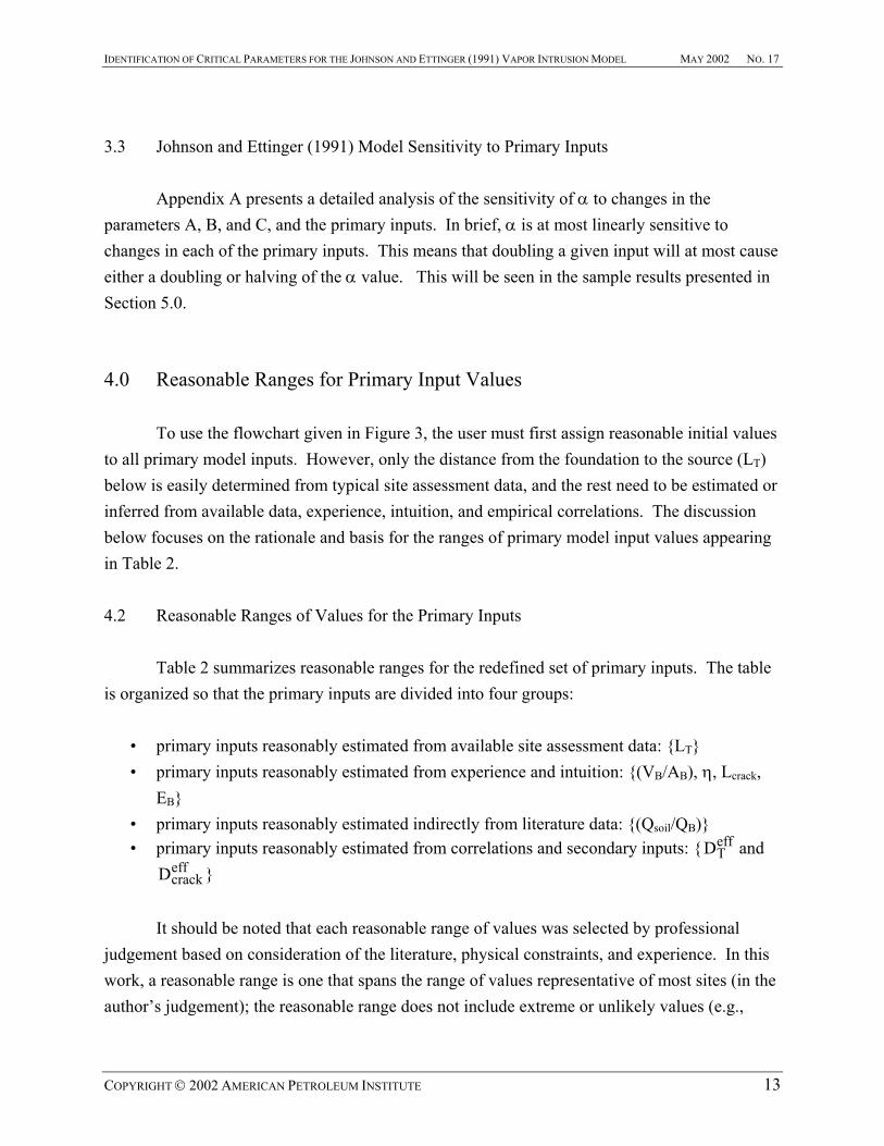
3.3 Johnson and Ettinger (1991) Model Sensitivity to Primary Inputs Appendix A presents a detailed analysis of the sensitivity of α to changes in the parameters A, B, and C, and the primary inputs. In brief, α is at most linearly sensitive to changes in each of the primary inputs. This means that doubling a given input will at most cause either a doubling or halving of the α value. This will be seen in the sample results presented in Section 5.0. 4.0 Reasonable Ranges for Primary Input Values To use the flowchart given in Figure 3, the user must first assign reasonable initial values to all primary model inputs. However, only the distance from the foundation to the source (LT) below is easily determined from typical site assessment data, and the rest need to be estimated or inferred from available data, experience, intuition, and empirical correlations. The discussion below focuses on the rationale and basis for the ranges of primary model input values appearing in Table 2. 4.2 Reasonable Ranges of Values for the Primary Inputs Table 2 summarizes reasonable ranges for the redefined set of primary inputs. The table is organized so that the primary inputs are divided into four groups: • primary inputs reasonably estimated from available site assessment data: {LT} • primary inputs reasonably estimated from experience and intuition: {(VB/AB), η, Lcrack,

EB} • primary inputs reasonably estimated indirectly from literature data: {(Qsoil/QB)} • primary inputs reasonably estimated from correlations and secondary inputs: {D and

} Teff

Dcrackeff

It should be noted that each reasonable range of values was selected by professional judgement based on consideration of the literature, physical constraints, and experience. In this work, a reasonable range is one that spans the range of values representative of most sites (in the author’s judgement); the reasonable range does not include extreme or unlikely values (e.g.,



depth to water of 2000 m). This approach, rather than a statistical data reduction, was used because the available data is limited and comes from a variety of unrelated studies (e.g., the EB Table 2. Summary of Recommendations for Reasonable Primary Input Values. Primary Input

Definition Reasonable Range Comments References

parameters reasonably estimated from available site assessment data LT Depth from foundation to

the vapor source or other point of interest [m]

0.01 – 50 m

To be determined from site assessment data, sampling depths, or defined scenario

Experience

parameters reasonably estimated from experience and intuition (VB/AB) Ratio of enclosed-space

volume to exposed surface area [m]

2 – 3 m

Approximately equal to the height of the enclosed space (e.g., basement height or height of first-floor room for slab-on-grade construction)

Experience

Lcrack Foundation thickness [m] 0.15 – 0.5 m

Based on typical construction practices

Experience

η Fraction of surface area with permeable cracks

0.0005 – 0.005

η=0.01 (worst-case) corresponds to finger-width cracks spaced 1-m apart and running across the floor; η=0.0003 corresponds roughly to a 0.1 cm floor-wall seam perimeter crack around a 225 m2 area

Intuition And (1)

EB Indoor air exchange rate [d-1]

4.8 – 24

Based on building ventilation/energy efficiency studies

(2) – (3)

parameters reasonably estimated indirectly from literature data Qsoil/QB Ratio of the soil gas

intrusion rate to the building ventilation rate

0.05 – 0.0001

Based on vapor attenuation coefficients reported for radon studies and contaminant vapor intrusion case studies

(4) – (8)

parameters reasonably estimated from correlations and secondary inputs DT

eff Effective overall vapor-phase diffusion coefficient between z=LT and the foundation

See Figure 4

Necessary to use empirical correlations and secondary inputs - Equations (2) and (3)

(9) – (11)

Dcrackeff Effective overall vapor-

phase diffusion coefficient through foundation cracks

See Figure 4

Necessary to use empirical correlations and secondary inputs - Equations (2) and (3)

(9) – (11)

(1) - Eaton and Scott (1984); (2) – ASHRAE (1985); (3) Kootz and Rector (1995); (4) - Mose and Mushrush (1999); (5) – Fischer et. al. (1996); (6) – Little et. al. (1992); (7) – Olson and Corsi (2001); (8) – Fitzpatrick and Fitzgerald (1996); (9) – Brooks and Corey (1966); (10) – Carsel and Parish (1988); (11) Johnson and Ettinger (1991); (12) – USEPA (1996).



range comes from a data set on one group of buildings, while (Qsoil/QB) ratios are derived from other studies with other buildings). Reasonable ranges are given here to provide a starting point for input selection, recognizing that appropriate site-specific inputs may fall outside these ranges for a few sites.

4.2.1 Primary Inputs Reasonably Estimated from Available Site Assessment Data {LT} If the Johnson and Ettinger (1991) model is being used to assess impacts at a specific site, then LT is the distance (depth) below a foundation where the soil gas concentration is measured or inferred from another measurement (i.e., dissolved groundwater concentrations). Most values will range between 0.01 and 50 m, with many being concentrated in the 1 to 20 m range. If the model is being used to establish broadly applicable regulatory target levels, it is suggested that users apply the model for a range of LT values (e.g., 0.1 and 10 m). 4.2.2 Primary Inputs Reasonably Estimated from Experience and Intuition: {(VB/AB), η, Lcrack, EB} Three of these inputs {(VB/AB), η, Lcrack} are assigned based on physical intuition, while EB is based on experience recorded in the literature. The inputs {(VB/AB), η, Lcrack} characterize the construction of the enclosed space, which could be a basement or the first-floor of a slab-on-grade construction. (VB/AB) is the ratio of the enclosed-space volume to the exposed surface area; when AB is approximately equal to the enclosed-space footprint then this ratio is equal to the height of the enclosed space. Thus, 2 to 3 m is a reasonable range of values for (VB/AB), and most values will be concentrated in the 2.4 to 2.7 m range. A reasonable range for the foundation thickness (LT) is 0.15 to 0.5 m, with most values being closer to 0.2 m. The parameter η represents the ratio of the area of cracks to the total exposed area (AB). The literature and our experience are of limited use in assigning this value, so we must resort to intuition. Here we imagine a worst-case scenario to be one where parallel 1-cm wide cracks traversing the foundation are spaced every 0.99-m. This scenario corresponds to η=0.01. We can also imagine a scenario where the foundation is relatively crack-free, but vapors can pass through the wall-floor seam. If the wall-floor seam crack is 0.1 cm wide (Eaton and Scott, 1984), then η=0.0008 for a 25 m2 (250 ft2) footprint, η=0.0004 for a 100 m2 (1000 ft2) footprint,



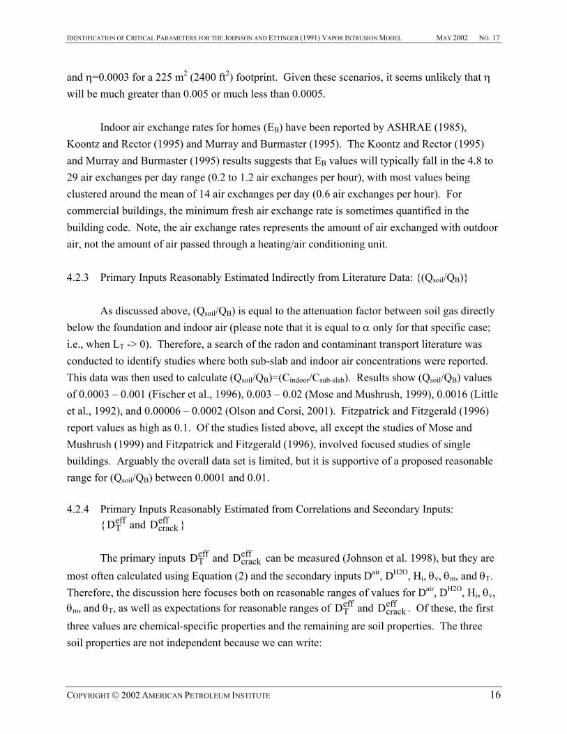
and η=0.0003 for a 225 m2 (2400 ft2) footprint. Given these scenarios, it seems unlikely that η will be much greater than 0.005 or much less than 0.0005. Indoor air exchange rates for homes (EB) have been reported by ASHRAE (1985), Koontz and Rector (1995) and Murray and Burmaster (1995). The Koontz and Rector (1995) and Murray and Burmaster (1995) results suggests that EB values will typically fall in the 4.8 to 29 air exchanges per day range (0.2 to 1.2 air exchanges per hour), with most values being clustered around the mean of 14 air exchanges per day (0.6 air exchanges per hour). For commercial buildings, the minimum fresh air exchange rate is sometimes quantified in the building code. Note, the air exchange rates represents the amount of air exchanged with outdoor air, not the amount of air passed through a heating/air conditioning unit. 4.2.3 Primary Inputs Reasonably Estimated Indirectly from Literature Data: {(Qsoil/QB)}

As discussed above, (Qsoil/QB) is equal to the attenuation factor between soil gas directly below the foundation and indoor air (please note that it is equal to α only for that specific case; i.e., when LT -> 0). Therefore, a search of the radon and contaminant transport literature was conducted to identify studies where both sub-slab and indoor air concentrations were reported. This data was then used to calculate (Qsoil/QB)=(Cindoor/Csub-slab). Results show (Qsoil/QB) values of 0.0003 – 0.001 (Fischer et al., 1996), 0.003 – 0.02 (Mose and Mushrush, 1999), 0.0016 (Little et al., 1992), and 0.00006 – 0.0002 (Olson and Corsi, 2001). Fitzpatrick and Fitzgerald (1996) report values as high as 0.1. Of the studies listed above, all except the studies of Mose and Mushrush (1999) and Fitzpatrick and Fitzgerald (1996), involved focused studies of single buildings. Arguably the overall data set is limited, but it is supportive of a proposed reasonable range for (Qsoil/QB) between 0.0001 and 0.01. 4.2.4 Primary Inputs Reasonably Estimated from Correlations and Secondary Inputs: {D and DT

effcrackeff }

The primary inputs D and DT

effcrackeff can be measured (Johnson et al. 1998), but they are

most often calculated using Equation (2) and the secondary inputs Dair, DH2O, Hi, θv, θm, and θT. Therefore, the discussion here focuses both on reasonable ranges of values for Dair, DH2O, Hi, θv, θm, and θT, as well as expectations for reasonable ranges of D and T

eff Dcrackeff . Of these, the first

three values are chemical-specific properties and the remaining are soil properties. The three soil properties are not independent because we can write:



θv = θT − θm (7)

If Equation (7) is substituted into Equation (2) and rearranged, then:

Deff = Dair θT

1.33[1 − Sm ]3.33{1 +DH 2O

Hi Dair

Sm1 − Sm

3.33} (8)

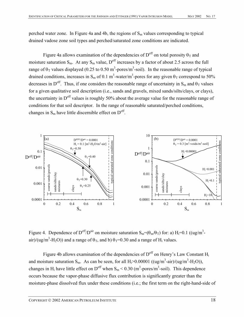
where Sm = (θm/θT) is the moisture saturation. Equation (8) is written in such a way that the secondary inputs are {Dair, θT, Sm, and (DH2O/HiDair)}. This form has been selected for two main reasons – it prevents users from selecting non-physical, or unreasonable combinations of θT, θm, and θv, and also because the second term within the {} on the right-hand side is typically small for transport through the vadose zone. The properties Dair, DH2O, and Hi are chemical-specific and are tabulated for many chemicals in the USEPA spreadsheets. For many chemicals Dair values range from about 0.1 – 1.0 m2/d, DH2O/Dair is usually about 10-4, and Hi values for many aromatics and chlorinated solvents fall in the range 0.01 – 1 ((ug/m3-air)/(ug/m3-H2O)). While diffusion coefficients typically fall within an order-of-magnitude range as indicated above, it is important to note that Henry’s Law Constants range over several orders of magnitude and the range given above is only appropriate for the aromatic and chlorinated solvents considered (e.g., benzene, TCE, etc.). Figure 4 presents the dependence of (Deff/Dair) on θT, Sm, and Hi. In all plots, DH2O/Dair=10-4. In Figure 4a, curves of (Deff/Dair) vs. Sm are presented for Hi=0.1 ((ug/m3-air)/(ug/m3-H2O)) and a range of θT. In Figure 4b, curves of (Deff/Dair) vs. Sm are presented for θT=0.3 and a range of Hi. For reference, typical residual moisture saturations for unconsolidated materials are generally: a) 0.05 – 0.10 for coarse-grained materials like sands and gravels, b) 0.10 - 0.30 for finer-grained mixtures of sands, silts and clays, and c) as high as 0.50 for clayey materials having low proportions of sands and silts (e.g., Carsel and Parrish 1988). Reasonable total porosity values for unconsolidated materials range from about 0.3 [m3-pores/m3-soil] for well-graded/poorly sorted sand, gravel and silt mixtures to about 0.50 [m3-pores/m3-soil] for clays. For a given soil type, the reasonable range of θT and Sm values is relatively narrow (roughly 10% above and below an average value for total porosity and roughly 50% above and below an average value for Sm). It is important to note that these generalizations are specific to well-drained vadose zone materials at residual saturations. Perched water zones, or near-surface soils in high recharge areas may have greater moisture saturations, for example Sm>0.90 for a



perched water zone. In Figure 4a and 4b, the regions of Sm values corresponding to typical drained vadose zone soil types and perched/saturated zone conditions are indicated. Figure 4a allows examination of the dependencies of Deff on total porosity θT and moisture saturation Sm. At any Sm value, Deff increases by a factor of about 2.5 across the full range of θT values displayed (0.25 to 0.50 m3-pores/m3-soil). In the reasonable range of typical drained conditions, increases in Sm of 0.1 m3-water/m3-pores for any given θT correspond to 50% decreases in Deff. Thus, if one considers the reasonable range of uncertainty in Sm and θT values for a given qualitative soil description (i.e., sands and gravels, mixed sands/silts/clays, or clays), the uncertainty in Deff values is roughly 50% about the average value for the reasonable range of conditions for that soil descriptor. In the range of reasonable saturated/perched conditions, changes in Sm have little discernible effect on Deff.

0.0001

0.001

0.01

0.1

1

10

0 0.2 0.4 0.6 0.8 1Sm

Deff/Dair Hi=0.00001

typi

cal s

atur

ated

zon

e co

nditi

onsDH2O/Dair = 0.0001

θT = 0.3 [m3-voids/m3-soil]

Hi=0.001

Hi=0.1

Hi=10

(b)

coar

se sa

nds/

grav

els

sand

s/si

lts/c

lay

mix

ture

s

clay

s

0.0001

0.001

0.01

0.1

1

0 0.2 0.4 0.6 0.8 1Sm

Deff/Dair

θT=0.25

θT=0.30

θT=0.40

θT=0.50

typi

cal s

atur

ated

zon

e co

nditi

ons(a)

coar

se sa

nds/

grav

els

sand

s/si

lts/c

lay

mix

ture

s

clay

s

DH2O/Dair = 0.0001Hi = 0.1 [m3-H2O/m3-air]


Figure 4. Dependence of Deff/Dair on moisture saturation Sm=(θm/θT) for: a) Hi=0.1 ((ug/m3-air)/(ug/m3-H2O)) and a range of θT, and b) θT=0.30 and a range of Hi values. Figure 4b allows examination of the dependencies of Deff on Henry’s Law Constant Hi and moisture saturation Sm. As can be seen, for all Hi>0.00001 ((ug/m3-air)/(ug/m3-H2O)), changes in Hi have little effect on Deff when Sm < 0.30 (m3-pores/m3-soil). This dependence occurs because the vapor-phase diffusive flux contribution is significantly greater than the moisture-phase dissolved flux under these conditions (i.e.; the first term on the right-hand-side of


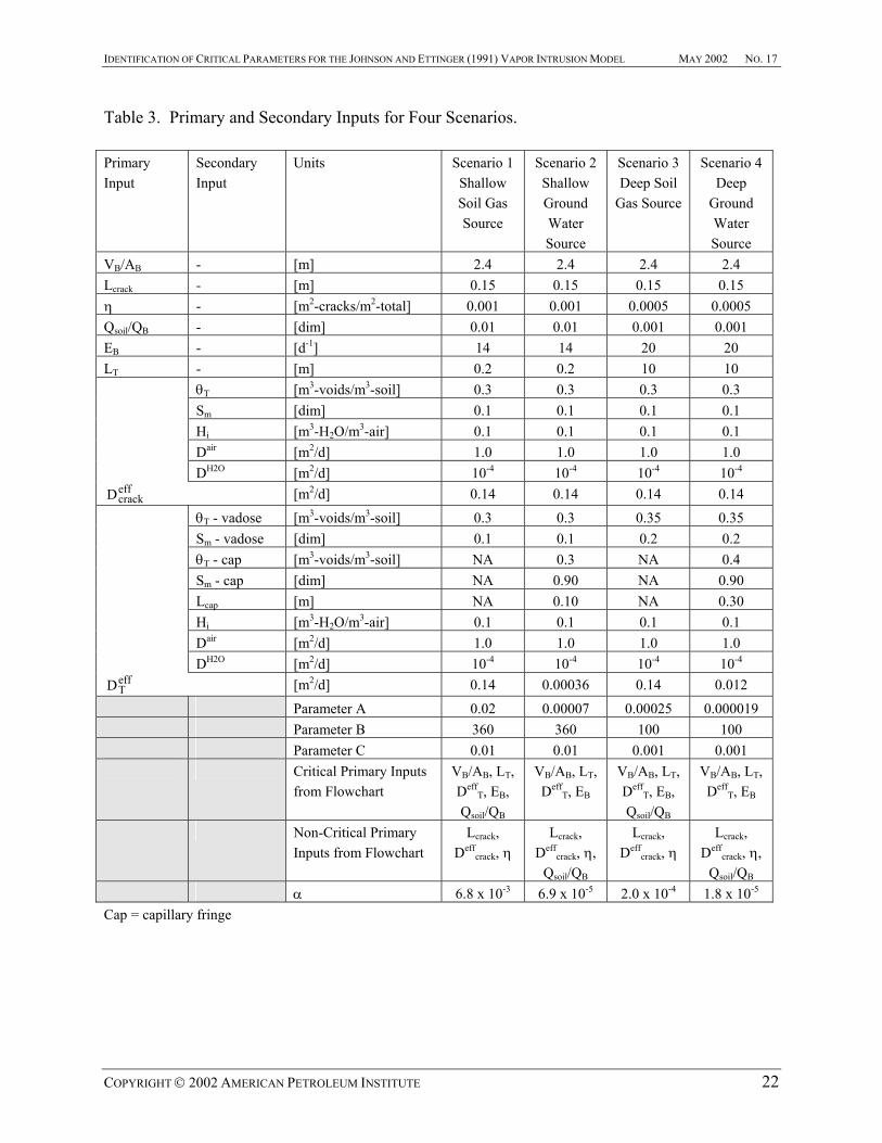
equation (2) is dominant). Changes in Hi have linear effects on Deff in the region typical of saturated conditions (e.g., Deff increases by 10 times when Hi is decreased by a factor of 10). Based on the results given in Figures 4a and 4b, and consideration of Equation (8), the following generalizations can be stated: a) unless Hi < 10-6 ((ug/m3-air)/(ug/m3-H2O)), reasonable Deff ranges for drained vadose zone materials are: a) 0.1Dair to 0.2Dair for coarse sands and gravels, and b) 0.06Dair to 0.2Dair for sand/silt/clay mixtures. For clays at residual saturations in the vadose zone, the reasonable Deff range is 0.02Dair to 0.04Dair, provided that Hi > 0.001 (ug/m3-air)/(ug/m3-H2O). For saturated materials, a reasonable Deff range is 0.2DH2O/Hi to 0.4 DH2O/HI, and these values may be much less than, comparable to, or even greater than the Deff values for vadose conditions as shown in Figure 4b. Some readers may feel that the discussion above is contrary to conventional wisdom, as many practitioners believe Deff to be very sensitive to subtle moisture content changes and that Deff for saturated conditions is always less than Deff for vadose zone conditions. As can be seen in Figure 4, Deff does change significantly across the full range of moisture saturations; however, Deff does not change significantly when constrained to a reasonable range for a given soil descriptor. For example, it would be incorrect to assign a value of Sm=0.50 to coarse sands and gravels in the vadose zone. Also, Deff for near-saturated conditions can be greater than Deff for unsaturated conditions when Hi > 0.00001 ((ug/m3-air)/(ug/m3-H2O)). 5.0 Sample Use of the Figure 3 Flowchart with Reasonable Values of Inputs Table 3 presents primary and secondary inputs for four hypothetical scenarios; two scenarios (1 and 2) represent shallow soil gas and shallow dissolved groundwater source settings and the others (3 and 4) are examples of deep soil gas and deep dissolved groundwater source settings. The parameters A, B, and C are presented for each scenario along with the critical and non-critical primary inputs indicated by the Figure 3 flowchart. In reviewing the parameters, it can be seen that A<<1, B>3, and C<0.01 for all four cases. The Figure 3 flowchart indicates that these are settings in which advection is the dominant mechanism of transport across the foundation (B>3). It also indicates that the primary inputs {Dcrack

eff , Lcrack, and η} are non-critical for the four example settings. To examine if this



conclusion generally holds true, minimum and maximum B values can be calculated for the input ranges given in Table 2. Those B values range roughly from 0.4 to 7 x 104, and this suggests that advection is the dominant mechanism for transport across the foundation for most settings, and that the primary inputs { Dcrack

eff , Lcrack, and η} are non-critical for most settings. This conclusion is consistent with the radon intrusion literature, where advection is believed to be the dominant mechanism for transporting radon across the foundation (Nazaroff 1992). The four example scenarios represent two of the flowchart’s B>3 branches; Scenarios 1 and 3 correspond to 0.1<(A/C)<10, and Scenarios 2 and 4 correspond to (A/C)<0.1. Both branches indicate that (VB/AB), LT, Deff

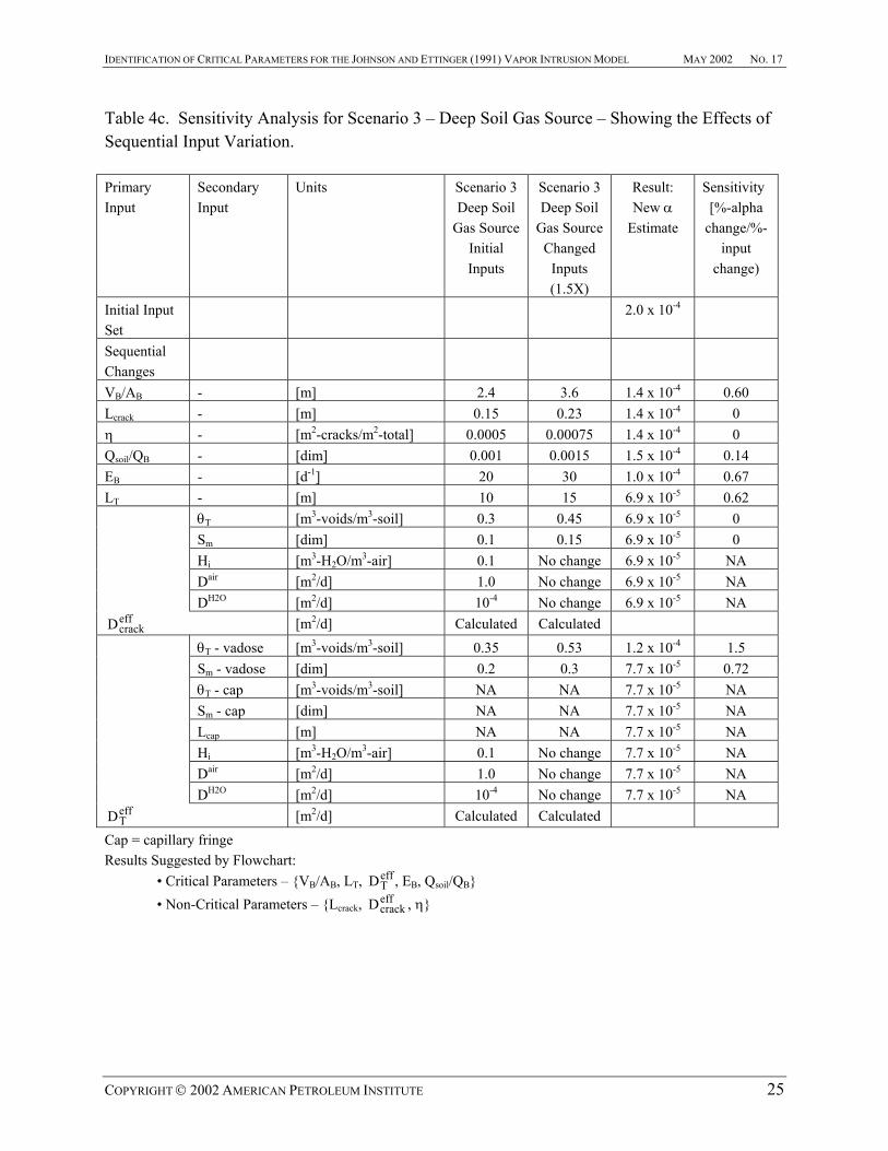
T, and EB could be critical parameters, while the 0.1<(A/C)<10 branch also includes (Qsoil/QB) as a critical input. Again, as discussed previously, variations with changes in these inputs are expected to be at most linear, and this will be tested below. Tables 4a through 4d present results from conventional sensitivity analyses for these four scenarios. The purpose of this exercise is to provide verification that the Figure 3 flowchart provides reasonable results, and also to give the reader an opportunity to see how α varies with sequential changes in inputs. In each case, the effect of sequential 50% increases in input values is examined through changes in vapor attenuation coefficients α. In addition, a normalized measure of sensitivity is presented for each of the inputs. This measure of sensitivity is the ratio of the magnitude of the percentage change in α divided by the magnitude of the percentage change in the input value. For reference, a value of zero indicates that α does not vary with changes in a particular input, and those inputs would be considered to be non-critical. Values close to unity indicate near-linear response within changes in that input. As can be seen, the flowchart identifies the non-critical and critical parameters suggested by the conventional sensitivity analysis. In the cases of Scenarios 2 and 4, the conventional analysis results suggest that α is not sensitive to changes in LT, whereas the flowchart does not indicate this to be a non-critical parameter. Scenarios 2 and 4 correspond to cases where the capillary fringe is the dominant diffusion resistance, and in those cases Deff

T and LT can not be varied independently (see Equation (3)). Under these conditions, Deff

T varies with LT in such a way that the ratio DeffT/LT

changes little as LT changes. Consequently α changes little with variation in LT as α depends on the ratio Deff

T/LT.



In reviewing the sensitivity of model results to changes in inputs for the four cases, it can be seen that changes in output with changes in input is often approximately linear (e.g., the sensitivity measure is approximately unity), and that the sensitivity is low to changes in most parameter values. Again, this illustrates that, contrary to some practitioners beliefs, the Johnson and Ettinger (1991) model output is generally affected by only a small number of inputs, provided that inputs are varied across reasonable ranges of values. The results also show that use of the flowchart-based approach leads to reliable identification of non-critical inputs and potentially critical inputs. Generally, the results in Tables 4a through 4d suggest that the non-critical inputs identified by Figure 3 are indeed non-critical, and that the actual number of critical inputs may be less than that suggested by Figure 3. 6.0 Summary It is difficult for users to develop a thorough understanding of the relationships between model inputs and outputs so that they can identify critical inputs when applying the Johnson and Ettinger (1991) model or when using the USEPA spreadsheet implementation of this model. The parametric analysis conducted above shows that model output is controlled by three dimensionless parameters, and that if one understands how output varies with changes in these parameters, then the dependence on individual inputs can also be correctly deduced. The results also show that the sets of critical and non-critical inputs are not fixed, but that they are dictated by the specific combination of the three parameters. Thus, a spreadsheet approach can help users identify the critical and non-critical inputs for each application. Reasonable ranges for the primary inputs are also tabulated here to provide users a basis for comparison with their input sets. Sample use of the flowchart for four scenarios suggests that some inputs are non-critical for most applications. Use of the four scenarios also shows that the simplified flowchart approach leads to the same conclusions as a more lengthy and complex conventional sensitivity analysis.



Table 3. Primary and Secondary Inputs for Four Scenarios. Primary Input

Secondary Input

Units Scenario 1 Shallow Soil Gas Source

Scenario 2 Shallow Ground Water Source

Scenario 3 Deep Soil

Gas Source

Scenario 4 Deep

Ground Water Source

VB/AB - [m] 2.4 2.4 2.4 2.4 Lcrack - [m] 0.15 0.15 0.15 0.15 η - [m2-cracks/m2-total] 0.001 0.001 0.0005 0.0005 Qsoil/QB - [dim] 0.01 0.01 0.001 0.001 EB - [d-1] 14 14 20 20 LT - [m] 0.2 0.2 10 10 θT [m3-voids/m3-soil] 0.3 0.3 0.3 0.3 Sm [dim] 0.1 0.1 0.1 0.1 Hi [m3-H2O/m3-air] 0.1 0.1 0.1 0.1 Dair [m2/d] 1.0 1.0 1.0 1.0 DH2O [m2/d] 10-4 10-4 10-4 10-4 Dcrack

eff [m2/d] 0.14 0.14 0.14 0.14

θT - vadose [m3-voids/m3-soil] 0.3 0.3 0.35 0.35 Sm - vadose [dim] 0.1 0.1 0.2 0.2 θT - cap [m3-voids/m3-soil] NA 0.3 NA 0.4 Sm - cap [dim] NA 0.90 NA 0.90 Lcap [m] NA 0.10 NA 0.30 Hi [m3-H2O/m3-air] 0.1 0.1 0.1 0.1 Dair [m2/d] 1.0 1.0 1.0 1.0 DH2O [m2/d] 10-4 10-4 10-4 10-4 DT

eff [m2/d] 0.14 0.00036 0.14 0.012

Parameter A 0.02 0.00007 0.00025 0.000019 Parameter B 360 360 100 100 Parameter C 0.01 0.01 0.001 0.001 Critical Primary Inputs

from Flowchart VB/AB, LT, Deff

T, EB, Qsoil/QB

VB/AB, LT, Deff

T, EB VB/AB, LT, Deff

T, EB, Qsoil/QB

VB/AB, LT, Deff

T, EB

Non-Critical Primary Inputs from Flowchart

Lcrack, Deff

crack, η Lcrack,

Deffcrack, η,

Qsoil/QB

Lcrack, Deff

crack, η Lcrack,

Deffcrack, η,

Qsoil/QB α 6.8 x 10-3 6.9 x 10-5 2.0 x 10-4 1.8 x 10-5 Cap = capillary fringe



Table 4a. Sensitivity Analysis for Scenario 1 – Shallow Soil Gas Source – Showing the Effects of Sequential Input Variation. Primary Input

Secondary Input

Units Scenario 1 Shallow Soil Gas Source Initial Inputs

Scenario 1 Shallow Soil Gas Source

Changed Inputs (1.5X)

Result: New α

Estimate

Sensitivity [%-alpha

change/%-input

change)

Initial Input Set

6.8 x 10-3

Sequential Changes

VB/AB - [m] 2.4 3.6 5.9 x 10-3 0.29 Lcrack - [m] 0.15 0.23 5.9 x 10-3 0 η - [m2-cracks/m2-total] 0.001 0.0015 5.9 x 10-3 0 Qsoil/QB - [dim] 0.01 0.015 7.3 x 10-3 0.48 EB - [d-1] 14 21 5.8 x 10-3 0.41 LT - [m] 0.2 0.3 4.4 x 10-3 0.47 θT [m3-voids/m3-soil] 0.3 0.45 4.4 x 10-3 0 Sm [dim] 0.1 0.15 4.4 x 10-3 0 Hi [m3-H2O/m3-air] 0.1 No change 4.4 x 10-3 NA Dair [m2/d] 1.0 No change 4.4 x 10-3 NA DH2O [m2/d] 10-4 No change 4.4 x 10-3 NA Dcrack

eff [m2/d] Calculated Calculated

θT - vadose [m3-voids/m3-soil] 0.3 0.45 6.3 x 10-3 0.83 Sm - vadose [dim] 0.1 0.15 5.9 x 10-3 0.22 θT - cap [m3-voids/m3-soil] NA No change 5.9 x 10-3 NA Sm - cap [dim] NA No change 5.9 x 10-3 NA Lcap [m] NA No change 5.9 x 10-3 NA Hi [m3-H2O/m3-air] 0.1 No change 5.9 x 10-3 NA Dair [m2/d] 1.0 No change 5.9 x 10-3 NA DH2O [m2/d] 10-4 No change 5.9 x 10-3 NA DT


Cap = capillary fringe Results Suggested by Flowchart: • Critical Parameters – {VB/AB, LT, , EDT

effB, Qsoil/QB}

• Non-Critical Parameters – {Lcrack, Dcrackeff , η}



Table 4b. Sensitivity Analysis for Scenario 2 – Shallow Groundwater Source – Showing the Effects of Sequential Input Variation. Primary Input

Secondary Input

Units Scenario 2 Shallow Ground Water Source Initial Inputs

Scenario 2 Shallow Ground Water Source


Result: New α

Estimate


change/%-input

change)

Initial Input Set

6.9 x 10-5

Sequential Changes

VB/AB - [m] 2.4 3.6 4.7 x 10-5 0.64 Lcrack - [m] 0.15 0.23 4.7 x 10-5 0 η - [m2-cracks/m2-total] 0.001 0.0015 4.7 x 10-5 0 Qsoil/QB - [dim] 0.01 0.015 4.7 x 10-5 0 EB - [d-1] 14 21 3.1 x 10-5 0.68 LT - [m] 0.2 0.3 3.1 x 10-5 0 θT [m3-voids/m3-soil] 0.3 0.45 3.1 x 10-5 0 Sm [dim] 0.1 0.15 3.1 x 10-5 0 Hi [m3-H2O/m3-air] 0.1 No change 3.1 x 10-5 NA Dair [m2/d] 1.0 No change 3.1 x 10-5 NA DH2O [m2/d] 10-4 No change 3.1 x 10-5 NA Dcrack


θT - vadose [m3-voids/m3-soil] 0.3 0.45 3.1 x 10-5 0 Sm - vadose [dim] 0.1 0.15 3.1 x 10-5 0 θT - cap [m3-voids/m3-soil] 0.3 0.45 5.3 x 10-5 1.4 Sm - cap [dim] 0.90 0.99 4.4 x 10-5 1.7 Lcap [m] 0.1 0.15 2.9 x 10-5 0.66 Hi [m3-H2O/m3-air] 0.1 No change 2.9 x 10-5 NA Dair [m2/d] 1.0 No change 2.9 x 10-5 NA DH2O [m2/d] 10-4 No change 2.9 x 10-5 NA DT



effB}

• Non-Critical Parameters – {Lcrack, Dcrackeff , η, Qsoil/QB}



Table 4c. Sensitivity Analysis for Scenario 3 – Deep Soil Gas Source – Showing the Effects of Sequential Input Variation. Primary Input

Secondary Input

Units Scenario 3 Deep Soil

Gas Source Initial Inputs

Scenario 3 Deep Soil

Gas Source Changed

Inputs (1.5X)

Result: New α

Estimate


change/%-input

change)

Initial Input Set

2.0 x 10-4

Sequential Changes

VB/AB - [m] 2.4 3.6 1.4 x 10-4 0.60 Lcrack - [m] 0.15 0.23 1.4 x 10-4 0 η - [m2-cracks/m2-total] 0.0005 0.00075 1.4 x 10-4 0 Qsoil/QB - [dim] 0.001 0.0015 1.5 x 10-4 0.14 EB - [d-1] 20 30 1.0 x 10-4 0.67 LT - [m] 10 15 6.9 x 10-5 0.62 θT [m3-voids/m3-soil] 0.3 0.45 6.9 x 10-5 0 Sm [dim] 0.1 0.15 6.9 x 10-5 0 Hi [m3-H2O/m3-air] 0.1 No change 6.9 x 10-5 NA Dair [m2/d] 1.0 No change 6.9 x 10-5 NA DH2O [m2/d] 10-4 No change 6.9 x 10-5 NA Dcrack


θT - vadose [m3-voids/m3-soil] 0.35 0.53 1.2 x 10-4 1.5 Sm - vadose [dim] 0.2 0.3 7.7 x 10-5 0.72 θT - cap [m3-voids/m3-soil] NA NA 7.7 x 10-5 NA Sm - cap [dim] NA NA 7.7 x 10-5 NA Lcap [m] NA NA 7.7 x 10-5 NA Hi [m3-H2O/m3-air] 0.1 No change 7.7 x 10-5 NA Dair [m2/d] 1.0 No change 7.7 x 10-5 NA DH2O [m2/d] 10-4 No change 7.7 x 10-5 NA DT



effB, Qsoil/QB}

• Non-Critical Parameters – {Lcrack, Dcrackeff , η}



Table 4d. Sensitivity Analysis for Scenario 4 – Deep Groundwater Source – Showing the Effects of Sequential Input Variation. Primary Input

Secondary Input

Units Scenario 4 Deep

Ground Water Source Initial Inputs

Scenario 4 Deep

Ground Water Source


Result: New α

Estimate


change/%-input

change)

Initial Input Set

1.8 x 10-5

Sequential Changes

VB/AB - [m] 2.4 3.6 1.2 x 10-5 0.67 Lcrack - [m] 0.15 0.23 1.2 x 10-5 0 η - [m2-cracks/m2-total] 0.0005 0.00075 1.2 x 10-5 0 Qsoil/QB - [dim] 0.001 0.0015 1.2 x 10-5 0 EB - [d-1] 20 30 8.3 x 10-6 0.62 LT - [m] 10 15 8.0 x 10-6 0.075 θT [m3-voids/m3-soil] 0.3 0.45 8.0 x 10-6 0 Sm [dim] 0.1 0.15 8.0 x 10-6 0 Hi [m3-H2O/m3-air] 0.1 No change 8.0 x 10-6 NA Dair [m2/d] 1.0 No change 8.0 x 10-6 NA DH2O [m2/d] 10-4 No change 8.0 x 10-6 NA Dcrack


θT - vadose [m3-voids/m3-soil] 0.35 0.53 8.3 x 10-6 0.075 Sm - vadose [dim] 0.2 0.3 8.0 x 10-6 0.075 θT - cap [m3-voids/m3-soil] 0.35 0.53 1.3 x 10-5 1.25 Sm - cap [dim] 0.90 0.99 1.1 x 10-5 0.31 Lcap [m] 0.3 0.45 7.7 x 10-6 0.6 Hi [m3-H2O/m3-air] 0.1 No change 7.7 x 10-6 NA Dair [m2/d] 1.0 No change 7.7 x 10-6 NA DH2O [m2/d] 10-4 No change 7.7 x 10-6 NA DT



effB}

• Non-Critical Parameters – {Lcrack, Dcrackeff , η, Qsoil/QB}



References American Society of Heating Refrigerating and Air Conditioning Engineers (ASHRAE). 1985. ASHRAE Handbook (1985) Fundamentals. Chapter 22. Atlanta, GA. Brooks, R.H. and Corey. 1966. Properties of Porous Media Affecting Fluid Flow. ASCE J. Irrig. Drainage Div.. 72(IR2), 61-88. Carsel, R.F. and R.S. Parrish. 1988. Developing Joint Probability Distributions of Soil Water Retention Characteristcs. Water Resources Research. 24(5). 755-769. Eaton, R.S. and A.G. Scott. 1984. Understanding Radon Transport Into Houses. Radiation Protection Dosimetry. 7. 251-253. Fischer, M.L., A.J. Bentley, K.A. Dunkin, A.T. Hodgson, W.W. Nazaroff, R.G. Sextro, and J.M. Daisey. 1996. Factors Affecting Indoor Air Concentrations of Volatile Organic Compounds at a Site of Subsurface Gasoline Contamination. Environ. Sci. Technol.. 30 (10). 2948-2957 Fitzpatrick, N.A. and J.J. Fitzgerald. 1996. An Evaluation of Vapor Intrusion Into Buildings Through a Study of Field Data. Presented at the 11th Annual Conference on Contaminated Soils. University of Massachusetts – Amherst. October. Hers, I., R. Zapfe-Gilje, L. Li, and J. Atwater. 2001. The Use of Indoor Air Measurements to Evaluate Intrusion of Subsurface VOC Vapors into Buildings. J. Air & Waste Manage. Assoc.. 51. 1318-1331. Hers, I., R. Zapf-Gilje, P. C. Johnson, and L. Li. 2002. Evaluation of the Johnson and Ettinger Model for Prediction of Indoor Air Quality. Accepted for publication in Ground Water Monitoring and Remediation. Johnson, P.C. and R.A. Ettinger. 1991. Heuristic Model for Predicting the Intrusion Rate of Contaminant Vapors Into Buildings. Environ. Sci. Technol.. 25. 1445-1452. Johnson, P.C., C. Bruce. R.L. Johnson, and M.W. Kemblowski. 1998. In Situ Measurement of Effective Vapor-Phase Porous Medium Diffusion Coefficients. Environmental Science and Technology. 32. 3405-3409. Johnson, P.C., R.L. Johnson, and M.W. Kemblowski. 1998. Assessing the Significance of Subsurface Contaminant Migration to Enclosed Spaces: Site-Specific Alternatives to Generic Estimates. American Petroleum Institute Publication No. 4674. December.



Johnson, P.C., R.L. Johnson, and M.W. Kemblowski. 1999. Assessing the Significance of Vapor Migration to Enclosed-Spaces on a Site-Specific Basis. Journal of Soil Contamination. 8 (3). 389 - 421. Johnson, P.C., R.A. Ettinger, J. Kurtz, R. Bryan, and J.E. Kester. 2002a. Migration of Soil Gas Vapors to Indoor Air: Determining Vapor Attenuation Factors Using a Screening-Level Model and Field Data from the CDOT-MTL Denver, Colorado Site. American Petroleum Institute Bulletin No.16. April. Johnson, P. C., V. A. Hermes, S. Roggemans. 2002b. An Oxygen-Limited Hydrocarbon Vapor Migration Attenuation Screening Model. In preparation. Koontz, M.D. and H.E. Rector. 1995. Estimation of Distributions for Residential Air Exchange Rates. EPA Contract No. 68-D9-0166, Work Assignment No. 3-19. USEPA Office of Pollution Prevention and Toxics. Washington, D.C. Little, J.C., J.M. Daisey, W.W. Nazaroff. 1992. Transport of Subsurface Contaminants into Buildings: An Exposure Pathway for Volatile Organics. Environ. Sci. Technol.. 26. 2058-2066.

Millington, R. J., Gas Diffusion in Porous Media, Science, 1959, 130, 100-102. Millington, R. J. and J. P. Quirk,. 1961. Permeability of Porous Solids, Trans. Faraday Soc.. 57. 1200-1207. Millington, R. J. and R. C. Shearer. 1971. Diffusion in Aggregated Porous Media, Soil Sci.. 111. 372-378. Murray, D.M. and D.E. Burmaster. 1995. Residential Air Exchange Rates in the United States: Empirical and Estimated Parametric Distributions by Season and Climactic Region. Risk Analysis. 15. 459-465. Mose, D.G. and G.W. Mushrush. 1999. Comparisons Between Soil Radon and Indoor Radon. Energy Sources. 21. 723-731. Nazaroff, W.W.. 1992. Radon Transport from Soil to Air. Review of Geophysics. 30 (2). 137 – 160.



Olson, D.A. and R.L. Corsi. 2001. Characterizing Exposure to Chemicals from Soil Vapor Intrusion Using a Two-Compartment Model. Atmospheric Environment. 35. 4201-4209. Robinson, A.L., R.G. Sextro, W.J. Fisk. 1997. Soil-Gas Entry Into an Experimental Basement Driven by Atmospheric Pressure Fluctuations – Measurements, Spectral Analysis, and Model Comparison. Atmospheric Environment. 31 (10). 1477-1485. Robinson, A.L. and R.G. Sextro. 1997. Radon Entry into Buildings Driven by Atmospheric Pressure Fluctuations. Environ. Sci. Technol.. 31 (6). 1742-1748. USEPA. 1997. User’s Guide for the Johnson and Ettinger (1991) Model for Subsurface Vapor Intrusion Into Buildings. Prepared by Environmental Quality Management, Inc.. Contract No. 68-D30035. September 1997. [http://www.epa.gov/superfund/programs/risk/airmodel/johnson_ettinger.htm] USEPA. 1997 - 2000. Spreadsheets for the Johnson and Ettinger (1991) Model. Prepared by Environmental Quality Management, Inc.. [http://www.epa.gov/superfund/programs/risk/airmodel/johnson_ettinger.htm] USEPA. 2001. Draft Supplemental Guidance for Evaluating the Vapor Intrusion to Indoor Air Pathway. November.



Appendix A: Understanding Relationships Between Model Inputs and α-Values, and the Identification of Critical and Non-Critical Primary Inputs

There are eight primary Johnson and Ettinger (1991) model inputs; with the introduction of secondary inputs, a model application may involve 20 or more inputs. Therefore, it is unlikely that traditional methods (i.e., sequential variation of individual inputs and inspection of output) will be of use for developing an understanding of the relationships between individual inputs and model output. A parametric analysis of the Johnson and Ettinger (1991) equation is conducted below. It will be shown that model output depends on only three basic parameters. These “parameters” are dimensionless groupings of the primary inputs. Furthermore it will be shown that these parameters have physical relevance and the dependence of α on individual primary and secondary inputs can easily be deduced if one understands the relationships between these parameters and α. The results of this parametric analysis were used to create the flowchart-based approach presented in Figure 3 of the main body of this report. That figure presents a generalized approach for identifying the critical and non-critical model inputs. For the purposes of this discussion a “non-critical input” is one that can be varied without causing significant changes in the model output (e.g., less than a 20% variation in output across the likely range of values for that input). All other inputs are defined to be “critical inputs”. It is important to note, however, that use of the term “critical” in this context is not meant to imply that large changes in model output are caused by small changes in the model inputs. In fact, it will be seen that changes in α are at most linear with changes in primary input values. A.1 Parametric Analysis of the Johnson and Ettinger (1991) Algorithm While the Johnson and Ettinger (1991) algorithm is often written in terms of eight primary inputs, it can also be written much more simply in terms of three dimensionless parameters:

α =A[ ]exp B( )

exp B( )+ A[ ]+AC

exp B( )− 1( )

(A1)

COPYRIGHT 2002 AMERICAN PETROLEUM INSTITUTE A1


where:

A =DT

eff ABQB LT

, B =

Qsoil Lcrack

Dcrackeff η AB

, C =QsoilQB

(A2) or:

A =DT

eff

EB (VBAB

) LT

, B =(QsoilQB

) EB (VBAB

) Lcrack

Dcrackeff η

, C =QsoilQB

(A3) and: AB = the surface area of the enclosed space in contact with soil [m2] α = (Cindoor/Csource); Cindoor denotes the indoor air concentration and Csource is the

vapor concentration at some depth (both in consistent units) D = the effective overall vapor-phase diffusion coefficient through the walls and


2/d] D = the effective overall vapor-phase diffusion coefficient between the foundation

and the depth LTeff

T [m2/d] Lcrack = the enclosed space foundation thickness [m] LT = the distance (depth) to the vapor source or other point of interest below

foundation [m] QB = the enclosed space volumetric air flow rate [m3/d]; usually estimated to be the

product of the enclosed-space volume (VB [m3]) and the indoor air exchange rate (EB [1/d])


η = the fraction of enclosed space surface area open for vapor intrusion [m2/m2]; this is sometimes referred to as the “crack factor” and is estimated to be the total area of cracks, seams, and any perforations of surfaces in contact with soil divided by the total area in contact with soil.

This parametric form of the Johnson and Ettinger (1991) algorithm provides a valuable tool for developing an understanding of the relationships between model inputs and α. If one



can understand the relationships between these three parameters and the model output, then the dependence on individual primary or secondary inputs can be deduced. It is useful to note that each of the parameters has physical relevance: • A (= D AT

effB/QB LT) is equal to the vapor attenuation coefficient for cases where

there is no foundation (e.g., a bare dirt floor) and diffusion through the soil to the foundation is the controlling mechanism.

• B (=Qsoil Lcrack/ ADcrack

effB η) is a measure of the significance of the two mechanisms

responsible for transporting chemical vapors across the building foundation (advection and diffusion). If B>>1 then advection is primarily responsible for chemical transport across the foundation; if B<<1, then diffusion is primarily responsible for chemical transport across the foundation.

• C (=Qsoil/QB) is equal to the vapor attenuation coefficient between vapors

immediately below the foundation and indoor air (e.g., LT-->0), provided that advection is the mechanism responsible for transport across the foundation (i.e., B>>1).

In addition, combinations of these parameters also have physical relevance: • The combination (AB/C) (= D LT

effcrack/LT η) is a measure of the significance

of diffusive transport through the soil relative to diffusive transport through the foundation. As shown below, it appears in Equation A4 when B<<1. If (AB/C)>>1 then diffusion through the foundation is the overall rate-limiting process; if (AB/C)<<1 then diffusion through the soil is the overall rate-limiting process.

Dcrackeff

• The combination (B/C) (=QB Lcrack/AB η) is equal to the vapor attenuation

coefficient between vapors immediately below the foundation and indoor air (e.g., L

Dcrackeff

T-->0), provided that diffusion through the foundation is the mechanism responsible for transport across the foundation (i.e., B<<1). It appears in Equation A4 when B<<1 and (AB/C)>10(1+A).

Figure A1 presents a series of four graphs that illustrate the dependence of α on the three parameters A, B, and C. Each graph plots α as a function of A over the range 10-5≤A≤1 for a



range of C values (C=0.0001, 0.001, and 0.01); each graph was also prepared using a different B value (B=0.001, 0.1, 1, and 10). These ranges of values were selected based on consideration of the discussion of reasonable ranges of primary inputs given in Section 4. In the following discussion, mathematical analysis supported by these graphs is used to determine the dependence of α on the primary inputs.

A

B = 0.001 B = 0.1

B = 1 B = 10

α α

α α

C = 0.01

C = 0.001

C = 0.0001

C = 0.01

C = 0.001

C = 0.0001

C = 0.01

C = 0.001

C = 0.0001

C = 0.01

C = 0.001

C = 0.0001

A

A A

1.E-05

1.E-04

1.E-03

1.E-02

1.E-01

1.E-05 1.E-04 1.E-03 1.E-02 1.E-01 1.E+001.E-05

1.E-04

1.E-03

1.E-02

1.E-01

1.E-05 1.E-04 1.E-03 1.E-02 1.E-01 1.E+00

1.E-05

1.E-04

1.E-03

1.E-02

1.E-01

1.E-05 1.E-04 1.E-03 1.E-02 1.E-01 1.E+001.E-05

1.E-04

1.E-03

1.E-02

1.E-01

1.E-05 1.E-04 1.E-03 1.E-02 1.E-01 1.E+00

Figure A1. Variation in α with changes in the parameters A, B, and C.



Thus, the B=0.001 plot corresponds to the case where diffusion is the dominant transport mechanism through the foundation. Mathematically, when B<0.1, Equation (A1) can be approximated by:

α =A[ ]

1+ A[ ]+AC

B( )

, B < 0.1

(A4) Provided that (AB/C)<0.1, it is expected that α should vary only with A:

α =

A[ ]1+ A[ ] , B < 0.1 and

A BC

< 0.1 (A5)

This behavior is seen with decreasing A in the B=0.001 and B=0.1 plots (note that α=A for A<<1). Physically, this condition (B<0.1 and AB/C<0.1) corresponds to cases where diffusion through soil is the overall rate-limiting transport mechanism. Consequently, α varies only with changes in A, so that D , AT

effB, QB, and LT (and any related secondary inputs) are the only

critical inputs. The B=0.001 curves also show that changes in α with respect to changes in , A

DTeff

B, QB, and LT are at most linear (e.g., increasing LT by a factor of two decreases α by 1/2, increasing D by a factor of two increases α by a factor 2). T

eff

If B<0.1 and (AB/C)>10(1+A), then:

α =

C[ ]B[ ] , B < 0.1and

A BC

> 10(1+ A) (A6)

This behavior is seen in the asymptotes of the B=0.1 curves as A increases. Physically, this condition (B<0.1 and AB/C>10(1+A)) corresponds to cases where diffusion through the foundation is the overall rate-limiting transport mechanism. Under these conditions α varies only with changes in the ratio (C/B), so that , ADcrack

effB, QB, η, and Lcrack (and any related

secondary inputs) are the only critical inputs. The B=0.1 curves also show that changes in α with respect to changes in these parameters are at most linear.



The B=10 plot corresponds to the case where advection is the dominant transport mechanism across the foundation. Mathematically, when B>3, then exp(B)>10 and Equation (A1) reduces to:

α =A[ ]

1+AC

, B> 3

(A7) Therefore, α is expected to be independent of B for B>3, and this can be seen by comparing the curves in the B=1 and B=10 plots. The vapor attenuation coefficient α is dependent only on those inputs affecting the values of A and C. Thus, Lcrack, D , and η are non-critical inputs under these conditions. Again, the B=1 and B=10 graphs show that the sensitivity of α to changes in the primary inputs appearing in A and C is at most linear, and under the conditions discussed below, some other inputs may also be non-critical.

crackeff

If in addition to the condition B>3, advective transport across the building foundation is the overall limiting transport mechanism between the point of interest (LT) and the enclosed space, then (A/C)>10 and:

α = C , B> 3 and

AC

> 10 (A8)

This limit is observed in Figure A1 as all α-vs-A curves asymptote with increasing A to α=C for B=1 and B=10. This condition is most likely to be met when assessing the attenuation between soil gas immediately below a foundation and indoor air (LT-->0). Under these conditions, we need only know Qsoil and QB (or the ratio Qsoil/QB) to estimate α. Sensitivity of α to changes in Qsoil and QB is linear in Equation (A8). If B>3 and transport through the vadose zone is the limiting transport mechanism between the point of interest (LT) and the enclosed space, then (A/C)<0.1, and:

α = A, B > 3 and

AC

< 0.1 (A9)

This limit is observed in Figure A1 as all α-vs-A curves asymptote with decreasing A to α=A for B=1 and B=10. This condition is most likely to be met when we are interested in assessing the



attenuation between soil gas located more than a few meters below a foundation, or possibly the attenuation of vapors originating from dissolved groundwater contamination. Under these conditions, we need only know , ADT

effB, QB, and LT to estimate α.



Basic Nomenclature A, B, C = dimensionless parameters defined in Equations (5), (A2) and (A3) AB = the surface area of the enclosed space in contact with soil [m2] α = (Cindoor/Csource); Cindoor denotes the indoor air concentration and Csource is the

vapor concentration at some depth (both in consistent units) Cindoor = the indoor air concentration [mg/m3] Csource = the vapor concentration at some depth, or the vapor concentration calculated

to be in equilibrium with contaminated groundwater [mg/m3] Deff = the effective overall vapor-phase diffusion coefficient [m2/d] D = the effective overall vapor-phase diffusion coefficient through the walls and


2/d] D = the effective overall vapor-phase diffusion coefficient between the foundation

and the depth LTeff

T [m2/d] EB = the building air exchange rate [d-1] η = the fraction of enclosed space surface area open for vapor intrusion [m2/m2];

this is sometimes referred to as the “crack factor” and is estimated to be the total area of cracks, seams, and any perforations of surfaces in contact with soil divided by the total area in contact with soil.

Lcrack = the enclosed space foundation thickness [m] LT = the distance (depth) to the vapor source or other point of interest below

foundation [m] Li = thickness of soil layer i [m] QB = the enclosed space volumetric air flow rate [m3/d]; usually estimated to be the

product of the enclosed-space volume (VB [m3]) and the indoor air exchange rate (EB [1/d])


VB = the enclosed space volume (i.e., the volume of the basement ar first floor room of a slab-on-grade construction) [m3]

COPYRIGHT 2002 AMERICAN PETROLEUM INSTITUTE N1


NOTE

API publications may be used by anyone desiring to do so. Every effort has been made by the Institute to assure the accuracy and reliability of the data contained in them; however, the

Institute makes no representation, warranty, or guarantee in connection with this publication and hereby expressly disclaims any liability or responsibility for loss or damage resulting from its

use or for the violation of any federal, state, or municipal regulation with which this publication may conflict.

COPYRIGHT 2002 AMERICAN PETROLEUM INSTITUTE N2

Identification of Critical Parameters for the Johnson and

Documents

Transcript of Identification of Critical Parameters for the Johnson and