ARTICLE IN PRESS

Control Engineering Practice 18 (2010) 554–565

Contents lists available at ScienceDirect

Control Engineering Practice

0967-06

doi:10.1

� Corr

E-m

journal homepage: www.elsevier.com/locate/conengprac

Identification and dynamic inversion-based control of a pressurizerat the Paks NPP

Zoltan Szabo, Gabor Szederkenyi, Peter Gaspar �, Istvan Varga, Katalin M. Hangos, Jozsef Bokor

Computer and Automation Research Institute, Hungarian Academy of Sciences, Kende u. 13-17, H-1111 Budapest, Hungary

a r t i c l e i n f o

Article history:

Received 30 March 2009

Accepted 11 February 2010Available online 15 March 2010

Keywords:

Safety-critical systems

Robust control

Model identification

Networked control

Dynamic inversion

Nuclear power plant

61/$ - see front matter & 2010 Elsevier Ltd. A

016/j.conengprac.2010.02.009

esponding author. Tel.: +36 1 279 6171; fax:

ail address: gaspar@sztaki.hu (P. Gaspar).

a b s t r a c t

The paper presents the design of a pressure controlling tank located in the primary circuit of a Nuclear

Power Plant. All steps from modeling through control design to implementation are detailed. Based on

first engineering principles a second-order Wiener model is formulated and its unknown parameters

are identified. The control design is based on a dynamic inversion method. The performance of the

designed closed-loop system is tuned by an error feedback. The implemented controller is of a

distributed structure including measurement and control PLCs, a continuous power controller and a

special supervisor module. The nominal stability of the controller in the networked environment is

analyzed by using the maximum allowable transmit interval. The hardware and software design and

implementation obey the safety-critical requirements imposed by the special nature of the plant.

& 2010 Elsevier Ltd. All rights reserved.

1. Introduction

The continuously increasing (and sometimes conflicting)demands related to the safer, more effective and environmentallymore friendly operation of complex plants often necessitate thereconstruction or either complete re-design of differentsubsystems. In many cases the simplest (and cheapest) way tosubstantially influence important dynamical processes is thedetailed modeling and advanced model-based feedback design forthe affected components of the system. One example forprocedures like this is the successful modeling, identificationand dynamic inversion based controller design for stabilizing theprimary circuit pressure at Paks Nuclear Power Plant, Hungary, in2004–2005 (see, e.g., Szabo, Gaspar, & Bokor, 2005; Varga,Szederkenyi, Hangos, & Bokor, 2006). This controller implementa-tion (together with other important reconstruction steps) largelycontributed to the possibility that the average thermal power ofthe plant units could be increased by 1–2%. The implementedcontroller is a redundant networked control system (NCS), wherethe measurement results and the control commands are trans-ferred to the computing units and actuators through an Ethernetnetwork.

Paks Nuclear Power Plant belongs to the group of pressurizedwater reactors (PWRs). It was founded in 1976 and startedoperation in 1981. The plant runs four reactor units, typeVVER-440/213, with a total nominal (electrical) power of

ll rights reserved.

+36 1 466 7503.

1860 MW. VVER is the Soviet designation for a PWR. About40 percent of the electrical energy generated in Hungary isproduced there. Paks units belong to the leading ones in the worldconsidering the load factors and they have been among the top 25units for years. The reconstructions included retrofitting somecontrol loops designed and put into operation in the 1980s.

The VVER is a pressurized water reactor, that keeps thepressure of the primary circuit high enough such that the coolantcannot boil. The pressurizer and the corresponding pressurecontroller are of key importance in maintaining the operation ofthe power plant. The pressurizer is a vertical tank with hot waterat the temperature of about 325 1C and steam above, see Fig. 1.The task of the pressurizer is to keep this pressure within apredefined range. If the primary circuit pressure decreases,electric heaters switch on automatically in the pressurizer. Dueto heating more water will evaporate and this leads to pressureincrease. If the pressure hits a certain limit, firstly the heaters areturned off and then, cold water is injected into the tank(if needed) to reduce the pressure to the predefined range.Water injection is considered as an emergency operation and,therefore, will not be modeled.

The old pressure controller basically used a hysteresis-basedswitching algorithm: if the increasing pressure in the pressurizerhit a certain limit, firstly the heaters were turned off and then,cold water was injected into the tank (if needed) to reduce thepressure to the predefined range. The electric heater consisted offour heating elements (each with 90 kW of power) of discreteoperation (on/off) mode, i.e., the system input was an integerfrom the set {0,1,2,3,4} describing the number of heating elementsturned on. Moreover, the pressure measurements have low

ARTICLE IN PRESS

Fig. 1. Schematic draw of the pressurizer.

Z. Szabo et al. / Control Engineering Practice 18 (2010) 554–565 555

accuracy, with a measurement error of 70.15%. By the use of thisold technology, the primary circuit pressure was oscillating in anapproximately 1 bar interval during normal operation. The highpeaks of these oscillations prevented the possibility of operatingthe units at a slightly higher thermal power (because of safetylimits).

As a result of equipment modernization, the heating energyof the electric heaters can now be set in a continuous range of0–360 kW. Furthermore, new pressure sensors were installedwith a significantly lower measurement error. These changesmade the design of a more advanced controller possible that canstabilize the pressure in a much narrower range.

The aim of the paper is to briefly describe the wholeengineering design process from the physical modeling of theequipment through the identification and controller design stepsto the safety critical implementation of the control loop. Given thewhole implementation chain that contains both classical topicssuch as gray-box identification and inversion-based controldesign, and more novel techniques such as control over networkmight have an educational value, too.

The outline of the paper is as follows. Section 2 contains a briefdescription of the process modeling procedure, Section 3 isdevoted to the model identification problem. The dynamicinversion-based controller design and the performance analysisof the networked control loop are presented in Sections 4 and 5,respectively. The implementation issues and results are summar-ized in Section 6, and finally, Section 7 contains the mostimportant conclusions.

2. Process modeling

2.1. Modeling goal and background

The modeling of industrial vaporizers, expansion tanks andalike depends heavily on the modeling goal. Most of thecommercially available dynamic models are implemented insteady-state or dynamic simulators (e.g., APROS, 2005) and areused for equipment design and retrofitting purposes. The modelsused for these purposes are typically in the form of partialdifferential equations that are discretized in space to have alumped version. This way a high dimensional (with 10–100 state

variables) complicated dynamic model is obtained that isunnecessarily complex for control applications.

Few papers are found in the literature on developing simpledynamic models for boiling water or pressurized water reactorsfor various purposes. A simple model was developed by Karve,Uddin, and Dorning (1997) for the thermal-hydraulics part of aboiling water reactor (BWR) that is used for the stability analysisof the reactor under different operating conditions. A relativelysimple dynamic model used in a training course for simulationpurposes is reported in Workshop Material (2003).

An approach similar to the one presented in the paper has beenused for the modeling and identification of a drum boiler in aboiling water reactor in Astrom and Bell (2000). The simplifiedmodels of the primary circuit dynamics of VVER plants werepublished in Fazekas, Szederkenyi, and Hangos (2008, 2009)where the pressurizer model as a subsystem was included withassumptions slightly different from those used in the paper.

Based on the above considerations, a simplified lumpeddynamic model of the pressurizer in original physical coordinatesis presented in this section for identification and control designpurposes. The applied method is to use first engineeringprinciples to capture the most important dynamics of the system(Hangos & Cameron, 2001).

2.2. Engineering model

The intended use of the model is controller design in normaloperating mode where vapor can be considered to be inequilibrium with liquid phase (saturated vapor), i.e., the dynamicsof the vapor phase is significantly faster than the other dynamiceffects and the mass of the vapor phase is negligible compared tothe other masses.

Therefore, it is assumed that the pressurizer contains purewater (the boron content is negligible) that is in equilibrium withthe vapor. Furthermore, constant physico-chemical propertiesand constant overall mass are assumed for both the water and thewall of the tank. Thus, the simplified model consists of two energybalances: one for the water and the other one for the wall of thetank as balance volumes.

Water energy balance:

dU

dt¼ cpmT I�cpmTþKW ðTW�TÞþWHE � u: ð1Þ

Wall energy balance:

dUW

dt¼ KW ðT�TW Þ�Wloss: ð2Þ

The following constitutive equations, describing the relationshipbetween the internal energies and the corresponding tempera-tures, complete the model:

U ¼ cpMT; ð3Þ

UW ¼ CpW TW : ð4Þ

The variables and parameters of the above model and their unitsof measure are shown in Table 1.

The disturbances with physical meaning are as follows.

�

Primary circuit water infiltration. This effect is taken intoaccount with the in-convection term cpmTI in water energyconservation balance (1) where in- and outlet mass flowrate m

is controlled to be equal (but might change in time) and inlettemperature TI can also be time-varying.

� Energy loss. This effect is modeled as a loss term Wloss in wall

energy balance (2).

ARTICLE IN PRESS

Table 1Model variables and parameters.

T Water temperature 1C

TW Tank wall temperature 1C

cp Specific heat of water J=kg 1C

U Internal energy of water J

UW Internal energy of the wall J

m Mass flow rate of water kg=s

TI Inlet water temperature 1C

M Mass of water kg

CpW Heat capacity of the wall J=1C

u Input heating power 90 kW

WHE Power of one electric heater W

KW Wall heat transfer coefficient W=1C

wi On/off (1/0) state of the i th heater –

Wloss Heat loss of the system W

Z. Szabo et al. / Control Engineering Practice 18 (2010) 554–565556

The pressure of saturated vapor in the gas phase of the tankdepends strongly on the water temperature in a nonlinear(exponential) way. The experimental measured data found inthe literature (Perry & Green, 1999) have been used for creatingan approximate analytic function to describe the dependence. Thefunction is of the form

p¼ hðTÞ ¼ejðTÞ

100; ð5Þ

where jðTÞ ¼ c0þc1Tþc2T2þc3T3 and accordingly, for theparameters of j, the following values were used:

c0 ¼ 6:5358� 10�1; c1 ¼ 4:8902� 10�2;

c2 ¼�9:2658� 10�5; c3 ¼ 7:6835� 10�8: ð6Þ

The validity range of the model is the usual operating domainof the pressurizer, i.e., 315 3CrTr350 1C. In pressure terms, thismeans 105:65 barrpr137:09 bar.

2.3. Continuous time state-space model

Based on (1)–(2) and (3)–(4), the system model is formalizedin the following standard state-space form:

_x ¼AxþBuþEd; ð7Þ

with the state vector x=[T TW]T and the manipulable inputuA ½0;4�. The disturbance input vector is d=[TI Wloss]

T. Addition-ally, the matrices in (7) are as follows:

A¼

�m

M�

KW

cpM

KW

cpM

KW

CpW�

KW

CpW

26664

37775; B¼

WHE

cpM

0

24

35; E¼

m

M0

0 �1

CpW

2664

3775:ð8Þ

The physically measurable output of the system is pressure p in thepressurizer, but it is assumed that function h in (5) is known andinvertible, therefore, the following linear output equation is written as

y¼ ½1 0�x; ð9Þ

with x1=h�1(p).

3. Model identification

The gray-box identification step was performed based onmeasurement data gathered on the plant by using the oldcontroller. Two data set were used: for model structure estima-tion, a heating power and pressure measurement record of about5.55 h were used, while for model parameter estimation, apressure measurement record of about 10 h was used with a

sampling time of 10 s. For the first data set, the input of thesystem consisted of 10 switchings between two discrete values ofthe manipulable input. For the second set, the input of the systemconsisted of five switchings between two discrete values of themanipulable input, where the switching times were exactlyknown. It is important to note that the constraints of theindustrial environment imposed by the old technology seriouslylimited the type of applicable input signals.

3.1. Structural identifiability analysis

To validate the proposed model structure (7)–(9) a particularlyuseful tool is the elementary subsystem (ESS) representation ofthe discrete time transfer function of the system. The ESSstructure estimation algorithm proposed by Keviczky, Bokor,and Banyasz (1979) and the recursive estimation algorithm(Bokor & Keviczky, 1985) are started from an overestimatedstructure and its parameters. Details on the structure estimationrelated to this application can be found in Varga et al. (2006).

Once the model structure is fixed, the next key step isparameter estimation the quality of which is crucial in the laterusability of the obtained model. It is known, however, thatphysical parametrization is often not the best one for systemidentification from a computational point of view and alternativeparametrizations have to be found, e.g., to obtain a convexobjective function in the transformed parameters (Grewal &Glover, 1976; Ljung & Glad, 1994; Tunali & Tarn, 1987).

The notations and methods used in this section are taken fromLjung and Glad (1994) where the necessary additional details canbe found. Let y¼Ux0

ðu; yÞ be the input–output map started fromthe initial state x(0)=x0 of the nonlinear system

_x ¼ f ðx;u; yÞ; xð0Þ ¼ x0; ð10Þ

y¼ hðx;u; yÞ; ð11Þ

where xARn is the state vector, yARm the output, uARk theinput, and yARd denotes the parameter vector. It is often assumedthat functions f and h are polynomial in variables x,u and y.

Then, parameter y� is said to be a priori globally identifiablefrom input–output data if there exists at least one input functionu in such a way that equation Ux0

ðu; yÞ ¼Ux0ðu; y�Þ has only one

solution, i.e., y¼ y�, for all initial states x0. A weaker notion is thatof the local identifiability, when uniqueness holds only in aneighborhood of y�.

For the model class used in the application, this study can becarried out by choosing the following transformed parameters for(7)–(9):

p1 ¼m

M; p2 ¼

KW

cpM; p3 ¼

WHE

cpM; ð12Þ

p4 ¼KW

CpW; p5 ¼�

1

CpWWloss: ð13Þ

Environmental energy loss Wloss is a nonmeasurable disturbanceand it will be treated as constant. Then, the system model can bewritten as

_x1 ¼ ð�p1�p2Þx1þp2x2þp1d1þp3u; ð14Þ

_x2 ¼ p4x1�p4x2þp5; ð15Þ

y¼ x1: ð16Þ

After eliminating x1, x2 and using the fact that TI was known andconstant during the observed operation, the followinginput–output relation is obtained:

€y ¼ ð�p1�p2�p4Þ _yþp1p4ðd1�yÞþp3p4uþp2p5þp3 _u: ð17Þ

ARTICLE IN PRESS

0 1 2 3 4 5 6 7 8 9 1050

100

150

200

time [h]he

atin

g po

w. [

kW]

0 1 2 3 4 5 6 7 8 9 10326

326.5

327

time [h]

tem

pera

ture

[°C

]

0 1 2 3 4 5 6 7 8 9 10122.5

123

123.5

124

time [h]

pres

sure

[bar

]

Fig. 2. Measured input and output of the system.

Z. Szabo et al. / Control Engineering Practice 18 (2010) 554–565 557

It is easy to see that (17) is in a standard regression form

q¼ py; ð18Þ

where the further transformed parameter vector y is given by

y¼ ½ð�p1�p2�p4Þ p1p4 p3p4 p2p5 p3�T ; ð19Þ

q¼ €y and p¼ ½ _y ðd1�yÞ u 1 _u�. By taking the further timederivatives of (17), the parameter-by-parameter regression formcan be obtained as

Py�Q ¼ 0; ð20Þ

with PT¼ ½pT _pT €pT pTð3Þ pTð4Þ� and Q T

¼ ½q _q €q qð3Þ qð4Þ�. It turnsout that for the given structure and for a suitable (persistent)input this equation can be solved uniquely.

If an estimation for y is obtained, then p1,y,p5 can becomputed in the following order:

p3 ¼ y5; p4 ¼ y3=p3; p1 ¼ y2=p4; p2 ¼�y1�p1�p4; p5 ¼ y4=p2:

ð21Þ

The above computations show that the model (15)–(16) isstructurally identifiable with parameters p1,y,p5 if disturbanceTI is constant.

Eqs. (12) and (13) contain six physical parameters namely: m,M, cp, KW, CpW, and Wloss. Naturally, all parameters cannot beseparately identified from p1,y,p5, and some prior knowledge areused to be able to determine them.

A realistic approach is that measured constant flowrate m isassumed to be known. In this case, the physical parameters can bedetermined as follows:

M¼m

p1; cp ¼

1

Mp3

; KW ¼ p2cpM; CpW ¼KW

p4; Wloss ¼�p5CpW :

ð22Þ

From the above results the model is structurally identifiablealso in the physical coordinates if m is known a priori. The relatedcomputations can be found in details in Szederkenyi (2009).

3.2. Model parameter estimation

The temperature–pressure curve was inverted by evaluating(5) at 200 equidistant points between 315 and 350 1C andapproximating the inverse by using third order splines. Themeasured input and output of the system are shown in Fig. 2.

The objective function to be minimized was the standardsquared two-norm of the difference between the measured andsimulated output, i.e.,

VT ¼

Z T

0e2ðt; yÞdt; ð23Þ

where eðt; yÞ ¼ yðtÞ�yðtjyÞ and y denotes the measured tempera-ture data. The obtained physical parameter values were as follows(their units of measure are found in Table 1):

m¼ 0:15; M¼ 30 138; KW ¼ 63 204; cp ¼ 4183;

CpW ¼ 4:8477� 107; Wloss ¼ 1:3588� 105: ð24Þ

The objective function value with the above parameters wasVT=26.31, for details see Fazekas et al. (2008).

The orders of magnitude and values of the estimatedparameters are fully acceptable from a physical point of view.The fit between the measured and simulated temperatures isfairly good, see Fig. 3. The small variations of the measuredtemperature show that some unmodeled phenomena (e.g.,evaporation and precipitation) took place in the system orcertain parameters were actually not constant during theoperation.

ARTICLE IN PRESS

0 1 2 3 4 5 6 7 8 9 10326.2

326.3

326.4

326.5

326.6

326.7

326.8

326.9

327

327.1

time [h]

tem

pera

ture

[°C

]

measuredsimulated

Fig. 3. Fit between measured and simulated temperatures.

Z. Szabo et al. / Control Engineering Practice 18 (2010) 554–565558

4. The controller design method

4.1. Dynamic inversion-based control design

Recently, controller design based on dynamic inversion hasgained considerable interest, particularly in the field of aerial andspace vehicles (Jin, Ko, & Ryoo, 2008; Menon, Postlethwaite,Bennani, Marcos, & Bates, 2009).

In order to design an advanced controller for a pressurizer, thereference tracking problem of a Wiener system, i.e., an inter-connection of an LTI system with static output nonlinearity, has tobe solved. The problem of (asymptotic) tracking consists infinding a compensator such that the closed-loop system isinternally stable and for any desired trajectory yd the output ofthe closed-loop system (asymptotically) approaches yd.

Numerous papers deal with control design based on Wienermodel structure, e.g., Kalafatis, Wang, and Cluett (1997), Voros(1995) and Westwick and Verhaegen (1996). Usually, forcontroller design purposes, the static nonlinearities are removedby an inversion, however, the inverse of the nonlinearity can bedelivered by the identification algorithm, too. The special wayhow nonlinearity enters the Wiener model can be exploited bytransforming it into uncertainty. The result will be an uncertainlinear model, which makes it possible to use, e.g., robust linearMPC techniques, see Bloemen, van den Boom, and Verbruggen(2001) and Wellers and Kositza (1999).

Different type of problems can be distinguished, based on thestructure imposed to the set of the desired trajectories. The mosthighly structured situation is when this set is finite (Hirschorn,1981). If the class of desired trajectories can be described by anexosystem, i.e., an autonomous, noninitialized set of differentialequations with an output, then the problem is called the regulatoror servomechanism problem (Huang & Rugh, 1990). If yd isgenerated by a model that is a forced, noninitialized dynamicalsystem, usually the problem is termed as (asymptotic) modelmatching (di Benedetto & Grizzle, 1991; Isidori, 1985).

In this section the design of the dynamic inverse of the linearpart of the Wiener model will be presented following Szabo et al.(2005) where more details can be found. Unmeasured output z issupposed to be computed by using a static nonlinear inversefunction that assumed to be given. In most cases this staticinverse function is provided by an identification process of aWiener model as a spline approximation, or by an approximationgiven by a suitable set of orthonormal functions, e.g., Chebysevpolynomials or wavelets. By this assumption, instead of thedesired output yd of the nonlinear system, one can also work withthe corresponding desired output of the linear part of the system,i.e., zd.

Let us consider a class of LTI systems:

_x ¼AxþBu;

z¼ Cx:

Let us recall that if the system is invertible, then V� \ Im B¼ 0,where V� is the maximal (A,B)-invariant subspace contained inthe kernel of C (Ker C). If these conditions are fulfilled, one mayalways choose a basis of the state space as fIm BLjV�g; L� V�?,i.e., a coordinate transform of the form

x¼ T�1x1

x2

" #where Im T�1

¼ ½Im B L j V��; ð25Þ

which induces a decomposition of the linear system into

_x1 ¼A11x1þA12x2þB1u; ð26Þ

_x2 ¼A21x1þA22x2; ð27Þ

z¼ C1x1; ð28Þ

where Im B¼ Im½B10 � and x1AV�?, see Basile and Marro (1973) and

Wonham (1985). Here, Im B denotes the image of B, i.e., thesubspace spanned by the columns of matrix B. Let us denote thesubsystem formed by (26) and (28) by S1 and the subsystem (27)by S2.

ARTICLE IN PRESS

Z. Szabo et al. / Control Engineering Practice 18 (2010) 554–565 559

By applying the feedback u=F1x1 + F2x2 +v, with F=[F1 F2]T

that renders V* (A+BF,B) invariant, one can obtain

_x1 ¼A11x1þB1v; z¼ C1x1: ð29Þ

Let us denote this system by S1;f . By choosing solution F2 ofequation A12+B1F2=0, one may set F1=0.

Denote the rows of C1, by ci, let us consider the subspace

spanfc1; . . . ; c1Ag111; . . . ; cp; . . . ; cpA

gp

11g; ð30Þ

where ciA11l B1=0, for logi, and gi are chosen such that the

spanning vectors are linearly independent. It follows thatchoosing the basis (30) for V�?, one can define a coordinatetransform S that maps x1 to ~z, where

~z ¼ ½z1; . . . ; zðg1Þ

1 ; . . . ; zp; . . . ; zðgpÞ

p �T : ð31Þ

In this basis one has a particulary simple form of decomposition(29). It follows that

v¼ B�r1 S�1

ð _~z�SA11S�1 ~zÞ :¼ lðzÞ; ð32Þ

x1 ¼ S�1 ~z :¼ zðzÞ; ð33Þ

where B1�r is the right inverse of B1.

The required input to track a desired output signal zd is givenby the dynamic system of

_gd ¼A22ZdþA21zðzdÞ; ð34Þ

ud ¼ F2ZdþlðzdÞ; ð35Þ

provided that this input is applied to the original system startedfrom the initial condition given by x0 ¼ T�1

½x10x20�, where x20 can be

arbitrarily chosen but x10 should be set to x10 ¼ S�1 ~zdð0Þ.In practice it seldom happens that one can impose the required

initial conditions on the system, therefore, there will be an errorin the whole state. To close the loop a suitable linear dynamicalsystem of the tracking error is added to the linearizing controlinput. By examining the ‘‘open-loop’’ equation (34), one canobserve that it is possible to introduce an ‘‘outer-loop’’ byapplying an error feedback that modifies Eq. (35) that define thecontrol input. This idea is highlighted by the dotted line part ofFig. 4.

Based on this structure, an advanced (e.g., H1) controller canbe designed in order to minimize the influence of the disturbanceson the performance of the tracking error.

Remark 1. In order to cope with the problem of disturbances andmeasurement noise it is advantageous to have additionalmeasurements ~z, i.e., z ¼ ½z~z� ¼ Cx, which makes pair ðAþBF;CÞfully observable. In this case the designer has additionalpossibilities to set a meaningful H1 control problem, and toguarantee robust performance properties of the controller.

Fig. 4. Inversion based tracking.

Remark 2. Dynamic inverse for discrete time systems can beobtained in a similar manner. The derivation is straightforward,hence it is omitted.

4.2. Controller design for the pressurizer

The main control goal is to stabilize the pressure at aprescribed reference value (typically around 123–124 bar, whichis equivalent to approximately 327 1C in terms of temperature).Moreover, the controller’s additional task is to suppress the effectof measurement noise and that of time-varying disturbances(Wloss, TI).

Using the theory described in Section 4.1, a brief summary ofthe controller design method is as follows. The state-spaceequations of the open-loop system (7) can be rewritten as

_x1 ¼ a11x1þa12x2þBuuþET TI ; ð36Þ

_x2 ¼ a21x1þa22x2�EW Wloss; ð37Þ

where aij=Aij, Bu=B1, ET=E11 and EW=E22 in (8)–(9). Let x1r denote

the reference value for x1 (i.e., zd=x1r ). Furthermore, let us denote

the nominal (mean) values for the time-varying disturbances byTI,n and Wloss,n, respectively.

Note that system equations (36)–(37) are already in the formof Eqs. (26) and (27) with extra disturbance terms. Since A11=a11

is a scalar, the general coordinates transformation S described inSection 4.1 is not needed, and the equations of the inversioncontroller can be derived in the following straightforward way.The dynamic equation of the inversion controller is given by

_Z ¼ a22Zþa21xr1�EW Wloss;n: ð38Þ

Input u is expressed as u=ur+v, where

ur ¼1

Buð _xr

1�a11xr1�a12Z�ET TI;nÞ; ð39Þ

and v is a new input term for additional feedback.The state variables of the tracking error system are defined as

s1 ¼ x1�xr1; s2 ¼ x2�Z: ð40Þ

Substituting (39) for (36) gives

_x1 ¼ a11ðx1�xr1Þþa12ðx2�ZÞþET

~d1; ð41Þ

where ~d1 ¼ TI�TI;n. For the tracking error dynamics one has

_s1 ¼ a11s1þa12s2þET~d1þBuv; ð42Þ

_s2 ¼ a21s1þa22s2�EW~d2; ð43Þ

where ~d2 ¼Wloss�Wloss;n.Taking into consideration that x1 is the measured state

variable, the error dynamics can be shaped with a dynamic (orstatic) controller of the general form

_x ¼Mc1xþMc2s1; ð44Þ

v¼Mc3xþMc4s1: ð45Þ

In the implementation a proportional controller v=Ks1 was used,i.e., the final controller was

_z ¼ AczþBc1x1þBc3Wloss;nþBc4s1; ð46Þ

u¼ CczþDc1x1þDc2TI;nþDc4s1; ð47Þ

with the parameters:

Ac ¼�0:0029; Bc1 ¼ 0:0029; Bc3 ¼�0:0020;

Bc4 ¼ 0:011; Cc ¼�2:1031; Dc1 ¼ 2:11;

Dc2 ¼�0:007; Dc4 ¼�7:58: ð48Þ

ARTICLE IN PRESS

Z. Szabo et al. / Control Engineering Practice 18 (2010) 554–565560

4.3. Simulation tests

The conditions of the simulation were as follows: noisy Wloss

and noisy TI were applied and also a disturbance was considered,see Fig. 5(a). The pressurizer is only one of the components of theprimary circuit of the power plant, hence in the real system thevalues of the measured pressure might also vary, due to someother technological components of the primary circuit. This effect

0 1 2 3 4 5 6 7x 104

−0.1−0.05

00.05

0.1Disturbance Wlv

0 1 2 3 4 5 6 7x 104

264264.5

265265.5

266266.5

267

Time (sec)

Disturbance Tiv

0 1 2 3 41.8

1.9

2

2.1Required

0 1 2 3 41.8

1.9

2

2.1

Time (se

Actual in

0 1 2 3 4 5 6 7x 104

326.8326.9

327327.1327.2

Computed output Tp

0 1 2 3 4 5 6 7x 104

326.8326.9

327327.1327.2

Time (sec)

Regulated output T

1

1

Fig. 5. Result of a simulation analysis. (a) Disturbances applied in the simulation. (b) No

of the system: temperature. (e) The output of the nonlinear system: pressure.

is modeled as a piecewise constant signal that superposes theusual measurement noise, see Fig. 5(b).

The signal given by the controller is illustrated in Fig. 5(c). Dueto the physical restrictions imposed by the actuator, the actualcontrol input differs slightly from the required one.

The simulated output of the linear part of the system(temperature) is shown in Fig. 5(d). The computed values basedon measurements Tp and noise free outputs T are also depicted.

0 1 2 3 4 5 6 7x 104

−0.2−0.1

00.10.2

Time (sec)

Measurement noise

5 6 7x 104

input

5 6 7x 104c)

put

0 1 2 3 4 5 6 7x 104

123.5

23.75

124Measured output pz

0 1 2 3 4 5 6 7x 104

123.5

23.75

124

Time (sec)

Regulated output p

ise applied in the simulation. (c) The control input. (d) The output of the linear part

ARTICLE IN PRESS

Z. Szabo et al. / Control Engineering Practice 18 (2010) 554–565 561

The simulated output of the nonlinear system (pressure) isshown in Fig. 5(e). Noise free computed values p and measuredvalues pz are illustrated.

The regulated values of the pressure remained between thespecified required levels, i.e., between 123.5 and 124 bar.

5. Performance analysis of the networked control solution

5.1. Theoretical background

It is widely known that the performance or even the stability ofa networked control loop are significantly influenced by networkphenomena such as delays, packet losses or link failures (Tabbara,Nesic, & Teel, 2007; Vatanski, Georges, Auburn, Rondeau, & Jamsa-Jounela, 2009). The concepts and results summarized in thissubsection are mostly taken from Nesic and Teel (2004) andTabbara et al. (2007). The basic configuration of a networkedcontrol system can be seen in Fig. 6 where xp and xc are the statesof the plant and the controller, respectively, yARr the plantoutput, uARp the controller output, while yARr and uARp arethe most recently transmitted plant and controller output valuesthrough the network. e is the error caused by networktransmission that is defined as

eðtÞ ¼yðtÞ�yðtÞ

uðtÞ�uðtÞ

" #: ð49Þ

Individual actuators and sensors connected to the networks arecalled nodes. It is assumed that node data are transmitted at timeinstants {t0,t1,y,ti}, where iAN. The transmission time instantssatisfy eotjþ1�tjrt for jZ0, where e; t40. The upper intervalbound t is called the maximum allowable transfer interval (MATI).

By x¼ ½xTp xT

c �TARn, the dynamic equations of a networked

control system with disturbance vector wARm between thetransmission instants can be written as

_x ¼ f ðt;x; e;wÞ; tA ½ti�1; ti�; ð50Þ

_e ¼ gðt;x; e;wÞ; tA ½ti�1; ti�: ð51Þ

The discontinuous change of e during transmission instants can bemodeled as a jump system

eðtþi Þ ¼ ðI�Wði; eðtiÞÞÞeðtiÞ; ð52Þ

eðtþi Þ ¼Kði;Wði; eðtiÞÞeðtiÞ; eðtiÞÞ; ð53Þ

where e is the decision vector of the network scheduler, W thescheduling function and K the decision update function. Moredetails about the dynamics (52)–(53) in the case of differentscheduling protocols can be found in Tabbara et al. (2007). A keyfeature of network scheduling protocols from the point of view ofclosed-loop stability is persistently exciting (PE) property. Basedon the definition, a protocol is uniformly PE in time T if it regularlyvisits every network node within a fixed period of time T.

In the LTI or linearized case (50)–(51) will be used in the form of

_x ¼U11xþU12e; ð54Þ

_e ¼U21xþU22e; ð55Þ

where Uij are constant matrices of appropriate dimensions.

Fig. 6. Networked control system.

Let us introduce the following notations. Aþn denotes the set ofpositive semidefinite symmetric n�n matrices with positiveentries. For x; yARn, x%y()xiryi for i=1,y,n. For ann-dimensional vector x, x ¼ ½jx1j; . . . ; jxnj�

T .The following theorem from Tabbara et al. (2007) will serve as

a theoretical basis for the forthcoming calculations in Section 5.2.

Theorem 1. Suppose that the NCS scheduling protocol of (50)–(53)is uniformly persistently exciting in time T and the following

assumptions hold:

1.

There exist Q AAþn and a continuous output of form~yðx;wÞ ¼GðxÞþw, so that the error dynamics (51) satisfies

gðt;x; e;wÞ%Qeþ ~yðx;wÞ; ð56Þ

for all (x,e,w), for tAðti; tiþ1Þ, and for all iAN.

2. Eq. (50) is Lp stable from (e,w) to G(x) with gain g for some

pA ½1;1�.

3. The MATI satisfies tAðe; t�Þ, eA ð0; t�Þ, where

t� ¼ lnðvÞ=ðjQ jTÞ; ð57Þ

and v is the solution of

vðjQ jþgTÞ�gTv1�1=T�2jQ j ¼ 0: ð58Þ

Then the NCS is Lp-stable from w to (G(x),e) with linear gain.

By Theorem 1, a sharp and practically usable estimation can beobtained for the acceptable upper bound of the MATI such thatthe Lp stability of the closed-loop system is preserved.

5.2. The controlled pressurizer as an NCS

For the simplification of the forthcoming calculations, thefollowing (sometimes simplifying) assumptions are used for theanalysis.

A1.

The time-varying disturbances TI and Wloss are constant. A2. The nominal values of disturbances (TI,n, Wloss,n) are constant.

Assumptions A1, A2 approximate the reality quite well if afew minutes to approximately one hour of system operationis considered, because the change of these disturbances is,usually, rather slow compared to the system dynamics.

A3.

Zero order hold is assumed on the input. A4. The temperature reference x1

r is (at least piecewise) constant.

A5. Pressure measurement noise is not taken into consideration

during the analysis.

A6. Similarly to the examples in Tabbara et al. (2007), all the

network induced errors are grouped to the output, i.e.,e¼ yðtÞ�yðtÞ.

The analyzed dynamic inversion-based controller uses a staticerror feedback, therefore, the controller equations (38), (39) and(44), (45) can be summarized in the following simple state-spacemodel containing only one state variable (denoted by x3):

_x3 ¼ Acx3þBc1x1þðBc1�Bc4Þxr1þBc3Wloss;n;

yc ¼Dc4x1þCcx3þðDc1�Dc4Þxr1þDc2TI;n;

where Ac, Bci, Cc and Dci are the controller parameters, and x1 is thetemperature in the pressurizer. The actual system input can becomputed as

u¼ ycþe: ð59Þ

By (59), the equations of the closed-loop system can be written as

_x1 ¼ ða11þBuDc4Þx1þa12x2þBuCcx3þET TIþBuðDc1�Dc4Þxr1

þBuDc2TI;nþBue; ð60Þ

ARTICLE IN PRESS

Z. Szabo et al. / Control Engineering Practice 18 (2010) 554–565562

_x2 ¼ a21x1þa22x2þEW Wloss; ð61Þ

_x3 ¼ Bc4x1þAcx3þðBc1�Bc4Þxr1þBc3TI;n; ð62Þ

yc ¼Dc4x1þCcx3þðDc1�Dc4Þxr1þDc2TI;n: ð63Þ

Observe that the system is given as an LTI closed-loop model.Therefore, from Eqs. (60)–(62), matrices U11 and U12 in (54) areobtained as

U11 ¼

a11þBuDc4 a12 BuCc

a21 a22 0

Bc4 0 Ac

264

375; ð64Þ

U12 ¼

Bu

0

0

264

375: ð65Þ

Let us denote the i th row of U11 by Ui11. By assumptions A12A4,

the time derivative of e can be written as

_e ¼� _yc ¼�Dc4 _x1�Cc _x3 ¼�Dc4F111x�CcF3

11x�Dc4Bue�Dc4ET TI

�Dc4BuðDc1�Dc4Þxr1�Dc4BuDc2TI;n�CcðBc1�Bc4Þx

r1�CcBc3Wloss;n:

ð66Þ

From (66), matrices U21 and U22 of (55) are as follows:

U21 ¼�Dc4F111�CcF3

11; ð67Þ

U22 ¼�Dc4Bu: ð68Þ

Based on the model of the closed-loop system (60)–(63), theestimated model parameters (24) and the controller parameters(48), the matrices U11, U12, U21 and U22 are easy to compute (seeSzederkenyi, Szabo, Bokor, & Hangos, 2008 for the details).

Since the system is SISO, the number of network links can bechosen to be one, i.e., T=1.

The L2- gain between error e and output ~y ¼U21x isg¼ 9:595� 10�3. For the estimation of t�, first (58) is solved thatyields z=1.499. The norm of U22 is easy to compute, and thus:jU22j ¼ jQ j ¼ 9:5902� 10�3.

From these results and by solving (58), the following estimatefor the MATI is obtained: t� ¼ 42:27 s. This proves that the presentsampling time of 10 s is a safe value from the point of view of L2

stability even in case of some network-induced delays that do notviolate t�.

6. Controller implementation

6.1. Safety and fault tolerance considerations

The implementation of the primary circuit control loops innuclear power plants is a rather complex task. Safety require-ments are of very high priority during the design and constructionof systems like this. On the other hand, the continuity of operationmust be maintained and certain production criteria should be metat the same time.

It is widely accepted that it is advantageous to solve controlproblems in high complexity systems using a decentralized,hierarchical structure. Thus, modern controller implementationsare often based on decentralized and embedded computersystems. A key part of the decentralized system is the commu-nication media between the individual subsystems. In order toincrease safety, it is essential that the control system shouldcontain redundancy. Redundancy in itself can be quite effective inhandling certain faults, but there exist reconfigurable fault tolerantsolutions that represent a higher degree of safety. If a faultoccurs in systems like this, the redundant elements are

re-grouped following a centralized or decentralized scheme, andthe whole system can continue operation in a more or lessdegraded way. Depending on the degree of degradation, one candecide for the continued operation (possibly with a parallel repair),or for the shutdown of the plant. Using a reconfigurable redundantsystem, it is generally possible to safely handle more serious faultsthan the ones treatable by simple redundant solutions.

Based on the above considerations, the implemented controlsystem is a partially reconfigurable redundant system designedand introduced on the 1st, 3rd and 4th units of the NPP during theperiod of 2004–2006.

6.2. Implementation details

The measurement of the physical variables takes place locallyand the measurement includes some pre-processing, filtering andcredibility test. The measurement results are transferred to thecomputer system in a compressed format via digital networkcommunication. The operation of the actuators is local based onthe input signals that are also transmitted through a digitalnetwork. To increase reliability the actuation is completed with acheckback, the result of which is returned to the higher levels ofcontroller hierarchy through the network.

The actual control is realized using a computer systeminterconnected by a digital communication network. The keydecision-making elements of the system are the PLCs X, Y and W(see Fig. 7). The computers form a hierarchical system where thecommunication is going in a way that each level gets the amountof data necessary for its functions and transmits data requested bythe higher levels. Overall reliability is improved by adding someredundancy to the levels.

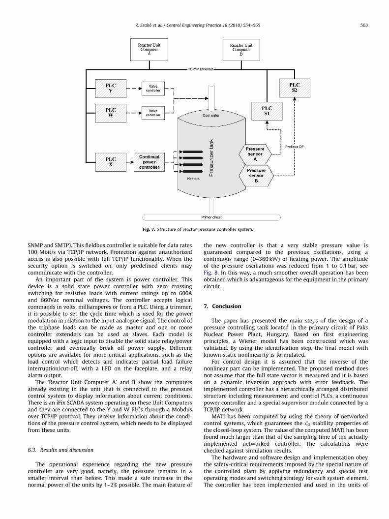
The structure of the pressure controller system is shown inFig. 7. Pressure sensors A, B and a Profibus DP pressure sensormeasure the pressure in the pressurizer. Sampling time is 250 ms,the measurements are processed by PLCs S1 and S2 using anaveraging filter. Since the physical location of the pressuremeasurement is not identical to the place to which the controlledpressure corresponds, the pressure difference resulting from theheight difference should be taken into account (also in PLCs S1and S2). In each sampling instant, both sensors send a pressuremeasurement through the Profibus DP network, but only oneselected record will be processed. The selection primarily dependson the first correct measurement record and on the credibility ofcertain signals. The selection procedure runs in PLCs Y, X and Wsuch that all three PLCs must select the same pressure value. Thisrequires that the selection procedures to be implemented usingmajority (2v3) voting logic that must be free of any functionalhazards. The main tasks of PLCs S1 and S2 are the pre-processingand transmission of pressure measurements towards PLC units Y,X and W. The other task of these units is the organization ofcommunication between other units. The two PLCs control thetransmission of messages in the network which means that eachpacket reaches its target through these units.

The Y, X, and W PLCs contain the control algorithm and thesedevices drive the real actuators. These fieldbus controllers arecapable of supporting all I/O modules. The Y, X, W devicesautomatically configure themselves, creating a local processimage which may include analog, digital or specialty modules.They are programmable according to IEC 61131-3 with 512 kBprogram memory, 128 kB data memory and 24 kB retentivememory. The 32-bit based CPU is capable of multitasking andhas a battery-backed real-time clock. The controller offers manydifferent application protocols which can be used for dataacquisition or control (MODBUS, ETHERNET /IP) or for systemmanaging and diagnostics (HTTP, BootP, DHCP, DNS, SNTP, FTP,

ARTICLE IN PRESS

Fig. 7. Structure of reactor pressure controller system.

Z. Szabo et al. / Control Engineering Practice 18 (2010) 554–565 563

SNMP and SMTP). This fieldbus controller is suitable for data rates100 Mbit/s via TCP/IP network. Protection against unauthorizedaccess is also possible with full TCP/IP functionality. When thesecurity option is switched on, only predefined clients maycommunicate with the controller.

An important part of the system is power controller. Thisdevice is a solid state power controller with zero crossingswitching for resistive loads with current ratings up to 600Aand 660Vac nominal voltages. The controller accepts logicalcommands in volts, milliamperes or from a PLC. Using a trimmer,it is possible to set the cycle time which is used for the powermodulation in relation to the input analogue signal. The control ofthe triphase loads can be made as master and one or morecontroller extenders can be used as slaves. Each model isequipped with a logic input to disable the solid state relay/powercontroller and eventually break off power supply. Differentoptions are available for more critical applications, such as theload control which detects and indicates partial load failureinterruption/cut-off, with a LED on the faceplate, and a relayalarm output.

The ‘Reactor Unit Computer A’ and B show the computersalready existing in the unit that is connected to the pressurecontrol system to display information about current conditions.There is an iFix SCADA system operating on these Unit Computersand they are connected to the Y and W PLCs through a Mobdusover TCP/IP protocol. They receive information about the condi-tions of the pressure control system, which needs to be displayedfrom these units.

6.3. Results and discussion

The operational experience regarding the new pressurecontroller are very good, namely, the pressure remains in asmaller interval than before. This made a safe increase in thenormal power of the units by 1–2% possible. The main feature of

the new controller is that a very stable pressure value isguaranteed compared to the previous oscillations, using acontinuous range (0–360 kW) of heating power. The amplitudeof the pressure oscillations was reduced from 1 to 0.1 bar, seeFig. 8. In this way, a much smoother overall operation has beenobtained which is advantageous for the equipment in the primarycircuit.

7. Conclusion

The paper has presented the main steps of the design of apressure controlling tank located in the primary circuit of PaksNuclear Power Plant, Hungary. Based on first engineeringprinciples, a Wiener model has been constructed which wasvalidated. By using the identification step, the final model withknown static nonlinearity is formulated.

For control design it is assumed that the inverse of thenonlinear part can be implemented. The proposed method doesnot assume that the full state vector is measured and it is basedon a dynamic inversion approach with error feedback. Theimplemented controller has a hierarchically arranged distributedstructure including measurement and control PLCs, a continuouspower controller and a special supervisor module connected by aTCP/IP network.

MATI has been computed by using the theory of networkedcontrol systems, which guarantees the L2 stability properties ofthe closed-loop system. The value of the computed MATI has beenfound much larger than that of the sampling time of the actuallyimplemented networked controller. The calculations werechecked against simulation results.

The hardware and software design and implementation obeythe safety-critical requirements imposed by the special nature ofthe controlled plant by applying redundancy and special testoperating modes and switching strategy for each system element.The controller has been implemented and used in the units of

ARTICLE IN PRESS

55 60 65 70122.2

122.4

122.6

122.8

123

123.2

123.4

123.6

123.8

time [h]

prim

ary

circ

uit p

ress

ure

[bar

]

new controllerold controller

Fig. 8. Pressure before and after the implementation of the new control scheme.

Z. Szabo et al. / Control Engineering Practice 18 (2010) 554–565564

Paks NPP. The use of the advanced controller resulted in a smoothoverall operation, which is advantageous for the equipment in theprimary circuit. In addition, it has been possible to safely increasethe thermal power of the units by 1–2%.

Acknowledgments

The work was supported by the Control Engineering ResearchGroup of HAS at Budapest University of Technology andEconomics. The support of the Hungarian Scientific ResearchFund through Grants T042710, F046223 is gratefully acknowl-edged. Gabor Szederkenyi is the grantee of Bolyai Janos ResearchScholarship of the Hungarian Academy of Sciences.

The authors gratefully acknowledge the continuous support ofthe members of the INC Refurbishment Project, especially thehelp of Tamas Turi, Bela Katics and Balazs Doszpod at PaksNuclear Power Plant.

The authors also thank the anonymous reviewers for theirsuggestions and comments.

References

APROS, 2005. APROS—The advanced process simulation environment. VTTIndustrial Systems. /http://www.apros.fi/en/S.

Astrom, K. J., & Bell, R. D. (2000). Drum-boiler dynamics. Automatica, 36, 363–378.Basile, G., & Marro, G. (1973). A new characterization of some structural properties

of linear systems: unknown-input observability, invertibility and functionalcontrollability. International Journal on Control, 17, 931–943.

Bloemen, H., van den Boom, T. J. J., & Verbruggen, H. (2001). Model-based predictivecontrol for Hammerstein–Wiener systems. International Journal of Control, 74,482–495.

Bokor, J., Keviczky, L. (1985). Recursive structure, parameter and delay timeestimation using ESS representations. In 7th IFAC symposium on identificationand system parameter estimation (pp. 867–872), York (UK).

di Benedetto, M. D., & Grizzle, J. (1991). Asymptotic model matching for nonlinearsystems. IEEE Transactions on Automatic Control, 39, 1539–1550.

Fazekas, C., Szederkenyi, G., & Hangos, K. M. (2008). Parameter estimation of asimple primary circuit model of a VVER plant. IEEE Transactions on NuclearScience, 55, 2643–2653.

Fazekas, C., Szederkenyi, G., & Hangos, K. M. (2009). A simple dynamic model of theprimary circuit in VVER plants for controller design purposes. NuclearEngineering and Design, 237, 1071–1087.

Grewal, M., & Glover, K. (1976). Identifiability of linear and nonlinear dynamicalsystems. IEEE Transactions on Automatic Control, 21, 833–837.

Hangos, K., & Cameron, I. (2001). Process modelling and model analysis. London:Academic Press.

Hirschorn, R. (1981). Output tracking in multivariable nonlinear systems. IEEETransactions on Automatic Control, 26, 593–595.

Huang, J., & Rugh, W. (1990). On nonlinear multivariable servomechanismproblem. Automatica, 26, 963–972.

Isidori, A. (1985). The matching of a prescribed linear input–output behaviour in anonlinear system. IEEE Transactions on Automatic Control, 30, 258–265.

Jin, J., Ko, S., & Ryoo, C.-K. (2008). Fault tolerant control for satellites with fourreaction wheels. Control Engineering Practice, 16, 1250–1258.

Kalafatis, A. D., Wang, L., & Cluett, W. (1997). Identification of Wiener-typenonlinear systems in a noisy environment. International Journal on Control, 66,923–941.

Karve, A. A., Uddin, R., & Dorning, J. J. (1997). Stability analysis of BWR nuclear-coupled thermal-hydraulics using a simple model. Nuclear Engineering andDesign, 177, 155–177.

Keviczky, L., Bokor, J., & Banyasz, C. (1979). A new identification method withspecial parametrization for model structure determination. In 5th IFACsymposium on identification and system parameter estimation (pp. 561–568),Darmstadt.

Ljung, L., & Glad, T. (1994). On global identifiability of arbitrary modelparametrizations. Automatica, 30, 265–276.

Menon, P. P., Postlethwaite, I., Bennani, S., Marcos, A., & Bates, D. G. (2009).Robustness analysis of a reusable launch vehicle flight control law. ControlEngineering Practice, 17, 751–765.

Nesic, D., & Teel, A. (2004). Input-output stability properties of networked controlsystems. IEEE Transactions on Automatic Control, 49, 1650–1667.

Perry, R. H., & Green, D. W. (1999). Perry’s chemical engineers’ handbook (7th ed.).New York: McGraw-Hill.

Szabo, Z., Gaspar, P., & Bokor, J. (2005). Reference tracking of Wiener systems usingdynamic inversion. In Prep. 2005 international symposium on intelligent control(pp. 1190–1194), Limassol, Cyprus.

Szederkenyi, G. (2009). Identifiability study of a pressurizer in a pressurizedwater nuclear power plant. In European control conference—ECC 2009 (pp.3503–3508), Budapest, Hungary.

Szederkenyi, G., Szabo, Z., Bokor, J., & Hangos, K. (2008). Analysis of the networkedimplementation of the primary circuit pressurizer controller at a nuclearpower plant. In 16th Mediterranean conference on control and automation,MED’08, (pp. 1604–1609), Ajaccio, Corsica, France.

Tabbara, M., Nesic, D., & Teel, A. (2007). Stability of wireless and wireline networkedcontrol systems. IEEE Transactions on Automatic Control, 52, 1615–1630.

Tunali, E. T., & Tarn, T. J. (1987). New results for identifiability of nonlinearsystems. IEEE Transactions on Automatic Control, 32, 146–154.

ARTICLE IN PRESS

Z. Szabo et al. / Control Engineering Practice 18 (2010) 554–565 565

Varga, I., Szederkenyi, G., Hangos, K., Bokor, J. (2006). Modeling and modelidentification of a pressurizer at the Paks Nuclear Power Plant. In 14th IFACsymposium on system identification—SYSID 2006 (pp. 678–683), Newcastle,Australia.

Vatanski, N., Georges, J.-P., Auburn, C., Rondeau, E., & Jamsa-Jounela, S.-L. (2009).Networked control with delay measurement and estimation. Control Engineer-ing Practice, 17, 231–244.

Voros, J. (1995). Identification of nonlinear dynamic systems using extendedHammerstein and Wiener models. Control-Theory and Advanced Technology, 10,1203–1212.

Wellers, M., & Kositza, N. (1999). Stable nonlinear model predictive controlof constrained Wiener and Hammerstein models. In ISA-TECH Interkama 99(pp. 333–341). Germany: Dusseldorf.

Westwick, D., & Verhaegen, M. (1996). Identifying MIMO Wiener systemsusing subspace model identification methods. Signal Processing, 52,235–258.

Wonham, W. M. (1985). Linear multivariable control—A geometric approach. Berlin:Springer.

Workshop Material (2003). Pressurized water reactor simulator. InternationalAtomic Energy Agency, Vienna. IAEA-TCS-22.