Identiflcation of Some Nonlinear Systems by Using Least ... · Identiflcation of Some Nonlinear...
131
Identification of Some Nonlinear Systems by Using Least-Squares Support Vector Machines a thesis submitted to the department of electrical and electronics engineering and the institute of engineering and sciences of bilkent university in partial fulfillment of the requirements for the degree of master of science By Mahmut Yavuzer August 2010
Transcript of Identiflcation of Some Nonlinear Systems by Using Least ... · Identiflcation of Some Nonlinear...
Identification of Some Nonlinear Systems by Using Least-Squares
Support Vector Machines
a thesis
submitted to the department of electrical and electronics
engineering
and the institute of engineering and sciences
of bilkent university
in partial fulfillment of the requirements
for the degree of
master of science
By
Mahmut Yavuzer
August 2010

I certify that I have read this thesis and that in my opinion it is fully adequate,
in scope and in quality, as a thesis for the degree of Master of Science.
Prof. Dr. Omer Morgul(Supervisor)
I certify that I have read this thesis and that in my opinion it is fully adequate,
in scope and in quality, as a thesis for the degree of Master of Science.
Prof. Dr. A. Enis Cetin
I certify that I have read this thesis and that in my opinion it is fully adequate,
in scope and in quality, as a thesis for the degree of Master of Science.
Assist. Prof. Selim Aksoy
Approved for the Institute of Engineering and Sciences:
Prof. Dr. Levent OnuralDirector of Institute of Engineering and Sciences
ii
ABSTRACT
Identification of Some Nonlinear Systems by Using Least-Squares
Support Vector Machines
Mahmut Yavuzer
M.S. in Electrical and Electronics Engineering
Supervisor: Prof. Dr. Omer Morgul
August 2010
The well-known Wiener and Hammerstein type nonlinear systems and their various com-
binations are frequently used both in the modeling and the control of various electrical,
physical, biological, chemical, etc... systems. In this thesis we will concentrate on the
parametric identification and control of these type of systems. In literature, various iden-
tification methods are proposed for the identification of Hammerstein and Wiener type
of systems. Recently, Least Squares-Support Vector Machines (LS-SVM) are also applied
in the identification of Hammerstein type systems. In the majority of these works, the
nonlinear part of Hammerstein system is assumed to be algebraic, i.e. memoryless. In
this thesis, by using LS-SVM we propose a method to identify Hammerstein systems
where the nonlinear part has a finite memory. For the identification of Wiener type sys-
tems, although various methods are also available in the literature, one approach which is
proposed in some works would be to use a method for the identification of Hammerstein
type systems by changing the roles of input and output. Through some simulations it
was observed that this approach may yield poor estimation results. Instead, by using
LS-SVM we proposed a novel methodology for the identification of Wiener type sys-
tems. We also proposed various modifications of this methodology and utilized it for
some control problems associated with Wiener type systems. We also proposed a novel
iii
methodology for identification of NARX (Nonlinear Auto-Regressive with eXogenous in-
puts) systems. We utilize LS-SVM in our methodology and we presented some results
which indicate that our methodology may yield better results as compared to the Neural
Network approximators and the usual Support Vector Regression (SVR) formulations.
We also extended our methodology to the identification of Wiener-Hammerstein type
systems. In many applications the orders of the filter, which represents the linear part of
the Wiener and Hammerstein systems, are assumed to be known. Based on LS-SVR, we
proposed a methodology to estimate true orders.
Keywords: System Identification, Wiener Systems, Hammerstein Systems, Wiener-Hammerstein
Systems, Nonlinear Auto-Regressive with eXogenous inputs (NARX), Least-Squares Sup-
port Vector Machines (LS-SVM), Least-Squares Support Vector Regression (LS-SVR),
Control.
iv
OZET
DOGRUSAL OLMAYAN BAZI SISTEMLERIN EN KUC. UK KARELI
DESTEK VEKTOR MAKINELERIYLE TANILANMASI
Mahmut Yavuzer
Elektrik ve Elektronik Muhendisligi Bolumu Yuksek Lisans
Tez Yoneticisi: Prof. Dr. Omer Morgul
Agustos 2010
Bilindik Wiener ve Hammerstein turu dogrusal olmayan sistemler ve onların degisik kom-
binasyonları, cesitli elektriksel, fiziksel, biyolojik, kimyasal v.b. sistemlerin modellen-
mesinde sıklıkla kullanılmaktadır. Bu tezde, bu tur sistemlerin parametrik tanılanması
ve kontrolu uzerine yogunlasacagız. Konuyla ilgili olarak, Hammerstein ve Wiener turu
sistemlerin tanılanmasıyla ilgili olarak cesitli metotlar onerilmektedir. Son calısmalarda,
En Kucuk Kareli - Destek Vektor Makineleri (EK-DVM) de Hammerstein turu sis-
temlerin tanılanmasında kullanılmıstır. Bu calısmaların buyuk kısmında, Hammerstein
sisteminin dogrusal olmayan bolumunun cebirsel, yani belleksiz oldugu varsılmaktadır.
Bu tezde EK-DVM kullanarak, Hammerstein sistemlerini tanılayacak, dogrusal olmayan
bolumun kısıtlı bir bellege sahip oldugu bir metot oneriyoruz. Wiener turu sistemlerin
tanılanması icin literaturde pek cok metot mevcut olsa da, bazı calısmalarda one surulmus
bir yaklasım, girdi ve cıktıların rolleri degistirilerek Hammerstein sistemi icin kullanılan
metotun uygulanması seklindedir. Bazı simulasyonlar sırasında bu yontemin zayıf tahmin
sonucları verdigi gozlemlenmistir. Bunun yerine EK-DVM kullanarak Wiener turu sis-
temlerin tanılanması icin yeni bir teknik oneriyoruz. Ayrıca bu teknigi, bazı degisiklikler
onererek, Wiener turu sistemlerle ilgili bazı kontrol problemlerinde kullandık. Ayrıca
DOBH (Dogrusal Olmayan Otomatik Baglanımlı ve Harici Girdili) sistemlerin tanılanması
icin yeni bir metot sunduk. Yaklasımımızda EK-DVM den faydalanarak, sinirsel ag
iv
yakınlastırıcılar ve Destek Vektor Baglanımı (DVB) kullanımından daha iyi sonuclar
elde ettik. Ayrıca metodumuzu Wiener-Hammerstein turu sistemlerin tanılanması icin
genislettik. Pek cok uygulamada Wiener ve Hammerstein turu sistemlerin dogrusal
kısmını temsil eden filtrelerin derecelerinin bilindigi varsayılmaktadır. EK-DVB ye daya-
narak, dogru dereceyi tahmin edecek bir metot onerdik.
Anahtar Kelimeler: Sistem Tanılama, Wiener Sistemleri, Hammerstein Sistemleri, Wiener-
Hammerstein Sistemleri, Dogrusal Olmayan Otomatik Baglanımlı ve Harici girdili (DOBH)
Sistemler, En Kucuk Kareli-Destek Vektor Makineleri (EK-DVM), En Kucuk Kareli-
Destek Vektor Baglanımı (EK-DVB), Kontrol
v

ACKNOWLEDGMENTS
I would like to express my deep gratitude to my supervisor Prof. Dr. Omer Morgul
for his guidance and support throughout my study. This work is an achievement of his
invaluable advice and guidance.
I would like to thank Prof. Dr. A. Enis Cetin and Assist. Prof. Selim Aksoy for
reading and commenting on this thesis and for being my thesis committee.
I would like to thank Bilkent University EE Department and TUBITAK for their
financial support.
I also extend my thanks to my friends from my department, Suat Bayram, Aykut
Yıldız, Derya Gol, A. Kadir Eryıldırım and Bahaeddin Eravcı for their invaluable discus-
sions on science, technology, politics and sports.
Additionally, there are a number of people from my office who helped me along the
way. I am very thankful to Ismail Uyanık, Naci Saldı, A. Nail Inal and Veli Tayfun Kılıc
for our wonderful late night studies and discussions.
Finally, but forever I would like to thank my parents, Hasan and Emine Yavuzer for
their love, support and encouragement.
vii

viii
Contents
1 INTRODUCTION 1
2 SYSTEM IDENTIFICATION AND PRELIMINARIES 6
2.1 System Identification . . . . . . . . . . . . . . . . . . . . . . . . . . . . . 6
2.1.1 Types of Models . . . . . . . . . . . . . . . . . . . . . . . . . . . 8
2.1.2 Typical System Identification Procedure . . . . . . . . . . . . . . 9
2.2 Support Vector Machines For Various Tasks . . . . . . . . . . . . . . . . 9
3 A NEW FORMULATION FOR SUPPORT VECTOR REGRESSION
AND ITS USAGE FOR BILINEAR SYSTEM IDENTIFICATION 14
3.1 Nonlinear System Regression . . . . . . . . . . . . . . . . . . . . . . . . 15
3.2 LS-SVM Regression . . . . . . . . . . . . . . . . . . . . . . . . . . . . . 16
3.3 Feedforward Neural Network Regression . . . . . . . . . . . . . . . . . . 22
3.3.1 Feedforward Network . . . . . . . . . . . . . . . . . . . . . . . . . 23
3.4 Improved performance using multiple kernels . . . . . . . . . . . . . . . . 26
3.5 Determining the orders of an ARMA(p,q) by LS-SVR . . . . . . . . . . . 30
4 IDENTIFICATION AND CONTROL OF WIENER SYSTEMS BY LS-
SVM 35
4.1 Hammerstein Model Identification Using LS-SVM . . . . . . . . . . . . . 35
4.1.1 An illustrative example . . . . . . . . . . . . . . . . . . . . . . . . 39
4.2 Identification of Hammerstein Model in Case of Nonlinearity with Memory 40
4.2.1 Example . . . . . . . . . . . . . . . . . . . . . . . . . . . . . . . . 43
viii
4.3 Proposed Wiener Identification and Results . . . . . . . . . . . . . . . . 45
4.3.1 Example . . . . . . . . . . . . . . . . . . . . . . . . . . . . . . . . 47
4.4 Wiener Model Identification Using Small Signal Analysis . . . . . . . . . 50
4.4.1 Example . . . . . . . . . . . . . . . . . . . . . . . . . . . . . . . . 54
4.5 Another Approach for Wiener Model Identification . . . . . . . . . . . . 56
4.5.1 Determination of the magnitude of the input signal . . . . . . . . 56
4.5.2 Identification of Wiener Model . . . . . . . . . . . . . . . . . . . . 57
4.5.3 Example . . . . . . . . . . . . . . . . . . . . . . . . . . . . . . . . 60
4.6 Identification for any nonlinear function . . . . . . . . . . . . . . . . . . 62
4.6.1 Example . . . . . . . . . . . . . . . . . . . . . . . . . . . . . . . . 63
4.6.2 Example . . . . . . . . . . . . . . . . . . . . . . . . . . . . . . . . 65
4.7 Control of Wiener Systems After Identification . . . . . . . . . . . . . . . 66
4.7.1 Example . . . . . . . . . . . . . . . . . . . . . . . . . . . . . . . . 68
5 IDENTIFICATION OFWIENER-HAMMERSTEIN SYSTEMS BY LS-
SVM 73
5.1 Identification For Known Nonlinearity . . . . . . . . . . . . . . . . . . . 74
5.1.1 Example . . . . . . . . . . . . . . . . . . . . . . . . . . . . . . . . 79
5.2 Identification For Unknown Nonlinearity . . . . . . . . . . . . . . . . . . 82
5.2.1 Example . . . . . . . . . . . . . . . . . . . . . . . . . . . . . . . . 85
5.3 Black Box Identification of Wiener-Hammerstein Models . . . . . . . . . 85
6 CONCLUSIONS 87
APPENDIX 90
A The Matlab Codes 90
A.1 NARX System Identification Simulation Codes . . . . . . . . . . . . . . . 90
A.2 Wiener System Identification Simulation Codes . . . . . . . . . . . . . . 98
A.3 Wiener-Hammerstein System Identification Simulation Codes . . . . . . . 105
ix

List of Figures
1.1 Block diagram of a Hammerstein model . . . . . . . . . . . . . . . . . . . 2
1.2 Block diagram of a Wiener model . . . . . . . . . . . . . . . . . . . . . . 2
2.1 A dynamic system with input ut output yt and disturbance vt . . . . . . 7
2.2 Torque applied to ankles which is stimulated by neuron cells’ inputs . . 8
2.3 A flowchart for system identification . . . . . . . . . . . . . . . . . . . . 10
2.4 Optimal hyperplane is the plane that divides convex hulls of both classes. 12
3.1 The actual output values vs the estimated output values. . . . . . . . . . 21
3.2 The neuron model used in the feedforward network.©MATLAB . . . . . 23
3.3 A possible transfer function used to activate neurons.©MATLAB . . . . 23
3.4 A Feedforward neural network.©MATLAB . . . . . . . . . . . . . . . . 24
3.5 The actual output values vs the estimated output values using Neural
Networks. . . . . . . . . . . . . . . . . . . . . . . . . . . . . . . . . . . . 25
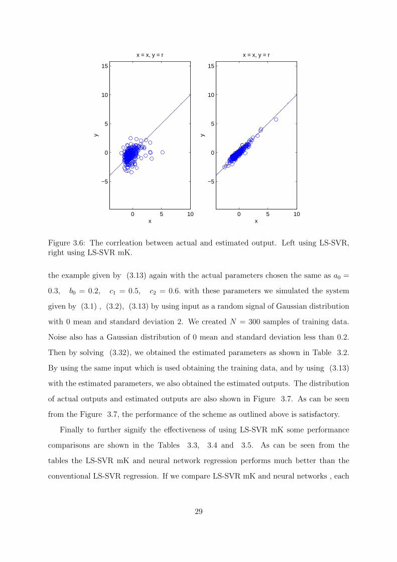
3.6 The corrleation between actual and estimated output. Left using LS-SVR,
right using LS-SVR mK. . . . . . . . . . . . . . . . . . . . . . . . . . . . 29
3.7 The actual output values vs the estimated output values using LS-SVR mK. 30
3.8 The normalized error between actual and estimated outputs as the lags
increases. . . . . . . . . . . . . . . . . . . . . . . . . . . . . . . . . . . . 33
3.9 The normalized error between actual and estimated outputs as the lags
increases for numerator order. . . . . . . . . . . . . . . . . . . . . . . . . 34
4.1 Block diagram of a Hammerstein model . . . . . . . . . . . . . . . . . . . 36
4.2 Actual and estimated outputs . . . . . . . . . . . . . . . . . . . . . . . . 41
x

4.3 Hammerstein model where the nonlinearity has memory . . . . . . . . . 41
4.4 The actual and estimated nonlinear function. RMSE = 0.8402 . . . . . . 44
4.5 Block diagram of a Wiener model . . . . . . . . . . . . . . . . . . . . . . 45
4.6 Block diagram of a Wiener model the case that the nonlinear function is
identity . . . . . . . . . . . . . . . . . . . . . . . . . . . . . . . . . . . . 50
4.7 A non-invertible nonlinear function of various break points and slopes . 51
4.8 The equivalent model when small signal is used . . . . . . . . . . . . . . 52
4.9 The designed system to obtain all the nonlinear function and breakaway
points . . . . . . . . . . . . . . . . . . . . . . . . . . . . . . . . . . . . . 52
4.10 Equivalent modified system . . . . . . . . . . . . . . . . . . . . . . . . . 53
4.11 The estimated nonlinear function in the case that there is no noise. RMSE
= 0.2822 . . . . . . . . . . . . . . . . . . . . . . . . . . . . . . . . . . . . 55
4.12 The flowchart for choosing the optimal signal to identify the system. . . . 58
4.13 The actual Wiener model is as at the top figure. We can put the gain in
front of the filter when small signals are used as in the bottom figure. . . 59
4.14 The designed system for identifying the whole of static nonlinear function. 59
4.15 The actual and estimated static nonlinear function. . . . . . . . . . . . . 61
4.16 The static nonlinear function sinc(u)u2, and the margins where it can be
approximated by some linear gains. . . . . . . . . . . . . . . . . . . . . . 62
4.17 Signals on various points of the Wiener system. Upper plot: input to the
system, middle plot : output of the linearity which is also input to the
nonlinearity, bottom plot: output of the whole system. . . . . . . . . . . 64
4.18 The histogram of the input and output data. As it is seen both seem to
have gaussian distribution of different mean and standard deviation . . . 65
4.19 Non-invertible sin(x)x is modeled with an accurate precision. RMSE =
0.1682 . . . . . . . . . . . . . . . . . . . . . . . . . . . . . . . . . . . . . 66
4.20 The designed closed loop Wiener system for control. . . . . . . . . . . . . 67
4.21 A controller is added to make the overall system stable and meet design
specifications. . . . . . . . . . . . . . . . . . . . . . . . . . . . . . . . . . 67
xi
4.22 The step response of the closed loop system is unstable. . . . . . . . . . . 68
4.23 After the controller is added the system became stable. . . . . . . . . . . 69
4.24 Actual nonlinearities and their inverses. . . . . . . . . . . . . . . . . . . . 70
4.25 Sinusoidal response of the actual filter. . . . . . . . . . . . . . . . . . . . 70
4.26 Sinusoidal response of the filter. The response is oscillatory for the chosen
integral controller gain. . . . . . . . . . . . . . . . . . . . . . . . . . . . . 71
4.27 Sinusoidal response of the filter. The controller gain is still not appropriate 71
4.28 Sinusoidal response of the filter. The oscillations have died. . . . . . . . . 72
5.1 The Wiener-Hammerstein system . . . . . . . . . . . . . . . . . . . . . . 74
5.2 The Wiener-Hammerstein system as a Hammerstein model . . . . . . . . 76
5.3 The equivalent Wiener-Hammerstein system when small signals are used. 77
5.4 The equivalent Wiener-Hammerstein system when small signals are used.
E(z) is convolution of the first and second filter. . . . . . . . . . . . . . . 79
5.5 The poles and zeroes of actual and estimated filter. . . . . . . . . . . . . 81
5.6 Step responses of actual and estimated filters at various points. As it is
seen in the bottom figure both responses are almost indistinguishable . . 81
5.7 The actual and estimated output, top plot: correct sharing, bottom: wrong
sharing. . . . . . . . . . . . . . . . . . . . . . . . . . . . . . . . . . . . . 82
5.8 The designed system to model the static nonlinearity so that the identifi-
cation be complete. . . . . . . . . . . . . . . . . . . . . . . . . . . . . . . 83
5.9 The outputs of both estimated filters are plotted against each other. The
first one is the true nonlinearity, the last one is the true estimated nonlin-
earity. . . . . . . . . . . . . . . . . . . . . . . . . . . . . . . . . . . . . . 84
xii
List of Tables
3.1 Actual and estimated linear parameters . . . . . . . . . . . . . . . . . . . 21
3.2 Actual and estimated linear parameters . . . . . . . . . . . . . . . . . . . 30
3.3 Correlation and RMSE errors by LS-SVR . . . . . . . . . . . . . . . . . . 31
3.4 Correlation and RMSE errors by LS-SVR mK . . . . . . . . . . . . . . . 31
3.5 Correlation and RMSE errors by Neural Networks . . . . . . . . . . . . . 31
4.1 Actual and identified AR parameters . . . . . . . . . . . . . . . . . . . . 40
4.2 Actual and Estimated MA parameters . . . . . . . . . . . . . . . . . . . 40
4.3 Actual and identified AR parameters . . . . . . . . . . . . . . . . . . . . 43
4.4 Actual and Estimated MA parameters . . . . . . . . . . . . . . . . . . . 44
4.5 Actual and identified AR parameters . . . . . . . . . . . . . . . . . . . . 48
4.6 Actual and Estimated MA parameters . . . . . . . . . . . . . . . . . . . 48
4.7 Ar parameters of actual and estimated Wiener Model . . . . . . . . . . . 54
4.8 MA parameters of actual and estimated Wiener Model . . . . . . . . . . 55
4.9 AR parameters of actual and estimated Wiener Model . . . . . . . . . . 60
4.10 MA parameters of actual and estimated Wiener Model . . . . . . . . . . 60
4.11 AR parameters of actual and estimated Wiener Model . . . . . . . . . . 66
4.12 MA parameters of actual and estimated Wiener Model . . . . . . . . . . 67
5.1 AR parameters of actual and estimated Wiener Model . . . . . . . . . . 80
5.2 MA parameters of actual and estimated Wiener Model . . . . . . . . . . 80
5.3 Goodness-of-fit (gof) and normalized mean absolute error (nmae) of the
proposed model SVR model , LSL model and Hill Huxley model . . . . . 86
xiii

Dedicated to my family
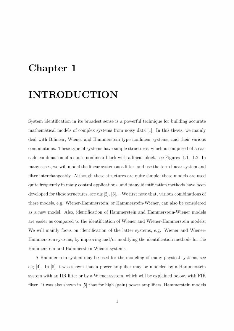
Chapter 1
INTRODUCTION
System identification in its broadest sense is a powerful technique for building accurate
mathematical models of complex systems from noisy data [1]. In this thesis, we mainly
deal with Bilinear, Wiener and Hammerstein type nonlinear systems, and their various
combinations. These type of systems have simple structures, which is composed of a cas-
cade combination of a static nonlinear block with a linear block, see Figures 1.1, 1.2. In
many cases, we will model the linear system as a filter, and use the term linear system and
filter interchangeably. Although these structures are quite simple, these models are used
quite frequently in many control applications, and many identification methods have been
developed for these structures, see e.g [2], [3], . We first note that, various combinations of
these models, e.g. Wiener-Hammerstein, or Hammerstein-Wiener, can also be considered
as a new model. Also, identification of Hammerstein and Hammerstein-Wiener models
are easier as compared to the identification of Wiener and Wiener-Hammerstein models.
We will mainly focus on identification of the latter systems, e.g. Wiener and Wiener-
Hammerstein systems, by improving and/or modifying the identification methods for the
Hammerstein and Hammerstein-Wiener systems.
A Hammerstein system may be used for the modeling of many physical systems, see
e.g [4]. In [5] it was shown that a power amplifier may be modeled by a Hammerstein
system with an IIR filter or by a Wiener system, which will be explained below, with FIR
filter. It was also shown in [5] that for high (gain) power amplifiers, Hammerstein models
1
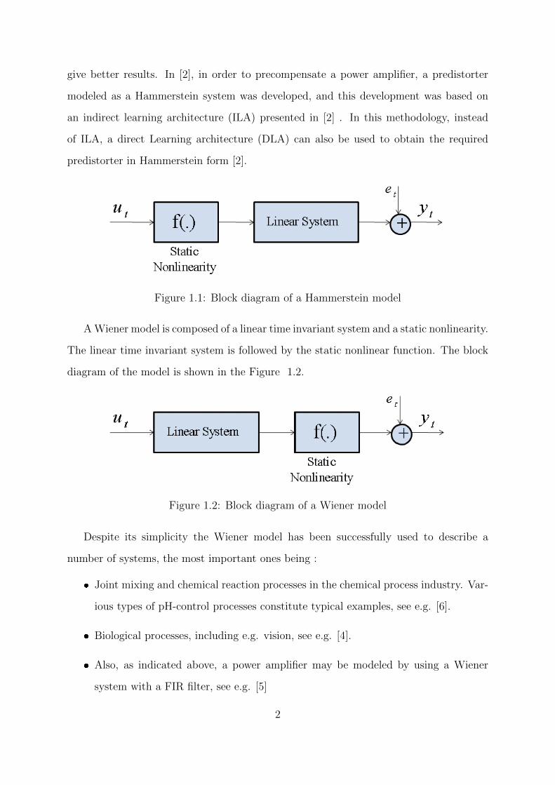
give better results. In [2], in order to precompensate a power amplifier, a predistorter
modeled as a Hammerstein system was developed, and this development was based on
an indirect learning architecture (ILA) presented in [2] . In this methodology, instead
of ILA, a direct Learning architecture (DLA) can also be used to obtain the required
predistorter in Hammerstein form [2].
Figure 1.1: Block diagram of a Hammerstein model
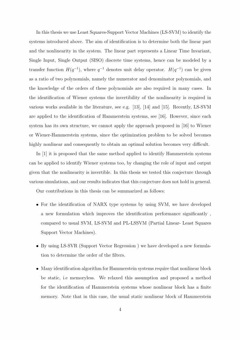
AWiener model is composed of a linear time invariant system and a static nonlinearity.
The linear time invariant system is followed by the static nonlinear function. The block
diagram of the model is shown in the Figure 1.2.
Figure 1.2: Block diagram of a Wiener model
Despite its simplicity the Wiener model has been successfully used to describe a
number of systems, the most important ones being :
Joint mixing and chemical reaction processes in the chemical process industry. Var-
ious types of pH-control processes constitute typical examples, see e.g. [6].
Biological processes, including e.g. vision, see e.g. [4].
Also, as indicated above, a power amplifier may be modeled by using a Wiener
system with a FIR filter, see e.g. [5]
2

What is less well known is that the Wiener model is also useful for the description of a
number of situations where the measurement of the output of a linear system is highly
nonlinear and non-invertible. Important examples include
Saturation in the output measurements, see e.g. [7].
Dead zones in the output measurements, see e.g. [7].
Output measurements which insensitive to sign, e.g. pulse counting angular rate
sensors, see e.g [3].
Quantization in the output measurements. This case has received a considerable
interest recently with the emerging techniques for network control systems, see e.g.
[8] .
Blind adaptation. This follows since the blind adaptation problem can sometimes
be cast into the form of a Wiener system, see e.g. [9]
Wiener models have also been successfully used for extremum control. A main moti-
vation for the use of Wiener models is that the dynamics is linear, a fact that simplifies
the handling of properties like statistical stationarity and stability, as compared to when
a general nonlinear model is applied.
We will also deal with NARX (Nonlinear Auto-Regressive with eXogenous inputs)
systems. These type of systems are also applied successfully to model many physical,
biological and other phenomenons. For example, in mechanical models for vibration
analysis specific polynomial nonlinearities are often used to describe well-known nonlinear
elastic or viscous behaviours, see e.g [10]. The well-known Bilinear systems can also be
considered as a subset of NARX models. Many objects in engineering, economics, ecology
and biology etc. can be described by using a bilinear system, see e.g [11]. The bilinear
systems are the simplest nonlinear systems which are similar to a linear system in its
form, [12]. In literature, mainly least-squares (LS) techniques and/or black box modeling
are used for the identification of NARX, and in particular bilinear systems.
3
In this thesis we use Least Squares-Support Vector Machines (LS-SVM) to identify the
systems introduced above. The aim of identification is to determine both the linear part
and the nonlinearity in the system. The linear part represents a Linear Time Invariant,
Single Input, Single Output (SISO) discrete time systems, hence can be modeled by a
transfer function H(q−1), where q−1 denotes unit delay operator. H(q−1) can be given
as a ratio of two polynomials, namely the numerator and denominator polynomials, and
the knowledge of the orders of these polynomials are also required in many cases. In
the identification of Wiener systems the invertibility of the nonlinearity is required in
various works available in the literature, see e.g. [13], [14] and [15]. Recently, LS-SVM
are applied to the identification of Hammerstein systems, see [16]. However, since each
system has its own structure, we cannot apply the approach proposed in [16] to Wiener
or Wiener-Hammerstein systems, since the optimization problem to be solved becomes
highly nonlinear and consequently to obtain an optimal solution becomes very difficult.
In [1] it is proposed that the same method applied to identify Hammerstein systems
can be applied to identify Wiener systems too, by changing the role of input and output
given that the nonlinearity is invertible. In this thesis we tested this conjecture through
various simulations, and our results indicates that this conjecture does not hold in general.
Our contributions in this thesis can be summarized as follows:
For the identification of NARX type systems by using SVM, we have developed
a new formulation which improves the identification performance significantly ,
compared to usual SVM, LS-SVM and PL-LSSVM (Partial Linear- Least Squares
Support Vector Machines).
By using LS-SVR (Support Vector Regression ) we have developed a new formula-
tion to determine the order of the filters.
Many identification algorithm for Hammerstein systems require that nonlinear block
be static, i.e memoryless. We relaxed this assumption and proposed a method
for the identification of Hammerstein systems whose nonlinear block has a finite
memory. Note that in this case, the usual static nonlinear block of Hammerstein
4
model is replaced by a non-static nonlinear block.
We have developed new formulations for the identification of Wiener systems, which
does not require the nonlinear block to be invertible. Note that many identification
schemes proposed in the literature for Wiener systems assume that the nonlinear
block be invertible.
We designed feedback control schemes for the control of Wiener systems by using
SVM.
In [16] Hammerstein systems are identified by using LS-SVM, and the identification
of Wiener-Hammerstein systems by using LS-SVM is set as a future problem. We
developed a methodology for the identification of Wiener-Hammerstein systems by
using LS-SVM.
In Chapter 2, we first give a brief description about system identification and some
procedures. Then we provide some mathematical preliminaries that are necessary for
the development of the work which will be presented in this thesis. Chapter 3 addresses
the mathematical model and the algorithm we developed for identification of NARX
systems. We first obtain the performance of the usual LS-SVM, then we compare it with
the performance of Neural Networks. Then we comment on the improvement we obtained
on the performance in the identification of NARX systems. In Chapter 4, we show how
LS-SVM are used for identification of Hammerstein systems. Then we modify, and design
that approach in various ways to identify Wiener systems and to control them. We also
compare and contrast our proposed algorithm with the existing algorithms presented in
[17] and [18] in terms of the mean squared errors between outputs. In Chapter 5 we
propose a novel methodology for the identification of Wiener-Hammerstein systems. by
using LS-SVM and compare the performance with some other existing methodologies,
see e.g. [19]. Finally we give some concluding remarks in Chapter 6.
5
Chapter 2
SYSTEM IDENTIFICATION AND
PRELIMINARIES
In this chapter, basic concepts of system identification are explained and some mathe-
matical preliminaries are given briefly. We will introduce system identification procedure.
Then the main systems we deal with in this thesis, namely Wiener and Hammerstein sys-
tems will be introduced. Their application areas will be explained briefly. Then we will
present some basic formulations for Support Vector Machine (SVM) classification and
regression.
2.1 System Identification
System identification is a general term that is used to describe mathematical tools and
algorithms that build dynamical models from measured data. A dynamical system is
considered to be as in Figure 2.1 The input signal is ut and the system may have some
disturbances vt. We are able to determine the input signal but not the disturbances.
Sometimes the input signal may also be assumed to be unknown. The output is assumed
to be obtained with some measurement errors as usual.
The need for a model to represent a physical system has various reasons. Consider
a human body muscle system. After Spinal Cord Injury (SCI), the loss of volitional
6
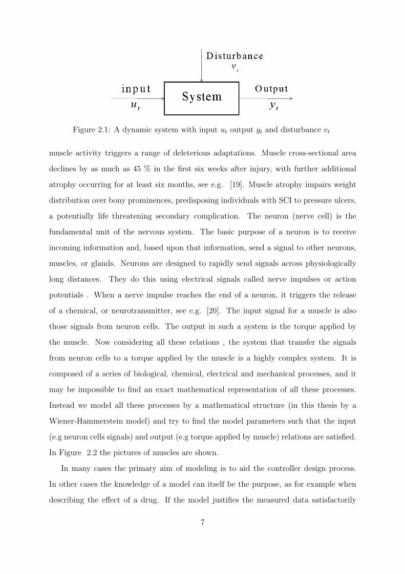
Figure 2.1: A dynamic system with input ut output yt and disturbance vt
muscle activity triggers a range of deleterious adaptations. Muscle cross-sectional area
declines by as much as 45 % in the first six weeks after injury, with further additional
atrophy occurring for at least six months, see e.g. [19]. Muscle atrophy impairs weight
distribution over bony prominences, predisposing individuals with SCI to pressure ulcers,
a potentially life threatening secondary complication. The neuron (nerve cell) is the
fundamental unit of the nervous system. The basic purpose of a neuron is to receive
incoming information and, based upon that information, send a signal to other neurons,
muscles, or glands. Neurons are designed to rapidly send signals across physiologically
long distances. They do this using electrical signals called nerve impulses or action
potentials . When a nerve impulse reaches the end of a neuron, it triggers the release
of a chemical, or neurotransmitter, see e.g. [20]. The input signal for a muscle is also
those signals from neuron cells. The output in such a system is the torque applied by
the muscle. Now considering all these relations , the system that transfer the signals
from neuron cells to a torque applied by the muscle is a highly complex system. It is
composed of a series of biological, chemical, electrical and mechanical processes, and it
may be impossible to find an exact mathematical representation of all these processes.
Instead we model all these processes by a mathematical structure (in this thesis by a
Wiener-Hammerstein model) and try to find the model parameters such that the input
(e.g neuron cells signals) and output (e.g torque applied by muscle) relations are satisfied.
In Figure 2.2 the pictures of muscles are shown.
In many cases the primary aim of modeling is to aid the controller design process.
In other cases the knowledge of a model can itself be the purpose, as for example when
describing the effect of a drug. If the model justifies the measured data satisfactorily
7
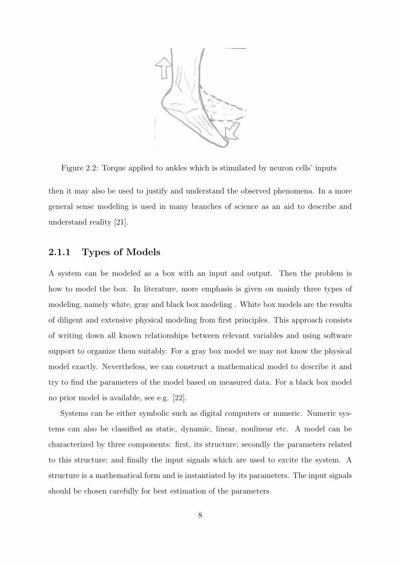
Figure 2.2: Torque applied to ankles which is stimulated by neuron cells’ inputs
then it may also be used to justify and understand the observed phenomena. In a more
general sense modeling is used in many branches of science as an aid to describe and
understand reality [21].
2.1.1 Types of Models
A system can be modeled as a box with an input and output. Then the problem is
how to model the box. In literature, more emphasis is given on mainly three types of
modeling, namely white, gray and black box modeling . White box models are the results
of diligent and extensive physical modeling from first principles. This approach consists
of writing down all known relationships between relevant variables and using software
support to organize them suitably. For a gray box model we may not know the physical
model exactly. Nevertheless, we can construct a mathematical model to describe it and
try to find the parameters of the model based on measured data. For a black box model
no prior model is available, see e.g. [22].
Systems can be either symbolic such as digital computers or numeric. Numeric sys-
tems can also be classified as static, dynamic, linear, nonlinear etc. A model can be
characterized by three components: first, its structure; secondly the parameters related
to this structure; and finally the input signals which are used to excite the system. A
structure is a mathematical form and is instantiated by its parameters. The input signals
should be chosen carefully for best estimation of the parameters.
8

2.1.2 Typical System Identification Procedure
In general terms, an identification experiment is performed by exciting the system (using
some sort of input signal such as a step, a sinusoid or a random signal -etc.) and observing
its input and output over a time interval. These signals are normally recorded in a
computer mass storage for subsequent ’information processing’. We then try to fit a
parametric model of the process to the recorded input and output sequences. The first
step is to determine an appropriate form of the model ( typically a linear difference
equation of a certain order). As a second step, some statistically based methods are used
to estimate the unknown parameters of the model (such as the coefficients in the difference
equation). In practice, the estimation of the structure and the parameters are often
done iteratively. This means that a tentative structure is chosen and the corresponding
parameters are estimated. The model obtained is then tested to determine whether it is
an appropriate representation of the system. If this is not the case, some more complex
model structures may be considered, its parameters should be estimated, the new model
should be validated, etc. The overall identification process may be given by a flowchart
as shown in Figure 2.3, which summarizes the basic steps involved in the process, see
e.g. [21].
2.2 Support Vector Machines For Various Tasks
Support vector machines (SVM) are basically used for pattern recognition and in partic-
ular for classification tasks. For simplicity, let us assume that the patterns belong to the
distinct classes, say C1 and C2. Furthermore let us assign class membership value as +1 if
a pattern belongs to C1 and −1 if a pattern belongs to C2. More precisely, let us assume
that the patterns are represented by L dimensional vectors, i.e xi ∈ RL for pattern xi,
and let us associate an output value yi for xi such that if xi ∈ C1, we have yi = +1,
and if xi ∈ C2 we have yi = −1. Furthermore let us assume that we have N training
samples, each are represented by a pair xi, yi, i = 1, . . . , N . For pattern recognition
(classification), we try to estimate a function f : RL → ±1 using training data, that is
9
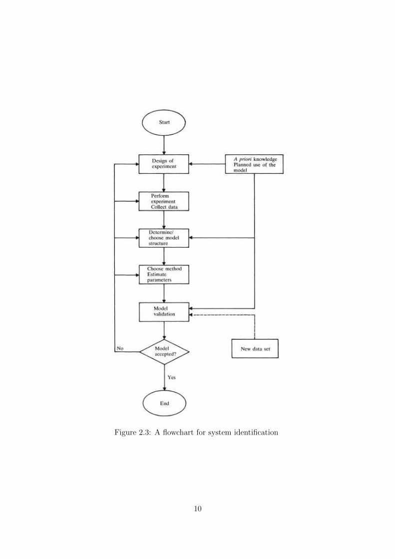
Figure 2.3: A flowchart for system identification
10
L dimensional patterns xi and class labels yi
x1, y1, . . . , xN , yN ∈ RL × ±1, (2.1)
such that f will correctly classify new examples (x, y). That is, f(x) = y for examples
(x, y) which are generated from the same underlying probability distribution P (x, y) as
the training data. If we put no restriction on the class of functions that we choose our
estimate f from, even a function that does well on the training data for example by
satisfying f(xi) = yi need not generalize well to unseen examples. Suppose that we do
not have additional information on f (for example, about its smoothness). Then the
values on the training patterns carry no information whatsoever about values on novel
patterns. Hence learning is impossible, and minimizing the training error does not imply
a small expected test error. Statistical learning theory, or VC (Vapnik-Chervonenkis)
theory, shows that it is crucial to restrict the class of functions that the learning machine
can implement to one with a capacity that is suitable for the amount of available training
data. For more information, please refer to [23].
Hyperplane classifiers
Given the training set, xi, yi, i = 1, . . . , N , and a parameterized form of the func-
tion f(.) : RL → ±1, finding the parameters of f(.) is of crucial importance for the
classification problem as stated above. There are various ways for the solution of this
problem, see e.g. [24]. and utilizing learning algorithms which basically give us an up-
date rule/algorithm to find these coefficients, is a frequently used method. To design
learning algorithms, we thus must come up with a class of functions whose capacity can
be computed. SV classifiers are based on the class of hyperplanes as given below:
< w,ϕ(x) > +d = 0 w ∈ RL, d ∈ R, (2.2)
where w ∈ RL and d ∈ R are unknown parameters to be found, < ., . > represents the
standard inner product in RL, xi ∈ RL is the pattern vector and ϕ(.) : RL → RH is
called as the ”Kernel function” , [25]. Then the corresponding decision function can be
11

given as:
f(x) = sign(< w,ϕ(x) > +d), (2.3)
where sign(.) is the standard signum function, i.e
sign(t) =
+1, if t ≥ 0,
−1, if t < 0
(2.4)
We note that the hyperplane given by ( 2.2) separates the pattern space into two half
spaces, if this hyperplane separates C1 and C2, then the signum function achieves correct
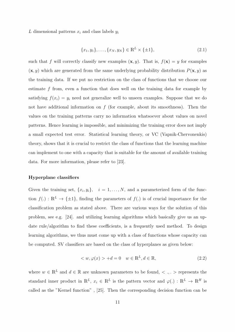
classification. One can show that the optimal hyperplane, defined as the one with the
maximal margin of separation between the two classes (see Figure 2.4), has the lowest
capacity [23]. It can be uniquely constructed by solving a constrained quadratic opti-
Figure 2.4: Optimal hyperplane is the plane that divides convex hulls of both classes.
mization problem whose solution w has an expansion w =∑N
i=1 αixi in terms of a subset
of training patterns that lie on the margin (see Figure 2.4). These training patterns,
called support vectors, carry all relevant information about the classification problem.
Because we are using kernels, we will thus obtain a nonlinear decision function of the
following form, see e.g. [25].
f(x) = sign(N∑i=1
αiK(x,xi) + d). (2.5)
12

Here xi’s represent the support vectors, and K(., .) : RH × RH → R is an appropriate
kernel function. In literature, various kernel functions such as Gaussian, Polynomial, etc.
are successfully used [26]. In our work we will mainly utilize Gaussian kernel functions,
which are given asK(xi, xj) = e(−‖xi−xj‖2) The parameters αi are computed as the solution
of a quadratic programming problem.
The most important restriction up to now has been that we consider only the classifi-
cation problem. However, a generalization to regression estimation,that is, to y ∈ R, canalso be given, see e.g. [27]. In this case, the algorithm tries to construct a linear function
in the feature space such that the training points lie within a distance ε > 0. Similar to
the pattern-recognition case, we can write this as a quadratic programming problem in
terms of kernels. The nonlinear regression estimate takes the form
f(x) =N∑i=1
αiK(x,xi) + d (2.6)
To apply the algorithm, we either specify ε a priori, or we specify an upper bound
on the fraction of training points allowed to lie outside of a distance ε from the regres-
sion estimate (asymptotically, the number of SVs) and the corresponding ε is computed
automatically. For more information refer to [26].
13
Chapter 3
A NEW FORMULATION FOR
SUPPORT VECTOR
REGRESSION AND ITS USAGE
FOR BILINEAR SYSTEM
IDENTIFICATION
In this chapter, basic concepts of Support Vector Regression (SVR) are explained. First
we will show how nonlinear functions are modeled with SVM in general. We will then
show LS-SVM regression in particular and examine its performance. Then we will present
performance of Neural Network regression. We will also present a novel methodology and
will illustrate its performance compared to usual SVM regression approach and Neural
Network approach. We will make comparisons between these three methods in terms of
their performances. Finally we will present a novel methodology to determine the order
of the filter representing the linear blocks in our model, see Figure 1.1 and 1.2
14
3.1 Nonlinear System Regression
Any nonlinear function (system) can be modeled with Support Vector Regression (SVR).
Support Vector Regression uses the same principle as the Support Vector Machine clas-
sification, with only a few minor differences. In the case of classification only two output
values are possible. But since we are trying to model a nonlinear function, the output
has infinitely many possible values, that is while in classification we have y ∈ ∓1, herewe have y ∈ R. However, the main idea is similar: to minimize the error and maximize
the margin between the optimal hyperplanes.
The nonlinear dynamical systems with an input u and an output y can be described in
discrete time by the NARX (nonlinear autoregressive with exogenous input) input output
model:
y(k) = f(x(k)), (3.1)
where f(.) is a nonlinear function, y(k) ∈ R denotes the output at the time instant
k and x(k) is the regressor vector, consisting of a finite number of past inputs and
outputs. If we assume that the current output y(k) depends on past outputs y(i) for i ∈[k − ny − 1, k − 1] and inputs u(i) for i ∈ [k − nu − 1, k], where ny and nu are appropriate
integers, then an appropriate regression vector x(k) to be used in 3.1 can be given as
follows:
x(k) =
y(k − 1)
...
y(k − ny)
u(k)
...
u(k − nu)
(3.2)
where nu is the dynamical order for the inputs and ny is the dynamical order for the
outputs, i.e. the present output depends on past ny outputs and nu inputs, as explained
above. Hence, with the above notation, we have x ∈ Rnu+ny+1, y ∈ R and f : Rnu+ny+1 →R. We note that, here the regression relation is deterministic. In a realistic situation,
output measurements are usually corrupted by some noise. For such cases, instead of
15
3.1, we may consider the following regression relation.
y(k) = f(x(k)) + ξ(k), (3.3)
where the regression vector x(.), the output y(.) and the nonlinear function f(.) are
the same as explained above; here ξ(.) represents the meausurement noise, and typically
modeled by a gaussian noise with zero mean and finite variance. Note that, for notational
simplicity we will use the notation ξi to denote ξ(i) in the sequel.
The task of system identification here is essentially to find suitable mappings, which
can approximate the mappings implied in the nonlinear dynamical system of (3.1). The
function f(.) can be approximated by some general function approximators such as neural
networks, neuro-fuzzy systems, splines, interpolated look-up tables, etc. [25]. The aim
of system identification is only to obtain an accurate predictor for y. In this work we
will show how we may increase the performance of the predictor by using appropriate
kernel mappings for each nonlinearity in the function f(.). The details will be given in
the sequel.
3.2 LS-SVM Regression
Consider a given training set of N data points xi, yi for i = 1, . . . , N , where xi ∈ Rn,
y ∈ R, (note that with the notation of (3.3), we have n = nu+ny+1). Let us assume that
the input output relation is as given by (3.1). Our aim will be based on the training data,
to find an estimation of the nonlinear function f(.). Although several techniques may
be utilized to estimate f(.), we will use SVM technique introduced in section 2. Hence,
referring to (2.6), we will try to approximate the nonlinear function f(.) as follows:
y(x) =< w,ϕ(x) > +d = wTϕ(x) + d, (3.4)
where ϕ : Rn → Rnf , where nf is left undetermined yet and usually nf ≥ n, d ∈ R. ϕ(.)is called the feature map; its role is to map the data into a higher dimensional feature
space, which could also be infinite dimensional (i.e nf = ∞) in theory. Various forms of
ϕ(.) may be used, see [28]; in this thesis we will mainly use Gaussian functions, see (3.7)
16
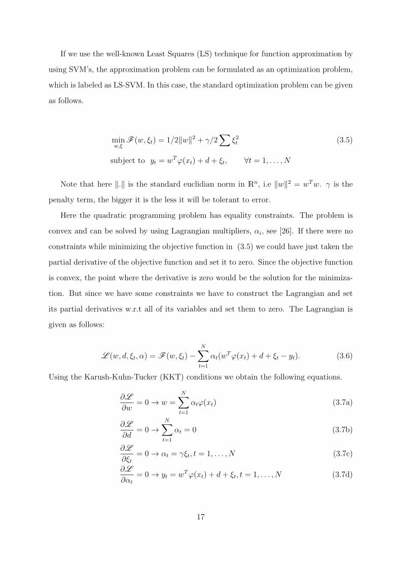
If we use the well-known Least Squares (LS) technique for function approximation by
using SVM’s, the approximation problem can be formulated as an optimization problem,
which is labeled as LS-SVM. In this case, the standard optimization problem can be given
as follows.
minw,ξ
F (w, ξt) = 1/2‖w‖2 + γ/2∑
ξ2t (3.5)
subject to yt = wTϕ(xt) + d+ ξt, ∀t = 1, . . . , N
Note that here ‖.‖ is the standard euclidian norm in Rn, i.e ‖w‖2 = wTw. γ is the
penalty term, the bigger it is the less it will be tolerant to error.
Here the quadratic programming problem has equality constraints. The problem is
convex and can be solved by using Lagrangian multipliers, αi, see [26]. If there were no
constraints while minimizing the objective function in (3.5) we could have just taken the
partial derivative of the objective function and set it to zero. Since the objective function
is convex, the point where the derivative is zero would be the solution for the minimiza-
tion. But since we have some constraints we have to construct the Lagrangian and set
its partial derivatives w.r.t all of its variables and set them to zero. The Lagrangian is
given as follows:
L (w, d, ξt, α) = F (w, ξt)−N∑t=1
αt(wTϕ(xt) + d+ ξt − yt). (3.6)
Using the Karush-Kuhn-Tucker (KKT) conditions we obtain the following equations.
∂L
∂w= 0 → w =
N∑t=1
αtϕ(xt) (3.7a)
∂L
∂d= 0 →
N∑t=1
αt = 0 (3.7b)
∂L
∂ξt= 0 → αt = γξt, t = 1, . . . , N (3.7c)
∂L
∂αt
= 0 → yt = wTϕ(xt) + d+ ξt, t = 1, . . . , N (3.7d)
17
If we put (??) and (3.7c) in (3.7d) we obtain the following:
yk =N∑t=1
αtϕ(xt)Tϕ(xk) + d+ ξk, k = 1, . . . , N (3.8)
Note that in (3.8), we have N equations. We can rewrite (3.8) and (3.7b) as a set
of linear equations in the following form:
0 1T
N
1N K+ γ−1I1TN
d
α
=
0
Y
(3.9)
Where K is a positive definite matrix and K(i, j) = ϕ(xi)Tϕ(xj) = e
(−‖xi−xj‖2)2σ2 , where
σ is a scaling factor, α = [α1α2 . . . αN ], 1TN is a vector, whose entries are 1 and d is the bias
term. The mapping ϕ(.) can be polynomial, linear etc. In 3.9 a least squares solution
is obtained in order to find α and d parameters. Since this is almost standard, we omit
the details here, interested reader may refer to [26] for details. After obtaining these
parameters, the resulting expression for estimated function will be as the following: Note
that 3.9 is a linear equation of the form Az = b, where z = [d α]T is the unknown
vector which gives the sum parameters. A LS solution to this equation can be obtained by
using various techniques see e.g.[29]. After obtaining the SVM parameters, the regressor
function f(.) can be approximated by using (3.4) as,
f(x) = wTϕ(x) + d, (3.10)
If we use (3.7a) in (3.10) we obtain
f(x) =N∑
k=1
αkϕ(x(k))Tϕ(x) + d. (3.11)
Finally if we denote the kernel K(x, xk) as K(x, xk) = ϕ(x(k))Tϕ(x), we obtain:
f(x) =N∑
k=1
αkK(x, xk) + d. (3.12)
In order to see the performance of the resulting estimated function we have done various
simulations for different systems . Assume that the system dynamics is given by (3.1),
where the nonlinear function f(x(k)) is given as:
18
f(x(k)) = (a0 + a1sin(u(k − 1)) + a2cos(u(k − 2)))y(k − 1)
+(b0 + b1sin(u(k − 1)) + b2u(k − 2))y(k − 2) + c1u(k − 1) + c2u(k − 2) (3.13)
The function f(.) given by 3.13 can be rewritten as
f(xk) = a0yk−1 + f1(uk−1, yk−1) + f2(uk−2, yk−1)
+f3(uk−1, yk−2) + f4(uk−2, yk−2). (3.14a)
f1(uk−1, yk−1) = a1sin(u(k − 1))y(k − 1) (3.14b)
f2(uk−2, yk−1) = a2cos(u(k − 2))y(k − 1) (3.14c)
f3(uk−1, yk−2) = b1sin(u(k − 1))y(k − 2) (3.14d)
f4(uk−2, yk−2) = b2u(k − 2)y(k − 2) (3.14e)
Therefore we can think of f(.) as a function that depends on xk = [uk−1 uk−2 yk−1 yk−2]T .
Hence, this function can be modeled with SVR by using xk as the regressor vector. The
leading formulations will be as the following:
minwx,ek
F (w, ξk) = 1/2wTw + γ/2N∑
k=r
ξ2k
subject to y(k) = a0y(k − 1) + b0y(k − 2) + c1u(k − 1) + c2u(k − 2)
+ wTϕ(x(k)) + d+ ξk, k = r, . . . , N (3.15a)
N∑
k=1
wTϕ(x(k)) = 0 . (3.15b)
The problem is quadratic and the appropriate Lagrangian is:
L (w, ai, bi, ci, d, ξk, α, β) = F (w, ξk)−N∑
k=r
αk(a0y(k − 1) + b0y(k − 2) + c1u(k − 1)
+c2u(k − 2) + wTϕ(x(k)) + ek − yk)− β
N∑
k=1
wTϕ(x(k)) (3.16)
Using the Karush-Kuhn-Tucker (KKT) conditions we obtain the following equalities.
19

∂L
∂w= 0 → w =
N∑
k=r
αkϕ(xk) + β
N∑
k=1
ϕ(xk), (3.17a)
∂L
∂a0, b0, c1, c2= 0 →
N∑
k=r
αky(k − i) = 0, i = 1, 2.N∑
k=r
αku(k − i) = 0 i = 1, 2
(3.17b)
∂L
∂d= 0 →
N∑
k=r
αk = 0 (3.17c)
∂L
∂ξk= 0 → αk = γξk, k = r, . . . , N (3.17d)
∂L
∂αk
= 0 → yk = a0y(k − 1) + b0y(k − 2) + c1u(k − 1) + c2u(k − 2)
+ wTϕ(x) + d+ ξk, k = r, . . . , N (3.17e)
∂L
∂β= 0 →
N∑
k=1
wTϕ(x(k)) = 0 (3.17f)
If we put (3.17a) and (3.17d) into (3.17e) we obtain the following set of linear
equations.
0 0 0 1T 0
0 0 0 Yp 0
0 0 0 Up 0
1 Y Tp U T
p K + γ−1I K0
0 0 0 K0T 1TNΩ1NIm+1
d
a
c
α
β
=
0
0
0
Yf
0
(3.18)
where a = [a0 b0] and c = [c1 c2]. A LS solution is taken in order to obtain a, c and
SVM parameters.
Now let us consider the example given by (3.13) with the actual parameters chosen
as a0 = 0.3, b0 = 0.2, c1 = 0.5, c2 = 0.6. with these parameters we simulated the
system given by (3.1) , (3.2), (3.13) by using input as a random signal of Gaussian
distribution with 0 mean and standard deviation 2. We created N = 300 samples of
training data. Noise also has a Gaussian distribution of 0 mean and standard deviation
less than 0.2. Then by solving (3.18), we obtained the estimated parameters as shown
20
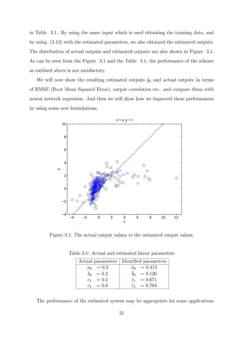
in Table 3.1. By using the same input which is used obtaining the training data, and
by using (3.13) with the estimated parameters, we also obtained the estimated outputs.
The distribution of actual outputs and estimated outputs are also shown in Figure 3.1.
As can be seen from the Figure 3.1 and the Table 3.1, the performance of the scheme
as outlined above is not satisfactory.
We will now show the resulting estimated outputs yk and actual outputs in terms
of RMSE (Root Mean Squared Error), output correlation etc. and compare them with
neural network regression. And then we will show how we improved these performances
by using some new formulations.
−4 −2 0 2 4 6 8 10 12−4
−2
0
2
4
6
8
10
x
y
x = x, y = r
Figure 3.1: The actual output values vs the estimated output values.
Table 3.1: Actual and estimated linear parameters
Actual parameters Identified parametersa0 = 0.3 a0 = 0.413
b0 = 0.2 b0 = 0.126c1 = 0.5 c1 = 0.671c2 = 0.6 c2 = 0.704
The performance of the estimated system may be appropriate for some applications
21
and may be not for some others. We will now compare these results with neural network
regression. But with neural networks we will not be able to estimate the parameters of
the linear part in (3.14). Only the inputs and outputs will be mapped and both will be
compared in terms of some performance criterions such as RMSE, correlation coefficients
etc. Regression (R) Values measure the correlation between estimated outputs and targets
(actual outputs). While an R = 1 means a close relationship, R = 0 means a random
relationship. Mean Squared Error is the average squared difference between outputs and
targets (actual outputs). Obviously lower values of RMSE indicates better performance.
3.3 Feedforward Neural Network Regression
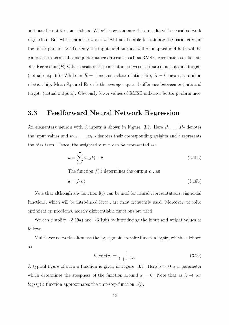
An elementary neuron with R inputs is shown in Figure 3.2. Here P1, . . . , PR denotes
the input values and w1,1, . . . , w1,R denotes their corresponding weights and b represents
the bias term. Hence, the weighted sum n can be represented as:
n =R∑i=1
w1,iPi + b (3.19a)
The function f(.) determines the output a , as
a = f(n) (3.19b)
Note that although any function f(.) can be used for neural representations, sigmoidal
functions, which will be introduced later , are most frequently used. Moreover, to solve
optimization problems, mostly differentiable functions are used.
We can simplify (3.19a) and (3.19b) by introducing the input and weight values as
follows.
Multilayer networks often use the log-sigmoid transfer function logsig, which is defined
as
logsig(n) =1
1 + e−λn(3.20)
A typical figure of such a function is given in Figure 3.3. Here λ > 0 is a parameter
which determines the steepness of the function around x = 0. Note that as λ → ∞,
logsig(.) function approximates the unit-step function 1(.).
22
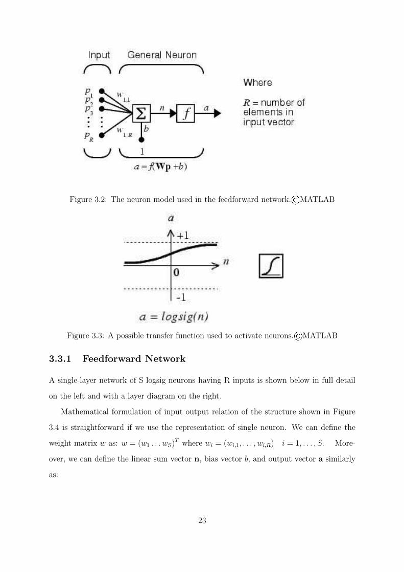
Figure 3.2: The neuron model used in the feedforward network.©MATLAB
Figure 3.3: A possible transfer function used to activate neurons.©MATLAB
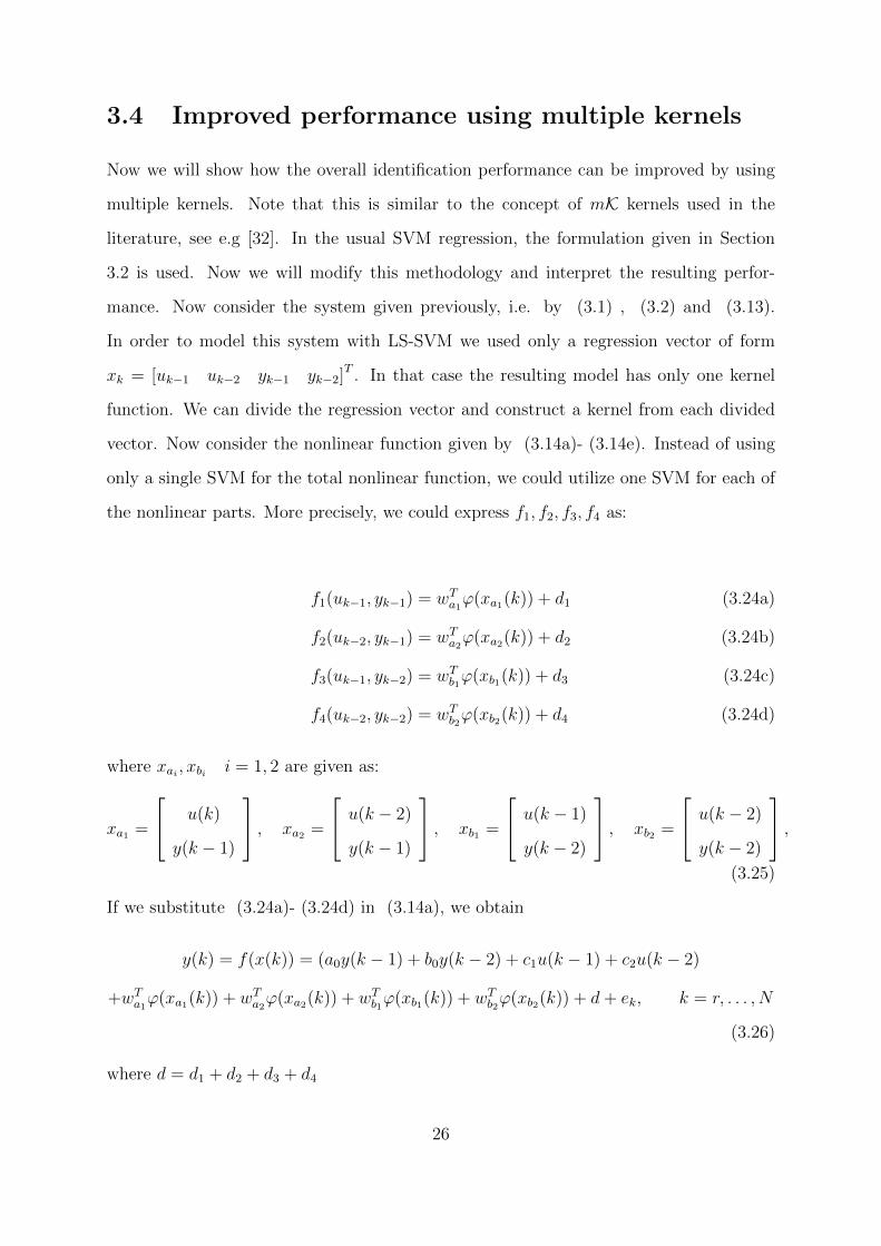
3.3.1 Feedforward Network
A single-layer network of S logsig neurons having R inputs is shown below in full detail
on the left and with a layer diagram on the right.
Mathematical formulation of input output relation of the structure shown in Figure
3.4 is straightforward if we use the representation of single neuron. We can define the
weight matrix w as: w = (w1 . . . wS)T where wi = (wi,1, . . . , wi,R) i = 1, . . . , S. More-
over, we can define the linear sum vector n, bias vector b, and output vector a similarly
as:
23
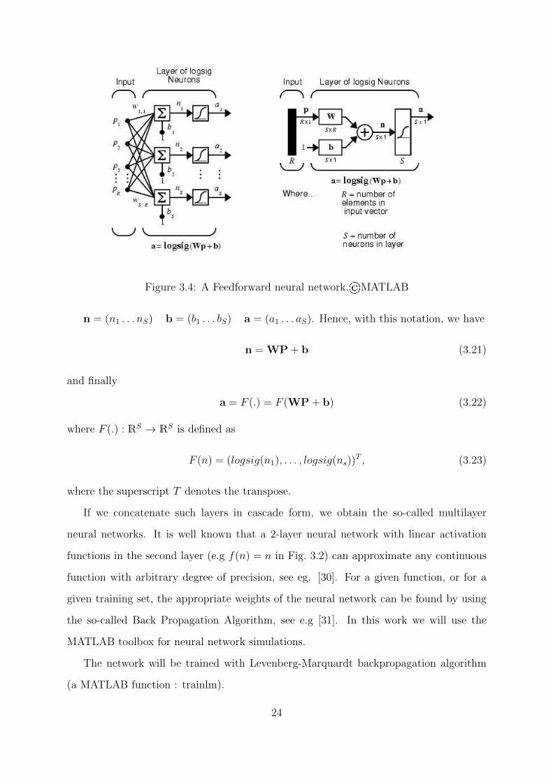
Figure 3.4: A Feedforward neural network.©MATLAB
n = (n1 . . . nS) b = (b1 . . . bS) a = (a1 . . . aS). Hence, with this notation, we have
n = WP+ b (3.21)
and finally
a = F (.) = F (WP+ b) (3.22)
where F (.) : RS → RS is defined as
F (n) = (logsig(n1), . . . , logsig(ns))T , (3.23)
where the superscript T denotes the transpose.
If we concatenate such layers in cascade form, we obtain the so-called multilayer
neural networks. It is well known that a 2-layer neural network with linear activation
functions in the second layer (e.g f(n) = n in Fig. 3.2) can approximate any continuous
function with arbitrary degree of precision, see eg. [30]. For a given function, or for a
given training set, the appropriate weights of the neural network can be found by using
the so-called Back Propagation Algorithm, see e.g [31]. In this work we will use the
MATLAB toolbox for neural network simulations.
The network will be trained with Levenberg-Marquardt backpropagation algorithm
(a MATLAB function : trainlm).
24

Figure 3.5: The actual output values vs the estimated output values using Neural Net-works.
The nonlinear system that is to be modeled is the one that we have used in the
previous section, i.e. the function (3.13). The length of the training data is N = 300,
the input used to excite the system is the same as before, i.e u(k) = N (0, 2), hence the
output is also the same in order for the comparisons be sensible. The performance results
are shown in the Figure 3.5. In the Figure 3.5 the target, i.e axis x, denote the actual
output, i.e y(k), while axis y denote the estimated output, i.e y(k). The value R denote
the correlation between actual y(k) (target) and estimated outputs y(k) (axis y).
The results show that the Neural Networks perform much better than LS-SVM Re-
gression, in terms of both RMSE and correlation (R) values. However, note that here we
do not estimate the parameters a0, . . . , c2, but estimate the input-output relation.
25
3.4 Improved performance using multiple kernels
Now we will show how the overall identification performance can be improved by using
multiple kernels. Note that this is similar to the concept of mK kernels used in the
literature, see e.g [32]. In the usual SVM regression, the formulation given in Section
3.2 is used. Now we will modify this methodology and interpret the resulting perfor-
mance. Now consider the system given previously, i.e. by (3.1) , (3.2) and (3.13).
In order to model this system with LS-SVM we used only a regression vector of form
xk = [uk−1 uk−2 yk−1 yk−2]T . In that case the resulting model has only one kernel
function. We can divide the regression vector and construct a kernel from each divided
vector. Now consider the nonlinear function given by (3.14a)- (3.14e). Instead of using
only a single SVM for the total nonlinear function, we could utilize one SVM for each of
the nonlinear parts. More precisely, we could express f1, f2, f3, f4 as:
f1(uk−1, yk−1) = wTa1ϕ(xa1(k)) + d1 (3.24a)
f2(uk−2, yk−1) = wTa2ϕ(xa2(k)) + d2 (3.24b)
f3(uk−1, yk−2) = wTb1ϕ(xb1(k)) + d3 (3.24c)
f4(uk−2, yk−2) = wTb2ϕ(xb2(k)) + d4 (3.24d)
where xai , xbi i = 1, 2 are given as:
xa1 =
u(k)
y(k − 1)
, xa2 =
u(k − 2)
y(k − 1)
, xb1 =
u(k − 1)
y(k − 2)
, xb2 =
u(k − 2)
y(k − 2)
,
(3.25)
If we substitute (3.24a)- (3.24d) in (3.14a), we obtain
y(k) = f(x(k)) = (a0y(k − 1) + b0y(k − 2) + c1u(k − 1) + c2u(k − 2)
+wTa1ϕ(xa1(k)) + wT
a2ϕ(xa2(k)) + wT
b1ϕ(xb1(k)) + wT
b2ϕ(xb2(k)) + d+ ek, k = r, . . . , N
(3.26)
where d = d1 + d2 + d3 + d4
26
As seen in the above equation instead of only one SVM , 4 SVM are used to model
the function f(.). To obtain the optimal points, the optimization problem is constructed
as follows:
minwx,ξk
F (w, ξk) = 1/2∑x
wTxwx + γ/2
N∑
k=r
ξ2k
subject to y(k) = f(x(k)) = (a0y(k − 1) + b0y(k − 2) + c1u(k − 1) + c2u(k − 2)
+wTa1ϕ(xa1(k)) + wT
a2ϕ(xa2(k)) + wT
b1ϕ(xb1(k)) + wT
b2ϕ(xb2(k)) + d+ ξk,
k = r, . . . , N (3.27a)
N∑
k=1
wTxϕ(xx(k)) = 0 for x = a1, a2, b1, b2. (3.27b)
The problem is quadratic and the associated lagrangian can be given as:
L (w, a,b, c, d, ξk, α, β) = F (w, ξk)−N∑
k=r
αk(a0y(k − 1) + b0y(k − 2) + c1u(k − 1)+
c2u(k − 2) + wTa1ϕ(xa1(k))+wT
a2ϕ(xa2(k)) + wT
b1ϕ(xb1(k)) + wT
b2ϕ(xb2(k)) + d+ ξk − yk)
−∑
x=a0,b0,c1,c2
βx
N∑
k=1
wTxϕ(xx(k)) (3.28)
Again by using the Karush-Kuhn-Tucker (KKT) conditions we obtain the following
equations.
∂L
∂wx
= 0 → wx =N∑
k=r
αkϕ(xk) + βx
N∑
k=1
ϕ(xk), x = a0, b0, c1, c2 (3.29a)
∂L
∂a0, b0, c1, c2= 0 →
N∑
k=r
αky(k − i) = 0, i = 1, 2.N∑
k=r
αku(k − i) = 0 i = 1, 2
(3.29b)
∂L
∂d= 0 →
N∑
k=r
αk = 0 (3.29c)
∂L
∂ek= 0 → αk = γξk, k = r, . . . , N (3.29d)
∂L
∂αk
= 0 → (3.27a) (3.29e)
∂L
∂βk
= 0 →N∑
k=1
wTxϕ(xx(k)) = 0 for x = a1, a2, b1, b2. (3.29f)
27
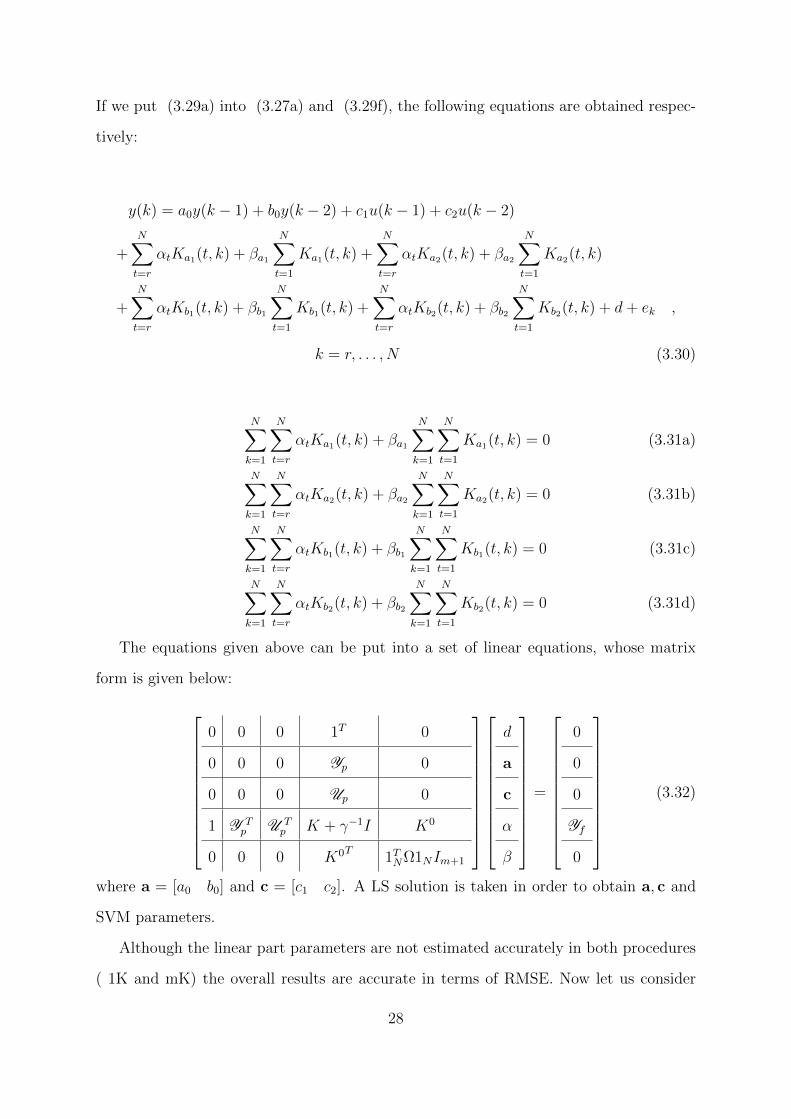
If we put (3.29a) into (3.27a) and (3.29f), the following equations are obtained respec-
tively:
y(k) = a0y(k − 1) + b0y(k − 2) + c1u(k − 1) + c2u(k − 2)
+N∑t=r
αtKa1(t, k) + βa1
N∑t=1
Ka1(t, k) +N∑t=r
αtKa2(t, k) + βa2
N∑t=1
Ka2(t, k)
+N∑t=r
αtKb1(t, k) + βb1
N∑t=1
Kb1(t, k) +N∑t=r
αtKb2(t, k) + βb2
N∑t=1
Kb2(t, k) + d+ ek ,
k = r, . . . , N (3.30)
N∑
k=1
N∑t=r
αtKa1(t, k) + βa1
N∑
k=1
N∑t=1
Ka1(t, k) = 0 (3.31a)
N∑
k=1
N∑t=r
αtKa2(t, k) + βa2
N∑
k=1
N∑t=1
Ka2(t, k) = 0 (3.31b)
N∑
k=1
N∑t=r
αtKb1(t, k) + βb1
N∑
k=1
N∑t=1
Kb1(t, k) = 0 (3.31c)
N∑
k=1
N∑t=r
αtKb2(t, k) + βb2
N∑
k=1
N∑t=1
Kb2(t, k) = 0 (3.31d)
The equations given above can be put into a set of linear equations, whose matrix
form is given below:
0 0 0 1T 0
0 0 0 Yp 0
0 0 0 Up 0
1 Y Tp U T
p K + γ−1I K0
0 0 0 K0T 1TNΩ1NIm+1
d
a
c
α
β
=
0
0
0
Yf
0
(3.32)
where a = [a0 b0] and c = [c1 c2]. A LS solution is taken in order to obtain a, c and
SVM parameters.
Although the linear part parameters are not estimated accurately in both procedures
( 1K and mK) the overall results are accurate in terms of RMSE. Now let us consider
28
0 5 10
−5
0
5
10
15
x
y
x = x, y = r
0 5 10
−5
0
5
10
15
x
y
x = x, y = r
Figure 3.6: The corrleation between actual and estimated output. Left using LS-SVR,right using LS-SVR mK.
the example given by (3.13) again with the actual parameters chosen the same as a0 =
0.3, b0 = 0.2, c1 = 0.5, c2 = 0.6. with these parameters we simulated the system
given by (3.1) , (3.2), (3.13) by using input as a random signal of Gaussian distribution
with 0 mean and standard deviation 2. We created N = 300 samples of training data.
Noise also has a Gaussian distribution of 0 mean and standard deviation less than 0.2.
Then by solving (3.32), we obtained the estimated parameters as shown in Table 3.2.
By using the same input which is used obtaining the training data, and by using (3.13)
with the estimated parameters, we also obtained the estimated outputs. The distribution
of actual outputs and estimated outputs are also shown in Figure 3.7. As can be seen
from the Figure 3.7, the performance of the scheme as outlined above is satisfactory.
Finally to further signify the effectiveness of using LS-SVR mK some performance
comparisons are shown in the Tables 3.3, 3.4 and 3.5. As can be seen from the
tables the LS-SVR mK and neural network regression performs much better than the
conventional LS-SVR regression. If we compare LS-SVR mK and neural networks , each
29
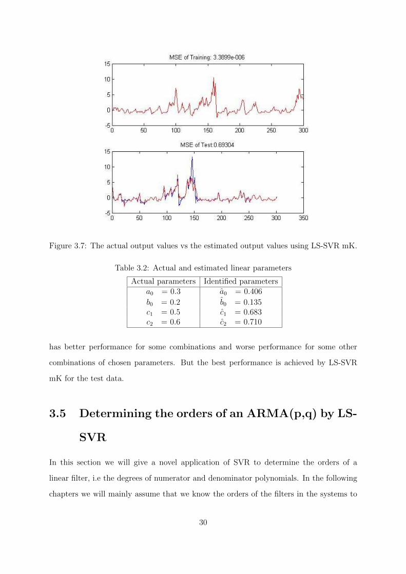
Figure 3.7: The actual output values vs the estimated output values using LS-SVR mK.
Table 3.2: Actual and estimated linear parameters
Actual parameters Identified parametersa0 = 0.3 a0 = 0.406
b0 = 0.2 b0 = 0.135c1 = 0.5 c1 = 0.683c2 = 0.6 c2 = 0.710
has better performance for some combinations and worse performance for some other
combinations of chosen parameters. But the best performance is achieved by LS-SVR
mK for the test data.
3.5 Determining the orders of an ARMA(p,q) by LS-
SVR
In this section we will give a novel application of SVR to determine the orders of a
linear filter, i.e the degrees of numerator and denominator polynomials. In the following
chapters we will mainly assume that we know the orders of the filters in the systems to
30
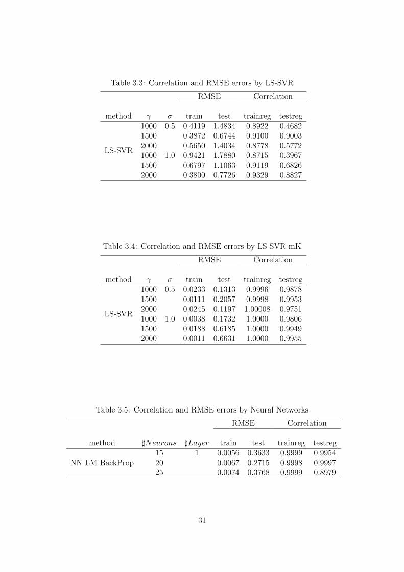
Table 3.3: Correlation and RMSE errors by LS-SVR
RMSE Correlation
method γ σ train test trainreg testreg
LS-SVR
1000 0.5 0.4119 1.4834 0.8922 0.46821500 0.3872 0.6744 0.9100 0.90032000 0.5650 1.4034 0.8778 0.57721000 1.0 0.9421 1.7880 0.8715 0.39671500 0.6797 1.1063 0.9119 0.68262000 0.3800 0.7726 0.9329 0.8827
Table 3.4: Correlation and RMSE errors by LS-SVR mK
RMSE Correlation
method γ σ train test trainreg testreg
LS-SVR
1000 0.5 0.0233 0.1313 0.9996 0.98781500 0.0111 0.2057 0.9998 0.99532000 0.0245 0.1197 1.00008 0.97511000 1.0 0.0038 0.1732 1.0000 0.98061500 0.0188 0.6185 1.0000 0.99492000 0.0011 0.6631 1.0000 0.9955
Table 3.5: Correlation and RMSE errors by Neural Networks
RMSE Correlation
method ]Neurons ]Layer train test trainreg testreg
NN LM BackProp15 1 0.0056 0.3633 0.9999 0.995420 0.0067 0.2715 0.9998 0.999725 0.0074 0.3768 0.9999 0.8979
31

be identified, i.e we assume that we know the number nu and ny in (3.2). There are
various ways to determine the orders of the filter in the literature, [33]. In the sequel we
will give a novel way to determine these orders. We will use LS-SVR to determine these
orders. Our method is based on a trial and error technique. The order for which the
error is least will be taken as the correct order. The AR (i.e ny in 3.2) and MA orders
(i.e nu in 3.2) are determined separately. Consider an arma(p,q) filter given as follows:
yk =
p∑i=1
aiyk−i +
q∑j=0
bjuk−j (3.33)
The aim is to determine the values of p which is AR(Auto-Regressive) order and
q which is MA(Moving-Average) order. By using LS-SVR we can train support vectors
such that the input and output training data uk, ykNk=1 are mapped with the least error.
We can train SVR in various ways. The difference is the order of the training vector xk,
where xk is as defined before
x(k) =
y(k − 1)
...
y(k − ny)
u(k)
...
u(k − nu)
(3.34)
The filter will be modeled as in (3.35), similar to the mapping in (3.4).
y(xk) =< w,ϕ(xk) > +d = wTϕ(xk) + d, (3.35)
For a training data uk, yk, we may construct the following optimization problem.
minw,ξ
F (w, ξk) = 1/2‖w‖2 + γ/2∑
ξ2k (3.36)
subject to yk = wTϕ(xk) + d+ ξk, ∀k = 1, . . . , N
We will mainly change the lags ny and nu and compare the errors between the actual and
estimated outputs. Note that the lag nu can be considered to be related to the order q,
whereas the lag ny can be considered to be related to the order p.
32

The solution to the optimization problem (3.36) is the same as the solution (3.9) in
section 3.2. The resulting estimated outputs can be given as :
yk =N∑t=1
αkK(xt, xk) + d (3.37)
At the first iteration the lag nu is set to 0, i.e only the current input is present in the
regression vector xk, whereas the lag ny is increased by 1 for each training iteration. The
MSE (Mean Squared Error ) between the actual yk and yk is computed. As can be seen
from the Figure 3.8, the error is maximum for the lag ny = 1, then it decreases up to
the lag ny = 6, which is the true order, i.e p = 6, then it increases. To obtain the order
q, i.e numerator order, a similar approach is applied. The lag ny is taken to be 0 at
first iteration, the lag nu is increased starting from nu = 1 at first iteration. The errors
between actual yk and yk are computed, the lag for which the error is minimum is taken
to be true order. This can be seen from the Figure 3.9. The true order is 3 and the error
is minimum at that point. So in this way the order of the filter is obtained correctly.
Figure 3.8: The normalized error between actual and estimated outputs as the lagsincreases.
Various input signals are used to see the best results. Choosing input as a signal of
uniform distribution between some points [p1, p2] did not give accurate results. The best
results are obtained when the input signal is chosen to be a random variable of normal
distribution.
In order to obtain the numerator order i.e.q) more attention is required. The regression
vector is composed of only input values. For the previous case the lag for input was chosen
33
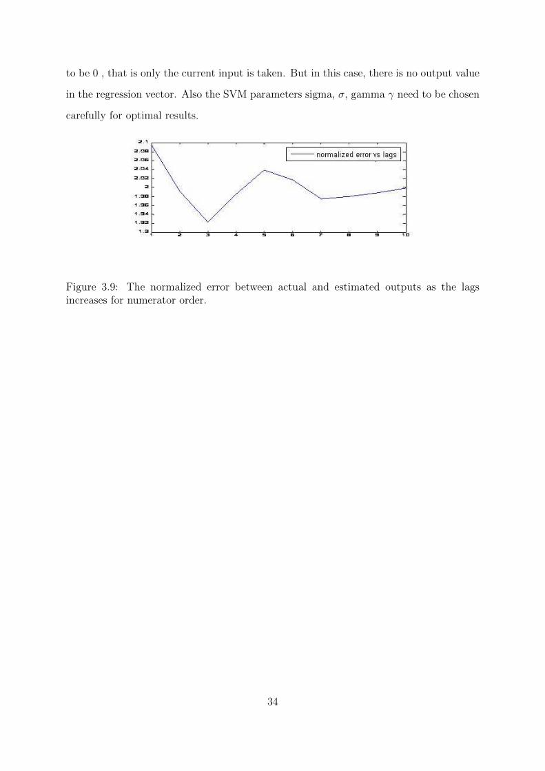
to be 0 , that is only the current input is taken. But in this case, there is no output value
in the regression vector. Also the SVM parameters sigma, σ, gamma γ need to be chosen
carefully for optimal results.
Figure 3.9: The normalized error between actual and estimated outputs as the lagsincreases for numerator order.
34
Chapter 4
IDENTIFICATION AND
CONTROL OF WIENER
SYSTEMS BY LS-SVM
In this chapter we will first show how a method which utilizes LS-SVM for the identifi-
cation of Hammerstein systems. We then propose a novel method when the nonlinearity
in Hammerstein systems has a finite memory. We will then give some results on Wiener
systems when the same procedure used for identification of Hammerstein systems is ap-
plied. Then we will develop our own methodology to improve the performance of the
identification of Wiener systems. We then propose a novel method for the control of
Wiener systems. Finally we will make comparisons between performances of all these
procedures.
4.1 Hammerstein Model Identification Using LS-SVM
In this section we will briefly explain how Hammerstein models can be identified by
using LS-SVM. In the following sections we will explain how the method proposed in
Chapter 2 can be used for the identification of Hammerstein type systems and how it
can be modified for the identification of Wiener type systems . The block diagram of a
35
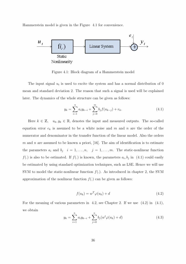
Hammerstein model is given in the Figure 4.1 for convenience.
Figure 4.1: Block diagram of a Hammerstein model
The input signal ut is used to excite the system and has a normal distribution of 0
mean and standard deviation 2. The reason that such a signal is used will be explained
later. The dynamics of the whole structure can be given as follows:
yk =n∑
i=1
aiyk−i +m∑j=0
bjf(uk−j) + ek. (4.1)
Here k ∈ Z, uk, yk ∈ R, denotes the input and measured outputs. The so-called
equation error ek is assumed to be a white noise and m and n are the order of the
numerator and denominator in the transfer function of the linear model. Also the orders
m and n are assumed to be known a priori, [16]. The aim of identification is to estimate
the parameters ai and bj i = 1, . . . , n, j = 1, . . . ,m. The static-nonlinear function
f(.) is also to be estimated. If f(.) is known, the parameters ai, bj in (4.1) could easily
be estimated by using standard optimization techniques, such as LSE. Hence we will use
SVM to model the static-nonlinear function f(.). As introduced in chapter 2, the SVM
approximation of the nonlinear function f(.) can be given as follows:
f(uk) = wTϕ(uk) + d (4.2)
For the meaning of various parameters in 4.2, see Chapter 2. If we use (4.2) in (4.1),
we obtain
yk =n∑
i=1
aiyk−i +n∑
j=0
bj(wtϕ(uk) + d) (4.3)
36
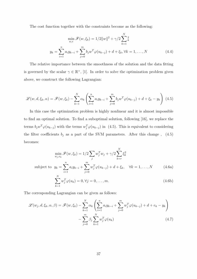
The cost function together with the constraints become as the following:
minw,e
F (w, ξk) = 1/2‖w‖2 + γ/2N∑
k=1
2k
yk =n∑
i=1
aiyk−i +m∑j=0
bjwTϕ(uk−j) + d+ ξk,∀k = 1, . . . , N (4.4)
The relative importance between the smoothness of the solution and the data fitting
is governed by the scalar γ ∈ R+, [1]. In order to solve the optimization problem given
above, we construct the following Lagrangian:
L (w, d, ξk, α) = F (w, ξk)−N∑
k=1
αk
(n∑
i=1
aiyk−i +m∑j=0
bjwTϕ(uk−j) + d+ ξk − yk
)(4.5)
In this case the optimization problem is highly nonlinear and it is almost impossible
to find an optimal solution. To find a suboptimal solution, following [16], we replace the
terms bjwTϕ(uk−j) with the terms wT
j ϕ(uk−j) in (4.5). This is equivalent to considering
the filter coefficients bj as a part of the SVM parameters. After this change , (4.5)
becomes:
minwj ,ek
F (w, ξk) = 1/2∑j
wTj wj + γ/2
N∑
k=r
ξ2k
subject to yk =n∑
i=1
aiyk−i +m∑j=0
wTj ϕ(uk−j) + d+ ξk, ∀k = 1, . . . , N (4.6a)
N∑
k=1
wTj ϕ(uk) = 0,∀j = 0, . . . ,m. (4.6b)
The corresponding Lagrangian can be given as follows:
L (wj, d, ξk, α, β) = F (w, ξk)−N∑
k=1
αk
(n∑
i=1
aiyk−i +m∑j=0
wTj ϕ(uk−j) + d+ ek − yk
)
−m∑j=0
βj
N∑
k=1
wTj ϕ(uk) (4.7)
37
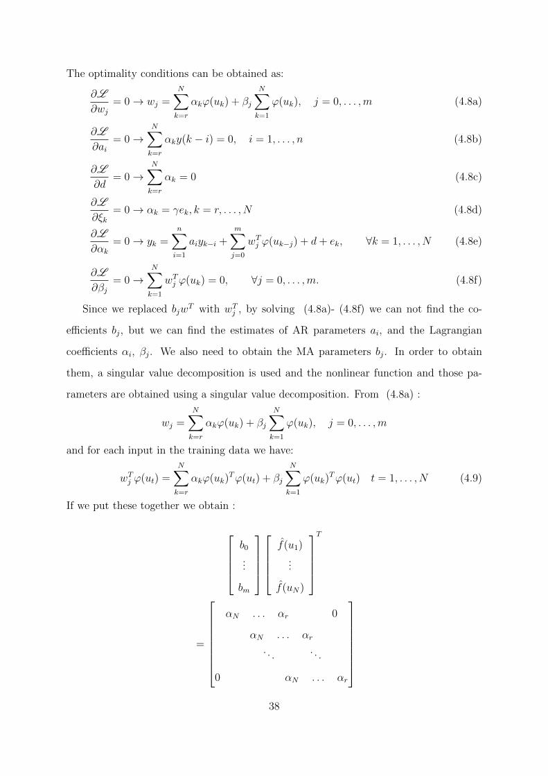
The optimality conditions can be obtained as:
∂L
∂wj
= 0 → wj =N∑
k=r
αkϕ(uk) + βj
N∑
k=1
ϕ(uk), j = 0, . . . ,m (4.8a)
∂L
∂ai= 0 →
N∑
k=r
αky(k − i) = 0, i = 1, . . . , n (4.8b)
∂L
∂d= 0 →
N∑
k=r
αk = 0 (4.8c)
∂L
∂ξk= 0 → αk = γek, k = r, . . . , N (4.8d)
∂L
∂αk
= 0 → yk =n∑
i=1
aiyk−i +m∑j=0
wTj ϕ(uk−j) + d+ ek, ∀k = 1, . . . , N (4.8e)
∂L
∂βj
= 0 →N∑
k=1
wTj ϕ(uk) = 0, ∀j = 0, . . . ,m. (4.8f)
Since we replaced bjwT with wT
j , by solving (4.8a)- (4.8f) we can not find the co-
efficients bj, but we can find the estimates of AR parameters ai, and the Lagrangian
coefficients αi, βj. We also need to obtain the MA parameters bj. In order to obtain
them, a singular value decomposition is used and the nonlinear function and those pa-
rameters are obtained using a singular value decomposition. From (4.8a) :
wj =N∑
k=r
αkϕ(uk) + βj
N∑
k=1
ϕ(uk), j = 0, . . . ,m
and for each input in the training data we have:
wTj ϕ(ut) =
N∑
k=r
αkϕ(uk)Tϕ(ut) + βj
N∑
k=1
ϕ(uk)Tϕ(ut) t = 1, . . . , N (4.9)
If we put these together we obtain :
b0...
bm
f(u1)
...
f(uN)
T
=
αN . . . αr 0
αN . . . αr
. . . . . .
0 αN . . . αr
38
×
ΩN,1 ΩN,2 . . .ΩN,N
ΩN−1,1 ΩN−1,2 . . .ΩN−1,N
......
...
Ωr−m,1 Ωr−m,2 . . .Ωr−m,N
+
β0
...
βm
N∑t=1
Ωt,1
...
Ωt,N
T
(4.10)
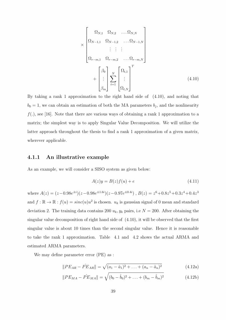
By taking a rank 1 approximation to the right hand side of (4.10), and noting that
b0 = 1, we can obtain an estimation of both the MA parameters bj, and the nonlinearity
f(.), see [16]. Note that there are various ways of obtaining a rank 1 approximation to a
matrix; the simplest way is to apply Singular Value Decomposition. We will utilize the
latter approach throughout the thesis to find a rank 1 approximation of a given matrix,
wherever applicable.
4.1.1 An illustrative example
As an example, we will consider a SISO system as given below:
A(z)y = B(z)f(u) + e (4.11)
where A(z) = (z−0.98e±i)(z−0.98e±1.6i)(z−0.97e±0.4i) , B(z) = z6+0.8z5+0.3z4+0.4z3
and f : R→ R : f(u) = sinc(u)u2 is chosen. uk is gaussian signal of 0 mean and standard
deviation 2. The training data contains 200 uk, yk pairs, i.e N = 200. After obtaining the
singular value decomposition of right hand side of (4.10), it will be observed that the first
singular value is about 10 times than the second singular value. Hence it is reasonable
to take the rank 1 approximation. Table 4.1 and 4.2 shows the actual ARMA and
estimated ARMA parameters.
We may define parameter error (PE) as :
‖PEAR − PEAR‖ =√
(a1 − a1)2 + . . .+ (an − an)2 (4.12a)
‖PEMA − PEMA‖ =
√(b0 − b0)2 + . . .+ (bm − bm)2 (4.12b)
39
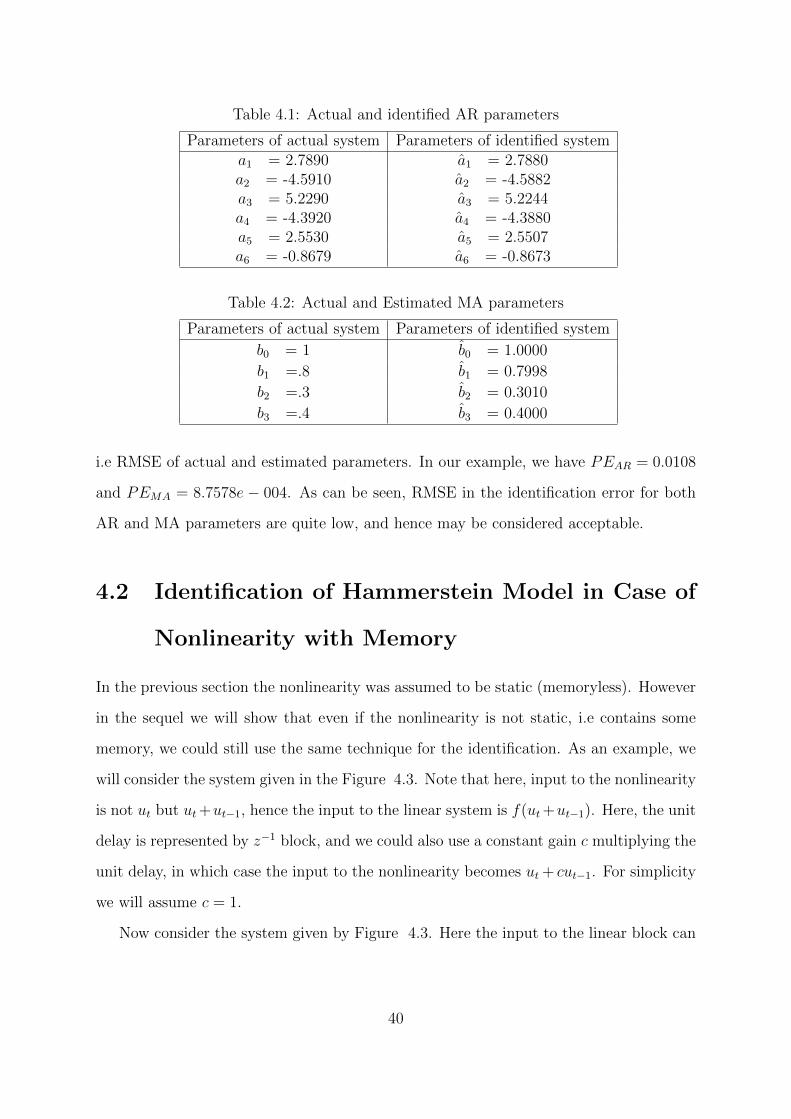
Table 4.1: Actual and identified AR parameters
Parameters of actual system Parameters of identified systema1 = 2.7890 a1 = 2.7880a2 = -4.5910 a2 = -4.5882a3 = 5.2290 a3 = 5.2244a4 = -4.3920 a4 = -4.3880a5 = 2.5530 a5 = 2.5507a6 = -0.8679 a6 = -0.8673
Table 4.2: Actual and Estimated MA parameters
Parameters of actual system Parameters of identified system
b0 = 1 b0 = 1.0000
b1 =.8 b1 = 0.7998
b2 =.3 b2 = 0.3010
b3 =.4 b3 = 0.4000
i.e RMSE of actual and estimated parameters. In our example, we have PEAR = 0.0108
and PEMA = 8.7578e − 004. As can be seen, RMSE in the identification error for both
AR and MA parameters are quite low, and hence may be considered acceptable.
4.2 Identification of Hammerstein Model in Case of
Nonlinearity with Memory
In the previous section the nonlinearity was assumed to be static (memoryless). However
in the sequel we will show that even if the nonlinearity is not static, i.e contains some
memory, we could still use the same technique for the identification. As an example, we
will consider the system given in the Figure 4.3. Note that here, input to the nonlinearity
is not ut but ut+ut−1, hence the input to the linear system is f(ut+ut−1). Here, the unit
delay is represented by z−1 block, and we could also use a constant gain c multiplying the
unit delay, in which case the input to the nonlinearity becomes ut + cut−1. For simplicity
we will assume c = 1.
Now consider the system given by Figure 4.3. Here the input to the linear block can
40
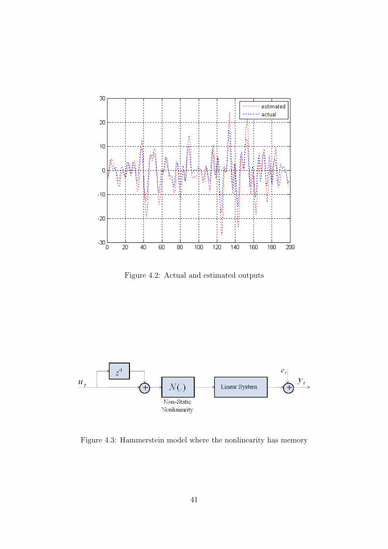
Figure 4.2: Actual and estimated outputs
Figure 4.3: Hammerstein model where the nonlinearity has memory
41
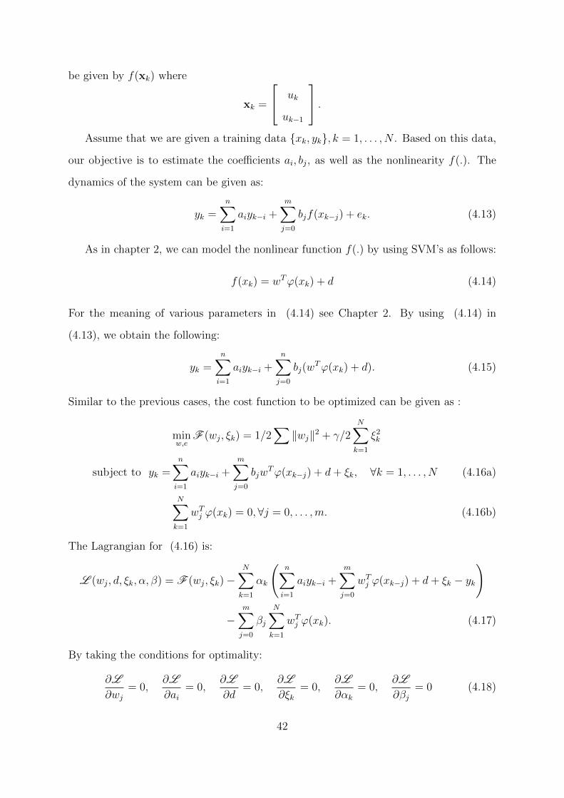
be given by f(xk) where
xk =
uk
uk−1
.
Assume that we are given a training data xk, yk, k = 1, . . . , N . Based on this data,
our objective is to estimate the coefficients ai, bj, as well as the nonlinearity f(.). The
dynamics of the system can be given as:
yk =n∑
i=1
aiyk−i +m∑j=0
bjf(xk−j) + ek. (4.13)
As in chapter 2, we can model the nonlinear function f(.) by using SVM’s as follows:
f(xk) = wTϕ(xk) + d (4.14)
For the meaning of various parameters in (4.14) see Chapter 2. By using (4.14) in
(4.13), we obtain the following:
yk =n∑
i=1
aiyk−i +n∑
j=0
bj(wTϕ(xk) + d). (4.15)
Similar to the previous cases, the cost function to be optimized can be given as :
minw,e
F (wj, ξk) = 1/2∑
‖wj‖2 + γ/2N∑
k=1
ξ2k
subject to yk =n∑
i=1
aiyk−i +m∑j=0
bjwTϕ(xk−j) + d+ ξk, ∀k = 1, . . . , N (4.16a)
N∑
k=1
wTj ϕ(xk) = 0,∀j = 0, . . . ,m. (4.16b)
The Lagrangian for (4.16) is:
L (wj, d, ξk, α, β) = F (wj, ξk)−N∑
k=1
αk
(n∑
i=1
aiyk−i +m∑j=0
wTj ϕ(xk−j) + d+ ξk − yk
)
−m∑j=0
βj
N∑
k=1
wTj ϕ(xk). (4.17)
By taking the conditions for optimality:
∂L
∂wj
= 0,∂L
∂ai= 0,
∂L
∂d= 0,
∂L
∂ξk= 0,
∂L
∂αk
= 0,∂L
∂βj
= 0 (4.18)
42
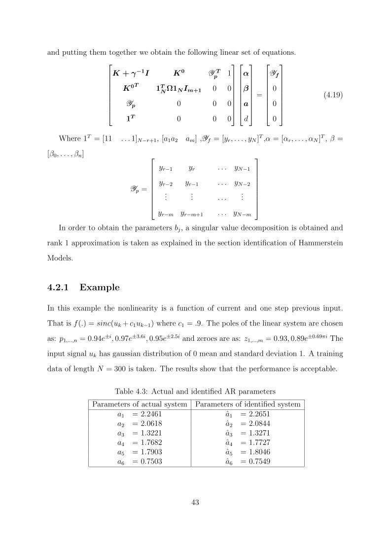
and putting them together we obtain the following linear set of equations.
K + γ−1I K0 Y Tp 1
K0T 1TNΩ1NIm+1 0 0
Yp 0 0 0
1T 0 0 0
α
β
a
d
=
Yf
0
0
0
(4.19)
Where 1T = [11 . . . 1]N−r+1, [a1a2 am] ,Yf = [yr, . . . , yN ]T ,α = [αr, . . . , αN ]
T , β =
[β0, . . . , βn]
Yp =
yr−1 yr . . . yN−1
yr−2 yr−1 . . . yN−2
...... . . .
...
yr−m yr−m+1 . . . yN−m
In order to obtain the parameters bj, a singular value decomposition is obtained and
rank 1 approximation is taken as explained in the section identification of Hammerstein
Models.
4.2.1 Example
In this example the nonlinearity is a function of current and one step previous input.
That is f(.) = sinc(uk + c1uk−1) where c1 = .9. The poles of the linear system are chosen
as: p1,...,n = 0.94e±i, 0.97e±3.6i, 0.95e±2.5i and zeroes are as: z1,...,m = 0.93, 0.89e±0.69πi The
input signal uk has gaussian distribution of 0 mean and standard deviation 1. A training
data of length N = 300 is taken. The results show that the performance is acceptable.
Table 4.3: Actual and identified AR parameters
Parameters of actual system Parameters of identified systema1 = 2.2461 a1 = 2.2651a2 = 2.0618 a2 = 2.0844a3 = 1.3221 a3 = 1.3271a4 = 1.7682 a4 = 1.7727a5 = 1.7903 a5 = 1.8046a6 = 0.7503 a6 = 0.7549
43

Table 4.4: Actual and Estimated MA parameters
Parameters of actual system Parameters of identified system
b0 = 1.000 b0 = 1.0000
b1 =-0.2251 b1 = -0.2306
b2 = 0.1332 b2 = 0.1416
b3 =-0.7382 b3 = -0.7320
The RMSE between actual and estimated parameters are :PEAR = 0.0073 and
PEMA = 0.0118. The numerator parameters are estimated a little worse than the case of
the static-nonlinearity. This might be due to the fact the output of the system is highly
oscillatory. Moreover, after obtaining rank 1 approximation of the right hand side of
equivalent matrix (4.10), the first singular value is 3 to 4 times larger than the second
singular value. In the case that the nonlinearity was static , the first singular value was
about 10 times larger than the second singular value. Hence rank 1 approximation leads
more error in the case the nonlinearity has some memory.
Since the nonlinearity is a function of a two dimensional vector , namely xk, we can
still visualize the nonlinearity modeled by SVM, which is shown in the Figure 4.4.
−3−2
−10
12
3−2
0
2−2
−1
0
1
2
u(k−1)
Nonlinearity with memory: f(.)= sinc(u + .9*us).*(u +.9*us)
u(k)
y(k)
Actual nonlinearityEstimated nonlinearity
Figure 4.4: The actual and estimated nonlinear function. RMSE = 0.8402
44
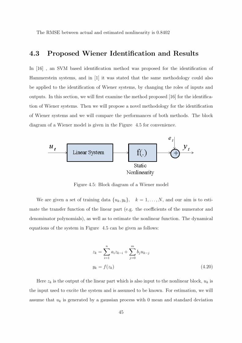
The RMSE between actual and estimated nonlinearity is 0.8402
4.3 Proposed Wiener Identification and Results
In [16] , an SVM based identification method was proposed for the identification of
Hammerstein systems, and in [1] it was stated that the same methodology could also
be applied to the identification of Wiener systems, by changing the roles of inputs and
outputs. In this section, we will first examine the method proposed [16] for the identifica-
tion of Wiener systems. Then we will propose a novel methodology for the identification
of Wiener systems and we will compare the performances of both methods. The block
diagram of a Wiener model is given in the Figure 4.5 for convenience.
Figure 4.5: Block diagram of a Wiener model
We are given a set of training data uk, yk, k = 1, . . . , N , and our aim is to esti-
mate the transfer function of the linear part (e.g. the coefficients of the numerator and
denominator polynomials), as well as to estimate the nonlinear function. The dynamical
equations of the system in Figure 4.5 can be given as follows:
zk =n∑
i=1
aizk−i +m∑j=0
bjuk−j
yk = f(zk) (4.20)
Here zk is the output of the linear part which is also input to the nonlinear block, uk is
the input used to excite the system and is assumed to be known. For estimation, we will
assume that uk is generated by a gaussian process with 0 mean and standard deviation
45

is taken to be 2; ek is also assumed to be a gaussian noise where magnitude is at most
10 percent of the input signal. Both uk and ek are assumed to be independent. In [1]
it is proposed that by considering the outputs of the model as inputs and the inputs as
outputs, the method used to identify Hammerstein systems can be applied to identify the
Wiener systems assuming that the static nonlinearity is invertible. In the sequel, we will
use this methodology in an example and examine its performance.
Following the methodology mentioned above, we may obtain the following relation
between uk and yk.
uk =m∑i=1
biuk−i +n∑
j=1
wTj ϕ(yk−j) + d+ ξk, ∀k = 1, . . . , N (4.21)
The cost function together with the constraints become as the following:
minw,ξk
F (w, ξk) = 1/2‖w‖2 + γ/2N∑
k=1
ξ2k
uk =m∑i=1
biuk−i +n∑
j=1
wTj ϕ(yk−j) + d+ ξk, ∀k = 1, . . . , N (4.22)
L (w, d, ξk, α) = F (w, ξk)−N∑
k=1
αk
(m∑i=1
biuk−i +n∑
j=0
wTj ϕ(yk−j) + d+ ξk − uk
)(4.23)
Note that here the training data uk, yk is taken from the Wiener system given by
(4.20), and hence yk also contains the measurement noise. The optimization problem is
similar to the optimization problem for identification of Hammerstein models. Following
the steps as given in (sec 2), i.e. taking derivative of Lagrangian w.r.t all of its vari-
ables and setting them to zero, we obtain the following linear set of equations for the
identification of Wiener systems:
0 0 1T 0
0 0 Up 0
1 U Tp K+ γ−1I K0
0 0 K0T 1TNΩ1NIm+1
d
b
α
β
=
0
0
Uf
0
(4.24)
46

where 1T = [1 1 . . . 1]N−r+1, b = [b1 b2 bm] ,Uf = [ur, . . . , uN ]T , α = [αr, . . . , αN ]
T ,
β = [β0, . . . , βn]
Up =
ur−1 ur . . . uN−1
ur−2 ur−1 . . . uN−2
...... . . .
...
ur−m ur−m+1 . . . uN−m
(4.25)
Ωi,j = K(yi, yj) = ϕ(yi)Tϕ(yj) = e(−‖yi−yj‖2) ,K (p, q) =
∑ni=0Ωp+r−i−1,q+r−i−1,
K0(p, q) =∑N
t=1Ωt,r+p−q.
4.3.1 Example
To test the methodology given above, we consider the following example. The filter is
given as before as H(z−1) = B(z−1)/A(z−1), where B(z−1) = b0 + b1z−1 + b2z
−2 + b0z−3,
A(z−1) = a0 + a1z−1+ . . .+ anz
−n, and the parameters are chosen as given in Tables 4.5
and 4.6. The nonlinearity is chosen as a simple gain, i.e., 5. This is actually a linear
system and is one of the simplest case that can be encountered. For training, we chose
the input as a random signal that has a Gaussian distribution of 0 mean and standard
deviation 2. The measurement noise is assumed to has a Gaussian distribution of 0
mean and standard deviation 0.2. We obtained N = 200 samples of input and output
pairs uk, yk. A least squares solution of (4.24) is taken and the parameters a will
be the filter’s numerator. Finally a singular value decomposition is used to obtain the
nonlinear function the denominator parameters b as in the following equation. A rank 1
approximation of the equation is taken and the resulting column vector is b parameters,
the row vector is a model of the nonlinearity, as explained in the previous section.
a0...
an
f(u1)
...
f(uN)
T
47

=
αN . . . αr 0
αN . . . αr
. . . . . .
0 αN . . . αr
×
ΩN,1 ΩN,2 . . .ΩN,N
ΩN−1,1 ΩN−1,2 . . .ΩN−1,N
......
...
Ωr−n,1 Ωr−n,2 . . .Ωr−n,N
+
β0
...
βn
N∑t=1
Ωt,1
...
Ωt,N
T
(4.26)
Table 4.5 shows the actual and estimated parameters.
Table 4.5: Actual and identified AR parameters
Parameters of actual system Parameters of identified systema1 = 2.0900 a1 = 2.8400a2 = -2.0630 a2 = -5.6821a3 = 1.2090 a3 = 1.7784a4 = -0.4656 a4 = 4.9684a5 = 0.1164 a5 = -5.5828a6 = -0.0297 a6 = 2.4112
Table 4.6: Actual and Estimated MA parameters
Parameters of actual system Parameters of identified system
b0 = 1 b0 = 1.0000
b1 =.8 b1 = 1.0e+009 2.2078
b2 =.3 b2 = 1.0e+009 2.9717
b3 =.4 b3 = 1.0e+009 1.2305
As it is seen from the tables 4.5 and 4.6 the results are not even close to be optimal.
Besides the output is assumed to be measured without noise which is impossible in real
world applications. The assumption was that if the nonlinearity is invertible the same
procedure used to identify Hammerstein models can be used to identify Wiener models
48
too just by changing the role of inputs and outputs. The nonlinearity used is a piecewise
nonlinear function and is invertible. However, the parameter errors are very large as
compared to the previous methods. In the sequel, we will first discuss the possible reasons
for this unacceptably low performance. Then we will propose a novel identification scheme
for Wiener systems and compare the performances of both methods.
Now, assume that the training data uk, yk, k = 1, . . . , N is obtained from aWiener
system as shown in Figure 4.5. Let us assume that the linear part is given by a transfer
function H(z) = n(z)/d(z), where the degree of the numerator polynomial is m and
the denominator polynomial is n and the nonlinear part is given by a function f(.).
Furthermore, assume that m < n. If we interchange the roles of inputs and outputs, we
may view the new system as a Hammerstein system, as given by Figure 4.1. In this case,
the training data for the Hammerstein will be yk, uk, k = 1, . . . , N . The linear part in
Figure 4.1 will be given by a transfer function H(z), and the nonlinear part will be given
by a nonlinear function f(.). Obviously, we will have f(.) = f−1(.) and H(z) = H−1(z).
It appears that the invertibility of the nonlinear function f(.) is quite important for the
proposed scheme. Since in the equivalent Hammerstein model, the linear part is given by
H(z) = H−1(z). and H(z) = d(z)/n(z), where n > m, the new transfer function H(z)
becomes non-proper. Since the input to H(z) is the output of the original Wiener system,
which is corrupted by noise , one may assume that non-properness of H(z) may be the
reason for this poor estimation results. To test this we performed various simulations.
First we assumed f(.) = 1(.) i.e the identity function as shown in Figure 4.6, to see
the effect of linear part on the estimation, we considered various H(z) and performed
various simulations. In these simulations, we observed that if there is no noise in the
output, we obtained acceptable estimation results for m = n and m < n cases. From
this perspective, one may conclude that the poor estimation results presented before are
not likely to be related to non-proper nature of H(z). If H(z) is non-minimum phase ,
simulations for the system shown in Figure 4.6 also yielded acceptable results. When
we added a nonlinearity, the estimation results became unacceptably poor. From this
perspective, we may conclude that the unacceptable results for the estimation of the
49
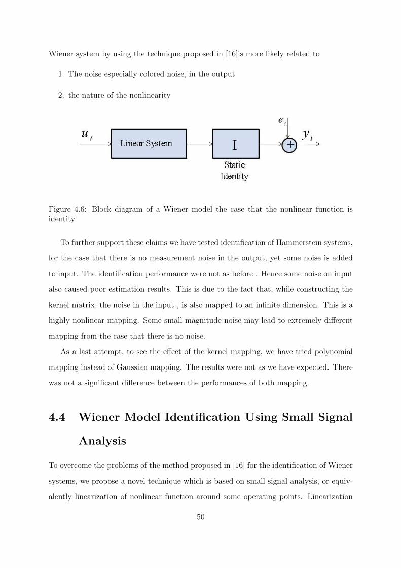
Wiener system by using the technique proposed in [16]is more likely related to
1. The noise especially colored noise, in the output
2. the nature of the nonlinearity
Figure 4.6: Block diagram of a Wiener model the case that the nonlinear function isidentity
To further support these claims we have tested identification of Hammerstein systems,
for the case that there is no measurement noise in the output, yet some noise is added
to input. The identification performance were not as before . Hence some noise on input
also caused poor estimation results. This is due to the fact that, while constructing the
kernel matrix, the noise in the input , is also mapped to an infinite dimension. This is a
highly nonlinear mapping. Some small magnitude noise may lead to extremely different
mapping from the case that there is no noise.
As a last attempt, to see the effect of the kernel mapping, we have tried polynomial
mapping instead of Gaussian mapping. The results were not as we have expected. There
was not a significant difference between the performances of both mapping.
4.4 Wiener Model Identification Using Small Signal
Analysis
To overcome the problems of the method proposed in [16] for the identification of Wiener
systems, we propose a novel technique which is based on small signal analysis, or equiv-
alently linearization of nonlinear function around some operating points. Linearization
50
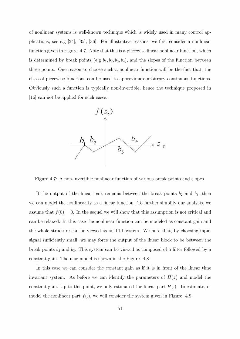
of nonlinear systems is well-known technique which is widely used in many control ap-
plications, see e.g [34], [35], [36]. For illustrative reasons, we first consider a nonlinear
function given in Figure 4.7. Note that this is a piecewise linear nonlinear function, which
is determined by break points (e.g b1, b2, b3, b4), and the slopes of the function between
these points. One reason to choose such a nonlinear function will be the fact that, the
class of piecewise functions can be used to approximate arbitrary continuous functions.
Obviously such a function is typically non-invertible, hence the technique proposed in
[16] can not be applied for such cases.
Figure 4.7: A non-invertible nonlinear function of various break points and slopes
If the output of the linear part remains between the break points b2 and b3, then
we can model the nonlinearity as a linear function. To further simplify our analysis, we
assume that f(0) = 0. In the sequel we will show that this assumption is not critical and
can be relaxed. In this case the nonlinear function can be modeled as constant gain and
the whole structure can be viewed as an LTI system. We note that, by choosing input
signal sufficiently small, we may force the output of the linear block to be between the
break points b2 and b3. This system can be viewed as composed of a filter followed by a
constant gain. The new model is shown in the Figure 4.8
In this case we can consider the constant gain as if it is in front of the linear time
invariant system. As before we can identify the parameters of H(z) and model the
constant gain. Up to this point, we only estimated the linear part H(.). To estimate, or
model the nonlinear part f(.), we will consider the system given in Figure 4.9.
51
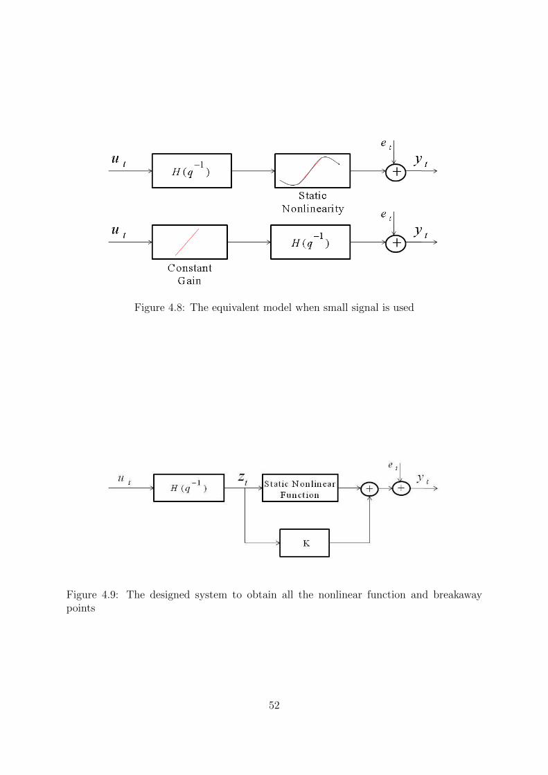
Figure 4.8: The equivalent model when small signal is used
Figure 4.9: The designed system to obtain all the nonlinear function and breakawaypoints
52
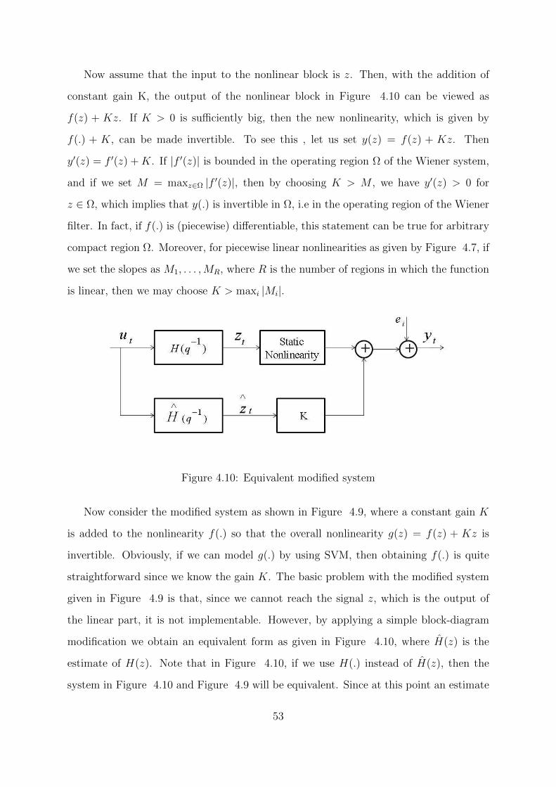
Now assume that the input to the nonlinear block is z. Then, with the addition of
constant gain K, the output of the nonlinear block in Figure 4.10 can be viewed as
f(z) + Kz. If K > 0 is sufficiently big, then the new nonlinearity, which is given by
f(.) + K, can be made invertible. To see this , let us set y(z) = f(z) + Kz. Then
y′(z) = f ′(z) +K. If |f ′(z)| is bounded in the operating region Ω of the Wiener system,
and if we set M = maxz∈Ω |f ′(z)|, then by choosing K > M , we have y′(z) > 0 for
z ∈ Ω, which implies that y(.) is invertible in Ω, i.e in the operating region of the Wiener
filter. In fact, if f(.) is (piecewise) differentiable, this statement can be true for arbitrary
compact region Ω. Moreover, for piecewise linear nonlinearities as given by Figure 4.7, if
we set the slopes as M1, . . . ,MR, where R is the number of regions in which the function
is linear, then we may choose K > maxi |Mi|.
Figure 4.10: Equivalent modified system
Now consider the modified system as shown in Figure 4.9, where a constant gain K
is added to the nonlinearity f(.) so that the overall nonlinearity g(z) = f(z) + Kz is
invertible. Obviously, if we can model g(.) by using SVM, then obtaining f(.) is quite
straightforward since we know the gain K. The basic problem with the modified system
given in Figure 4.9 is that, since we cannot reach the signal z, which is the output of
the linear part, it is not implementable. However, by applying a simple block-diagram
modification we obtain an equivalent form as given in Figure 4.10, where H(z) is the
estimate of H(z). Note that in Figure 4.10, if we use H(.) instead of H(z), then the
system in Figure 4.10 and Figure 4.9 will be equivalent. Since at this point an estimate
53
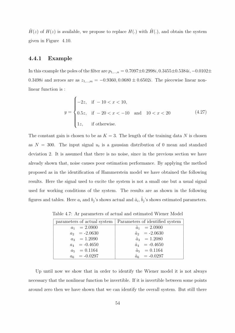
H(z) of H(z) is available, we propose to replace H(.) with H(.), and obtain the system
given in Figure 4.10.
4.4.1 Example
In this example the poles of the filter are p1,...,n = 0.7097±0.2998i, 0.3455±0.5384i,−0.0102±0.3498i and zeroes are as z1,...,m = −0.9360, 0.0680 ± 0.6502i. The piecewise linear non-
linear function is :
y =
−2z, if − 10 < x < 10,
0.5z, if − 20 < x < −10 and 10 < x < 20
1z, if otherwise.
(4.27)
The constant gain is chosen to be as K = 3. The length of the training data N is chosen
as N = 300. The input signal ut is a gaussian distribution of 0 mean and standard
deviation 2. It is assumed that there is no noise, since in the previous section we have
already shown that, noise causes poor estimation performance. By applying the method
proposed as in the identification of Hammerstein model we have obtained the following
results. Here the signal used to excite the system is not a small one but a usual signal
used for working conditions of the system. The results are as shown in the following
figures and tables. Here ai and bj’s shows actual and ai, bj’s shows estimated parameters.
Table 4.7: Ar parameters of actual and estimated Wiener Model
parameters of actual system Parameters of identified systema1 = 2.0900 a1 = 2.0900a2 = -2.0630 a2 = -2.0630a3 = 1.2090 a3 = 1.2080a4 = -0.4650 a4 = -0.4650a5 = 0.1164 a5 = 0.1164a6 = -0.0297 a6 = -0.0297
Up until now we show that in order to identify the Wiener model it is not always
necessary that the nonlinear function be invertible. If it is invertible between some points
around zero then we have shown that we can identify the overall system. But still there
54
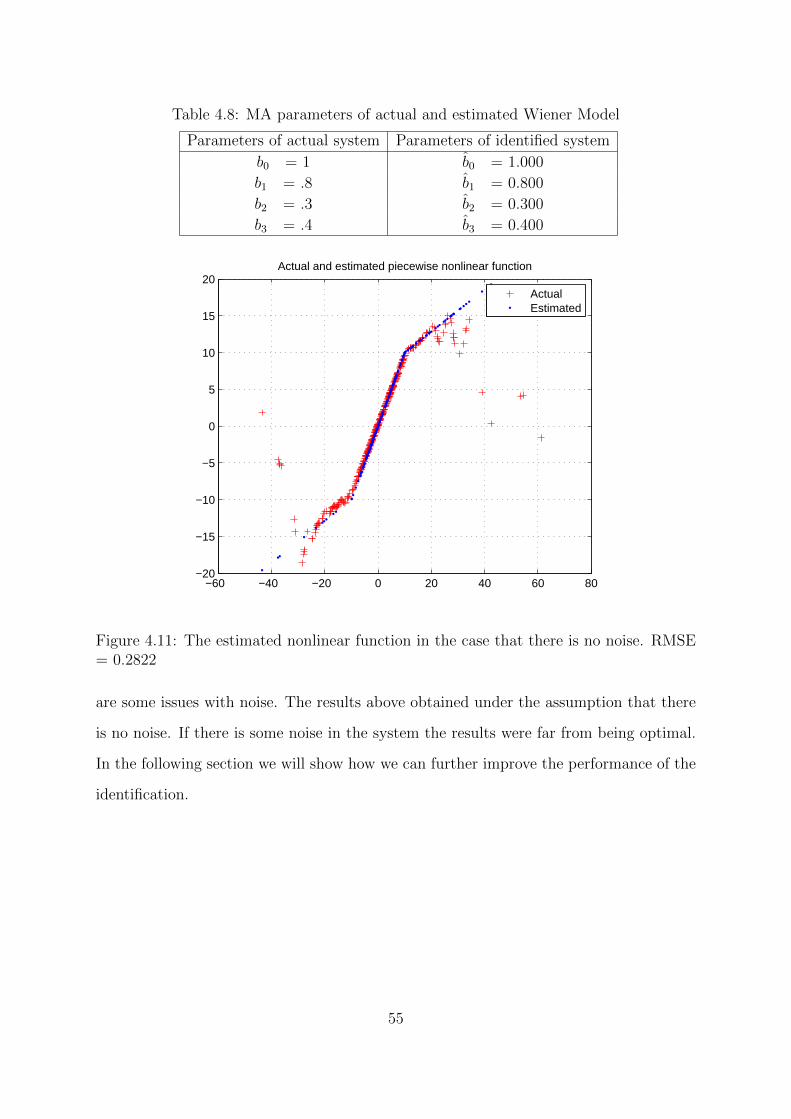
Table 4.8: MA parameters of actual and estimated Wiener Model
Parameters of actual system Parameters of identified system
b0 = 1 b0 = 1.000
b1 = .8 b1 = 0.800
b2 = .3 b2 = 0.300
b3 = .4 b3 = 0.400
−60 −40 −20 0 20 40 60 80−20
−15
−10
−5
0
5
10
15
20Actual and estimated piecewise nonlinear function
ActualEstimated
Figure 4.11: The estimated nonlinear function in the case that there is no noise. RMSE= 0.2822
are some issues with noise. The results above obtained under the assumption that there
is no noise. If there is some noise in the system the results were far from being optimal.
In the following section we will show how we can further improve the performance of the
identification.
55
4.5 Another Approach for Wiener Model Identifica-
tion
In this section, we will propose another method for the identification of Wiener systems
based on the ideas presented in previous section. Similar to the technique presented in
previous section, the new method is also based on linearization, hence we utilize small-
signal analysis. Subsequently by applying an approach similar to the identification of
Hammerstein models we can also identify the Wiener model. Consequently, similar to the
previous method, we obtain the transfer function of the linear part and a gain K. Then
by designing various system models and using SVM appropriately we can determine the
static nonlinear function by using least-squares support vector regression. Consequently,
the overall Wiener system can be identified.
4.5.1 Determination of the magnitude of the input signal
If we choose sufficiently small input signals, then the signal z which is the input to the
nonlinear block will be sufficiently small, and consequently we can linearize the nonlinear
block around the operating point. In this instance the question ’how small the input
signal should be?’ raises. The answer for this question varies considerably from system
to system and also depends on the method that is used to identify the system. Since
we use SVM in this work the rank of the kernel matrix should not be small, [1]. SVM
parameters should be chosen such that this condition is satisfied.
We propose a solution for the problems stated above. The proposed method that we
apply is an algorithm composed of some steps. The method determines experimentally
how small the magnitude of the input signal should be . The steps are given below.
step 1: Choose a signal of small magnitude randomly.
step 2: Excite the system with this signal and obtain the output.
step 3: Multiply the magnitude of the input signal in the 1st step with a gain of positive
k that is greater than 1.
56
step 4: Excite the system with the signal that is obtained at the step 3 and obtain
the output of the system. If the magnitude of the obtained output at step 4 is
sufficiently close to k times the magnitude of the output obtained at step 2 then
we say that the system is working in its linear range. In that case multiply the
magnitude of the signal at the step 3 with a gain k which is not necessarily the
same as the gain k used before and apply this new signal to the system as input,
obtain the outputs and compare them. Keep applying these steps as long as the
output is also k times the output of the previous step. If not, record the signal
obtained at the last step and choose the magnitude of the input signal such that it
remains in the margin of the magnitude of the signal obtained at the last step.
These steps are shown as an algorithm flowchart as in the Figure 4.12.
Note that this algorithm may not give an exact solution, [37]. But our simulations
indicate that it improves the estimations considerably. We could have chosen an extremely
small input signal to excite the system which would justify the linearization. But since
there will always be some noise while obtaining the output data, and since the input is
small the output will also be small and thus the noise will have more effect than the filter.
In that case we will be simply trying to fit the noise, in which case obviously estimation
error will increase and the results will not be meaningful.
4.5.2 Identification of Wiener Model
After determining the input signal we can utilize SVM.
SVM will model a static linear gain (K) instead of a static nonlinear function. Besides
we will be able to obtain the numerator and denominator parameters of the filter. The
identification task will not end even after obtaining these parameters. To identify the
nonlinear part, we use a system as shown in the Figure 4.14.
Note that in Figure 4.14 H(.) represents the estimated transfer function of the linear
part. Obviously, we can not measure zt, which is the input to the nonlinear block, but
we can compute its estimation zt. Then by applying ut, we can measure yt and compute
57
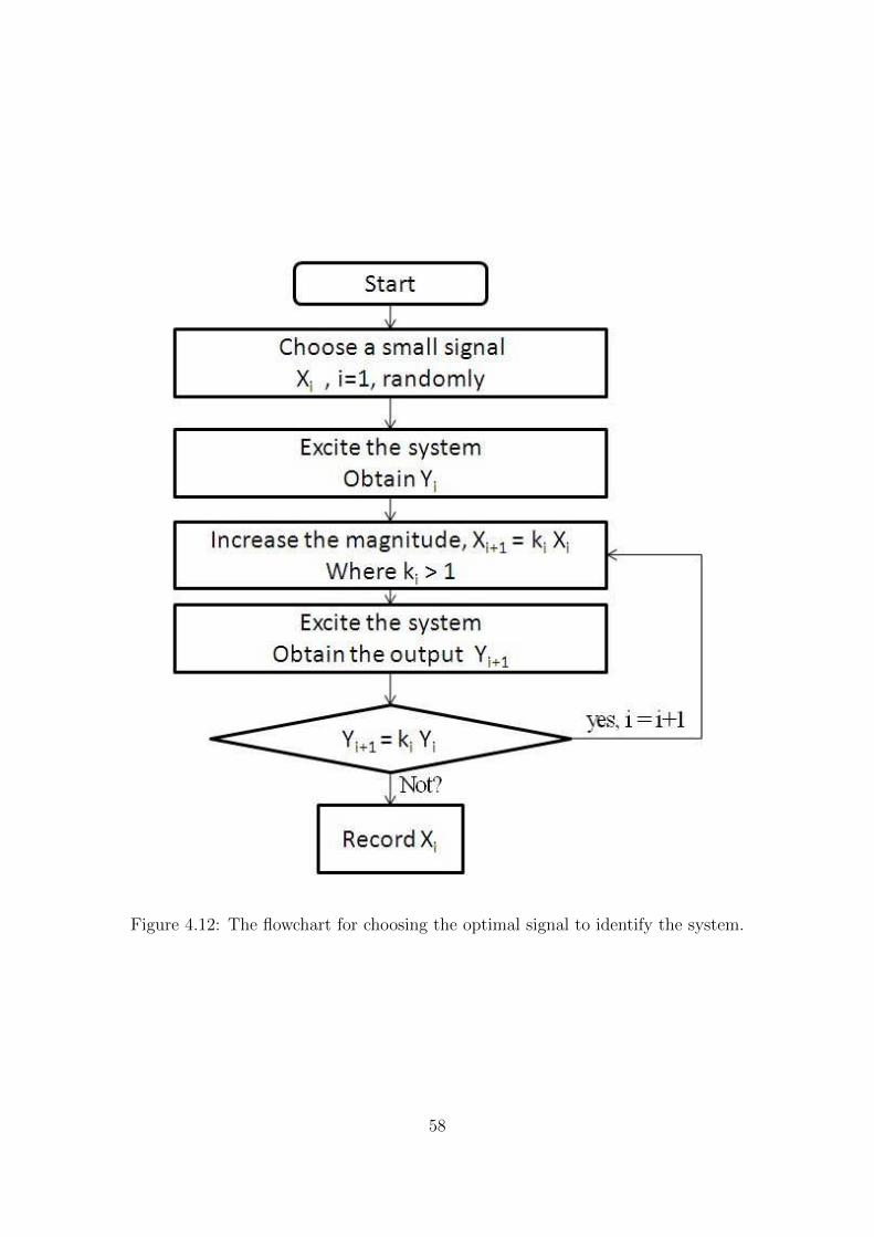
Figure 4.12: The flowchart for choosing the optimal signal to identify the system.
58

Figure 4.13: The actual Wiener model is as at the top figure. We can put the gain infront of the filter when small signals are used as in the bottom figure.
Figure 4.14: The designed system for identifying the whole of static nonlinear function.
59
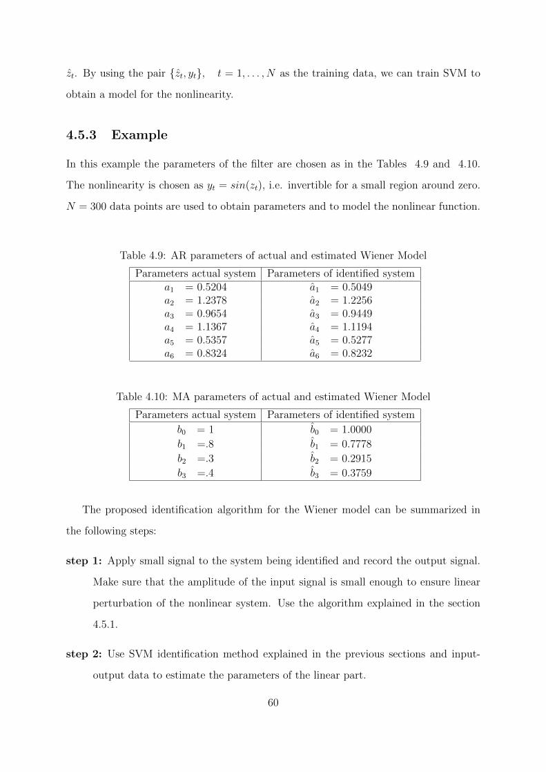
zt. By using the pair zt, yt, t = 1, . . . , N as the training data, we can train SVM to
obtain a model for the nonlinearity.
4.5.3 Example
In this example the parameters of the filter are chosen as in the Tables 4.9 and 4.10.
The nonlinearity is chosen as yt = sin(zt), i.e. invertible for a small region around zero.
N = 300 data points are used to obtain parameters and to model the nonlinear function.
Table 4.9: AR parameters of actual and estimated Wiener Model
Parameters actual system Parameters of identified systema1 = 0.5204 a1 = 0.5049a2 = 1.2378 a2 = 1.2256a3 = 0.9654 a3 = 0.9449a4 = 1.1367 a4 = 1.1194a5 = 0.5357 a5 = 0.5277a6 = 0.8324 a6 = 0.8232
Table 4.10: MA parameters of actual and estimated Wiener Model
Parameters actual system Parameters of identified system
b0 = 1 b0 = 1.0000
b1 =.8 b1 = 0.7778
b2 =.3 b2 = 0.2915
b3 =.4 b3 = 0.3759
The proposed identification algorithm for the Wiener model can be summarized in
the following steps:
step 1: Apply small signal to the system being identified and record the output signal.
Make sure that the amplitude of the input signal is small enough to ensure linear
perturbation of the nonlinear system. Use the algorithm explained in the section
4.5.1.
step 2: Use SVM identification method explained in the previous sections and input-
output data to estimate the parameters of the linear part.
60
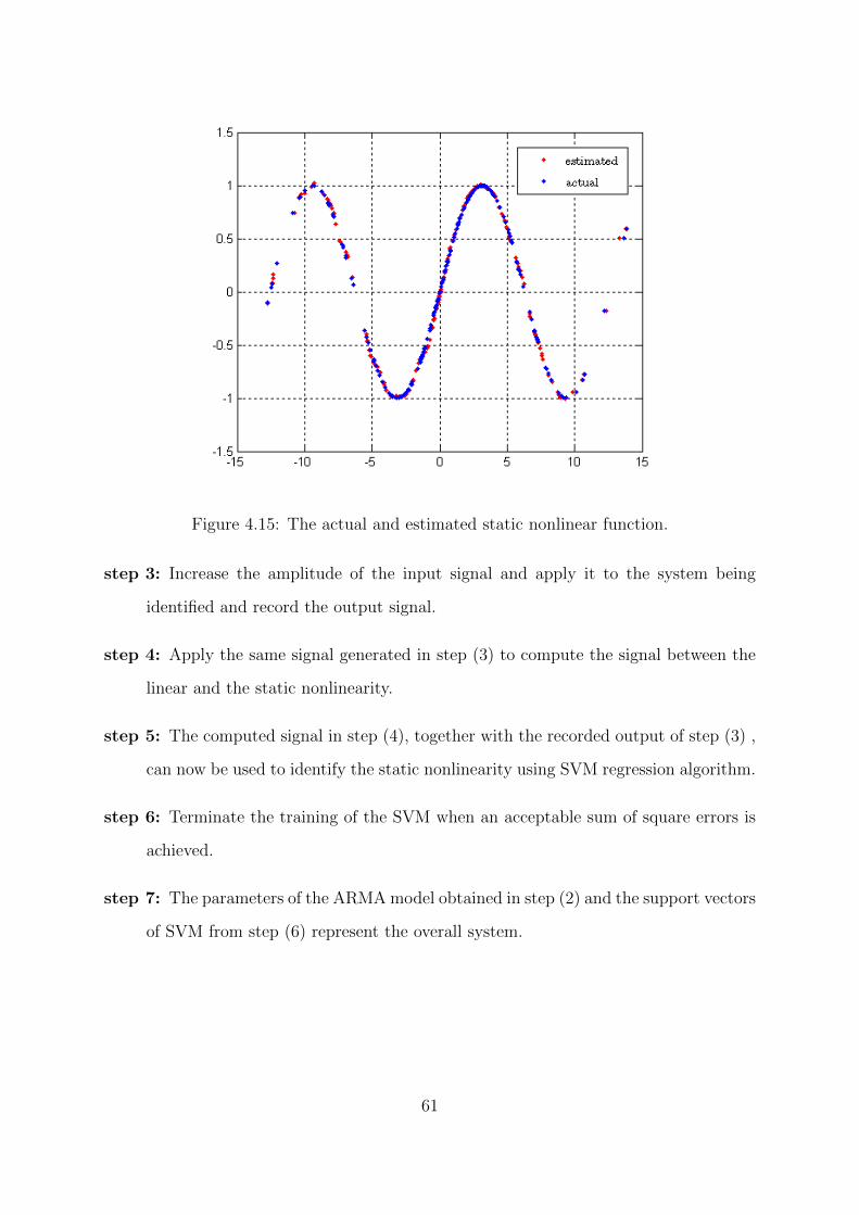
Figure 4.15: The actual and estimated static nonlinear function.
step 3: Increase the amplitude of the input signal and apply it to the system being
identified and record the output signal.
step 4: Apply the same signal generated in step (3) to compute the signal between the
linear and the static nonlinearity.
step 5: The computed signal in step (4), together with the recorded output of step (3) ,
can now be used to identify the static nonlinearity using SVM regression algorithm.
step 6: Terminate the training of the SVM when an acceptable sum of square errors is
achieved.
step 7: The parameters of the ARMAmodel obtained in step (2) and the support vectors
of SVM from step (6) represent the overall system.
61
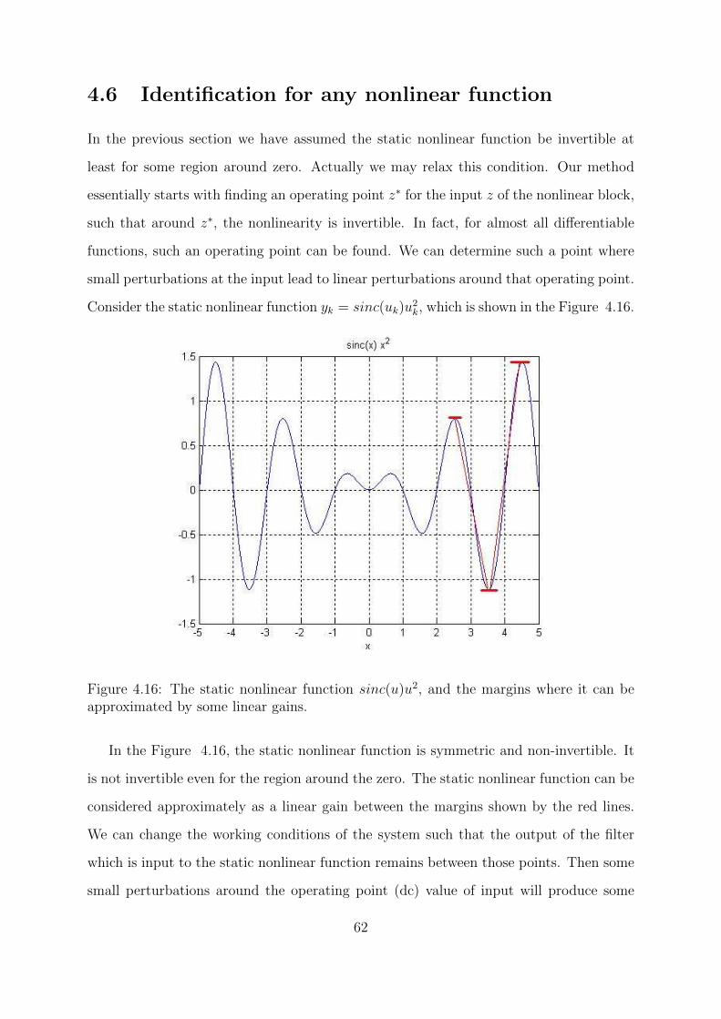
4.6 Identification for any nonlinear function
In the previous section we have assumed the static nonlinear function be invertible at
least for some region around zero. Actually we may relax this condition. Our method
essentially starts with finding an operating point z∗ for the input z of the nonlinear block,
such that around z∗, the nonlinearity is invertible. In fact, for almost all differentiable
functions, such an operating point can be found. We can determine such a point where
small perturbations at the input lead to linear perturbations around that operating point.
Consider the static nonlinear function yk = sinc(uk)u2k, which is shown in the Figure 4.16.
Figure 4.16: The static nonlinear function sinc(u)u2, and the margins where it can beapproximated by some linear gains.
In the Figure 4.16, the static nonlinear function is symmetric and non-invertible. It
is not invertible even for the region around the zero. The static nonlinear function can be
considered approximately as a linear gain between the margins shown by the red lines.
We can change the working conditions of the system such that the output of the filter
which is input to the static nonlinear function remains between those points. Then some
small perturbations around the operating point (dc) value of input will produce some
62
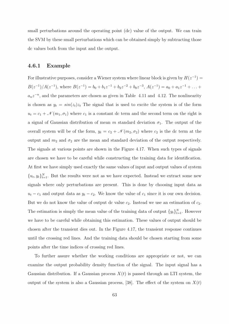
small perturbations around the operating point (dc) value of the output. We can train
the SVM by these small perturbations which can be obtained simply by subtracting those
dc values both from the input and the output.
4.6.1 Example
For illustrative purposes, consider aWiener system where linear block is given byH(z−1) =
B(z−1)/A(z−1), where B(z−1) = b0 + b1z−1 + b2z
−2 + b0z−3, A(z−1) = a0 + a1z
−1 + . . .+
anz−n, and the parameters are chosen as given in Table 4.11 and 4.12. The nonlinearity
is chosen as yt = sin(zt)zt The signal that is used to excite the system is of the form
ut = c1 + N (m1, σ1) where c1 is a constant dc term and the second term on the right is
a signal of Gaussian distribution of mean m standard deviation σ1. The output of the
overall system will be of the form, yt = c2 + N (m2, σ2) where c2 is the dc term at the
output and m2 and σ2 are the mean and standard deviation of the output respectively.
The signals at various points are shown in the Figure 4.17. When such types of signals
are chosen we have to be careful while constructing the training data for identification.
At first we have simply used exactly the same values of input and output values of system
ut, ytNt=1. But the results were not as we have expected. Instead we extract some new
signals where only perturbations are present. This is done by choosing input data as
ut − c1 and output data as yt − c2. We know the value of c1 since it is our own decision.
But we do not know the value of output dc value c2. Instead we use an estimation of c2.
The estimation is simply the mean value of the training data of output ytNt=1. However
we have to be careful while obtaining this estimation. These values of output should be
chosen after the transient dies out. In the Figure 4.17, the transient response continues
until the crossing red lines. And the training data should be chosen starting from some
points after the time indices of crossing red lines.
To further assure whether the working conditions are appropriate or not, we can
examine the output probability density function of the signal. The input signal has a
Gaussian distribution. If a Gaussian process X(t) is passed through an LTI system, the
output of the system is also a Gaussian process, [38]. The effect of the system on X(t)
63
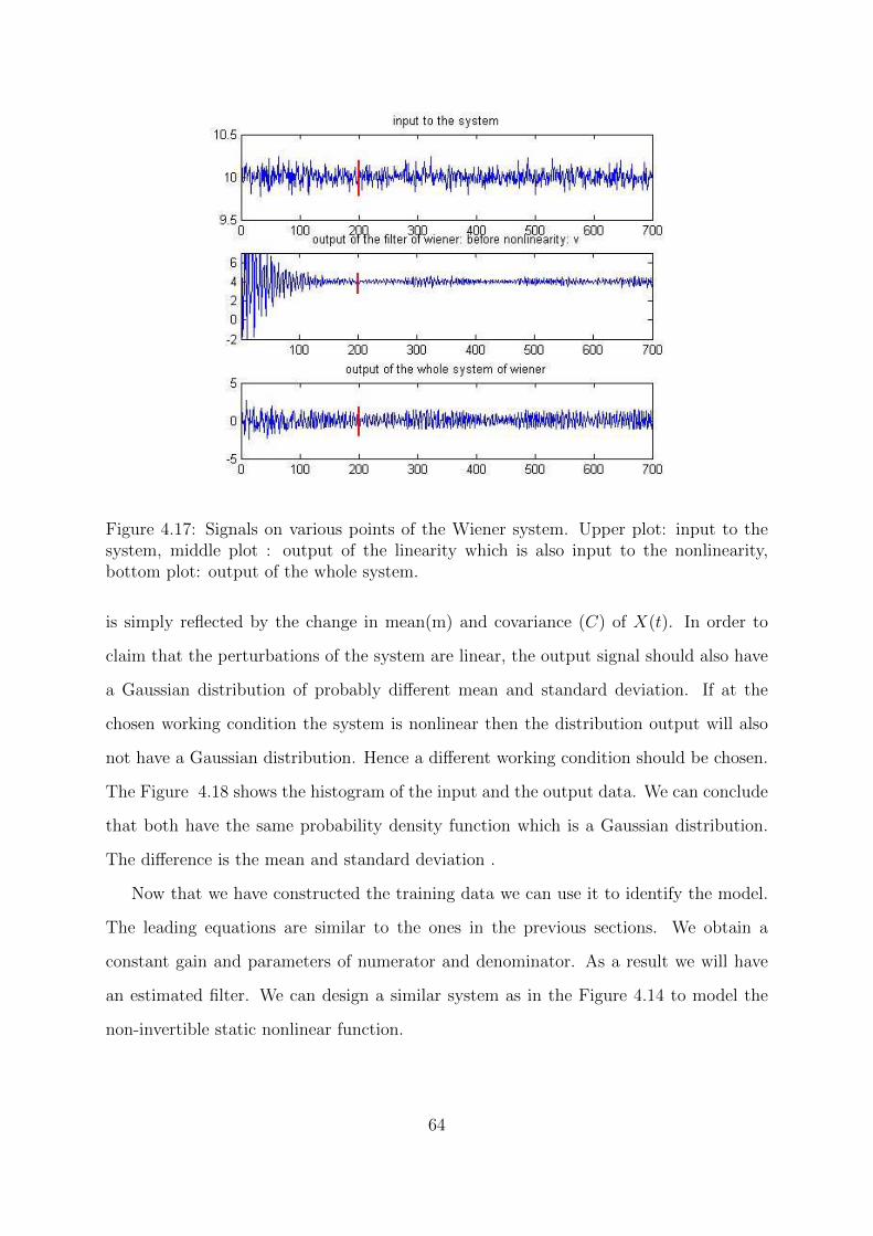
Figure 4.17: Signals on various points of the Wiener system. Upper plot: input to thesystem, middle plot : output of the linearity which is also input to the nonlinearity,bottom plot: output of the whole system.
is simply reflected by the change in mean(m) and covariance (C) of X(t). In order to
claim that the perturbations of the system are linear, the output signal should also have
a Gaussian distribution of probably different mean and standard deviation. If at the
chosen working condition the system is nonlinear then the distribution output will also
not have a Gaussian distribution. Hence a different working condition should be chosen.
The Figure 4.18 shows the histogram of the input and the output data. We can conclude
that both have the same probability density function which is a Gaussian distribution.
The difference is the mean and standard deviation .
Now that we have constructed the training data we can use it to identify the model.
The leading equations are similar to the ones in the previous sections. We obtain a
constant gain and parameters of numerator and denominator. As a result we will have
an estimated filter. We can design a similar system as in the Figure 4.14 to model the
non-invertible static nonlinear function.
64
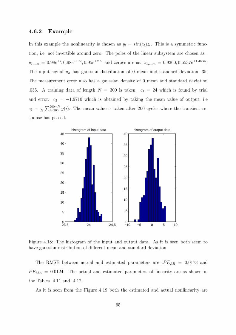
4.6.2 Example
In this example the nonlinearity is chosen as yt = sin(zt)zt. This is a symmetric func-
tion, i.e, not invertible around zero. The poles of the linear subsystem are chosen as .
p1,...,n = 0.98e±i, 0.98e±1.6i, 0.95e±2.5i and zeroes are as: z1,...,m = 0.9360, 0.6537e±1.4666i.
The input signal uk has gaussian distribution of 0 mean and standard deviation .35.
The measurement error also has a gaussian density of 0 mean and standard deviation
.035. A training data of length N = 300 is taken. c1 = 24 which is found by trial
and error. c2 = −1.9710 which is obtained by taking the mean value of output, i.e
c2 = 1N
∑200+Ni=200 y(i). The mean value is taken after 200 cycles where the transient re-
sponse has passed.
23.5 24 24.50
5
10
15
20
25
30
35
40
45histogram of input data
−10 −5 0 5 100
5
10
15
20
25
30
35
40histogram of output data
Figure 4.18: The histogram of the input and output data. As it is seen both seem tohave gaussian distribution of different mean and standard deviation
The RMSE between actual and estimated parameters are :PEAR = 0.0173 and
PEMA = 0.0124. The actual and estimated parameters of linearity are as shown in
the Tables 4.11 and 4.12.
As it is seen from the Figure 4.19 both the estimated and actual nonlinearity are
65
−10 −5 0 5 10−6
−4
−2
0
2
4
6
8actual and estimated nolinearities
estimated nonlinearityactual nonlinearity
Figure 4.19: Non-invertible sin(x)x is modeled with an accurate precision. RMSE =0.1682
almost indistinguishable.
Table 4.11: AR parameters of actual and estimated Wiener Model
Parameters of actual system Parameters of identified systema1 = 0.5204 a1 = 0.5103a2 = 1.2378 a2 = 1.2310a3 = 0.9654 a3 = 0.9551a4 = 1.1367 a4 = 1.1256a5 = 0.5357 a5 = 0.5323a6 = 0.8324 a6 = 0.8234
4.7 Control of Wiener Systems After Identification
The overall aim of identification is to model an unknown system and more importantly
to control it, see e.g. [39] , [40]. After we have estimated the filter and modeled the static
nonlinear function we can design a closed loop system and control the overall system.
The designed system is as in the Figure 4.20.
66

Table 4.12: MA parameters of actual and estimated Wiener Model
Parameters of actual system Parameters of identified system
b0 = 1 b0 = 1.0000
b1 =.8 b1 = 0.7970
b2 =.3 b2 = 0.2880
b3 =.4 b3 = 0.3990
Figure 4.20: The designed closed loop Wiener system for control.
In the Figure 4.20, the output is fed to SVM which models the inverse of the static
nonlinearity. Obviously, at this point, we assume that the nonlinearity f(.) is invertible.
It is trained such that given the output yt the input to the static nonlinearity zt which is
the output of the filter is obtained. The overall model can be considered as if the output
of the filter is taken as shown by the dashed line. Hence we can use the well known linear
control theory. The closed loop system may be unstable even if the filter itself is stable.
As shown in the Figure 4.22. the step response diverges to infinity.
Figure 4.21: A controller is added to make the overall system stable and meet designspecifications.
67
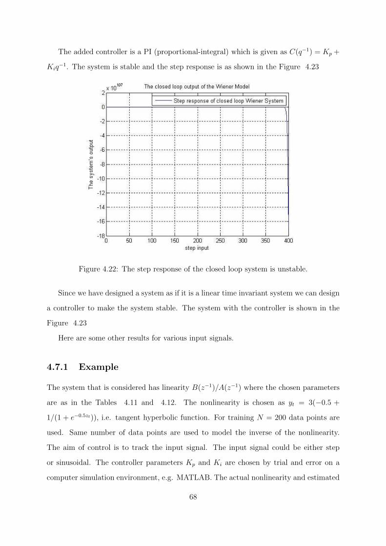
The added controller is a PI (proportional-integral) which is given as C(q−1) = Kp +
Kiq−1. The system is stable and the step response is as shown in the Figure 4.23
Figure 4.22: The step response of the closed loop system is unstable.
Since we have designed a system as if it is a linear time invariant system we can design
a controller to make the system stable. The system with the controller is shown in the
Figure 4.23
Here are some other results for various input signals.
4.7.1 Example
The system that is considered has linearity B(z−1)/A(z−1) where the chosen parameters
are as in the Tables 4.11 and 4.12. The nonlinearity is chosen as yt = 3(−0.5 +
1/(1 + e−0.5zt)), i.e. tangent hyperbolic function. For training N = 200 data points are
used. Same number of data points are used to model the inverse of the nonlinearity.
The aim of control is to track the input signal. The input signal could be either step
or sinusoidal. The controller parameters Kp and Ki are chosen by trial and error on a
computer simulation environment, e.g. MATLAB. The actual nonlinearity and estimated
68

0 50 100 150 200 250 300 350 400 4500.4
0.5
0.6
0.7
0.8
0.9
1
1.1
1.2
1.3The closed loop output of the Wiener Model: A controller is added
input
The
sys
tem
’s o
utpu
t
Step input to closed loop Wiener System, with controlleroutput of the filter
Figure 4.23: After the controller is added the system became stable.
nonlinearity together with their inverses are shown in the Figure
69
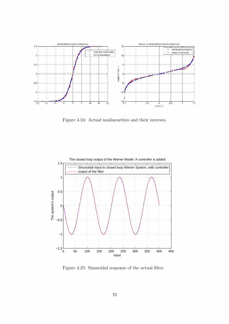
Figure 4.24: Actual nonlinearities and their inverses.
0 50 100 150 200 250 300 350 400 450−1.5
−1
−0.5
0
0.5
1
1.5The closed loop output of the Wiener Model: A controller is added
input
The
sys
tem
’s o
utpu
t
Sinusoidal input to closed loop Wiener System, with controlleroutput of the filter
Figure 4.25: Sinusoidal response of the actual filter.
70
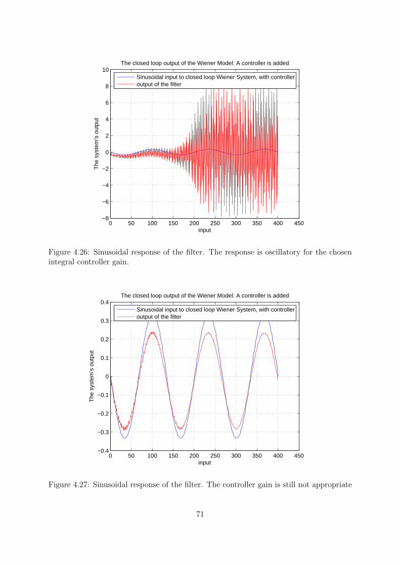
0 50 100 150 200 250 300 350 400 450−8
−6
−4
−2
0
2
4
6
8
10The closed loop output of the Wiener Model: A controller is added
input
The
sys
tem
’s o
utpu
t
Sinusoidal input to closed loop Wiener System, with controlleroutput of the filter
Figure 4.26: Sinusoidal response of the filter. The response is oscillatory for the chosenintegral controller gain.
0 50 100 150 200 250 300 350 400 450−0.4
−0.3
−0.2
−0.1
0
0.1
0.2
0.3
0.4The closed loop output of the Wiener Model: A controller is added
input
The
sys
tem
’s o
utpu
t
Sinusoidal input to closed loop Wiener System, with controlleroutput of the filter
Figure 4.27: Sinusoidal response of the filter. The controller gain is still not appropriate
71
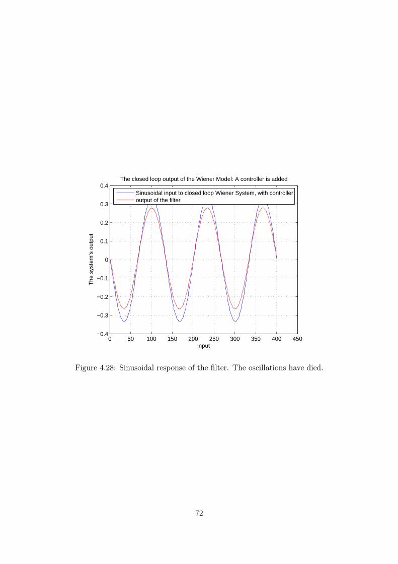
0 50 100 150 200 250 300 350 400 450−0.4
−0.3
−0.2
−0.1
0
0.1
0.2
0.3
0.4The closed loop output of the Wiener Model: A controller is added
input
The
sys
tem
’s o
utpu
t
Sinusoidal input to closed loop Wiener System, with controlleroutput of the filter
Figure 4.28: Sinusoidal response of the filter. The oscillations have died.
72
Chapter 5
IDENTIFICATION OF
WIENER-HAMMERSTEIN
SYSTEMS BY LS-SVM
In this chapter we will use LS-SVM to identify Wiener-Hammerstein systems. We note
that this problem is set as a future work in [1]. First we will assume that we know the
static nonlinear function and identify the system. Then we will develop a new procedure
to identify Wiener-Hammerstein systems in which case we will assume that nonlinear
function is unknown. Then we will identify it as a black box model and compare it with
some other approaches.
A Wiener-Hammerstein system, as the name implies, is composed of a Wiener system
followed by a Hammerstein system. It is a more complicated nonlinear model compared
to the Wiener and Hammerstein models. The model is as shown in the Figure 5.1.
There are two LTI systems separated by a static nonlinear function. Let us assume
that the transfer functions H1(.) and H2(.) are given as follows
H1(q−1) =
b0 + b1q−1 + . . .+ bmq
−m
1 + a1q−1 + . . .+ anq−n(5.1)
H2(q−1) =
d0 + d1q−1 + . . .+ dlq
−l
1 + c1q−1 + . . .+ ckq−k(5.2)
The orders of these transfer functions may be arbitrary. But we will assume that we
73
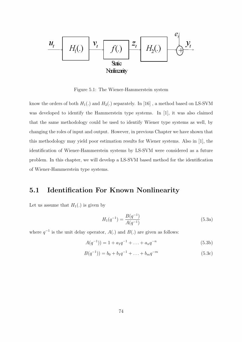
Figure 5.1: The Wiener-Hammerstein system
know the orders of both H1(.) and H2(.) separately. In [16] , a method based on LS-SVM
was developed to identify the Hammerstein type systems. In [1], it was also claimed
that the same methodology could be used to identify Wiener type systems as well, by
changing the roles of input and output. However, in previous Chapter we have shown that
this methodology may yield poor estimation results for Wiener systems. Also in [1], the
identification of Wiener-Hammerstein systems by LS-SVM were considered as a future
problem. In this chapter, we will develop a LS-SVM based method for the identification
of Wiener-Hammerstein type systems.
5.1 Identification For Known Nonlinearity
Let us assume that H1(.) is given by
H1(q−1) =
B(q−1)
A(q−1)(5.3a)
where q−1 is the unit delay operator, A(.) and B(.) are given as follows:
A(q−1)) = 1 + a1q−1 + . . .+ anq
−n (5.3b)
B(q−1)) = b0 + b1q−1 + . . .+ bmq
−m (5.3c)
74
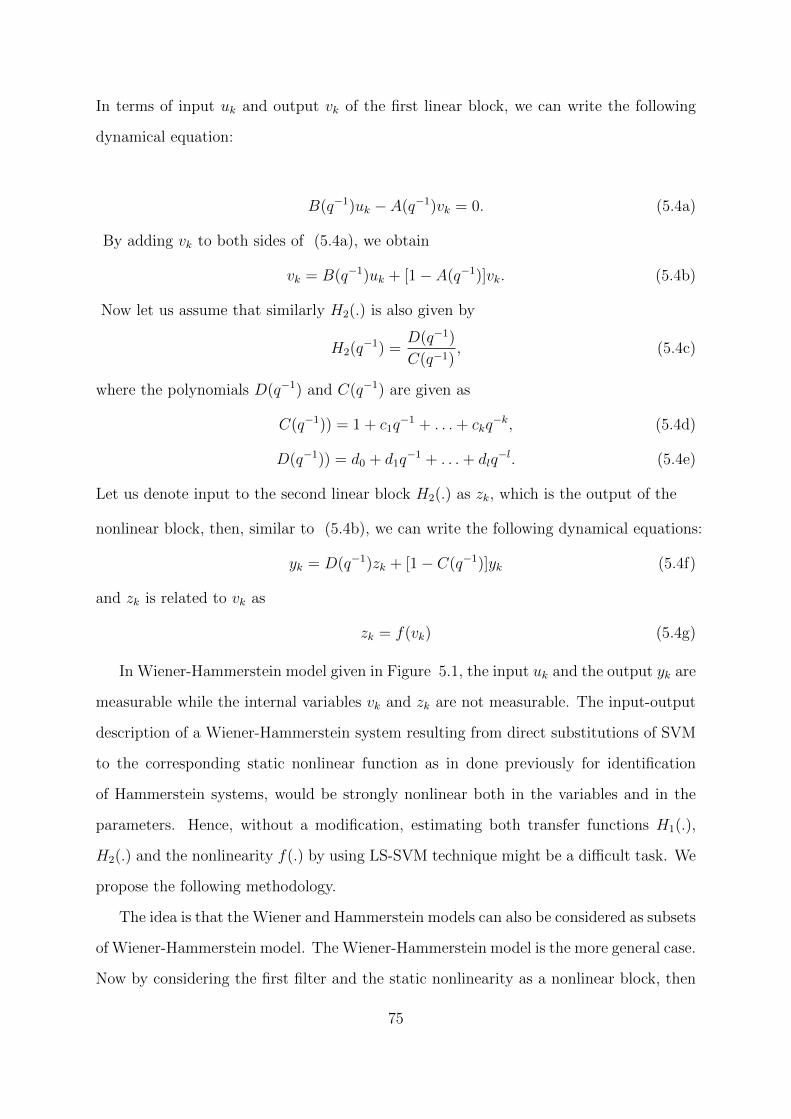
In terms of input uk and output vk of the first linear block, we can write the following
dynamical equation:
B(q−1)uk − A(q−1)vk = 0. (5.4a)
By adding vk to both sides of (5.4a), we obtain
vk = B(q−1)uk + [1− A(q−1)]vk. (5.4b)
Now let us assume that similarly H2(.) is also given by
H2(q−1) =
D(q−1)
C(q−1), (5.4c)
where the polynomials D(q−1) and C(q−1) are given as
C(q−1)) = 1 + c1q−1 + . . .+ ckq
−k, (5.4d)
D(q−1)) = d0 + d1q−1 + . . .+ dlq
−l. (5.4e)
Let us denote input to the second linear block H2(.) as zk, which is the output of the
nonlinear block, then, similar to (5.4b), we can write the following dynamical equations:
yk = D(q−1)zk + [1− C(q−1)]yk (5.4f)
and zk is related to vk as
zk = f(vk) (5.4g)
In Wiener-Hammerstein model given in Figure 5.1, the input uk and the output yk are
measurable while the internal variables vk and zk are not measurable. The input-output
description of a Wiener-Hammerstein system resulting from direct substitutions of SVM
to the corresponding static nonlinear function as in done previously for identification
of Hammerstein systems, would be strongly nonlinear both in the variables and in the
parameters. Hence, without a modification, estimating both transfer functions H1(.),
H2(.) and the nonlinearity f(.) by using LS-SVM technique might be a difficult task. We
propose the following methodology.
The idea is that the Wiener and Hammerstein models can also be considered as subsets
of Wiener-Hammerstein model. The Wiener-Hammerstein model is the more general case.
Now by considering the first filter and the static nonlinearity as a nonlinear block, then
75
the overall system can be seen as a Hammerstein model which has a non-static nonlinear
function. The new diagram is shown as in the Figure 5.2.
Figure 5.2: The Wiener-Hammerstein system as a Hammerstein model
Since the nonlinear block is non-static, instead of taking uk, yk as the training data,
we propose to take vectorial training data as xk, yk where regression vector x(k) is
given as:
x(k) =
u(k)
...
u(k − nu)
(5.5)
where nu denotes the lag for input, i.e nu = l+m We have applied similar procedures in
the identification of Hammerstein model but the results were not successful. The reason
could be the fact that since the first filter is ARMA, we consider only the input values
while training. An ARMA filter causes an infinite memory. It could be better if we
also take into consideration the output of the first filter. But due to the structure of
Hammerstein systems, we can only measure the output yk, but not the output of the first
filter, i.e vk in Figure 5.1.
As we introduced in Chapter 4, we can apply a small signal analysis to see if we
can still identify the parameters of the filter and model the static nonlinearity. Many
assumptions are similar to the case of identification of Wiener models. If the input signal
is small enough then the static nonlinearity can be considered as constant gain while the
overall system will be seen as a linear system. The equivalent model when small signals
are used is as in the Figure 5.3.
76
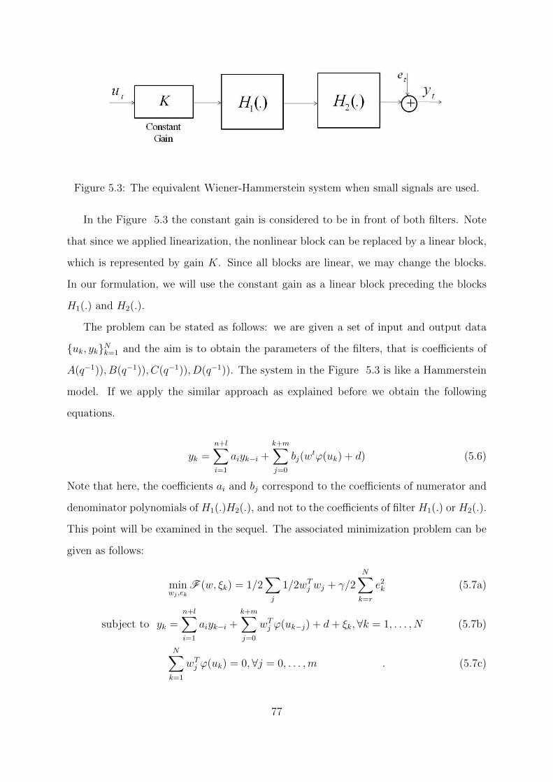
Figure 5.3: The equivalent Wiener-Hammerstein system when small signals are used.
In the Figure 5.3 the constant gain is considered to be in front of both filters. Note
that since we applied linearization, the nonlinear block can be replaced by a linear block,
which is represented by gain K. Since all blocks are linear, we may change the blocks.
In our formulation, we will use the constant gain as a linear block preceding the blocks
H1(.) and H2(.).
The problem can be stated as follows: we are given a set of input and output data
uk, ykNk=1 and the aim is to obtain the parameters of the filters, that is coefficients of
A(q−1)), B(q−1)), C(q−1)), D(q−1)). The system in the Figure 5.3 is like a Hammerstein
model. If we apply the similar approach as explained before we obtain the following
equations.
yk =n+l∑i=1
aiyk−i +k+m∑j=0
bj(wtϕ(uk) + d) (5.6)
Note that here, the coefficients ai and bj correspond to the coefficients of numerator and
denominator polynomials of H1(.)H2(.), and not to the coefficients of filter H1(.) or H2(.).
This point will be examined in the sequel. The associated minimization problem can be
given as follows:
minwj ,ek
F (w, ξk) = 1/2∑j
1/2wTj wj + γ/2
N∑
k=r
e2k (5.7a)
subject to yk =n+l∑i=1
aiyk−i +k+m∑j=0
wTj ϕ(uk−j) + d+ ξk,∀k = 1, . . . , N (5.7b)
N∑
k=1
wTj ϕ(uk) = 0, ∀j = 0, . . . ,m . (5.7c)
77
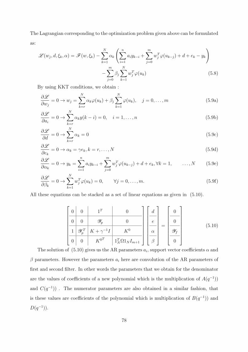
The Lagrangian corresponding to the optimization problem given above can be formulated
as:
L (wj, d, ξk, α) = F (w, ξk)−N∑
k=1
αk
(n∑
i=1
aiyk−i +m∑j=0
wTj ϕ(uk−j) + d+ ek − yk
)
−m∑j=0
βj
N∑
k=1
wTj ϕ(uk) (5.8)
By using KKT conditions, we obtain :
∂L
∂wj
= 0 → wj =N∑
k=r
αkϕ(uk) + βj
N∑
k=1
ϕ(uk), j = 0, . . . ,m (5.9a)
∂L
∂ai= 0 →
N∑
k=r
αky(k − i) = 0, i = 1, . . . , n (5.9b)
∂L
∂d= 0 →
N∑
k=r
αk = 0 (5.9c)
∂L
∂ek= 0 → αk = γek, k = r, . . . , N (5.9d)
∂L
∂αk
= 0 → yk =n∑
i=1
aiyk−i +m∑j=0
wTj ϕ(uk−j) + d+ ek,∀k = 1, . . . , N (5.9e)
∂L
∂βk
= 0 →N∑
k=1
wTj ϕ(uk) = 0, ∀j = 0, . . . ,m. (5.9f)
All these equations can be stacked as a set of linear equations as given in (5.10).
0 0 1T 0
0 0 Yp 0
1 Y Tp K + γ−1I K0
0 0 K0T 1TNΩ1NIm+1
d
e
α
β
=
0
0
Yf
0
(5.10)
The solution of (5.10) gives us the AR parameters ai, support vector coefficients α and
β parameters. However the parameters ai here are convolution of the AR parameters of
first and second filter. In other words the parameters that we obtain for the denominator
are the values of coefficients of a new polynomial which is the multiplication of A(q−1))
and C(q−1)) . The numerator parameters are also obtained in a similar fashion, that
is these values are coefficients of the polynomial which is multiplication of B(q−1)) and
D(q−1)).
78
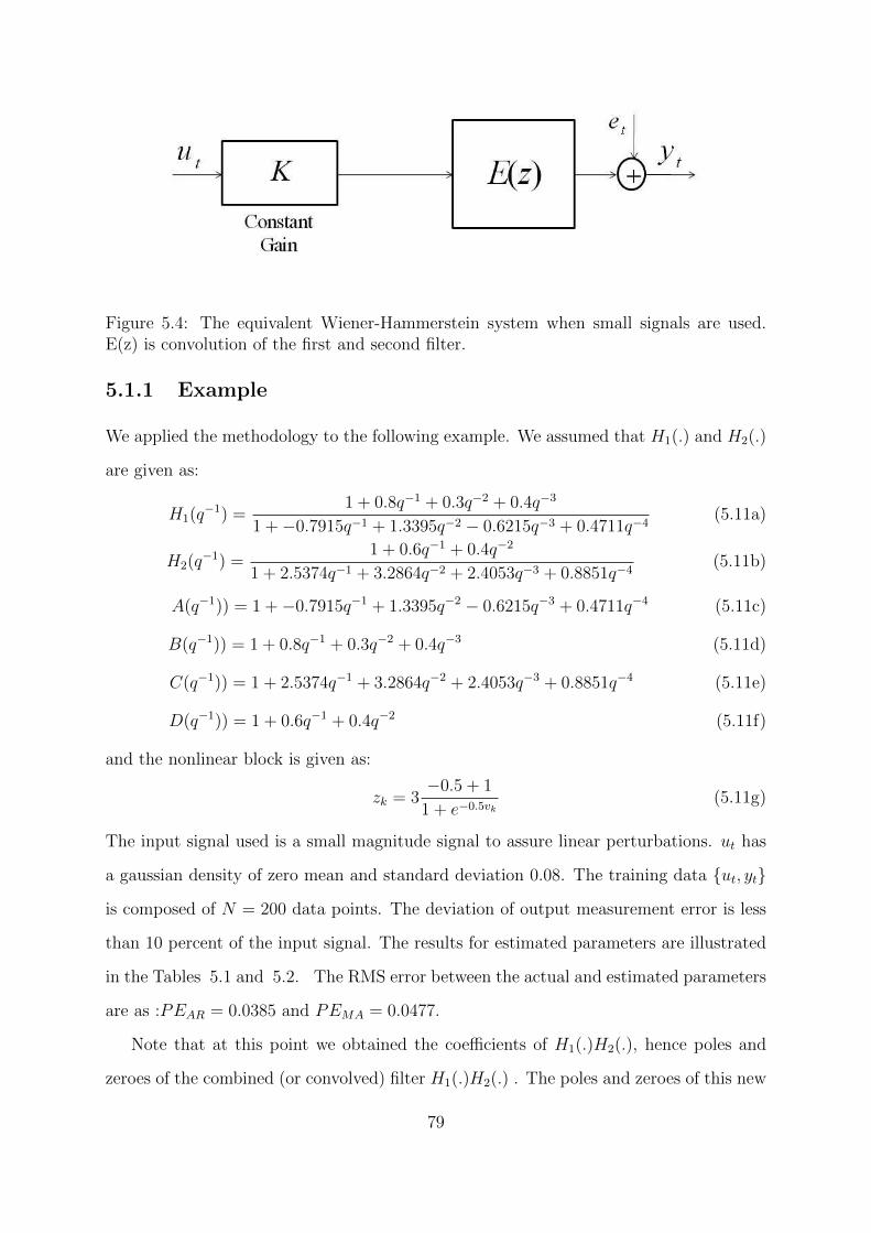
Figure 5.4: The equivalent Wiener-Hammerstein system when small signals are used.E(z) is convolution of the first and second filter.
5.1.1 Example
We applied the methodology to the following example. We assumed that H1(.) and H2(.)
are given as:
H1(q−1) =
1 + 0.8q−1 + 0.3q−2 + 0.4q−3
1 +−0.7915q−1 + 1.3395q−2 − 0.6215q−3 + 0.4711q−4(5.11a)
H2(q−1) =
1 + 0.6q−1 + 0.4q−2
1 + 2.5374q−1 + 3.2864q−2 + 2.4053q−3 + 0.8851q−4(5.11b)
A(q−1)) = 1 +−0.7915q−1 + 1.3395q−2 − 0.6215q−3 + 0.4711q−4 (5.11c)
B(q−1)) = 1 + 0.8q−1 + 0.3q−2 + 0.4q−3 (5.11d)
C(q−1)) = 1 + 2.5374q−1 + 3.2864q−2 + 2.4053q−3 + 0.8851q−4 (5.11e)
D(q−1)) = 1 + 0.6q−1 + 0.4q−2 (5.11f)
and the nonlinear block is given as:
zk = 3−0.5 + 1
1 + e−0.5vk(5.11g)
The input signal used is a small magnitude signal to assure linear perturbations. ut has
a gaussian density of zero mean and standard deviation 0.08. The training data ut, ytis composed of N = 200 data points. The deviation of output measurement error is less
than 10 percent of the input signal. The results for estimated parameters are illustrated
in the Tables 5.1 and 5.2. The RMS error between the actual and estimated parameters
are as :PEAR = 0.0385 and PEMA = 0.0477.
Note that at this point we obtained the coefficients of H1(.)H2(.), hence poles and
zeroes of the combined (or convolved) filter H1(.)H2(.) . The poles and zeroes of this new
79
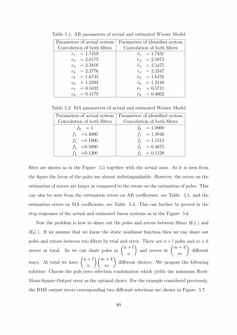
Table 5.1: AR parameters of actual and estimated Wiener Model
Parameters of actual system Parameters of identified systemConvolution of both filters Convolution of both filters
e1 = 1.7459 e1 = 1.7431e2 = 2.6175 e2 = 2.5873e3 = 2.5816 e3 = 2.5475e4 = 2.2776 e4 = 2.2347e5 = 1.6745 e5 = 1.6476e6 = 1.2392 e6 = 1.2148e7 = 0.5832 e7 = 0.5711e8 = 0.4170 e8 = 0.4062
Table 5.2: MA parameters of actual and estimated Wiener Model
Parameters of actual system Parameters of identified systemConvolution of both filters Convolution of both filters
f0 = 1 f0 = 1.0000
f1 =1.4000 f1 = 1.3846
f2 =1.1800 f2 = 1.1515
f3 =0.5000 f3 = 0.4675
f4 =0.1200 f4 = 0.1128
filter are shown as in the Figure 5.5 together with the actual ones. As it is seen from
the figure the locus of the poles are almost indistinguishable. However, the errors on the
estimation of zeroes are larger as compared to the errors on the estimation of poles. This
can also be seen from the estimation errors on AR coefficients, see Table 5.1, and the
estimation errors on MA coefficients, see Table 5.2. This can further be proved in the
step responses of the actual and estimated linear systems as in the Figure 5.6
Now the problem is how to share out the poles and zeroes between filters H1(.) and
H2(.). If we assume that we know the static nonlinear function then we can share out
poles and zeroes between two filters by trial and error. There are n+ l poles and m+ k
zeroes at total. So we can share poles in
(n+ l
n
)and zeroes in
(m+ k
m
)different
ways. At total we have
(n+ l
n
)(m+ k
m
)different choices. We propose the following
solution: Choose the pole/zero selection combination which yields the minimum Root-
Mean-Square Output error as the optimal choice. For the example considered previously,
the RMS output errors corresponding two different selections are shown in Figure 5.7.
80
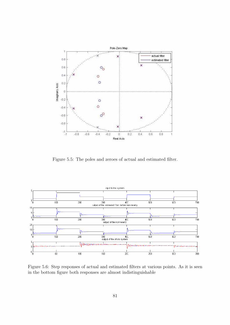
Figure 5.5: The poles and zeroes of actual and estimated filter.
Figure 5.6: Step responses of actual and estimated filters at various points. As it is seenin the bottom figure both responses are almost indistinguishable
81
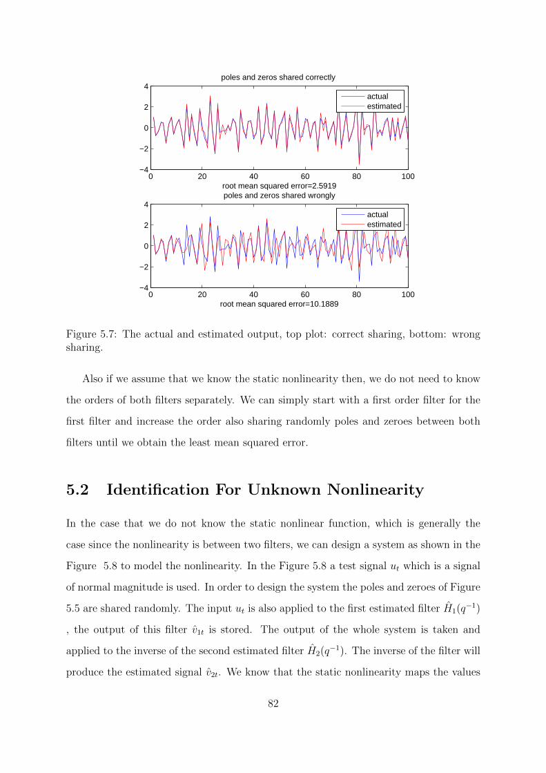
0 20 40 60 80 100−4
−2
0
2
4
root mean squared error=2.5919
poles and zeros shared correctly
actualestimated
0 20 40 60 80 100−4
−2
0
2
4
root mean squared error=10.1889
poles and zeros shared wrongly
actualestimated
Figure 5.7: The actual and estimated output, top plot: correct sharing, bottom: wrongsharing.
Also if we assume that we know the static nonlinearity then, we do not need to know
the orders of both filters separately. We can simply start with a first order filter for the
first filter and increase the order also sharing randomly poles and zeroes between both
filters until we obtain the least mean squared error.
5.2 Identification For Unknown Nonlinearity
In the case that we do not know the static nonlinear function, which is generally the
case since the nonlinearity is between two filters, we can design a system as shown in the
Figure 5.8 to model the nonlinearity. In the Figure 5.8 a test signal ut which is a signal
of normal magnitude is used. In order to design the system the poles and zeroes of Figure
5.5 are shared randomly. The input ut is also applied to the first estimated filter H1(q−1)
, the output of this filter v1t is stored. The output of the whole system is taken and
applied to the inverse of the second estimated filter H2(q−1). The inverse of the filter will
produce the estimated signal v2t. We know that the static nonlinearity maps the values
82
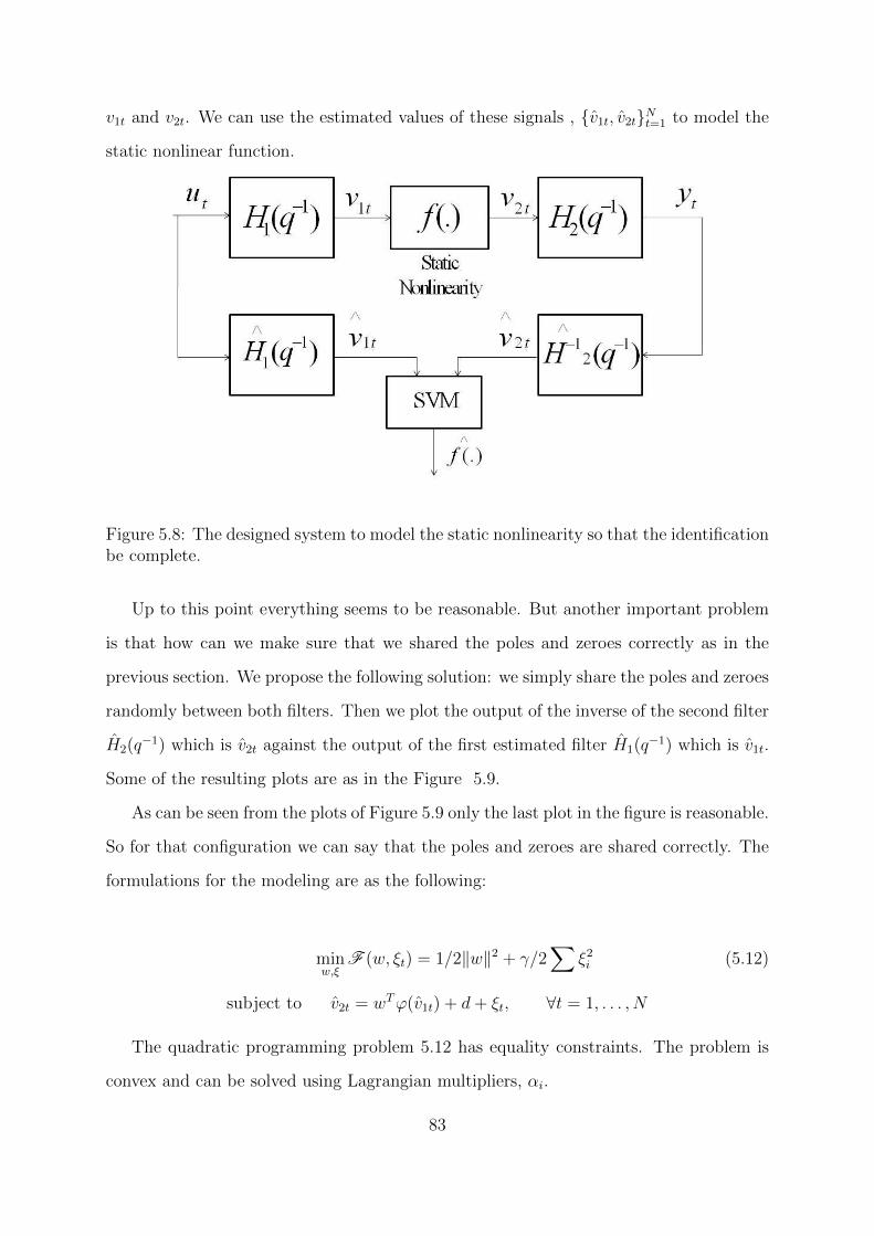
v1t and v2t. We can use the estimated values of these signals , v1t, v2tNt=1 to model the
static nonlinear function.
Figure 5.8: The designed system to model the static nonlinearity so that the identificationbe complete.
Up to this point everything seems to be reasonable. But another important problem
is that how can we make sure that we shared the poles and zeroes correctly as in the
previous section. We propose the following solution: we simply share the poles and zeroes
randomly between both filters. Then we plot the output of the inverse of the second filter
H2(q−1) which is v2t against the output of the first estimated filter H1(q
−1) which is v1t.
Some of the resulting plots are as in the Figure 5.9.
As can be seen from the plots of Figure 5.9 only the last plot in the figure is reasonable.
So for that configuration we can say that the poles and zeroes are shared correctly. The
formulations for the modeling are as the following:
minw,ξ
F (w, ξt) = 1/2‖w‖2 + γ/2∑
ξ2i (5.12)
subject to v2t = wTϕ(v1t) + d+ ξt, ∀t = 1, . . . , N
The quadratic programming problem 5.12 has equality constraints. The problem is
convex and can be solved using Lagrangian multipliers, αi.
83
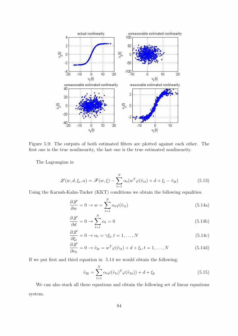
Figure 5.9: The outputs of both estimated filters are plotted against each other. Thefirst one is the true nonlinearity, the last one is the true estimated nonlinearity.
The Lagrangian is:
L (w, d, ξi, α) = F (w, ξ)−N∑t=1
αt(wTϕ(v1t) + d+ ξi − v2t) (5.13)
Using the Karush-Kahn-Tucker (KKT) conditions we obtain the following equalities.
∂L
∂w= 0 → w =
N∑t=1
αtϕ(v1t) (5.14a)
∂L
∂d= 0 →
N∑t=1
αt = 0 (5.14b)
∂L
∂ξt= 0 → αt = γξt, t = 1, . . . , N (5.14c)
∂L
∂αt
= 0 → v2t = wTϕ(v1t) + d+ ξt, t = 1, . . . , N (5.14d)
If we put first and third equation in 5.14 we would obtain the following:
v2k =N∑t=1
αtϕ(v1t)Tϕ(v1k)) + d+ ξk (5.15)
We can also stack all these equations and obtain the following set of linear equations
system.
84

0 1TN
1N K + γ−1I1TN
d
α
=
0
Y
(5.16)
Where K is a positive definite matrix and K(i, j) = ϕ(v1i))Tϕ(v1j)) = e(−‖v1i)−v1j)‖2)
, α = [α1 . . . αN ]T and d is the bias term. In (5.16) a least squares solution is obtained
in order to find α and d parameters. After obtaining these parameters, the resulting
expression for estimated function will be as the following:
v2t =N∑
k=1
αkK(v1t, v1k) + d, (5.17)
5.2.1 Example
In this example H1(q−1) and H2(q
−1) are chosen to be the same as in the Example
5.1.1. The nonlinearity is chosen as zk = 5 −0.5+11+e−0.5vk
. The length of training data used to
obtain the filter parameters is N = 200 , whereas it is chosen as N = 500 to model the
nonlinearity. The input signal ut has a Gaussian distribution of 0 mean and standard
deviation 2 while modeling the nonlinearity.
5.3 Black Box Identification of Wiener-Hammerstein
Models
In [19], Wiener-Hammerstein model is used to model paralyzed skeletal muscle and the
results are compared with the Hill Huxley model. We have also identified the Wiener-
Hammerstein model as a black box. We will compare the performances between these
approaches in terms of goodness of fit, (gof) and normalized mean approximation error
(nmae), where goodness of fit is defined as:
gof = 1−√∑N
k=1(y(k)− y(k))2∑Nk=1(y(k)− y(k))2
(5.18)
and nmae as:
85

nmae =1N
∑Nk=1 |(y(k)− y(k))|maxy(k) (5.19)
The corresponding performance values are shown in Table 5.3
Table 5.3: Goodness-of-fit (gof) and normalized mean absolute error (nmae) of the pro-posed model SVR model , LSL model and Hill Huxley model
SVR model LSL model Hill-Huxley modelgof nmae gof nmae gof nmae
0.8507 3.93% 0.7563 5.90 % 0.8426 0.09 %0.6580 3.93% 0.6457 9.30% 0.6539 1.02%
SVR model is better than Linear-Saturation-Linear (LSL) model in terms of nmae .
Hill Huxley model is the best in terms of nmae. All of them are similar in terms of gof
performance.
86
Chapter 6
CONCLUSIONS
In this thesis, we investigated identification of various nonlinear systems, e.g. (NARX,
Hammerstein, Wiener, Wiener-Hammerstein systems). The identification is held follow-
ing construction of a dataset (i.e. pairs of inputs and outputs) from the system under
investigation. In this work, we focused on using Least Squares-Support Vector Ma-
chines (LS-SVM) to identify these types of systems. We also designed closed loop control
schemes using LS-SVM.
In the first part of this thesis, we dealed with regression of nonlinear systems such
as Nonlinear Auto-Regressive with eXogenous inputs (NARX) and Bilinear systems. By
means of Least-Squares Support Vector Regression (LS-SVR) we developed new formu-
lations that decreased the mean squared error between actual and estimated outputs of
these type of systems. Through our simulations, we observed that usual SVR regression
method can not reach the performance of the Neural Network approximators. However
our formulations lead a comparable performance for training, and is better in terms of
test data error compared to Neural Network approximators.
In many works in the literature, the orders of the filter in nonlinear systems are
assumed to be known. Based on Least-Squares Support Vector Regression we showed
that we can determine these orders. The true orders are given in terms of percentages
and the proposed method may require a huge number of training data.
In the chapter 4 we dealed with parametric identification of Hammerstein and Wiener
87
type of systems. Identification of Hammerstein systems by LS-SVM requires that the
nonlinearity be non-static, i.e. memoryless. We have shown that we can still identify
Hammerstein systems for the case that the nonlinearity has a finite memory.
The methodology proposed in [1] for identification of Wiener type of systems, which
is to change the roles of inputs and outputs , hence making it a Hammerstein systems,
leads poor estimation results. We have shown that this is due to the unconsidered uncol-
ored noise, that is mapped to an infinite dimensional space by kernel functions of Support
Vectors. We have developed new approaches that improved the estimation performance
significantly. The ideas are based on using small signal analysis, hence making the over-
all system linear. At first, we shoved that the nonlinearity need not to be invertible, as
required in many works in the literature, assuming there is no measurement error. We
further developed the methodology such that we proposed novel schemes for the iden-
tification of Wiener type systems for any differentiable and non-differentiable nonlinear
functions.
We also designed feedback control schemes for Wiener type systems, by putting SVM
in appropriate places in the designed system, and showed that SVM can be used for
applying the well known linear control theory.
In the chapter 5 we have concentrated on identification of Wiener-Hammerstein type
systems by using LS-SVM, which is set as a future problem in [1]. Using similar ideas
explained in the identification of Wiener type systems, we identified Wiener-Hammerstein
type systems for both the cased that the nonlinearity between the linear blocks is known or
unknown. Finally we proposed novel schemes for the identification of Wiener-Hammerstein
type systems as a black box and compared the results with various works in the literature.
Throughout the thesis we considered Single-Input, Single-Output (SISO), Discrete
Time Systems. The extension of the schemes proposed in this thesis to Multi-Input
and/or Multi-Output cases seem to be straightforward. However, this point requires
further investigation.
Our methodology to determine the orders of the filters in the nonlinear systems may
further be improved to determine the orders of any type of nonlinear system. The systems
88

that we dealed in this thesis are in the open loop form. The methodologies may further be
modified to identify closed loop forms of these type of systems, such as closed loop Wiener,
Hammerstein (i.e. Lur’e model), see e.g. [41], and closed loop Wiener-Hammerstein
systems.
89
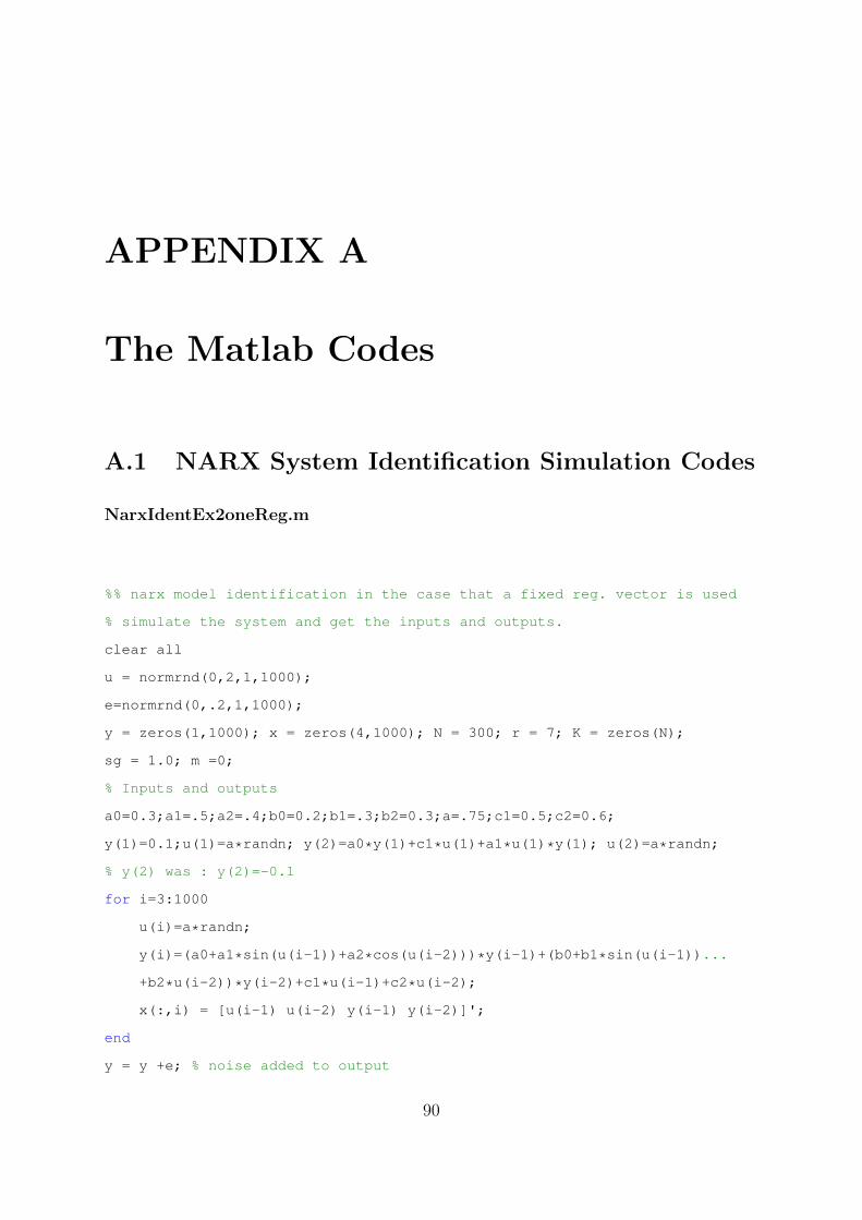
APPENDIX A
The Matlab Codes
A.1 NARX System Identification Simulation Codes
NarxIdentEx2oneReg.m
%% narx model identification in the case that a fixed reg. vector is used
% simulate the system and get the inputs and outputs.
clear all
u = normrnd(0,2,1,1000);
e=normrnd(0,.2,1,1000);
y = zeros(1,1000); x = zeros(4,1000); N = 300; r = 7; K = zeros(N);
sg = 1.0; m =0;
% Inputs and outputs
a0=0.3;a1=.5;a2=.4;b0=0.2;b1=.3;b2=0.3;a=.75;c1=0.5;c2=0.6;
y(1)=0.1;u(1)=a*randn; y(2)=a0*y(1)+c1*u(1)+a1*u(1)*y(1); u(2)=a*randn;
% y(2) was : y(2)=-0.1
for i=3:1000
u(i)=a*randn;
y(i)=(a0+a1*sin(u(i-1))+a2*cos(u(i-2)))*y(i-1)+(b0+b1*sin(u(i-1))...
+b2*u(i-2))*y(i-2)+c1*u(i-1)+c2*u(i-2);
x(:,i) = [u(i-1) u(i-2) y(i-1) y(i-2)]';
end
y = y +e; % noise added to output
90

figure(1);subplot(2,1,1);plot(u);title('u : input values');subplot(2,1,2);
plot(y);title('y : output values');
% Construct kernel and other required matrices
xtrain = x(:,201:200+N); ytrain = y(201:200+N);
for i = 1:N
for j = 1:N
K(i,j) = exp(-(( norm( x(:,200+i) - x(:,200+j) ) )ˆ2)/(2*sgˆ2));
end
end
Ksus = K(r:N,r:N);
%Construct Ko
Ko = zeros(N-r+1,m+1);
for k = r:N
Ko(k-r+1,1) = sum(K(:,k));
end
% Construct YpUp and Yf
for i = 1:2
Yp(i,:) = y(200+r-i:200+N-i);
Up(i,:) = u(200+r-i:200+N-i);
end
YpUp = [Yp;Up];
Yf = y(200+r:200+N);
gm = 1500;
bigEqMat = ...
[ 0 0 0 0 0 ones(N-r+1,1)' 0 ;...
zeros(4,1) zeros(4,4) YpUp zeros(4,1) ;...
ones(N-r+1,1) YpUp' Ksus + (1/gm)*eye(N-r+1) Ko ;...
0 0 0 0 0 Ko' ones(1,N)*K*ones(N,1) ];
%solve linear equation
rigSide = [0 0 0 0 0 Yf 0]';
finSolution = bigEqMat\rigSide;d1 = finSolution(1)
a es = finSolution(2:5)
alf = finSolution(6:end-1);
bet1 = finSolution(end)
91

y es(1:20) = y(1:20);xtest = [y es(20) y es(19) u(20) u(19)]';
for t = 21:1000
y es(t) = a es(1)*y es(t-1) + a es(2)*y es(t-2)+a es(3)*u(t-1)+...
a es(4)*u(t-2)...;
+ svm out(xtest,xtrain,bet1,alf,d1,sg,r) ;
xtest = [y(t) y(t-1) u(t) u(t-1)]';
end
figure(2);plot(y es(500:650),'r:');hold on ;plot(y(500:650),'b:');
title('estimated output using one reg. vector');
legend('estimated model','actual model');grid;hold off;
%For for loop just below obtain training performance, the previous for loop
%seems not to do that
y es(1:200) = y(1:200);xttest = [y(200) y(199) u(200) u(199)]';
for t = 201:200+N
y es(t) = a es(1)*y(t-1) + a es(2)*y(t-2)+a es(3)*u(t-1)+a es(4)*u(t-2)...;
+ svm out(xttest,xtrain,bet1,alf,d1,sg,r) ;
xttest = [y(t) y(t-1) u(t) u(t-1)]';
end
%% PERFORMANCES: MSE, REGRESSION etc, output and target plots. for test tr.
rmse train =sqrt(mean( (y(201:200+N)-y es(201:200+N)).ˆ2 ))
figure(3);
subplot(2,1,1);plot(y(201:200+N));hold on;plot(y es(201:200+N),'r');
title(['RMSE of Training: ',num2str(rmse train)]);hold off
rmse test =sqrt(mean( (y(200+N:200+N+N)-y es(200+N:200+N+N)).ˆ2 ))
subplot(2,1,2);plot(y(200+N:200+N+N));hold on;plot(y es(200+N:200+N+N),'r')
title(['RMSE of Test:',num2str(rmse test)])
figure(4);title('Correlation between actual and estimated outputs, SVR-1K')
subplot(1,2,1);plot(y(201:200+N),y es(201:200+N),'bo');hold on ;
ezplot('x','r',[-4 10 -4 10])
reg train =corrcoef( y(201:200+N-100)',y es(201:200+N-100)' )
reg test =corrcoef( y(200+N:200+N+200)',y es(200+N:200+N+200)' )
NARXIdentEx2.m
92
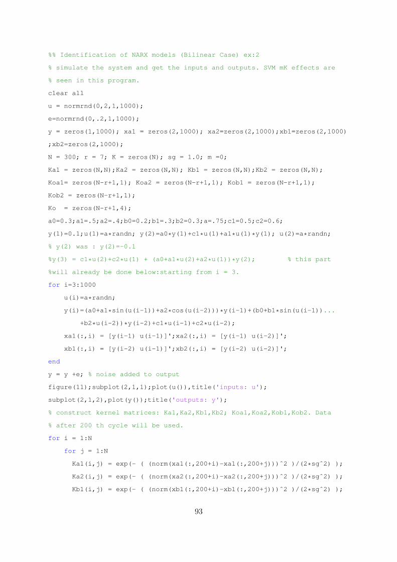
%% Identification of NARX models (Bilinear Case) ex:2
% simulate the system and get the inputs and outputs. SVM mK effects are
% seen in this program.
clear all
u = normrnd(0,2,1,1000);
e=normrnd(0,.2,1,1000);
y = zeros(1,1000); xa1 = zeros(2,1000); xa2=zeros(2,1000);xb1=zeros(2,1000)
;xb2=zeros(2,1000);
N = 300; r = 7; K = zeros(N); sg = 1.0; m =0;
Ka1 = zeros(N,N);Ka2 = zeros(N,N); Kb1 = zeros(N,N);Kb2 = zeros(N,N);
Koa1= zeros(N-r+1,1); Koa2 = zeros(N-r+1,1); Kob1 = zeros(N-r+1,1);
Kob2 = zeros(N-r+1,1);
Ko = zeros(N-r+1,4);
a0=0.3;a1=.5;a2=.4;b0=0.2;b1=.3;b2=0.3;a=.75;c1=0.5;c2=0.6;
y(1)=0.1;u(1)=a*randn; y(2)=a0*y(1)+c1*u(1)+a1*u(1)*y(1); u(2)=a*randn;
% y(2) was : y(2)=-0.1
%y(3) = c1*u(2)+c2*u(1) + (a0+a1*u(2)+a2*u(1))*y(2); % this part
%will already be done below:starting from i = 3.
for i=3:1000
u(i)=a*randn;
y(i)=(a0+a1*sin(u(i-1))+a2*cos(u(i-2)))*y(i-1)+(b0+b1*sin(u(i-1))...
+b2*u(i-2))*y(i-2)+c1*u(i-1)+c2*u(i-2);
xa1(:,i) = [y(i-1) u(i-1)]';xa2(:,i) = [y(i-1) u(i-2)]';
xb1(:,i) = [y(i-2) u(i-1)]';xb2(:,i) = [y(i-2) u(i-2)]';
end
y = y +e; % noise added to output
figure(11);subplot(2,1,1);plot(u()),title('inputs: u');
subplot(2,1,2),plot(y());title('outputs: y');
% construct kernel matrices: Ka1,Ka2,Kb1,Kb2; Koa1,Koa2,Kob1,Kob2. Data
% after 200 th cycle will be used.
for i = 1:N
for j = 1:N
Ka1(i,j) = exp(- ( (norm(xa1(:,200+i)-xa1(:,200+j)))ˆ2 )/(2*sgˆ2) );
Ka2(i,j) = exp(- ( (norm(xa2(:,200+i)-xa2(:,200+j)))ˆ2 )/(2*sgˆ2) );
Kb1(i,j) = exp(- ( (norm(xb1(:,200+i)-xb1(:,200+j)))ˆ2 )/(2*sgˆ2) );
93
Kb2(i,j) = exp(- ( (norm(xb2(:,200+i)-xb2(:,200+j)))ˆ2 )/(2*sgˆ2) );
end
end; xtraina1 = xa1(:,201:200+N);xtraina2 = xa2(:,201:200+N);
xtrainb1 = xb1(:,201:200+N);xtrainb2 = xb2(:,201:200+N);
for t =1:N-r+1
Koa1(t,1) = sum(Ka1(t,:));
%since it is symmetric otherwise will also be the same. for all!..
Koa2(t,1) = sum(Ka2(t,:));
Kob1(t,1) = sum(Kb1(t,:));
Kob2(t,1) = sum(Kb2(t,:));
end
Ko = [Koa1 Koa2 Kob1 Kob2];
% Construct Ksus.
Ksus=Ka1(r:end,r:end)+Ka2(r:end,r:end)+Kb1(r:end,r:end)+Kb2(r:end,r:end);
% Construct YpUp and Yf
for i = 1:2
Yp(i,:) = y(200+r-i:200+N-i);
Up(i,:) = u(200+r-i:200+N-i);
end
YpUp = [Yp;Up];
Yf = y(200+r:200+N);
%% Construct the linear equation matrix and solve the equation
gm=1500; sumOmg =[sum(sum(Ka1)) sum(sum(Ka2)) sum(sum(Kb1)) sum(sum(Kb2))];
bigEqMat = [0 zeros(1,4) ones(1,N-r+1) zeros(1,4);...
zeros(4,1) zeros(4,4) YpUp zeros(4,4);...
ones(N-r+1,1) YpUp' Ksus+(1/gm)*eye(N-r+1) Ko ;...
zeros(4,1) zeros(4,4) Ko' diag(sumOmg)];
% diag(sumOmg)
rightSide = [0 zeros(1,4) Yf zeros(1,4) ]'; %
finSolution = bigEqMat\rightSide;% partition the finSolution.
d = finSolution(1,1)
a es = finSolution(2:5,1) %estimaded a s
94
alf = finSolution(6:end-4,1);
bet = finSolution(end-3:end,1);a0 es = a es(1);b0 es = a es(2);
c1 es = a es(3);c2 es = a es(4);
%% Now try to obtain the estimated nonlinearity values
for k = 1:N-r+1
fa1 es(k) = alf'*Ka1(r:end,k+r-1);
fa2 es(k) = alf'*Ka2(r:end,k+r-1);
fb1 es(k) = alf'*Kb1(r:end,k+r-1);
fb2 es(k) = alf'*Kb2(r:end,k+r-1);
end
figure(12); plot3(xa1(1,200+r:200+N),xa1(2,200+r:200+N),fa1 es,'r+');
grid on;xlabel('X');ylabel('Y');zlabel('Z');
hold on;plot3(xa2(1,200+r:200+N),xa2(2,200+r:200+N),fa2 es,'g+');
xlabel('X');ylabel('Y');zlabel('Z');hold off
% figure(4); plot3(xa2(1,200+r:200+N),xa2(2,200+r:200+N),fa2 es,'r+');
%grid;xlabel('X');ylabel('Y');zlabel('Z');
% figure(5); plot3(xb1(1,200+r:200+N),xb1(2,200+r:200+N),fb1 es,'r+');
%grid;xlabel('X');ylabel('Y');zlabel('Z');
% figure(6); plot3(xb2(1,200+r:200+N),xb2(2,200+r:200+N),fb2 es,'r+');
%grid;xlabel('X');ylabel('Y');zlabel('Z');
% figure(7); ribbon(xb2(1,200+r:200+N),fb2 es);
%% now try to obtain nonlinearity term parameters(coefficients).
finSola1d1 = [xa1(1,200+r:200+N)'.*xa1(2,200+r:200+N)'...
-ones(N-r+1,1)]\fa1 es',d1 = finSola1d1(2);
finSola2d2 = [xa2(1,200+r:200+N)'.*xa2(2,200+r:200+N)'...
-ones(N-r+1,1)]\fa2 es',d2 = finSola2d2(2);
finSolb1d3 = [xb1(1,200+r:200+N)'.*xb1(2,200+r:200+N)'...
-ones(N-r+1,1)]\fb1 es',d3 = finSolb1d3(2);
finSolb2d4 = [xb2(1,200+r:200+N)'.*xb2(2,200+r:200+N)'...
-ones(N-r+1,1)]\fb2 es',d4 = finSolb2d4(2);
% The results seems to be satisfactory for the paragraph just above.
%% Now obtain the estimated model's output. the inputs following training
% set can be used for testing. but no need for that! we can start fr begin.
y es(1:20) = y(1:20);xa1test = [y es(20) u(20)]';xa2test = [y es(20) u(19)]';
xb1test = [y es(19) u(20)]';xb2test = [y es(19) u(19)]';
95
% below instead of d/4 we could use d1,d2,d3and d4 .result is almost the
% same.
for k = 21:900
y es(k) = a0 es*y es(k-1) + b0 es*y es(k-2) + c1 es*u(k-1) +c2 es*u(k-2)...;
+ svm out(xa1test,xtraina1,bet(1),alf,d/4,sg,r) +...
svm out(xa2test,xtraina2,bet(2),alf,d/4,sg,r)...;
+ svm out(xb1test,xtrainb1,bet(3),alf,d/4,sg,r) +...
svm out(xb2test,xtrainb2,bet(4),alf,d/4,sg,r);
xa1test = [y es(k) u(k)]'; xa2test = [y es(k) u(k-1)]';
xb1test = [y es(k-1) u(k)]';xb2test = [y es(k-1) u(k-1)]';
end
figure(13);plot(y es(500:800),'r:');hold on ;plot(y(500:800),'b-.');grid;hold off;
legend('estimated model','actual model');title('estimated and actual model outputs');
%For for loop just below obtain training performance, the previous for loop
%seems not to do that
y es(1:200) = y(1:200);xa1test = [y(200) u(200)]';xa2test = [y(200) u(199)]';
xb1test = [y(199) u(200)]';xb2test = [y(199) u(199)]';
% below instead of d/4 we could use d1,d2,d3and d4 .result is almost the
% same.
for k = 201:200+N
y es(k) = a0 es*y(k-1) + b0 es*y(k-2) + c1 es*u(k-1) +c2 es*u(k-2)...;
+ svm out(xa1test,xtraina1,bet(1),alf,d/4,sg,r) +...
svm out(xa2test,xtraina2,bet(2),alf,d/4,sg,r)...;
+ svm out(xb1test,xtrainb1,bet(3),alf,d/4,sg,r) +...
svm out(xb2test,xtrainb2,bet(4),alf,d/4,sg,r);
xa1test = [y(k) u(k)]'; xa2test = [y(k) u(k-1)]';
xb1test = [y(k-1) u(k)]';xb2test = [y(k-1) u(k-1)]';
end
%% PERFORMANCES: MSE, REGRESSION etc, output and target plots. for test tr.
rmse train =sqrt(mean( (y(201:200+N)-y es(201:200+N)).ˆ2 ))
figure(14);
subplot(2,1,1);plot(y(201:200+N));hold on;plot(y es(201:200+N),'r');
title(['RMSE of Training: ',num2str(rmse train)])
rmse test =sqrt(mean( (y(200+N:200+N+300)-y es(200+N:200+N+300)).ˆ2 ))
subplot(2,1,2);plot(y(200+N:200+N+300));hold on;plot(y es(200+N:200+N+300),'r');
96
title(['RMSE of Test:',num2str(rmse test)]);hold off
figure(15);title('Correlation between actual and estimated outputs, SVR-mK');
subplot(1,2,2);plot(y(201:200+N),y es(201:200+N),'bo');hold on ;
ezplot('x','r',[-4 10 -4 10]);
reg train =corrcoef( y(201:200+N-200)',y es(201:200+N-200)' )
reg test =corrcoef( y(200+N:200+N+100)',y es(200+N:200+N+100)' )
svm out.m
%% now we will produce a function that computes the output of the svm
%% directly. that is w'*fi(x) + d.
function [val] = svm out(xtest,xtrain,bet,alph,d,sg,r)
%xtrain: xtrain must be in this form. each column is a seperate training
%data. it is assumed to be in this form.
%xtest : xtest is also in the form of xtrain. that is columns are seperate
%training datas.
%alph : is assumed to be in column.
%first we have to compute the kernel matrix. K is N by 1 in this case.
%first of all obtain the size of training data thus the kernel matrix
[m,n] = size(xtrain);
if(m>n)
sizeK = m;
else
sizeK = n;
end
K=zeros(sizeK,1);
for i = 1:sizeK
K(i,1) = exp(- ((norm( xtrain(:,i) - xtest ))ˆ2)/(2*sgˆ2) );
% Be carefull with the value of sg or sgˆ2
end
val = bet*sum(K(:,1)) + alph'*K(r:end,1) + d;
97
A.2 Wiener System Identification Simulation Codes
WienerAsAHammersteinAnyNon.m
%% Wiener identification : thinking it as a Hammerstein model. Using small
%% signal analysis. here a stepwise constant is added to input. But the
%% results seem to be nice for denumerator paramters not good for numerator
%% parameters.( this has changed. because wrong calculations were done at
%% that time) In the case that the nonlinearity is not invertible around
%% zero. Noise exist in the output. A working condition is constructed.
%% Wait for the transient time and after some time (200 possibly) evaluate
%% mean of the things. The training data also should be chosen after the
%% transient time. Increasing the training data gave worse results.
%% Decreasing it below some points also gave worse results.
clear all
u=.35*normrnd(0,.32,1,700) + 24; % A white gaussian input sequence u with length
%700 0 mean and standard deviation 2
%u=8*rand(1,700)-4;
e=.05*normrnd(0,.2,1,1189); % A white gaussian with zero mean and standart de
% viation .2 with length 700. it is error term
%e = zeros(1,1189); % this is added after all. actually it should have
ic = i; % been done before
rts = [.98*exp(ic) .98*exp(-ic) .98*exp(1.6*ic) .98*exp(-1.6*ic)...
.95*exp(2.5*ic) .95*exp(-2.5*ic)];
a = poly(rts); % ai s
b = [1 .8 .3 .4] ; % bi s
% now we will get the input output data.
[h,tt] = impz(b,[a]); %filter impulse response
us = [0 u(1:end-1)]; % past values of "u"
v = conv(h,u); v2 = (sin(u).*u) ; y2 = conv(h,v2);figure(50);
plot(u,v2,'r+');title('v2 vs u . hammersteinish ');
y =(sin(v).*v)+e; % y = conv(h,v2); % 3*(-.5 + 1./(1 + exp(-.5*v)));%2*v;
y y2diff = y-y2;figure(51);subplot(4,1,4); plot(y y2diff(1:700));
title('y-y2: wiener output-hammerstein output')
98
figure(1);subplot(3,1,1) ; plot(u(1:700)); title('input to the system');
subplot(3,1,2) ; plot(v(1:700));
title('output of the filter of wiener: before nonlinearity: v');
axis([1 700 -2 12])
subplot(3,1,3) ; plot(y(1:700));
title('output of the whole system of wiener');hold off
%subplot(4,1,4) ; plot(y2(1:700));
%title('output of the whole system of hammerstein; y2');
N=400; r=7; m=3;n= sum(size(a))-2; sg = .7071;
%% solve linear equation
% construct Kernel matrix . The last two hundred data points will be used.
xtrain = u(201:200+N);
for i=1:N % K is omega matrix
for j=1:N
K(i,j) = exp(-((u(1,i+200)-u(1,j+200))ˆ2)/(2*sgˆ2)); %itis oki
end
end
% Construct Yf. Again the last two hundred data points will be used .
Yf = y(1,200+r:200+N)-mean(y(200:700)); %it is okei
% Construct Yp:n*N-r+1. Again the last two hundred data points will be used.
for i=1:n
Yp(i,1:N-r+1) = y(1,200+r-i:N+200-i); %itis okei
end
% Construct Ko. Ko:194*4 (expected) it is okei.
for p = 1:N-r+1
for q = 1:m+1
sumk = 0;
for t = 1:N
sumk = sumk + K(t,r+p-q);
end
Ko(p,q) = sumk;
end
end
% Construct Ksus . Ksus:194*194 (expected, not sure): well Ksus2 = Ksus .
% it is great.
99
for p = 1:N-r+1
for q = 1:N-r+1
sumks = 0;
for j =0:m % 0 dan 3 e olmas? gerekti?i tespit edilmi?ti.
sumks = sumks + K(p+7-j-1,q+7-j-1);
end
Ksus2(p,q) = sumks;
end
end
Ksus = zeros(N-r+1); ud =u(1,201:200+N)'; yd =y(1,201:200+N); %it is okei
for j=0:m
Ksus = Ksus + kernel matrix(ud(r-j:N-j),'RBF kernel',2*sgˆ2);
end;
%% Construct the linear equation matrix (205 by 205) and solve the equation
gm = 500;
bigEqMat = [0 zeros(1,n) ones(1,N-r+1) zeros(1,m+1);...
zeros(n,1) zeros(n,n) Yp zeros(n,m+1);...
ones(N-r+1,1) Yp' Ksus+(1/gm)*eye(N-r+1,N-r+1) Ko;...
zeros(m+1,1) zeros(m+1,n) Ko' ones(1,N)*K*ones(N,1)*eye(m+1,m+1)];
rightSide = [0 zeros(1,n) Yf zeros(1,m+1) ]';
finSolution = bigEqMat\rightSide;% partition the finSolution.
d = finSolution(1,1)
a es = finSolution(2:n+1,1) %estimaded a s
alf = finSolution(n+2:N+1,1);
bet = finSolution(N+2:N+5,1);
%% Get the solutions for b s .
AlfM = [alf(end:-1:1,1)' 0 0 0;0 alf(end:-1:1,1)' 0 0;...
0 0 alf(end:-1:1,1)' 0 ;0 0 0 alf(end:-1:1,1)']; %Alfa matrix
%Construct Manipulated Kernel matrix
for i = 1:N-m
Kman(i,:) = K(N-i+1,:);
end
% Get the right hand side of matrix of which svd is to be taken
100
svdRight = AlfM*Kman + bet*sum(K);
[B , s, F] = svd(svdRight);
nf = s(1,1)*F(:,1); %fvec
b es = B(:,1)'; %bvec
meanf= d/sum(b es); %fmean
multm= b es;
esf = (nf + meanf)*multm(1);
b es = b es/multm(1)
figure(3);
plot(ud(:,1),esf(:,1),'r+'); title('estimated f vs inputs')
grid
figure(11); plot(ud(:,1),svdRight(1,:),'m+');grid;
title('w0''f(ut) vs ut');
sys or=tf([b],[a],-1);
sys es=tf([b es],[1 -a es'],-1);
figure(44);pzmap(sys or,'r',sys es,'b');
legend('actual filter','estimated filter');
figure(45);subplot(1,2,1);hist(xtrain,18);
title('histogram of input data');
subplot(1,2,2);hist(Yf,18);title('histogram of output data');
%% We are not done. We have to obtain the whole static nonlinear function.
%% Estimated and actual filters are connected feedforwardly and SVM is
%% trained with those data.
%% we found filter parameters and now we have to find the nonlinearity.
%------now get the estimated filter's output and find nonlinearity- 1st
%check the nonlinear function used above!!! then use the same one here
u n = 1*normrnd(0,1,1,700); %input used for obtaining the nonlinear funct
v n = conv(h,u n);
y n =(sin(v n).*v n)+e ;
[hes,ttes] = impz(b es,[1 -a es']);%estimated filter impulse response
ves = conv(hes,u n);
% now from estimated filter's outputs(ves) we will compute Kernel K
xtraines = ves(201:200+N);
101
for i=1:N % K is omega matrix
for j=1:N
Kes(i,j) = exp(-((ves(1,i+200)-ves(1,j+200))ˆ2)/(1*1ˆ2));%itis oki
end
end
gm = 1600;
RegMat = [0 ones(N,1)';ones(N,1) Kes+(1/gm)*eye(N)];
regRightSide = [0;y n(201:200+N)'];
regFinSol = RegMat\regRightSide;des = regFinSol(1)
alfes=regFinSol(2:end);
for k=1:N
yes(k) = alfes'*Kes(:,k) + des;
end
figure(71);subplot(3,1,1) ; plot(u n(1:700)); title('input to the system');
subplot(3,1,2) ; plot(v n(1:700));
title('output of the filter: before nonlinearity');
subplot(3,1,3) ; plot(ves(1:700));
title('output of the estimated filter: before nonlinearity');
figure(72);subplot(3,1,1) ;plot(u n(1:200)); title('input to the system');
subplot(3,1,2) ; plot(y n(1:200)); title('output of the whole system');
%subplot(3,1,3) ; plot(yes(1:200));title('output of the estimated model');
figure(73);plot(xtraines,yes,'r.');hold on;
plot(v n(201:200+N),y n(201:200+N),'b.');
title('actual and estimated nolinearities')
legend('estimated nonlinearity','actual nonlinearity');grid;hold off
rmse Non Fun = sqrt(mean( (yes - y n(201:200+N)).ˆ2 ))
PE AR = norm(a-[1 -a es'])
PE MA = norm(b-b es)
kernel matrix.m
102
function omega = kernel matrix(Xtrain,kernel type, kernel pars,Xt)
% Construct the positive (semi-) definite and symmetric kernel matrix
%
% >> Omega = kernel matrix(X, kernel fct, sig2)
%
% This matrix should be positive definite if the kernel function
% satisfies the Mercer condition. Construct the kernel values for
% all test data points in the rows of Xt, relative to the points of X.
%
% >> Omega Xt = kernel matrix(X, kernel fct, sig2, Xt)
%
%
% Full syntax
%
% >> Omega = kernel matrix(X, kernel fct, sig2)
% >> Omega = kernel matrix(X, kernel fct, sig2, Xt)
%
% Outputs
% Omega : N x N (N x Nt) kernel matrix
% Inputs
% X : N x d matrix with the inputs of the training data
% kernel : Kernel type (by default 'RBF kernel')
% sig2 : Kernel parameter (bandwidth in the case of the 'RBF kernel')
% Xt(*) : Nt x d matrix with the inputs of the test data
%
% See also:
% RBF kernel, lin kernel, kpca, trainlssvm, kentropy
% Copyright (c) 2002, KULeuven-ESAT-SCD, License & help @ http://www.esat.kuleuven.ac.be/sista/lssvmlab
nb data = size(Xtrain,1);
103
if nb data> 3000,
error(' Too memory intensive, the kernel matrix is restricted to size 3000 x 3000 ');
end
%if size(Xtrain,1)<size(Xtrain,2),
% warning('dimension of datapoints larger than number of datapoints?');
%end
if strcmp(kernel type,'RBF kernel'),
if nargin<4,
XXh = sum(Xtrain.ˆ2,2)*ones(1,nb data);
omega = XXh+XXh'-2*Xtrain*Xtrain';
omega = exp(-omega./kernel pars(1));
else
XXh1 = sum(Xtrain.ˆ2,2)*ones(1,size(Xt,1));
XXh2 = sum(Xt.ˆ2,2)*ones(1,nb data);
omega = XXh1+XXh2' - 2*Xtrain*Xt';
omega = exp(-omega./kernel pars(1));
end
else
if nargin<4,
omega = zeros(nb data,nb data);
for i=1:nb data,
omega(i:end,i) = feval(kernel type, Xtrain(i,:), Xtrain(i:end,:),kernel pars);
omega(i,i:end) = omega(i:end,i)';
end
else
if size(Xt,2) 6=size(Xtrain,2),
error('dimension test data not equal to dimension traindata;');
end
omega = zeros(nb data, size(Xt,1));
104
for i=1:size(Xt,1),
omega(:,i) = feval(kernel type, Xt(i,:), Xtrain, kernel pars);
end
end
end
A.3 Wiener-Hammerstein System Identification Sim-
ulation Codes
WienerHammersteinIdent.m
%% Wiener - Hammerstein Identification (by convolution and small signal
%% analysis )
clear all
b1 = [1 .8 .3]; ic =i;
a1 = poly([.78*exp(ic) .78*exp(-ic) .88*exp(1.6*ic) .88*exp(-1.6*ic)]);
a2 = poly([.98*exp(2*ic) .98*exp(-2*ic) .96*exp(3.6*ic) .96*exp(-3.6*ic)]);
b2 = [1 .6 .4];
a = (poly([roots(a1)' roots(a2)']))',b = (poly([roots(b1)' roots(b2)']))'
u = .2*normrnd(0,2,1,700);%u st = ones(1,700);
%e = .2*normrnd(0,.012,1,1265);
e = zeros(1,1265);
[h1,tt1] = impz(b1,a1);
[h2,tt2] = impz(b2,a2);
v = conv(h1,u); % output of 1st filter
w = 5*(-.5 + 1./(1 + exp(-.5*v)) );% 2*v;% (sin(v).*v)+4*v;% output of nonlinearity
y = conv(h2,w)+e; %output of 2nd filter.
figure(1);subplot(4,1,1) ; plot(u(1:700)); title('input to the system');
subplot(4,1,2) ; plot(v(1:700)); title('output of the filter: before nonlinearity');
subplot(4,1,3) ; plot(w(1:700)); title('output of the nonlinearity');
subplot(4,1,4) ; plot(y(1:700));title('output of the whole system');
105
N=200; r=9; m=4;n= sum(size([a1 a2]))-3; sg = 1/sqrt(2);
%% solve linear equation
% construct Kernel matrix . The last two hundred data points will be used.
xtrain = u(201:200+N);
for i=1:N % K is omega matrix
for j=1:N
K(i,j) = exp(-((u(1,i+200)-u(1,j+200))ˆ2)/(2*sgˆ2)); %itis oki
end
end
% Construct Yf. Again the last two hundred data points will be used .
Yf = y(1,200+r:200+N); %it is okei
% Construct Yp:n*N-r+1. Again the last two hundred data points will be used.
for i=1:n
Yp(i,1:N-r+1) = y(1,200+r-i:N+200-i); %itis okei
end
% Construct Ko. Ko:194*4 (expected) it is okei.
for p = 1:N-r+1
for q = 1:m+1
sumk = 0;
for t = 1:N
sumk = sumk + K(t,r+p-q);
end
Ko(p,q) = sumk;
end
end
% Construct Ksus . Ksus:194*194 (expected, not sure): well Ksus2 = Ksus .
% it is great.
for p = 1:N-r+1
for q = 1:N-r+1
sumks = 0;
for j =0:m % 0 dan 3 e olmas? gerekti?i tespit edilmi?ti.
sumks = sumks + K(p+r-j-1,q+r-j-1);
end
Ksus2(p,q) = sumks;
end
106
end
Ksus = zeros(N-r+1); ud =u(1,201:200+N)'; yd =y(1,201:200+N); %it is okei
for j=0:m
Ksus = Ksus + kernel matrix(ud(r-j:N-j),'RBF kernel',2*sgˆ2);
end;
%% Construct the linear equation matrix (205 by 205) and solve the equation
gm = 500;
bigEqMat = [0 zeros(1,n) ones(1,N-r+1) zeros(1,m+1);...
zeros(n,1) zeros(n,n) Yp zeros(n,m+1);...
ones(N-r+1,1) Yp' Ksus+(1/gm)*eye(N-r+1,N-r+1) Ko;...
zeros(m+1,1) zeros(m+1,n) Ko' ones(1,N)*K*ones(N,1)*eye(m+1,m+1)];
rightSide = [0 zeros(1,n) Yf zeros(1,m+1) ]';
finSolution = bigEqMat\rightSide;% partition the finSolution.
d = finSolution(1,1)
a es = finSolution(2:n+1,1) %estimaded a s
alf = finSolution(n+2:201,1);
bet = finSolution(202:end,1);
%% Get the solutions for b s .
AlfM = [alf(end:-1:1,1)' 0 0 0 0;0 alf(end:-1:1,1)' 0 0 0;...
0 0 alf(end:-1:1,1)' 0 0 ;0 0 0 alf(end:-1:1,1)' 0;0 0 0 0 alf(end:-1:1,1)'];%Alfa matrix
%Construct Manipulated Kernel matrix
for i = 1:N-m;
Kman(i,:) = K(N-i+1,:);
end
% Get the right hand side of matrix of which svd is to be taken
svdRight = AlfM*Kman + bet*sum(K);
[B , s, F] = svd(svdRight);
nf = s(1,1)*F(:,1); %fvec
b es = B(:,1)'; %bvec
meanf= d/sum(b es); %fmean
multm= b es;
esf = (nf + meanf)*multm(1);
107
b es = b es/multm(1)
figure(3);
plot(ud(:,1),esf(:,1),'r+'); title('estimated f vs inputs')
grid
figure(11); plot(ud(:,1),svdRight(1,:),'m+');grid; title('w0''f(ut) vs ut');
PE AR = norm(a-[1;-a es])
PE MA = norm(b-b es')
%% ----------------------------- The System is identified as a whole. We----
%% ----------------------------have to divide the whole filter somehow--------------------
rots a = roots([1;-a es]);rots b = roots([b es]);
ra1 es = rots a(5:end);a1 es = poly(ra1 es); rb1 es = rots b(1:2);
b1 es = poly(rb1 es);
ra2 es = rots a(1:4) ;a2 es = poly(ra2 es); rb2 es = rots b(3:4);
b2 es = poly(rb2 es);
%------now get the estimated filter's output and compare with the originals-
%u = 1*normrnd(0,2,1,700);%u st = ones(1,700);
u(1:100) = 1*ones(1,100); u(101:200)=4*ones(1,100); u(201:300)=2*ones(1,100);
u(301:400)= 1*ones(1,100); u(401:500)=3*ones(1,100);
u(501:600)=1*ones(1,100);u(601:700)=2*ones(1,100);
v = conv(h1,u); % output of 1st filter
w =2*v; % (sin(v).*v); % 3*(-.5 + 1./(1 + exp(-.5*v)) );%% output of nonlinearity
y = conv(h2,w); %output of 2nd filter.
figure(20);title('Responses for various steps');subplot(4,1,1) ;
plot(u(1:700)); title('input to the system');
subplot(4,1,2) ; plot(v(1:700)); title('output of the filter: before nonlinearity');
subplot(4,1,3) ; plot(w(1:700)); title('output of the nonlinearity');
subplot(4,1,4) ; plot(y(1:700));title('output of the whole system');
N=200; r=9; m=4;n= sum(size([a1 a2]))-3; sg = 5;
[h1es,tt1es] = impz(b1 es,a1 es);
[h2es,tt2es] = impz(b2 es,a2 es);
ves = conv(h1es,u); % output of 1st estimated filter
wes =2*ves;% (sin(ves).*ves); % 3*(-.5 + 1./(1 + exp(-.5*ves)) );
%output of nonlinearity
yes = conv(h2es,wes); %output of 2nd filter.
figure(21);subplot(4,1,1) ; plot(u(1:700)); title('input to the system');
108
subplot(4,1,2) ; plot(ves(1:700));
title('output of the estimated filter: before nonlinearity');
subplot(4,1,3) ; plot(wes(1:700)); title('output of the nonlinearity');hold off
subplot(4,1,4) ; plot(yes(1:700));title('output of the whole estimated system')
hold on; plot(y(1:700),'r');title('output of the whole system');
figure(22);subplot(4,1,4);plot(y(1:700)-yes(1:700));
title('difference between actual and estimated outputs')
%% ------------find a figure for step inputs of org. and estim. sys.--------
% Pole zero maps of original and estimated system
sys or=tf([b'],[a'],-1);
sys es=tf([b es],[1 -a es'],-1);
figure(34);pzmap(sys or,'r',sys es,'b');legend('actual filter','estimated filter');
%% Now we will share out poles and zeros between two filters.
%% We assume that we know the nonlinearity.
bf1 = poly(rb1 es); % the same with the actual
af1 = poly([ra1 es(1:2)' ra2 es(1:2)']);
af2 = poly([ra1 es(3:4)' ra2 es(3:4)']);
bf2 = poly(rb2 es);% the same with the actual
afc = (poly([roots(a1)' roots(a2)']))';bfc = (poly([roots(b1)' roots(b2)']))';
% whole a and b.
uf = 1.*normrnd(0,2,1,700);%u st = ones(1,700);
[hf1,tt1] = impz(bf1,af1); [h1 es,tt1]= impz(b1 es,a1 es);
[hf2,tt2] = impz(bf2,af2); [h2 es,tt2]= impz(b2 es,a2 es);
vfe = conv(hf1,uf); va = conv(h1,uf); v es = conv(h1 es,uf);
% output of 1st filter ;estimated, actual, well estimated.
wfe = 3*(-.5 + 1./(1 + exp(-.5*vfe)) ); wa = 3*(-.5 + 1./(1 + exp(-.5*va)) );
w es = 3*(-.5 + 1./(1 + exp(-.5*v es)) ); % 2*v; %(sin(v).*v)+4*v;
% output of nonlinearity, estimated, actual
yfe = conv(hf2,wfe); ya = conv(h2,wa); y es = conv(h2 es,w es);
%output of 2nd filter. estimated, actual, well estimated
figure(41);subplot(4,1,1) ; plot(uf(1:700)); title('input to the system');
subplot(4,1,2) ; plot(vfe(1:700)); title('output of the filter: before nonlinearity');
hold on;subplot(4,1,2); plot(va(1:700));legend('estimate','actual');
subplot(4,1,3) ; plot(wfe(1:700)); title('output of the nonlinearity');
109

hold on; subplot(4,1,3);plot(wa(1:700));legend('estimate','actual');
subplot(4,1,4) ; plot(yfe(1:700));title('output of the whole system');
hold on; subplot(4,1,4);plot(ya(1:700));legend('estimate','actual');hold off
rmse ya yfe = sqrt( sum( (yfe(1:100)-ya(1:100)).ˆ2 ) )
rmse ya y es= sqrt( sum( (y es(1:100)-ya(1:100)).ˆ2 ) )
figure(42); subplot(2,1,1); plot(ya(1:100)); hold on ;subplot(2,1,1);
plot(y es(1:100),'r'); legend('actual', 'estimated');
title('poles and zeros shared correctly ' )
xlabel(['root mean squared error=',num2str(rmse ya y es)])
subplot(2,1,2); plot(ya(1:100)); hold on ;subplot(2,1,2); plot(yfe(1:100),'r');
legend('actual', 'estimated');title('poles and zeros shared wrongly')
xlabel(['root mean squared error=',num2str(rmse ya yfe)]); hold off
%% Now we will construct some random filters from the pool of poles and
%% zeros. Then we will plot the output of inverse of the 2nd estimated
%% filter vs the output of 1st estimated filter. If the relationship is
%% reasonable then we will train svm with that data. Use filter function of
%% matlab. be careful with the chosen nonlinearity 5*(-.5 + 1./(1 +
%% exp(-.5*v f1act)) )
u test = 1*normrnd(0,2,1,700);
v f1act = filter(b1,a1,u test); % actual 1st filter's output
w act = 5*(-.5 + 1./(1 + exp(-.5*v f1act)) );% output of nonlin of actual system
y f2act = filter(b2,a2,w act); % output of whole actual system
a1f1 = poly([ra1 es(1:2)' ra2 es(1:2)']); % for 1st filter of 1st system
a1f2 = poly([ra1 es(3:4)' ra2 es(3:4)']); % for 2nd filter of 1st system
v1f1e = filter(bf1,a1f1,u test); % output of 1st filter of 1st system
y1f2e = filter(bf2,a1f2,y f2act); % output of inverse of 2nd filter of 1st system
a2f1 = poly([ra1 es(3:4)' ra2 es(1:2)']); % for 1st filter of 2nd system
a2f2 = poly([ra1 es(1:2)' ra2 es(3:4)']); % for 2nd filter of 2nd system
v2f1e = filter(bf1,a2f1,u test); % output of 1st filter of 2nd system
y2f2e = filter(a2f2,bf2,y f2act); % output of inverse of 2nd filter of 2nd system
vf1 = filter(bf1,a1 es,u test); % output of 1st filter of correctly estimated system
110

yf2 = filter(a2 es,bf2,y f2act);% output of inverse of 2nd filter of correctly estimated system
figure(61); subplot(2,2,1); plot(v f1act,w act,'b.');
title('actual nonlinearity');xlabel('v 1(t)'),ylabel('v 2(t)'); grid ;
subplot(2,2,2); plot(v1f1e,y1f2e,'b.');
title('unreasonable estimated nonlinearity');xlabel('v 1(t)'),ylabel('v 2(t)');grid;
subplot(2,2,3); plot(v2f1e,y2f2e,'b.');
title('unreasonable estimated nonlinearity');xlabel(' v 1(t)'),ylabel('v 2(t)');grid;
subplot(2,2,4); plot(vf1,yf2,'b.');
title('reasonable estimated nonlinearity');xlabel('v 1(t)')
ylabel('v 2(t)'); axis([-15 15 -3 3]); grid;
%% Now different from just above we will try particle swarm optimization
%% instead while sharing out poles and
%% zeros to see the performance.
% u test = .2*normrnd(0,2,1,700);
% a1f1 = poly([ra1 es(1:2)' ra2 es(1:2)']); % for 1st filter of 1st system
% a1f2 = poly([ra1 es(3:4)' ra2 es(3:4)']); % for 2nd filter of 1st system
% [h1f1,tt1] = impz(bf1,a1f1);
% [h1f2,tt2] = impz(bf2,a1f2);
% a2f1 = poly([ra1 es(3:4)' ra2 es(1:2)']); % for 1st filter of 2nd system
% a2f2 = poly([ra1 es(1:2)' ra2 es(3:4)']); % for 2nd filter of 2nd system
% [h2f1,tt1] = impz(bf1,a2f1);
% [h2f2,tt2] = impz(bf2,a2f2);
% v1f1e = conv(h1f1,u test); % output of 1st filter of 1st system
% w1f1e = 3*(-.5 + 1./(1 + exp(-.5*vfe)) ); % output of nonlinearity of 1st system
% y1f2e = conv(h1f2,w1f1e); % output of 2nd filter of 1st system
%
% v2f1e = conv(h2f1,u test); % output of 1st filter of 2nd system
% w2f1e = 3*(-.5 + 1./(1 + exp(-.5*vfe)) ); % output of nonlinearity of 2nd system
% y2f2e = conv(h2f2,w2f1e); % output of 2nd filter of 2nd system
111
Bibliography
[1] I. Goethals, Subspace identification for linear, Hammerstein and Hammerstein-
Wiener systems. Ph.d. thesis, Katholieke Universiteit Leuven, Leuven, Sep 2005.
[2] A. Zhu and T. J. Brazil, “An adaptive volterra predistorter for the linearization of
rf high power amplifiers.,” Eee Mtt Int Microw Symp Dig, vol. 1, no. 1, p. 461, 2002.
[3] T. Wiegren, “Convergence analysis of recursive-identification algorithms based on
the nonlinear wiener model.,” IEEE Trans. Automatic Control, vol. 39, pp. 2191–
2206, 1994.
[4] I. Hunter and M. Korenberg, “The identification of nonlinear biological systems:
Wiener and hammerstein cascade models,” Biol. Cybern, vol. 55, no. 5, pp. 135,44,
1986.
[5] A. Cesari, J. M. Dilhac, P. L. Gilabert, G. Montoro, and E. Bertran, “A fpga based
platform for fast prototyping of rf pa predistortion linearizers.,” Topical Symposium
on Power Amplifiers for Wireless Communications, pp. 265–268, 2007.
[6] S. Norquay, A. Palazoglu, and J. Romagnoli, “Model predictive control based on
wiener models,” Chemical Engineering Science, vol. 53, no. 5, p. 084, 1998.
[7] E. Bai, “Frequency domain identification of wiener models.,” Automatica, vol. 39,
no. 9, p. 1521, 2003.
[8] Y. Zhao, L. Y. Wang, G. G. Yin, and J. Zhang, “Identification of wiener systems
with binary-valued output observations.,” Automatica, vol. 43, no. 10, p. 1752, 2007.
112
[9] T. Wigren, “Avoiding ill-convergence of finite dimensional blind adaptation schemes
excited by discrete symbol sequences.,” Signal Processing, vol. 62, no. 2, p. 121, 1997.
[10] L. Piroddi and W. Spinelli, “An identification algorithm for polynomial narx models
based on simulation error minimization.,” International Journal of Control, vol. 76,
no. 17, pp. 1767–1781, 2003.
[11] X. Hua, “Modeling and control of bilinear system.,” Northeast Chemical Engineering
Institute Press, 1990.
[12] Z. Wang and H. Gu, “Parameter identification of bilinear system based on genetic
algorithm,” Springer Verlag, vol. 8, no. 3, pp. 83–91, 2007.
[13] Y. Zhu, “Estimation of an n-l-n hammerstein-wiener model,” Automatica, vol. 8,
no. 3, pp. 1607–1614, 2002.
[14] J. C. Gomez and E. Baeyens, “Identification of block-oriented nonlinear systems
using orthonormal bases,” Journal of Process Control, vol. 14, no. 6, pp. 1685–697,
2004.
[15] S. Ghosh and S. Maka, “Non-linear system identification using hammerstein and non-
linear feedback models with piecewise linear static maps .,” International Journal of
Control, vol. 74, no. 18, pp. 1807–1823, 2001.
[16] I. Goethals, K. Pelckmans, J. A. Suykens, and B. D. Moor, “Idenitification of
mimo hammerstein models using least-squares support vector machines,” Automat-
ica, vol. 41, no. 7, pp. 1263–1272, 2005b.
[17] H. Liang and B. Wang, “Identification of wiener models using support vector ma-
chine.,” Fifth International Conference on Natural Computation, vol. 43, no. 10,
p. 1752, 2009.
[18] I. Hunter and M. Korenberg, “Support vector method for identification of wiener
models,” Journal of Process Control, vol. 19, no. 1, pp. 1174,1181, 2009.
113
[19] E.-W. Bai, Z. Cai, S. Dudley-Javoroski, and R. K. Shields, “Application of wiener-
hammerstein system identification in electrically stimulated paralyzed skeletal mus-
cle modeling.,” Automatica, vol. 45, no. 0191-2216, pp. 3305 – 3310, 2008.
[20] Cooper and M. Geoffrey, The Cell A Molecular Approach. No. 3, Sunderland: MA
Sinauer Associates Inc, 2nd ed., Sep 2000.
[21] T. Soderstrom and P. Stoica, System Identification. No. 2, Britain: Prentice Hall
International, 3rd ed., Sep 1989.
[22] L. Ljung, “Perspectives on system identification,” in Proceedings of 17th IFAC World
Congress, pp. 7172–7184, 2008.
[23] V. Vapnik, The Nature of Statistical Learning Theory. New York: Springer-Verlag,
1995.
[24] L. Kaufman, “Solving the quadratic programming problem arising in support vector
classification.,” Kernel Methods Support Vector Learning, vol. 1, no. 1, p. 461, 1998.
[25] B. Scholkopf and A. J. Smola, Learning with kernels: Support Vector Machines,
regularization, optimization ... United States of America: The Mit Press, 2nd ed.,
July 1988.
[26] A. Smola and B. Scholkopf, “A tutorial on support vector regression.,” NeuroCOLT
Technical Report, vol. 1, no. 9, p. 1, 1998.
[27] J. A. Suykens, “Nonlinear modeling and support vector machines.,” IEEE Instru-
mentation and Measurement Technology Conference, no. 5, pp. 1–6, 2002.
[28] R. O. Duda, P. Hart, and D. G. Stork, Pattern Classification. No. 2, Newyork: John
Wiley and Sons Inc, 2nd ed., November 2000.
[29] T. K. Moon and W. C. Stirling, Mathematical Methods and Algorithms for Signal
Processing. Upper Saddle River: Prentice Hall, 2nd ed., June 2000.
114
[30] J. M. Zurada, Introduction to Artificial Neural Systems. PWS Publishing Company,
2nd ed., June 1992.
[31] S. Haykin, Neural Networks: A Comprehensive Foundation. Prentice Hall, 2nd ed.,
July 1998.
[32] M. Ramon, J. L. Alvarez, C. Valls, A. N. Vazquez, E. Soria-Olivas, and A. R.
Figueiras-Vidal, “Support vector machines for nonlinear kernel arma system iden-
tification.,” IEEE Transactions on Neural Networks, vol. 17, no. 6, pp. 1617–1622,
2007.
[33] M. H. Hayes, Statistical Digital Signal Processing and Modeling. No. 2, United States:
John Wiley and Sons, Inc, 2nd ed., june 1996.
[34] H. K. Khalil, Nonlinear systems. United States of America: Prentice Hall, 2nd ed.,
December 14 1995.
[35] M. Vidyasagar, Nonlinear systems Analysis. United States of America: Society for
Industrial and Applied Mathematics, 2nd ed., October 1 2002.
[36] J.-J. Slotine and W. Li, Applied Nonlinear Control. United States of America: Pren-
tice Hall, 2nd ed., October 1 1991.
[37] J. H. Ritzerfeld, “On the maximum response of linear, time invariant systems.,”
Technische Universiteit Eindhoven, FAc. Elektrotechniek., pp. 287–294, 2001.
[38] S. Shanmugan, A. M. Breipohl, and K. S. Shanmugan, Random Signals: Detection,
Estimation And Data Analysis. United States of America: John Wiley and Sons Inc,
2nd ed., July 1988.
[39] J. A. Suykens, J. Vandewalle, and B. D. Moor, “Optimal control by least squares
support vector machines,” Neural Networks, vol. 14, pp. 23–35, 2001.
115

[40] Z. Sun and Y. Sun, “Optimal control by weighted least squares generalized support
vector machines,” Proceedings of the American Control Conference, pp. 5323–5328,
2003.
[41] T. Chu, L. Huang, and L. Wang, “Absolute stability and guaranteed domain of at-
traction for mimo discrete-time lur’e systems.,” Proceedings of the 40th IEEE Con-
ference on Decision and Control, no. 5, pp. 1711–1716, 2001.
116