Identification and Small Sample Estimation of Thurstone’s ... · Since each observed paired...
25
MULTIVARIATE BEHAVIORAL RESEARCH, 42(2), 323–347 Copyright © 2007, Lawrence Erlbaum Associates, Inc. Identification and Small Sample Estimation of Thurstone’s Unrestricted Model for Paired Comparisons Data Alberto Maydeu-Olivares Faculty of Psychology, University of Barcelona Adolfo Hernández Department of Mathematical Sciences, University of Exeter The interpretation of a Thurstonian model for paired comparisons where the utili- ties’ covariance matrix is unrestricted proved to be difficult due to the comparative nature of the data. We show that under a suitable constraint the utilities’ correla- tion matrix can be estimated, yielding a readily interpretable solution. This set of identification constraints can recover any true utilities’ covariance matrix, but it is not unique. Indeed, we show how to transform the estimated correlation matrix into alternative correlation matrices that are equally consistent with the data but may be more consistent with substantive theory. Also, we show how researchers can investigate the sample size needed to estimate a particular model by exploit- ing the simulation capabilities of a popular structural equation modeling statistical package. Paired comparison experiments continue to be the most widely used tools for investigating choice behavior. Thurstone proposed in 1927 a model for paired comparisons data that remains to date the most influential model for choice mod- eling. Thurstone’s model is characterized by three assumptions: (a) whenever a pair of stimuli is presented to a respondent it elicits a continuous preference (utility function, or in Thurstone’s terminology, discriminal process) for each stimulus; (b) within a pair, the stimulus whose preference is larger will be pre- ferred by the respondent; (c) the continuous preferences are normally distributed Correspondence concerning this article should be addressed to Alberto Maydeu-Olivares, Faculty of Psychology, University of Barcelona, P. Valle de Hebrón, 171, 08035 Barcelona (Spain). E-mail: [email protected] 323
Transcript of Identification and Small Sample Estimation of Thurstone’s ... · Since each observed paired...
MULTIVARIATE BEHAVIORAL RESEARCH, 42(2), 323–347Copyright © 2007, Lawrence Erlbaum Associates, Inc.
Identification and Small SampleEstimation of Thurstone’s UnrestrictedModel for Paired Comparisons Data
Alberto Maydeu-OlivaresFaculty of Psychology, University of Barcelona
Adolfo HernándezDepartment of Mathematical Sciences, University of Exeter
The interpretation of a Thurstonian model for paired comparisons where the utili-ties’ covariance matrix is unrestricted proved to be difficult due to the comparativenature of the data. We show that under a suitable constraint the utilities’ correla-tion matrix can be estimated, yielding a readily interpretable solution. This set ofidentification constraints can recover any true utilities’ covariance matrix, but itis not unique. Indeed, we show how to transform the estimated correlation matrixinto alternative correlation matrices that are equally consistent with the data butmay be more consistent with substantive theory. Also, we show how researcherscan investigate the sample size needed to estimate a particular model by exploit-ing the simulation capabilities of a popular structural equation modeling statisticalpackage.
Paired comparison experiments continue to be the most widely used tools forinvestigating choice behavior. Thurstone proposed in 1927 a model for pairedcomparisons data that remains to date the most influential model for choice mod-eling. Thurstone’s model is characterized by three assumptions: (a) whenever apair of stimuli is presented to a respondent it elicits a continuous preference(utility function, or in Thurstone’s terminology, discriminal process) for eachstimulus; (b) within a pair, the stimulus whose preference is larger will be pre-ferred by the respondent; (c) the continuous preferences are normally distributed
Correspondence concerning this article should be addressed to Alberto Maydeu-Olivares, Facultyof Psychology, University of Barcelona, P. Valle de Hebrón, 171, 08035 Barcelona (Spain). E-mail:[email protected]
323

324 MAYDEU-OLIVARES AND HERNÁNDEZ
in the population. Since what Thurstone referred to as discriminal processes arein modern statistical terms latent variables, it seems possible to encompass thismodel within a more familiar structural equations modeling framework. To doso, we have to consider the sampling scheme used to gather the paired compar-isons data.
Different sampling schemes can be used to gather paired comparisons data(Bock & Jones, 1968). The most popular approach is what these authors referredto as multiple judgment sampling. In this sampling scheme, all possible pairs ofstimuli are presented to each respondent who is asked to choose one stimuluswithin each pair. Since each observed paired comparison is a binary variable andwith n stimuli there are Qn D .n
2/ D n.n�1/
2paired comparisons, in a multiple
judgment experiment for n stimuli there are 2 Qn possible patterns of binary pairedcomparisons. Therefore, Thurstone’s model attempts to model these responsepatterns using n latent variables. This is because in his model there is onelatent variable for each stimulus. These latent variables are continuous latent
preferences (CLPs), discriminal processes, or utilities, and we use the threeterms interchangeably in this article.
Of the possible 2 Qn patterns, nŠ are transitive, meaning that given the binarypatterns one can rank order the stimuli, and the rest intransitive. Maydeu-Olivares(1999) showed that Thurstone’s model assigns a zero probability to all intran-sitive patterns. Takane must have been aware of this, as in 1987 he proposedadding a vector of pair specific random errors to Thurstone’s model. This ex-tension of Thurstone’s model is a proper model for multiple judgment pairedcomparisons as it assigns non-zero probabilities to all paired comparisons pat-terns. Takane’s (1987) crucial contribution was largely programmatic, and heprovided neither identification restrictions nor empirical examples. Yet, it trig-gered a renewed interest in the field (Böckenholt, 2001a,b, 2004; Böckenholt &Dillon, 1997; Böckenholt & Tsai, 2001; Maydeu-Olivares, 2001, 2002, 2003,2004; Maydeu-Olivares & Böckenholt, 2005; Tsai, 2000, 2003; Tsai & Böck-enholt, 2001, 2002; Tsai & Wu, 2004).
Most applications of Thurstonian models have focused on the Case V andCase III special cases of the model. In the Case III model the continuous latentpreferences are assumed to be independent. In the Case V model the CLPsare further assumed to have a common variance. Yet, it is possible to estimatemodels that do not assume that the CLPs are independent, such as models withunrestricted and factor-analytic covariance structures (Tsai & Böckenholt, 2001;Maydeu-Olivares & Böckenholt, 2005). Indeed, in this paper we focus on aThurstonian model where the covariance structure of the CLPs is unrestricted.The unrestricted model is the most general model within the class of Thurstonianmodels and it plays a crucial role in paired comparison modeling (Maydeu-Olivares & Böckenholt, 2005). Should the unrestricted model provide a poor fit

ESTIMATION OF THURSTONE’S MODEL 325
to the data,1 then a model outside this class of models (or a Thurstonian modelwith latent classes) should be considered.
Thurstonian models for paired comparisons with correlated continuous la-tent preferences (discriminal processes) such as the unrestricted model have notbeen considered until recently. This is because to estimate these models by max-imum likelihood it is necessary to evaluate high dimensional multivariate normalintegrals (since the models involve binary observed variables and normally dis-tributed CLPs). Yet, Thurstonian models are closely related to factor models forbinary data (Maydeu-Olivares, 2001; Maydeu-Olivares & Böckenholt, 2005).Factor models for binary data can be estimated very efficiently using a multi-stage procedure that involves estimating in a first stage tetrachoric correlationsamong the binary variables. These multi-stage procedures are implemented inseveral statistical packages for structural equation modeling (SEM) such as Lis-rel (Jöreskog & Sörbom, 2001), Mplus (Muthén & Muthén, 2001), and EQS(Bentler, 2004).
Recently, Maydeu-Olivares and Böckenholt (2005) have shown how to em-bed Thurstonian models for paired comparison data within a SEM frameworkincluding the classical Case V and Case III models, the unrestricted model, aswell as models with a factor-analytic covariance structures. They also providedetails on how to estimate these models using Mplus (Muthén & Muthén, 2001).In this paper, we extend Maydeu-Olivares and Böckenholt’s results along threedirections: (a) we provide a set of identified parameters for the unrestrictedThurstonian model that, unlike previous proposals, can be easily interpreted,(b) we show how the obtained solution can be transformed to explore the fullarray of solutions that is consistent with the data, and (c) we show how re-searchers can investigate the accuracy of the results obtained in an applicationby exploiting the simulation capabilities of Mplus.
Due to the comparative nature of paired comparisons data, the specification ofidentification restrictions for Thurstonian models, as well as the interpretation ofthe identified parameters, is not a trivial task. See Tsai (2003) for a thorough buttechnical discussion of this topic, and Steiger (2002) for a less technical overviewof the problems that may arise when introducing identification constraints instructural equation models in general. For most Thurstonian models although areadily interpretable set of identified parameters can be found (Maydeu-Olivares& Böckenholt, 2005), yet no readily interpretable set of identified parameters hadbeen given for the unrestricted model. In this paper we show how under suitableidentification constraints, the correlation matrix among the continuous latentpreferences can be estimated, leading to a solution that is readily interpretable.
1If multiple groups are available, researchers should first consider fitting a model with a separatecovariance structure for each group.

326 MAYDEU-OLIVARES AND HERNÁNDEZ
In many important ways the problem of estimating an unrestricted Thursto-nian model is analogous to the problem of estimating an unrestricted (a.k.a.exploratory) factor model for binary data. In the same way that the solution ofan unrestricted factor model can be rotated to explore alternative solutions thatmay be more consistent with substantive theory, the solution of an unrestrictedThurstonian model can be transformed to explore alternative solutions that maybe more consistent with substantive theory.
Also, in any application it is important to investigate the accuracy of theresults obtained. This is particularly important in paired comparisons experi-ments as the number of binary variables to be modeled grows very fast whenthe number of stimuli to be compared increases. For instance, if a full pairedcomparisons design is used, there are 21 binary variables to be modeled whenseven stimuli are compared. But when the number of stimuli is 10, the num-ber of binary variables is 45. Yet, most often only small samples are typicallycollected in paired comparison experiments. Furthermore, n latent variables areused to model the data within a Thurstonian framework. Maydeu-Olivares (2003)reports a small simulation study where as few as 100 observations sufficed to es-timate and test some Thurstonian models for seven stimuli. Larger samples wereneeded to accurately estimate other Thurstonian models for the same number ofstimuli. The simulation focused on one of the many different special cases inThurstone’s model. Most importantly, as a reviewer of this manuscript pointedout, it is questionable to present results from one point in the parameter spaceand draw generalized conclusions from them. The multistage estimation proce-dures are so computationally efficient that it is possible to perform a simulationstudy to investigate the accuracy of the parameter estimates, standard errors andgoodness of fit tests obtained in any particular application.
The remaining of this paper is organized as follows. First, the Thurstonianunrestricted model for paired comparisons model is discussed following Takane(1987). In this section, we show how the correlation matrix among the contin-uous latent preferences can be estimated, thus leading to a readily interpretableset of parameter estimates. We also show in this section how to transform the es-timated solution into alternative correlation matrices among the CLPs that yieldan equivalent fit. This enables researchers to search for equivalent solutions thatmay be more consistent with substantive theory. In the next section we brieflydescribe the multistage procedures used in structural equation modeling withbinary dependent variables. In this section we go beyond Maydeu-Olivares andBöckenholt (2005) by discussing not only how to test the structural restrictionsimposed by the model on the thresholds and tetrachoric correlations, but alsohow to test the overall restrictions imposed by the model (i.e, the structuralrestrictions and the dichotomized multivariate normality assumption). We con-clude with an application where we briefly review how Thurstonian models canbe estimated using Mplus following Maydeu-Olivares and Böckenholt (2005).
ESTIMATION OF THURSTONE’S MODEL 327
In this section we extend their work by showing how to make use of the simu-lation capabilities of Mplus to investigate the accuracy of the results obtained inany given application, and we illustrate how to identify an alternative solutionthat may be more consistent with substantive theory.
THURSTONIAN MODELS AS STRUCTURAL EQUATION
MODELS WITH BINARY DEPENDENT VARIABLES
In this section Thurstone’s (1927) original model is briefly described first. Then,Takane’s (1987) extension of the model is introduced. The latter is better suitedfor modeling multiple judgment paired comparisons data. The section concludeswith a discussion of the identification of the unrestricted Thurstonian model.
Thurstonian Models
Consider a set of n stimuli and a random sample of N individuals from thepopulation we wish to investigate. In a multiple judgment paired comparisonexperiment Qn pairs of stimuli are constructed and each pair is presented to eachindividual in the sample. We shall denote by yk the outcome of each pairedcomparison. Thus, for each subject we let
yk D(
1 if stimulus i is chosen
0 if stimulus i 0 is chosenk D 1; : : : ; Qn (1)
where k � .i; i 0/, (i < i 0 � n). Now, let ti denote a subject’s unobserved con-tinuous latent preference for stimulus i . According to Thurstone’s (1927) model:(a) the preferences t D .t1; : : : ; tn/0 are normally distributed in the population,and (b) a subject will choose stimulus i if ti � ti 0 , otherwise s/he will choosestimulus i 0.
Thurstone (1927) proposed performing the following linear transformationon the set of unobserved preferences
y�k D ti � ti 0 (2)
Then, (b) may be alternatively expressed as
yk D(
1 if y�k � 0
0 if y�k < 0
(3)
In matrix notation, Thurstonian models can be expressed as follows: Let t �N.�t ; †t /, where �t and †t contain the n means of the unobserved preferences

328 MAYDEU-OLIVARES AND HERNÁNDEZ
and corresponding (co)variances among the preferences, respectively. Also, y� DAt. A is a Qn � n design matrix where each column corresponds to one of thestimuli, and each row to one of the paired comparisons. For example, whenn D 4, A is
A D
2
6
6
6
6
6
6
4
1 �1 0 0
1 0 �1 0
1 0 0 �1
0 1 �1 0
0 1 0 �1
0 0 1 �1
3
7
7
7
7
7
7
5
(4)
Therefore the mean and covariance matrix of y� are �y� D A�t , and †y� DA†t A
0, respectively. Notice that the variables t are latent variables. Also, thevariables y� are not observed and are multinormally distributed. Only the binaryvariables y are observed which under the model are obtained by dichotomizingy� using Equation (3).
Maydeu-Olivares (1999) pointed out that because A is always of rank n � 1
(its columns add up to zero), †y� has rank n � 1 in these models. This in turnimplies that Thurstonian models assign zero probabilities to all intransitive pairedcomparison patterns. Thus, Thurstonian models are better suited for ranking data(which by design are transitive) than for multiple judgment paired comparisonsdata.
Takane (1987) proposed adding a random error ek to each paired comparisonin expression (2). The addition of these errors enables the model to accountfor intransitivities that may be observed in the paired comparisons and yieldsa model that assigns non-zero probabilities to all binary paired comparisonspatterns. With the addition of these pair specific errors, we write
y� D At C e: (5)
The errors e are assumed normally distributed, independent of each other, andindependent of the continuous latent preferences t. We may write these assump-tions as
�
t
e
�
� N
��
�t
0
�
;
�
†t 0
0 �2
��
(6)
where �2 is a diagonal matrix with diagonal element ¨21; : : : ; ¨2
Qncontaining the
variances of the random errors e. From Equations (5) and (6), the mean vectorand covariance matrix of the unobserved variables y� are
�y� D A�t and †y� D A†t A0 C �2: (7)
ESTIMATION OF THURSTONE’S MODEL 329
Under the model, the binary paired comparisons are obtained by dichotomizingthe multivariate normal variables y� using Equation (3). Yet, dichotomizing themultivariate normal distribution of y� with mean and covariance structure usingEquation (7) is equivalent to dichotomizing a Qn-dimensional vector of randomvariables, say z�, which is multivariate normal with mean zero and correlationstructure
Pz� D D†y� D D D.A†t A0 C �2/D (8)
using
yk D(
1 if z�k � £k
0 if z�k < £k
: (9)
In Equation (8), D D .Diag.†y�//� 12 is a diagonal matrix containing the inverse
of the standard deviations of y� under the model. Further, the vector of thresholds£ D .£1; : : : ; £ Qn/0 in (9) has the following structure under the model:
£ D �D�y� D �DA�t : (10)
As a result of this equivalence, estimating a Thurstonian model for paired com-parisons is equivalent to estimating a structural equation model for dichotomousvariables where the matrix of tetrachoric correlations is structured as in Equa-tion (8) and the thresholds are structured as in Equation (10).
Equations (8) and (10) define in fact a class of models as �t and †t can berestricted in various ways. For an overview of restricted Thurstonian models, seeTakane (1987) and Maydeu-Olivares and Böckenholt (2005). The present paperfocuses on the unrestricted Thurstone-Takane model where the mean vector �t
and the covariance matrix †t are left unrestricted.
Identification of the Unrestricted Thurstonian Model
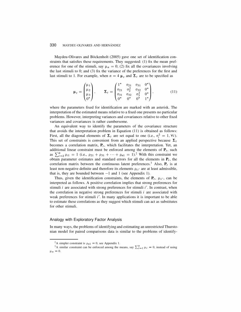
Consider a Thurstonian model for paired comparisons data where †t is sym-metric positive definite matrix. For n � 3, it follows from Tsai (2003) that nC2
constraints must be introduced to identify this model. Because of the compara-tive nature of the data, one constraint needs to be imposed among the elementsof �t . Also, n constraints need to be imposed on the elements of †t such thatone constraint is imposed among the elements in each of the rows (columns) ofthis matrix. These location constraints are needed because A is of rank n � 1.An additional constraint must be introduced among the elements of †t to setthe scale for the remaining parameters.
330 MAYDEU-OLIVARES AND HERNÁNDEZ
Maydeu-Olivares and Böckenholt (2005) gave one set of identification con-straints that satisfies these requirements. They suggested: (1) fix the mean pref-erence for one of the stimuli, say �n D 0; (2) fix all the covariances involvingthe last stimuli to 0; and (3) fix the variance of the preferences for the first andlast stimuli to 1. For example, when n D 4 �t and †t are to be specified as
�t D
0
B
B
@
�1
�2
�3
0�
1
C
C
A
; †t D
0
B
B
@
1� ¢21 ¢31 0�
¢21 ¢22 ¢32 0�
¢31 ¢32 ¢23 0�
0� 0� 0� 1�
1
C
C
A
; (11)
where the parameters fixed for identification are marked with an asterisk. Theinterpretation of the estimated means relative to a fixed one presents no particularproblems. However, interpreting variances and covariances relative to other fixedvariances and covariances is rather cumbersome.
An equivalent way to identify the parameters of the covariance structurethat avoids the interpretation problem in Equation (11) is obtained as follows:First, all the diagonal elements of †t are set equal to one (i.e., ¢2
i D 1; 8i ).This set of constraints is convenient from an applied perspective because †t
becomes a correlation matrix, Pt , which facilitates the interpretation. Yet, anadditional linear constraint must be enforced among the elements of Pt , suchas
PniD2 ¡i1 D 1 (i.e., ¡21 C ¡31 C � � � C ¡n1 D 1).2 With this constraint we
obtain parameter estimates and standard errors for all the elements in Pt , thecorrelation matrix between the continuous latent preferences.3 Also, Pt is atleast non-negative definite and therefore its elements ¡i i 0 are at least admissible,that is, they are bounded between �1 and 1 (see Appendix 1).
Thus, given the identification constraints, the elements of Pt , ¡i i 0 , can beinterpreted as follows. A positive correlation implies that strong preferences forstimuli i are associated with strong preferences for stimuli i 0. In contrast, whenthe correlation in negative strong preferences for stimuli i are associated withweak preferences for stimuli i 0. In many applications it is important to be ableto estimate these correlations as they suggest which stimuli can act as substitutesfor other stimuli.
Analogy with Exploratory Factor Analysis
In many ways, the problems of identifying and estimating an unrestricted Thursto-nian model for paired comparisons data is similar to the problems of identify-
2A simpler constraint is ¡n1 D 0, see Appendix 1.3A similar constraint can be enforced among the means, say
P
n
iD1 �i D 0, instead of using�n D 0.

ESTIMATION OF THURSTONE’S MODEL 331
ing and estimating an unrestricted factor model for binary data with n factors,where n is the number of stimuli being compared. Thus, in the Thurstonianunrestricted model (a) the contrast matrix A is analogous to the factor loadingsmatrix, (b) the means of the continuous latent preferences �t . are analogousto the factor means, (c) the matrix of correlations among the preferences Pt isanalogous to the matrix of inter-factor correlations, and (d) the diagonal ma-trix �2 containing the variances of the pair specific errors is analogous to thediagonal matrix containing the variances of the unique factors.
The easiest way to obtain a set of identified parameters in an unrestrictedfactor model is to (a) set the factors to be uncorrelated, and (b) set the uppertriangular part of the factor loading matrix equal to zero (McDonald, 1999:p. 181). The factor means are not identified in an unrestricted factor model andthey are set to zero. In an unrestricted Thurstonian model the ‘factor means’ �t .can be estimated because the ‘factor loadings matrix’ A is a matrix of contrast.To identify the Thurstonian model, we fix one of the ‘factor means’ to zero, andwe impose a linear constraint among the ‘inter-factor correlations’.
For an unrestricted factor model with estimated matrices of factor loadingsƒ and inter-factor correlations ˆ, it is well known that alternative solutionswith Qƒ and Q that yield an equivalent fit can be obtained by rotating the axes.Analogously, for an unrestricted Thurstonian model with estimated matrices ofpreferences means �t , preferences intercorrelations Pt , and pair specific errorvariances �2, applied researchers can obtain alternative solutions that yield an
equivalent fit with matrices Q�t , QPt , and Q�2using the equation
Q�t Dp
c�t ;QPt D cPt C .1 � c/110; Q�2 D c�2; (12)
where c is any positive constant such that QPt is a correlation matrix (i.e., it isnon-negative definite). This is proved in Appendix 2.
Thus, just as when fitting an unrestricted factor analysis, the applied re-searcher that fits an unrestricted Thurstonian model must bear in mind that thesolution obtained is not the only one that is consistent with the data. Other so-lutions exist that will yield the same fit to the data. For the unrestricted factormodel, applied researchers often use rotation algorithms (e.g., Varimax, Oblimin)to aid explore alternative solutions that may be more consistent with substan-tive theory. Exploring alternative solutions that may be more consistent withsubstantive theory is easier for the unrestricted Thurstonian model as appliedresearchers just need to plug in different values of c in Equation (12). How-ever, even though this equation plays the same role as factor rotation in factoranalysis, it is not a rotation. Also, just as in factor analysis it is possible toincorporate any substantive knowledge into the model and resort to confirma-tory factor analysis, in Thurstonian modeling the applied researcher may wishto incorporate any substantive knowledge into the model, and estimate a model
332 MAYDEU-OLIVARES AND HERNÁNDEZ
where some elements of the parameter matrices �t , Pt , and �2 are fixed at apriori values, or where some parameters are set equal to other parameters in themodel.
SEM ESTIMATION OF THURSTONIAN MODELS FOR
PAIRED COMPARISONS DATA
Among the most popular statistical packages for structural equation modeling,EQS (Bentler, 2004), Lisrel (Jöreskog & Sörbom, 2001) and Mplus (Muthén &Muthén, 2001) implement multistage procedures for estimating structural equa-tion models with binary dependent variables. In these methods, first the thresh-olds and tetrachoric correlations are estimated from the univariate and bivariatemargins of the contingency table. In a second stage, the structural parametersare estimated from the estimated thresholds and tetrachoric correlations. In thissection, the estimation of Thurstonian models for paired comparisons data isdescribed.
Let pk and pkk0 be the sample counterpart of k D Pr.yk D 1/ and kk0 DPr.yk D 1; yk0 D 1/, respectively, and let ˆn.�/ denote a n-variate standardnormal distribution function. Then, first each element of £ is estimated separatelyusing O£k D �ˆ�1
1 .pk/. Next, each tetrachoric correlation is estimated separatelygiven the first stage estimates using O¡kk0 D ˆ�1
2 .pkk0 j �O£k; �O£k0/. This methodfor estimating the tetrachoric correlations is equivalent to those implemented inLisrel and Mplus, but not in EQS.
Then, letting › D .£0; ¡0/0, the model parameters ™ are estimated by mini-mizing
F D . O› � ›.™//0 OW. O› � ›.™// (13)
where OW D O„�1(weighted least squares, WLS: Muthén, 1978), OW D .Diag
. O„//�1 (diagonally weighted least squares, DWLS: Muthén, du Toit, & Spisic,1997), or OW D I (unweighted least squares, ULS: Muthén, 1993), and „ denotesthe asymptotic covariance (Acov) matrix of
pN . O› � ›/.
Standard errors for the parameter estimates are obtained using Acov. O™/ D1N
H„H0, where H D .�0W�/�1�0W, and � D @›@™0 (Muthén, 1993). WLS
estimation is known to perform poorly in small samples (Muthén, 1993). Also,ULS performs better than DWLS estimation in small samples (Maydeu-Olivares,2001). Thus, in this paper ULS will be employed.
Goodness of fit tests of the restrictions imposed by the model on the thresh-olds and tetrachoric correlations for the DWLS and ULS estimators can beobtained (Muthén, 1993; Satorra & Bentler, 1994) by scaling T WD N OF by itsmean or adjusting it by its mean and variance so that it approximates a chi-square
ESTIMATION OF THURSTONE’S MODEL 333
distribution using Ts D rTrŒM�
T , and Ta D TrŒM�
TrŒM2�T , where M D W.I � �H/„.
Ts and Ta, denote the scaled (for mean) and adjusted (for mean and variance) teststatistics. Ts is referred to a chi-square distribution with r D Qn. QnC1/
2� q degrees
of freedom, where q is the number of mathematically independent parameters
in ™. Ta is referred to a chi-square distribution with d D .TrŒM�/2
TrŒM2�degrees of
freedom.It is important to bear in mind, however, that these test statistics do not assess
how well the model reproduces the data. Rather, they assess how well the modelreproduces the estimated thresholds and tetrachoric correlations. These statisticsare computed under a dichotomized multivariate normality assumption. Muthénand Hofacker (1988) proposed a test of dichotomized normality for triplets ofvariables. However, this test is not implemented in Mplus, Lisrel, nor EQS. Mostimportantly, it is not clear what to conclude if the assumption of dichotomizednormality is tenable for some triplets of variables, but not for all of them. Ratherthan testing separately the dichotomized multivariate normality underlying theuse of tetrachoric correlations, and testing the structural restrictions imposed bythe model on the tetrachoric correlations, Maydeu-Olivares (2001) proposed atest of the overall restrictions (structural and distributional) imposed by a SEMmodel on the dichotomous data. Let p be the Qn. QnC1/
2vector of first and second
order proportions, and let be its corresponding probabilities. Furthermore, let.p � . O™// be the vector of residual univariate and bivariate proportions underthe model. Then, goodness of fit tests of the overall restrictions imposed by themodel on the first and second order marginals of the contingency table .™/
can be obtained by scaling QT D N.p � . O™//0.p � . O™// using QTs D r
TrŒ QM�QT ,
and QTa D TrŒ QM�
TrŒ QM2�QT , where QM D .I � Q��H Q��1
/�.I � Q��H Q��1/0, � denotes
the asymptotic covariance matrix ofp
N .p � /, and Q� D @ @›0
. QTs and QTa are
to be referred to a chi-square distribution with r and d D .TrŒ QM�/2
TrŒ QM2�degrees of
freedom, respectively. A small simulation study reported in Maydeu-Olivares(2001) revealed that for some models the mean and variance adjusted statisticyields accurate Type I error rates in models with 21 variables with as few as100 observations.
AN APPLICATION: MODELING PREFERENCES
FOR CELEBRITIES
Kroeger (1992) replicated a classical experiment by Rumelhart and Greeno(1971) in which college students were presented with pairs of celebrities and theywere asked to select the celebrity with whom they would rather spend an hour ofconversation. Here we shall analyze a subset of Kroeger’s data consisting of the

334 MAYDEU-OLIVARES AND HERNÁNDEZ
females’ responses (96 subjects) to the paired comparisons involving the set offormer U.S. first ladies (Barbara Bush, Nancy Reagan, and Hillary Clinton) andathletes (Bonnie Blair, Jackee Joyner-Kersee, and Jennifer Capriati). Becauseno prior knowledge is available, we shall estimate an unrestricted Thurstonianmodel.
When a single population is involved, Mplus but not current versions4 ofLisrel and EQS can estimate single population models for categorical dependentvariables with mean or threshold structures (as required for Thurstonian model-ing of paired comparisons). Consequently, Mplus will be used in this example.The Mplus input file used in this example is provided in Appendix 3.
Fitting an Unrestricted Thurstonian Model
Estimating a Thurstonian unrestricted model for paired comparisons data is sim-ilar to estimating a factor model for binary data with n factors, where n is thenumber of stimuli being compared. Thus, to estimate the Thurstonian unre-stricted model the factor loadings must be fixed constants, those of the contrastmatrix A. Also, the factor means are estimated. This is mean vector of the stimulipreferences �t . Finally, the variances of the unique factors are estimated. Thisis the diagonal matrix �2 containing the variances of the pair specific errors.To identify the model, one of the factor means is fixed to zero. Also, the factorvariances are fixed to 1, so that the correlations among the preferences for thestimuli are estimated. This is the matrix Pt . Finally, a linear constraint needsto be imposed among the inter-factor correlations. See Appendix 3 for detailson how to implement this constraint in Mplus. For this example, we fixed themean of the last stimuli to zero, and imposed the constraint that the inter-factorcorrelations involving the first stimuli added to one.
For ULS estimation, only the mean and variance corrected statistic for testingthe restrictions imposed by the model on the thresholds and tetrachoric corre-lations is available in Mplus. We obtained Ta D 43:28 on 32 df,5 p D 0:09.It appears as if the structural restrictions imposed by this model be reasonable.However, an improper solution is obtained as the estimates for two of the di-agonal elements of �2 are negative. This is most likely due to the sample sizebeing too small to estimate this model.
As an alternative, we considered a model where the variances of the pairspecific errors are equal for all pairs, �2 D ¨2I. This restriction constraints
4At the time of this writing, the current versions of Mplus, Lisrel and EQS are 3.12, 8.7, and6.1, respectively.
5When mean and variance corrections are used, the number of degrees of freedom is estimated.This is a real number, which in Mplus is rounded to the nearest integer. For this model, the differencebetween the number of simple statistics and the number of estimated parameters is 86. This is highlyconstrained model.
ESTIMATION OF THURSTONE’S MODEL 335
the expected number of intransitivities to be approximately equal for all pairs(Maydeu-Olivares & Böckenholt, 2005). For this model, which has 14 parame-ters less than the previous model, we obtained Ta D 44:57 on 33 df, p D 0:09.Also, the estimate of the common variance of the pair specific errors is a propervalue, 0.24. The more restricted model is clearly to be preferred. Finally, usingthe test statistic proposed by Maydeu-Olivares (2001) evaluated at the Mplusestimates for this model we can also assess whether the model reproducesthe data. We obtained QTs D 124:62 on 100 df, p D 0:05, and QTa D 20:05
on 16.09 df, p D 0:22. The model reproduces well the paired comparisonspatterns.
The estimates and standard errors for the parameters of this model are shownin Table 1. Taking into account the estimated standard errors, the ordering ofthe mean preferences for these celebrities under this model is {Hillary Clinton,Jackee Joyner D Barbara Bush D Jennifer Capriati, and Bonnie Blair D NancyReagan}. Yet, preferences for the most preferred celebrity, Hillary Clinton, arenot significantly correlated with preferences for any other celebrity. On the otherhand, preferences for Bonnie Blair are significantly and positively related topreferences for all the other celebrities (but Hillary Clinton). In addition, womenthat express their preference for Barbara Bush are significantly more likely toprefer Jennifer Capriati as well.
TABLE 1
Parameter Estimates and Standard Errors for an Unrestricted Covariance Structure Model
Assuming �2 D ¨2I Applied to the Celebrities Data
P t
Barbara
Bush
Nancy
Reagan
Hillary
Clinton
Bonnie
Blair
Jackee
Joyner
Jennifer
Capriati
Barbara Bush 1(fixed)
Nancy Reagan 0.74 1(0.09) (fixed)
Hillary Clinton �0.22 �0.37 1(0.24) (0.29) (fixed)
Bonnie Blair 0.24 0.35 �0.19 1(0.12) (0.14) (0.28) (fixed)
Jackee Joyner �0.01 0.04 �0.47 0.37 1(0.16) (0.18) (0.32) (0.16) (fixed)
Jennifer Capriati 0.26 0.21 �0.56 0.44 0.32 1(0.13) (0.19) (0.33) (0.15) (0.20) (fixed)
�t 0.09 �0.28 0.43 �0.27 0.16 0(0.15) (0.15) (0.20) (0.13) (0.14) (fixed)
N D 96; ¡21 C ¡31 C � � � C ¡n1 D 1; standard errors in parentheses; correlations in bold aresignificant at ’ D 0:05; O2 D 0:26 (0.06).
336 MAYDEU-OLIVARES AND HERNÁNDEZ
Transformation of the Solution
Just as an unrestricted factor model can be rotated to explore alternative solutionsthat may be more consistent with substantive theory, the unrestricted Thurstonianmodel can be transformed to explore alternative solutions that may be moreconsistent with substantive theory. To transform the solution shown in Table 1we just need to search through the set of solutions given in Equation (12). In thisexample, we believe that stronger preferences for Hillary Clinton are associatedwith weaker preferences for Nancy Reagan. Consequently we shall transformthe solution to achieve the maximum negative correlation between these twostimuli. Assigning values greater than 1 to c in Equation (12) the correlationbetween Nancy Reagan and Hillary Clinton becomes increasingly negative. Themaximum value that c can take in this application resulting in a positive definitetransformed QPt is 1.10. When c takes this value, the correlation between thepreferences for Nancy Reagan and Hillary Clinton becomes �0.51, this is thelargest negative correlation for these two stimuli that results in a proper model.Now, we can obtain standard errors for this transformed solution by simply re-estimating the model using the code given in Appendix 3 where the constraintPn
iD2 ¡i1 D 1 used to obtain the initial solution is replaced by the constraintcorr(Nancy Reagan, Hillary Clinton) D �0.51. The results of this transformedsolution are given in Table 2. This solution yields the same goodness of fit asthe solution presented in Table 1, but is slightly easier to interpret. Accordingto the solution, for this population of female college students the most preferredcelebrity to spend an hour of conversation with is Hillary Clinton (as it hasthe highest mean preference). The least preferred ones are Bonnie Blair andNancy Reagan. Mean preferences for the remaining celebrities are roughly equaland in between these extremes. We also observe two significant associations inTable 2. Students who prefer to spend an hour of conversation with NancyReagan as more likely to prefer an hour of conversation with Barbara Bush,and students who prefer to spend an hour with Hillary Clinton are less likely toprefer spending an hour with Jennifer Capriati.
Accuracy of the Results
The small sample size (96) relative to the number of binary paired comparisonsmodeled (15) casts doubts on the reliability of these results. The Monte Carlo ca-pabilities of Mplus can be used to address this concern since a simulation studycan be performed using as true parameter values the estimated parameters of themodel. Using the Mplus input file provided in Appendix 4, we performed a sim-ulation study to investigate the accuracy of the parameter estimates, standard er-rors, and goodness of fit tests obtained in our initial model where
PniD2 ¡i1 D 1.
The simulation of 1000 samples of size 96 took 56 seconds on a 3 Mz machine.

ESTIMATION OF THURSTONE’S MODEL 337
TABLE 2
Estimated Parameter and Standard Errors for the Transformed Solution
P t
Barbara
Bush
Nancy
Reagan
Hillary
Clinton
Bonnie
Blair
Jackee
Joyner
Jennifer
Capriati
Barbara Bush 1(fixed)
Nancy Reagan 0.71 1(0.11) (fixed)
Hillary Clinton �0.35 �0.51 1(0.18) (fixed) (fixed)
Bonnie Blair 0.16 0.28 �0.19 1(0.26) (0.22) (0.28) (fixed)
Jackee Joyner �0.12 �0.05 �0.62 0.31 1(0.36) (0.31) (0.38) (0.25) (fixed)
Jennifer Capriati 0.18 0.13 �0.72 0.38 0.25 1(0.27) (0.39) (0.33) (0.21) (0.30) (fixed)
�t 0.09 �0.29 0.46 �0.28 0.17 0(0.15) (0.16) (0.21) (0.15) (0.15) (fixed)
The solution was transformed so that the correlation between preferences for Nancy Reaganand Hillary Clinton was maximally negative; standard errors in parentheses; correlations in bold aresignificant at ’ D 0:05; O2 D 0:28 (0.09).
All replications converged. The bias of the parameter estimates, x O™� ™0, ranged
from �0.02 to 0.01 with an average of 0. The bias of the standard errors,x
SE.O™/� sdO™
, ranged from �0.01 to 0.01, with an average of 0. The coverageof the 95% confidence intervals for the parameter estimates ranged from 0.92to 0.96, with an average or 0.94. Clearly, the parameter estimates and standarderrors we have obtained in our small sample application are to be trusted. As forthe behavior of the test statistic implemented in Mplus, the empirical rejectionrates at ’ D f0:01; 0:05; 0:10; 0:20g across the 1000 replications were {0.01,0.03, 0.09, 0.18}. The p-values yielded by the test statistic are reliable. Themodel indeed reproduces the estimated thresholds and tetrachoric correlations.
DISCUSSION AND CONCLUSIONS
Maydeu-Olivares and Böckenholt (2005) have recently shown how to embed theclass of Thurstonian models for paired comparison data within a SEM frame-work. They also provide details on how to estimate these models using Mplus.Yet, the comparative nature of paired comparisons data causes problems ofparameter interpretation in these models. For the Case V, Case III, as wellas Thurstonian factor analytic models Maydeu-Olivares and Böckenholt (2005)

338 MAYDEU-OLIVARES AND HERNÁNDEZ
show how to suitably identify these models to obtain interpretable parameters.Yet, the interpretation of the parameters of the unrestricted Thurstonian modelproved difficult. This model plays a crucial role in Thurstonian modeling, asit is the most general model within this class. In this paper, we have extendedMaydeu-Olivares and Böckenholt (2005) results by providing a set of identifica-tion restrictions for this model that yield an easily interpretable solution. Thus,we have shown that the correlations among the continuous latent preferencescan be estimated, if one constraint is imposed among them. With this constraint,the correlation matrix of the CLPs is at least non-negative definitive. Given theclose connection between Thurstonian models for paired comparisons and rank-ing data (see Maydeu-Olivares and Böckenholt, 2005), this specification of theunrestricted Thurstonian model can also be applied to ranking data.
The solution obtained is not the only one that is consistent with the data.Alternative solutions can be obtained by transforming the solution initially ob-tained that yield an equivalent fit to the data. A formula has been provided thatenables searching for alternative solutions that may be more consistent withsubstantive theory.
Also, we have shown in this paper how applied researchers can use Mplus’simulation capabilities to investigate the accuracy of the parameter estimates,standard errors, and goodness of fit tests obtained using this program for theirparticular application. Unfortunately, researchers can currently test with Mplusonly the restrictions imposed by their structural models on the estimated thresh-olds and tetrachoric correlations. This test need not be meaningful if the as-sumption of categorized normality does not hold. It is possible to test the over-all restrictions imposed by Thurstonian models on the observed binary data(Maydeu-Olivares, 2001) and existing evidence suggest that these tests performas well as the structural restrictions tests in small samples. However, the testsof the overall restrictions are yet to be implemented in Mplus.
To sum up, framing the analysis of paired comparisons data within a structuralequation modeling framework enables applied researchers to conveniently andreliably estimate and test the full array of Thurstonian models. It is hoped thatthe widespread availability of software to estimate structural equation modelingwill encourage further use of these experimental designs in applications.
ACKNOWLEDGMENTS
The authors are very much indebted to the reviewers for comments that ledto substantial improvements to the manuscript. This research was supported bythe Dept. of Universities, Research and Information Society (DURSI) of theCatalan Government, and by grants BSO2000-0661 and BSO2003-08507 fromthe Spanish Ministry of Science and Technology.

ESTIMATION OF THURSTONE’S MODEL 339
REFERENCES
Bentler, P. M. (2004). EQS. Encino, CA: Multivariate Software Inc.Bock, R. D., & Jones, L. V. (1968). The measurement and prediction of judgment and choice. San
Francisco: Holden-Day.Böckenholt, U. (2001a). Hierarchical modeling of paired comparison data. Psychological Methods,
6, 49–66.Böckenholt, U. (2001b). Thresholds and intransitivities in pairwise judgments: A multilevel analysis.
Journal of Educational and Behavioral Statistics, 26, 269–282.Böckenholt, U. (2004). Comparative judgments as an alternative to ratings: Identifying the scale
origin. Psychological Methods, 4, 453–465.Böckenholt, U., & Dillon, W. R. (1997). Modeling within-subject dependencies in ordinal paired
comparison data. Psychometrika, 62, 411–434.Böckenholt, U., & Tsai, R. C. (2001). Individual differences in paired comparison data. British
Journal of Mathematical and Statistical Psychology, 54, 265–277.Dudgeon, P., Bell, R., & Pattison, P. (2003). Imposing constraints on Cholesky-decomposed co-
variance matrices. Paper presented at the International Meeting of the Psychometric Society,Cagliari.
Jöreskog, K.G., & Sörbom, D. (2001). LISREL 8. Chicago, IL: Scientific Software.Kroeger, K. (1992). Unpublished dataset. University of Illinois, Urbana-Champaign.Maydeu-Olivares, A. (1999). Thurstonian modeling of ranking data via mean and covariance struc-
ture analysis. Psychometrika, 64, 325–340.Maydeu-Olivares, A. (2001). Limited information estimation and testing of Thurstonian models for
paired comparison data under multiple judgment sampling. Psychometrika, 66, 209–228.Maydeu-Olivares, A. (2002). Limited information estimation and testing of Thurstonian models for
preference data. Mathematical Social Sciences, 43, 467–483.Maydeu-Olivares, A. (2003). On Thurstone’s model for paired comparisons and ranking data. In
H. Yanai, A. Okada, K. Shigematu, Y. Kano, & J. J. Meulman (Eds.), New developments in
psychometrics (pp. 519–526). Tokyo: Springer.Maydeu-Olivares, A. (2004). Thurstone’s Case V model: A structural equation modeling perspective.
In K. van Monfort, J. Oud, & A. Satorra (Eds.), Recent developments on structural equation
models (pp. 41–67). Dordrecht: Kluwer.Maydeu-Olivares, A., & Böckenholt, U. (2005). Structural equation modeling of paired comparison
and ranking data. Psychological Methods, 10, 285–304.McDonald, R. P. (1999). Test theory. A unified approach. Mahwah, NJ: Lawrence Erlbaum.Muthén, B. (1978). Contributions to factor analysis of dichotomous variables. Psychometrika, 43,
551–560.Muthén, B. (1993). Goodness of fit with categorical and other non normal variables. In K. A. Bollen
& J. S. Long (Eds.), Testing structural equation models (pp. 205–234). Newbury Park, CA: Sage.Muthén, B., du Toit, S. H. C., & Spisic, D. (1997). Robust inference using weighted least squares
and quadratic estimating equations in latent variable modeling with categorical and continuousoutcomes. Unpublished manuscript. College of Education, UCLA. Los Angeles, CA.
Muthén, B., & Hofacker, C. (1988). Testing the assumptions underlying tetrachoric correlations.Psychometrika, 53, 563–578.
Muthén, L., & Muthén, B. (2001). MPLUS. Los Angeles, CA: Muthén & Muthén.Rummelhart, D. L., & Greeno, J. G. (1971). Similarity between stimuli: An experimental test of the
Luce and Restle choice models. Journal of Mathematical Psychology, 8, 370–381.Satorra, A., & Bentler, P. M. (1994). Corrections to test statistics and standard errors in covariance
structure analysis. In A. von Eye, & C. C. Clogg (Eds.), Latent variable analysis: Applications
to developmental research (pp. 399–419). Thousand Oaks, CA: Sage.

340 MAYDEU-OLIVARES AND HERNÁNDEZ
Searle, S. R. (1982). Matrix algebra useful for statistics. New York: Wiley.Steiger, J. H. (2002). When constraints interact: A caution about reference variables, identification
constraints, and scale dependencies in structural equation modeling. Psychological Methods, 7,210–227.
Takane, Y. (1987). Analysis of covariance structures and probabilistic binary choice data. Commu-
nication and Cognition, 20, 45–62.Tsai, R. C. (2000). Remarks on the identifiability of Thurstonian ranking models: Case V, Case III,
or neither? Psychometrika, 65, 233–240.Tsai, R. C. (2003). Remarks on the identifiability of Thurstonian paired comparison models under
multiple judgment. Psychometrika, 68, 361–372.Tsai, R. C., & Böckenholt, U. (2001). Maximum likelihood estimation of factor and ideal point
models for paired comparison data. Journal of Mathematical Psychology, 45, 795–811.Tsai, R. C., & Böckenholt, U. (2002). Two-level linear paired comparison models: Estimation and
identifiability issues. Mathematical Social Sciences, 43, 429–449.Tsai, R. C., & Wu, T. L. (2004). Analysis of paired comparison data using Mx. Structural Equation
Modeling: An Interdisciplinary Journal, 11, 73–91.Thurstone, L. L. (1927). A law of comparative judgment. Psychological Review, 79, 281–299.
APPENDIX 1
Identification of the Unrestricted Thurstonian Model
To identify †t Maydeu-Olivares and Böckenholt (2005) used the following n
constraints ¢n1 D 0; : : : ; ¢n;n�1 D 0, ¢nn D 1. In contrast, here we use the n
constraints ¢i i D 1; 8i so that a correlation matrix Pt is estimated. Letting ¡i i 0 bean element of Pt and ¢i i 0 be a parameter in Maydeu-Olivares and Böckenholt’s†t , the relationship between both parameterizations is
¡i i 0 D
8
ˆ
ˆ
ˆ
<
ˆ
ˆ
ˆ
:
1 � ¢i 0i 0
2if i D n
2 C 2¢i i 0 � ¢i i � ¢i 0i 0
2otherwise
: (14)
The inverse relationship is
¢i i 0 D
8
<
:
2 � ¡ni 0 if i D i 0
¡i i 0 � ¡ni � ¡ni 0 otherwise: (15)
To show that Pt is indeed a correlation matrix, notice that we can decomposeit using a Cholesky decomposition as Pt D CC0, where C is a lower triangularmatrix whose diagonal elements are constrained such that Pt has ones along itsdiagonal. Dudgeon, Bell and Pattison (2003) have recently provided details on
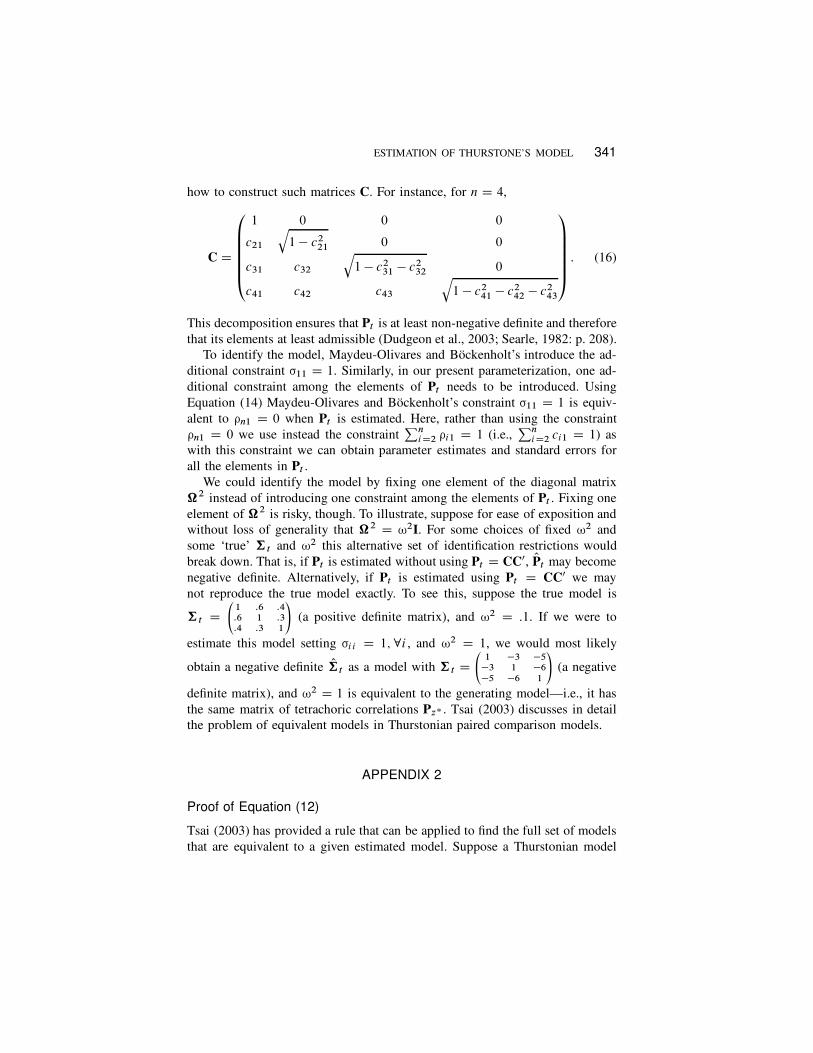
ESTIMATION OF THURSTONE’S MODEL 341
how to construct such matrices C. For instance, for n D 4,
C D
0
B
B
B
B
B
@
1 0 0 0
c21
q
1 � c221 0 0
c31 c32
q
1 � c231 � c2
32 0
c41 c42 c43
q
1 � c241 � c2
42 � c243
1
C
C
C
C
C
A
: (16)
This decomposition ensures that Pt is at least non-negative definite and thereforethat its elements at least admissible (Dudgeon et al., 2003; Searle, 1982: p. 208).
To identify the model, Maydeu-Olivares and Böckenholt’s introduce the ad-ditional constraint ¢11 D 1. Similarly, in our present parameterization, one ad-ditional constraint among the elements of Pt needs to be introduced. UsingEquation (14) Maydeu-Olivares and Böckenholt’s constraint ¢11 D 1 is equiv-alent to ¡n1 D 0 when Pt is estimated. Here, rather than using the constraint¡n1 D 0 we use instead the constraint
PniD2 ¡i1 D 1 (i.e.,
PniD2 ci1 D 1) as
with this constraint we can obtain parameter estimates and standard errors forall the elements in Pt .
We could identify the model by fixing one element of the diagonal matrix�2 instead of introducing one constraint among the elements of Pt . Fixing oneelement of �2 is risky, though. To illustrate, suppose for ease of exposition andwithout loss of generality that �2 D ¨2I. For some choices of fixed ¨2 andsome ‘true’ †t and ¨2 this alternative set of identification restrictions wouldbreak down. That is, if Pt is estimated without using Pt D CC0, OPt may becomenegative definite. Alternatively, if Pt is estimated using Pt D CC0 we maynot reproduce the true model exactly. To see this, suppose the true model is
†t D0
@
1 :6 :4:6 1 :3:4 :3 1
1
A (a positive definite matrix), and ¨2 D :1. If we were to
estimate this model setting ¢i i D 1; 8i , and ¨2 D 1, we would most likely
obtain a negative definite O†t as a model with †t D0
@
1 �3 �5�3 1 �6�5 �6 1
1
A (a negative
definite matrix), and ¨2 D 1 is equivalent to the generating model—i.e., it hasthe same matrix of tetrachoric correlations Pz� . Tsai (2003) discusses in detailthe problem of equivalent models in Thurstonian paired comparison models.
APPENDIX 2
Proof of Equation (12)
Tsai (2003) has provided a rule that can be applied to find the full set of modelsthat are equivalent to a given estimated model. Suppose a Thurstonian model

342 MAYDEU-OLIVARES AND HERNÁNDEZ
for paired comparisons has been estimated. For this specific model, we denotethe covariance matrix of the continuous latent preferences as †t and the errorcovariance matrix as �2. Both matrices must be positive definite. Then, any
other model with †2 and Q�2of the form
Q†t D c†t C d10 C 1d0; and Q�2 D c�2; (17)
is equivalent to the estimated model (Tsai, 2003; Corollary 1). That is, it yieldsthe same fit to the data. In Equation (17) c is a positive constant and d is an
n � 1 vector of constants. These constants are arbitrary as long as Q†t and Q�2
are positive definite.Here, the estimated model is a correlation matrix, that is, †t D Pt , and we
use (17) to find the set of alternative correlation matrices QPt that are equallyconsistent with the data. Thus, we write
QPt D cPt C d10 C 1d0; and Q�2 D c�2: (18)
The first of these equations yields for the diagonal elements the relationship1 D c C 2di ) di D 1�c
2, i D 1; : : : ; n. That is, for (18) to hold d D .1�c
2/1.
Substituting into Equation (18) we obtain QPt D cPt C .1�c2
/110 C .1�c2
/110 DcPt C .1 � c/110.
The relationship among the mean vectors can be obtained as follows. Againfrom Tsai (2003, section 4), two equivalent models should also satisfy
QDt A Q�t D DtA�t (19)
where A is the design matrix and D D .Diag.APt A0 C �2//� 12 , QD D .Diag
.A QPt A0 C Q�2//� 1
2 . From QPt D cPt C .1 � c/110 it is then easy to verify that
QD D .Diag.A QPt A0 C Q�2//� 1
2 D .Diag.c.APt A0 C �2///� 12 D 1p
cD
and so
QDA Q�t D DA�t ) Dt A Q�t D Dt A.p
c�t/ ) A Q�t D A.p
c�t /
If we fix the last component of the mean vector to 0, this implies Q�t Dpc�t as requested.

ESTIMATION OF THURSTONE’S MODEL 343
APPENDIX 3
Mplus Input File for Modeling the Preferences for
Celebrities
TITLE: ULS estimation for first ladies and sportwomen
(females resp only);
DATA: FILE IS ‘ladies sport.dat’;
! the data contains 96 observations on 15 binary variables
VARIABLE:
NAMES ARE
y12 y13 y14 y15 y16
y23 y24 y25 y26
y34 y35 y36
y45 y46
y56;
! it is convenient to assign names that reflect the paired
comparisons
CATEGORICAL = y12-y56;
! variables are declared as categorical
ANALYSIS:
TYPE = MEANSTRUCTURE;
! thresholds and tetrachoric correlations are modeled
ESTIMATOR = ULS;
! ULS estimation, mean and variance corrected test
statistic
PARAMETERIZATION = THETA;
! it enables modeling factor variances with categorical
dependent vars
MODEL:
f1 BY y12-y16@1;
f2 by y23-y26@1;
f3 by y34-y36@1;
f4 BY y45-y46@1;
f5 by y56-y56@1;

344 MAYDEU-OLIVARES AND HERNÁNDEZ
f2 by y12@-1;
f3 by y13@-1 y23@-1;
f4 by y14@-1 y24@-1 y34@-1;
f5 by y15@-1 y25@-1 y35@-1 y45@-1;
f6 by y16@-1 y26@-1 y36@-1 y46@-1 y56@-1;
! fixed factor loadings, this is the A matrix
! the factors are
! f1 = Barbara Bush
! f2 = Nancy Reagan
! f3 = Hillary Clinton
! f4 = Bonnie Blair
! f5 = Jackee Joyner
! f6 = Jennifer Capriati
[y12$1-y56$1@0];
! thresholds fixed to zero
[f1-f5* f6@0];
! factor means free --default is fixed to zero
y12-y56*.2(1);
! error specific variances equal
! for this matrix to be diagonal use instead
! y12-y56*.2;
f1-f6@1;
! factor variances are fixed at 1
f2 with f3-f6;
f3 with f4-f6;
f4 with f6*;
f5 with f6*;
! all factors are intercorrelated
f1 with f2* (p1);
f1 with f3* (p2);
f1 with f4* (p3);
f1 with f5* (p4);
f1 with f6 (p5);
! factor intercorrelations with first stimuli

ESTIMATION OF THURSTONE’S MODEL 345
MODEL CONSTRAINT:
p5 = 1 - p1 - p2 - p3 -p4;
! enforces constraint that the sum of factor
! inter-correlations with first stimuli = 1
OUTPUT: TECH1;
! use this to verify that the A matrix is properly set up
SAVEDATA: ESTIMATES=estimates.dat;
! save estimates for Monte Carlos simulation
APPENDIX 4
Mplus Input File for Monte Carlo Simulation
TITLE: simulation for first ladies and sportwomen data,
ULS estimation;
MONTECARLO:
NAMES ARE y12 y13 y14 y15 y16 y23 y24 y25 y26 y34 y35
y36 y45 y46 y56 ;
NOBS=96;
! same sample size as in the application is used
NREPS = 1000;
! 1000 replications are requested
SEED = 4553;
GENERATE = y12-y56(1);
! multivariate normal data is generated
! each variable is categorized using one threshold
CATEGORICAL = y12-y56;
! the data is analyzed as categorical
POPULATION = estimates.dat;
COVERAGE = estimates.dat;
! the estimated parameter values from the application
! are used as true parameter values to generate the data
MODEL POPULATION:
! same model as in the application
f1 BY y12-y16@1;
f2 by y23-y26@1;

346 MAYDEU-OLIVARES AND HERNÁNDEZ
f3 by y34-y36@1;
f4 BY y45-y46@1;
f5 by y56-y56@1;
f2 by y12@-1;
f3 by y13@-1 y23@-1;
f4 by y14@-1 y24@-1 y34@-1;
f5 by y15@-1 y25@-1 y35@-1 y45@-1;
f6 by y16@-1 y26@-1 y36@-1 y46@-1 y56@-1;
f1-f6@1;
[y12$1-y56$1@0];
[f1-f5* f6@0];
y12-y56*.2(1);
f1 with f2-f6*;
f2 with f3-f6*;
f3 with f4-f6*;
f4 with f5-f6*;
f5 with f6*;
! the inter-factor correlation matrix is left unconstrained
ANALYSIS:
TYPE = MEANSTRUCTURE;
ESTIMATOR = ULS;
! ULS estimation, mean and variance corrected test statistic
PARAMETERIZATION = THETA;
MODEL:
! same model as in the application
f1 BY y12-y16@1;
f2 by y23-y26@1;
f3 by y34-y36@1;
f4 BY y45-y46@1;
f5 by y56-y56@1;
f2 by y12@-1;
f3 by y13@-1 y23@-1;
f4 by y14@-1 y24@-1 y34@-1;
f5 by y15@-1 y25@-1 y35@-1 y45@-1;
f6 by y16@-1 y26@-1 y36@-1 y46@-1 y56@-1;

ESTIMATION OF THURSTONE’S MODEL 347
f1-f6@1;
[y12$1-y56$1@0];
[f1-f5* f6@0];
y12-y56*.2(1);
f2 with f3-f6;
f3 with f4-f6;
f4 with f6*;
f5 with f6*;
f1 with f2* (p1);
f1 with f3* (p2);
f1 with f4* (p3);
f1 with f5* (p4);
f1 with f6 (p5);
MODEL CONSTRAINT:
p5 = 1 - p1 - p2 - p3 -p4;