Identifiability of stiffness components of clear wood from a

single off-axes compression test

J. Xaviera, A. Majano-Majanob, Jose Fernandez-Cabob

aCITAB, UTAD, Engenharias I, Apartado 1013, 5001-801 Vila Real, PortugalbETS of Architecture, Structural Department, Technical University of Madrid (UPM), Madrid,

Spain

Abstract

In this work, the identifiability of orthotropic stiffness components of clear woodfrom a single off-axis compression test was investigated. The parameter identifica-tion strategy was based on anisotropic elasticity theory, so-called anisotropic-basedmethod. The proposed approach couples off-axes compression tests on prismaticspecimens with 3D full-field measurements. In practice, these measurements canbe provided by a suitable optical technique such as stereovision or ESPI. Exper-imentally, specific tests were carried out in order to deal with boundary issuessuch as friction and shear-extension coupling effects. Numerically, a finite elementmodel of the mechanical test was built as a support for optimal inspection the testconfiguration in terms of angles orientation (direction cosine matrix), such thatbalanced strain components can be reached in the material coordinate system.Results, conclusions and future work were discussed in view of the identifiabilityof all active stiffness components from only one test configuration.

Keywords: Wood, Digital image correlation, material parameter identification,Compression tests

1. Introduction

The parameters governing constitutive equations of materials are determinedexperimentally by means of suitable mechanical tests. In the field of solid mechan-ics, this issue is presented as an inverse problem where the material parametersare to be determined from the knowledge of geometry, boundary conditions andstrains (or displacements). Conventionally, this identification is achieved by car-rying out mechanical tests in which specimen geometry and loading system aredesigned to generate homogeneous or simple strain/stress states across the gaugeregion. The underlying idea behind this assumption is useful for theoretical analy-ses because closed-form solutions can be obtained, relating the unknown materialparameters to the load and strain measurements (statically determined tests).

July 26, 2012

However, the practical implementation of these tests can be difficult, especially foranisotropic and heterogeneous materials such as wood. The recent developmentof full-field optical techniques has enabled a new glance on the mechanical testsfor material characterisation. The basic idea driving this new approach is that asingle specimen can be loaded in order that several parameters are involved in themechanical response, yielding heterogeneous and complex strain fields (staticallyundetermined tests). By means of a suitable identification strategy all the activeparameters can be determined afterwards.

Wood is a biological composite material formed by trees. It can be analysedat several scales of observation from timber down to chemical constituents. Themechanisms of deformation in wood can be quite complex involving, for instance,anisotropic, viscoelastic and hygroscopic phenomena. Moreover, the intra and in-ter variability of wood is reflected on the material parameters governing relevantconstitutive equations. Therefore, the investigation of the wood mechanical be-haviour raises several difficulties from both modelling and experimental points ofview. In most practical applications and with some simplification hypothesis, in-voking low levels of stress, short periods of time and minor variations of moisturecontent and temperature, wood can be modelled as a linear elastic anisotropicmaterial. Besides, at the macro scale (0.1-1 m) wood is usually assumed as acontinuum and homogeneous medium. The complete characterisation of the lin-ear elastic orthotropic behaviour of clear wood requires the determination of nineindependent stiffness components. Conventionally, this set of material parametersare determined experimentally by carrying out several test methods, in which bothloading and specimen geometry are usually oriented along the material directions.Moreover, these tests are based on the assumption of simple and homogeneousstress/strain states across the elementary representative volume of the material atthe scale of observation. This approach represents a great effort from an exper-imental point of view because only a few (i.e., one or two) stiffness componentsare obtained per test configuration. Besides, the complete stiffness matrix willbe characterised from different test and specimen configurations, enhancing vari-ability. In order to overcome these limitations, a single off-axes compression testmethod for clear wood has been recently proposed [1]. This project aims furtherimprovements of the test method with regard to the identifiability of the wholeset of orthotropic stiffness components. Both experimental and numerical analysiswill be addressed. 3D full-field measurements provided by a stereovision and EPSIwill be envisaged. Preliminary tests were carried out in order to deal with bound-ary issues such as friction and shear-extension coupling effects, coupling off-axescompression tests with stereosivion technique (ARAMISr system by GOM). Nu-merically, finite element analyses of the mechanical test method were performedin order to optimise the test configuration in terms of angles orientation (direction

2

cosine matrix), such that balanced strain components are reached in the materialcoordinate system.

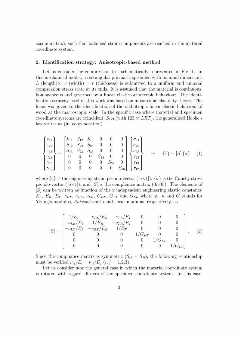
2. Identification strategy: Anisotropic-based method

Let us consider the compression test schematically represented in Fig. 1. Inthis mechanical model, a rectangular prismatic specimen with nominal dimensionsL (length)× w (width) × t (thickness) is submitted to a uniform and uniaxialcompression stress state at its ends. It is assumed that the material is continuous,homogeneous and governed by a linear elastic orthotropic behaviour. The identi-fication strategy used in this work was based on anisotropic elasticity theory. Thefocus was given to the identification of the orthotropic linear elastic behaviour ofwood at the macroscopic scale. In the specific case where material and specimencoordinate systems are coincident, S123 (with 123 ≡ LRT ), the generalised Hooke’slaw writes as (in Voigt notation)

ε11ε22ε33γ23γ13γ12

=

S11 S12 S13 0 0 0S12 S22 S23 0 0 0S13 S23 S33 0 0 00 0 0 S44 0 00 0 0 0 S55 00 0 0 0 0 S66

σ11

σ22

σ33

τ23τ13τ12

⇒ {ε} = [S] {σ} (1)

where {ε} is the engineering strain pseudo-vector ([6×1]), {σ} is the Cauchy stresspseudo-vector ([6×1]), and [S] is the compliance matrix ([6×6]). The elements of[S] can be written as function of the 9 independent engineering elastic constants:EL, ER, ET , νRT , νLT , νLR, GRT , GLT and GLR where E, ν and G stands forYoung’s modulus, Poisson’s ratio and shear modulus, respectively, as

[S] =

1/EL −νRL/ER −νTL/ET 0 0 0

−νLR/EL 1/ER −νTR/ET 0 0 0−νLT/EL −νRT/ER 1/ET 0 0 0

0 0 0 1/GRT 0 00 0 0 0 1/GLT 00 0 0 0 0 1/GLR

. (2)

Since the compliance matrix is symmetric (Sij = Sji), the following relationshipmust be verified νij/Ei = νji/Ej (i, j = 1,2,3).

Let us consider now the general case in which the material coordinate systemis rotated with regard all axes of the specimen coordinate system. In this case,

3

Figure 1: Schematic representation of the off-axis compression test.

the stress state in the material coordinate system ([σ]) can be determined fromthe applied stress state in the specimen coordinate system ([σ′]) by the followingtransformation rule of second-order symmetric tensors

[σ] = [T ]T [σ′][T ], (3a)

with

[σ] =

σ11 σ12 σ13

σ12 σ22 σ23

σ13 σ23 σ33

, [σ′] =

σxx σxy σxz

σxy σyy σyz

σxz σyz σzz

and [T ] =

l1 l2 l3m1 m2 m3

n1 n2 n3

(3b)

where σij = τij when i ̸= j, [T ]T is the transpose of matrix [T ] and lk, mk e nk

(k = 1, 2, 3) are the direction cosine between material and specimen coordinatesystems. In Voigt notation, Eq. (3) writes

σ11

σ22

σ23

τ23τ13τ12

=

l 21 m 2

1 n 21 2l1m1 2m1n1 2l1n1

l 22 m 22 n 2

2 2l2m2 2m2n2 2l2n2

l 23 m 23 n 2

3 2l3m3 2m3n3 2l3n3

l1l2 m1m2 n1n2 l1m2 + l2m1 m1n2 +m2n1 l1n2 + l2n1

l2l3 m2m3 n2n3 l2m3 + l3m2 m2n3 +m3n2 l2n3 + l3n2

l1l3 m1m3 n1n3 l1m3 + l3m1 m1n3 +m3n1 l1n3 + l3n1

σxx

σyy

σzz

τyzτxzτxy

(4a)

or{σ} = [Tσ′σ] {σ′} . (4b)

4

In the same way, the strain tensor in the material and specimen coordinate systemare transformed by the following rule

[ε] = [T ]T [ε′][T ], (5a)

with

[ε] =

ε11 ε12 ε13ε12 ε22 ε23ε13 ε23 ε33

and [ε′] =

εxx εxy εxzεxy εyy εyzεxz εyz εzz

(5b)

where εij = γij/2 when i ̸= j. In Voigt notation, Eq. (5) writes

ε11ε22ε23γ23γ13γ12

=

l 21 m 2

1 n 21 l1m1 m1n1 l1n1

l 22 m 22 n 2

2 l2m2 m2n2 l2n2

l 23 m 23 n 2

3 l3m3 m3n3 l3n3

2l1l2 2m1m2 2n1n2 l1m2 + l2m1 m1n2 +m2n1 l1n2 + l2n1

2l2l3 2m2m3 2n2n3 l2m3 + l3m2 m2n3 +m3n2 l2n3 + l3n2

2l1l3 2m1m3 2n1n3 l1m3 + l3m1 m1n3 +m3n1 l1n3 + l3n1

εxxεyyεzzγyzγxzγxy

(6a)

or{ε} = [Tε′ε] {ε′} . (6b)

The transformation matrices of stress ([Tσ′σ]) and strain ([Tε′ε]) satisfy the follow-ing properties

[Tσ′σ]−1 = [Tε′ε]

T and [Tε′ε]−1 = [Tσ′σ]

T . (7)

The transformation of the compliance matrix [S], between material and speci-men coordinate systems, can be deduced from the above Eqs (3-7). Starting fromEq. (1) one gets

{ε} = [S] {σ} ⇔ [Tε′ε] {ε′} = [S][Tσ′σ] {σ′} ⇔ {ε′} = [Tσ′σ]T [S][Tσ′σ] {σ′} . (8)

Therefore, in an arbitrary off-axes configuration, the Hooke’s law in the specimencoordinate system is given by

εxxεyyεzzγyzγxzγxy

=

S ′11 S ′

12 S ′13 S ′

14 S ′15 S ′

16

S ′12 S ′

22 S ′23 S ′

24 S ′25 S ′

26

S ′13 S ′

23 S ′33 S ′

34 S ′35 S ′

36

S ′14 S ′

24 S ′34 S ′

44 S ′45 S ′

46

S ′15 S ′

25 S ′35 S ′

45 S ′55 S ′

56

S ′16 S ′

26 S ′36 S ′

46 S ′56 S ′

66

σxx

σyy

σzz

τyzτxzτxy

⇒ {ε} = [S] {σ} (9)

5

with,[S ′] = [Tσ′σ]

T [S][Tσ′σ]. (10)

From the anisotropic elasticity theory, it is possible to derive an explicit rela-tionship linking unknown compliance coefficients with specimen dimensions, load-ing configuration and strain measurements as

[Tε′ε] {ε′} = [S][Tσ′σ] {σ′} (11)

in which,

- [Tε′ε] and [Tσ′σ]: are transformation matrices whose elements are cosine directionsdefined in function of the off-axis angles between material and specimencoordinates systems;

- {ε′}: lists the strain components across the gauge section in the specimen coor-dinate system;

- {σ′}: lists the stress state applied to the specimen (applied load).

- [S]: is a function of the components of the compliance matrix completely definingthe orthotropic behaviour of the material.

In practice, the strain components at the gauge section ({ε′}) can be determined bya suitable full-field optical method, as for instance, 3D digital image correlation.When the orthotropic material can be assumed homogeneous, an average valueover the gauge section can be determined.

Given an off-axes configuration, let us consider a first loading case consistingin a uniaxial compression stress along the x direction

{σx} ={F/A, 0, 0, 0, 0, 0

}T. (12)

In this case the linear system of Eqs. (11) can be re-written as

σxx

l21 l22 l23 0 0 0 0 0 00 l21 0 l22 l23 0 0 0 00 0 l21 0 l22 l23 0 0 00 0 0 0 0 0 l1l2 0 00 0 0 0 0 0 0 l2l3 00 0 0 0 0 0 0 0 l1l3

S11

S12

S13

S22

S23

S33

S44

S55

S66

= [Tε′ε] {ε′} (13a)

6

or, in compact form[Ax] {S} = {bx} (13b)

The system of Eqs. (13) is undetermined since there are only six equations for nineunknowns compliance elements. In order to solve this linear system, a possibilityis considering at least two independent loading cases. In practice, this can beachieved by carrying out the compression test along different loading axis, as forinstance,

• Uniaxial loading case 1:

{σx} = {F/A, 0, 0, 0, 0, 0}T =⇒ [Ax] {S} = {bx}

• Uniaxial loading case 2:

{σy} = {0, F/A, 0, 0, 0, 0}T =⇒ [Ay] {S} = {by}

• Uniaxial loading case 3:

{σz} = {0, 0, F/A, 0, 0, 0}T =⇒ [Az] {S} = {bz}This approach yields to an overdetermined system of equation which can be solvedwith regard to the compliance components ({S}) using the concept of pseudo-inverse. Generically, for the three compression loading systems, Eqs. (13) can bere-write as [Ax]

[Ay][Az]

{S} =

{bx}{by}{bz}

(14a)

or, in compact form[R] {S} = {q} . (14b)

Finally, Eqs. (14) can then be solved as

{S} = ([R]−1[R])−1[R]−1 {q} . (15)

3. Finite element analyses

3.1. Finite element model

A 3D finite element model of the off-axis compression test was built in ANSYSr

14. Clear wood was modelled as a continuous and homogeneous medium with anorthotropic linear elastic behaviour. Maritime pine (Pinus pinaster Ait.) was con-sidered with properties as summarised in Table 1 [2]. According to the experimen-tal work, the dimensions of the specimen were taken equal to 68(R)×36(T)×33(L)mm [1]. The 3D 8-node structural SOLID185 was selected from the element library.

7

Table 1: Engineering constants of maritime pine used in finite element analyses [2].

EL ER ET νRT νTL νLR GRT GLT GLR

(GPa) (GPa) (GPa) (-) (-) (-) (GPa) (GPa) (GPa)

15.1 1.91 1.01 0.59 0.051 0.47 0.286 1.22 1.41

The ANEL anisotropic elastic model was used for material parameter definition.A mesh with 37407 nodes and 34370 elements was defined (Fig. 2). The elementsize was set to 1.25 mm, which is an order of magnitude higher than the displace-ment spatial resolution that can be typically achieved experimentally by a digitalimage correlation technique. No symmetry of the model about the y and z axeswas taken into account, so the numerically deformation across the whole lateralsurfaces could be processed exactly as performed experimentally [1].

The compression test was simulated by contact boundary conditions. The com-pression plates were simulated by a rigid surface TARGE170 element. CONTA173element was selected for simulating the contact interface between bottom and topsurfaces of the model and the target rigid surface. Degree of freedom (translationsand rotations) were then applied to target nodes simulating the compression testin the linear elastic domain. The friction coefficient of 0.5 was firstly chosen, but itcan be changed according to the experimental procedure for reduction of frictioneffects.

The convergence of the model (mesh and contact boundary conditions) waschecked assuming a compression test parallel to the grain (i.e., in which materialand specimen coordinate systems were coincident) based on a specimen with nom-inal dimensions of 25(R)×25(T)×100(L) mm according to the ASTM D 143 stan-dard [3] (longitudinal direction L parallel to the y axis of the specimen). From thenumerical deformation at an external surface, a longitudinal modulus of elasticitywas determined according to the following closed-form solution (data reduction):EL = (P/A)/εL, where P represents the global applied load, A is the cross-sectionof the specimen and εL is the axial strain along the longitudinal direction. Numer-ically, P was determined as the vertical reaction force at the upper target nodes.Moreover, εL was defined as the average value of the nodal y axial strains withina central area of 5×5 mm (this area could correspond experimentally to the mea-suring region covered by a strain gauge or an optical method). The error betweenthe calculated and reference EL values was negligible.

3.2. Identifiability analyses

The finite element model presented before will be used in further analyses inorder to investigate boundary effects on the mechanical response of the specimen.Moreover, it will be used to optimise the test configuration in terms of grain

8

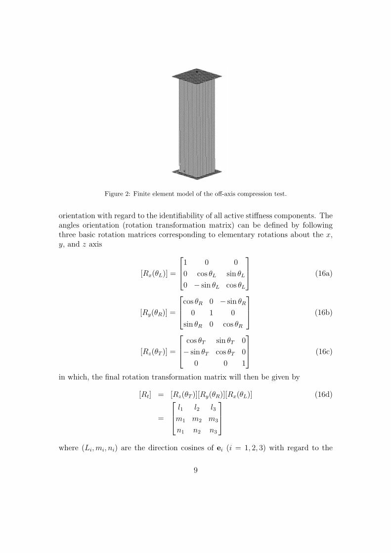
Figure 2: Finite element model of the off-axis compression test.

orientation with regard to the identifiability of all active stiffness components. Theangles orientation (rotation transformation matrix) can be defined by followingthree basic rotation matrices corresponding to elementary rotations about the x,y, and z axis

[Rx(θL)] =

1 0 0

0 cos θL sin θL

0 − sin θL cos θL

(16a)

[Ry(θR)] =

cos θR 0 − sin θR

0 1 0

sin θR 0 cos θR

(16b)

[Rz(θT )] =

cos θT sin θT 0

− sin θT cos θT 0

0 0 1

(16c)

in which, the final rotation transformation matrix will then be given by

[Rt] = [Rz(θT )][Ry(θR)][Rx(θL)] (16d)

=

l1 l2 l3

m1 m2 m3

n1 n2 n3

where (Li,mi, ni) are the direction cosines of ei (i = 1, 2, 3) with regard to the

9

global coordinate system S(0, i, j,k). For the purpose of optimum test configura-tion, a cost function can be defined as

ϕ(θL, θR, θT ) =△

6(ε21 + ε22 + ε23 + γ223 + γ2

13 + γ212)

. (17a)

with

△ = (ε1 − ε2)2 + (ε1 − ε3)

2 + (ε1 − γ23)2 + (ε1 − γ13)

2 + (ε1 − γ12)2 (17b)

+(ε2 − ε3)2 + (ε2 − γ23)

2 + (ε2 − γ13)2 + (ε2 − γ12)

2

+(ε3 − γ23)2 + (ε3 − γ13)

2 + (ε3 − γ12)2

+(γ23 − γ13)2 + (γ23 − γ12)

2 + (γ13 − γ12)2

Eventually, the minimisation of the cost function, ϕ(θi) (i = L,R, T ) (Eq. 17),should yield a configuration in which the strain components are balanced outand evenly spread across the gauge section. Therefore, this configuration shouldcorrespond to an optimum configuration for the multi-parameter identificationpurposes.

The strain components on the material coordinate system figuring in the costfunction of Eq. (17) can be deduced analytically from the anisotropic elasticitytheory. From this theory and assuming a uniaxial stress state along the x axis(σx = εx/S

′11) the following expression can be obtained

ε1/εx = (S11l21 + S12l

22 + S13l

23)/S

′11 (18a)

ε2/εx = (S12l21 + S22l

22 + S23l

23)/S

′11

ε3/εx = (S13l21 + S23l

22 + S33l

23)/S

′11

γ23/εx = (S44l1l2)/S′11

γ13/εx = (S55l2l3)/S′11

γ12/εx = (S66l1l3)/S′11

withS ′11 = S11c

4 − 2S16c3s+ (2S12 + S66)c

2s2 − 2S26cs3 + S22s

4 (18b)

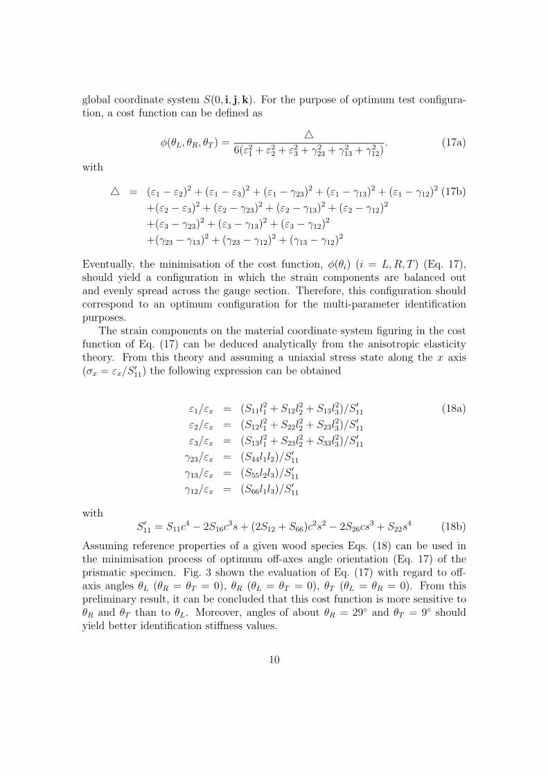
Assuming reference properties of a given wood species Eqs. (18) can be used inthe minimisation process of optimum off-axes angle orientation (Eq. 17) of theprismatic specimen. Fig. 3 shown the evaluation of Eq. (17) with regard to off-axis angles θL (θR = θT = 0), θR (θL = θT = 0), θT (θL = θR = 0). From thispreliminary result, it can be concluded that this cost function is more sensitive toθR and θT than to θL. Moreover, angles of about θR = 29◦ and θT = 9◦ shouldyield better identification stiffness values.

10

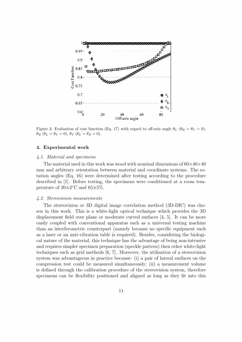
Figure 3: Evaluation of cost function (Eq. 17) with regard to off-axis angle θL (θR = θT = 0),θR (θL = θT = 0), θT (θL = θR = 0).

4. Experimental work

4.1. Material and specimens

The material used in this work was wood with nominal dimensions of 60×40×40mm and arbitrary orientation between material and coordinate systems. The ro-tation angles (Eq. 16) were determined after testing according to the proceduredescribed in [1]. Before testing, the specimens were conditioned at a room tem-perature of 20±2◦C and 65±5%.

4.2. Stereovision measurements

The stereovision or 3D digital image correlation method (3D-DIC) was cho-sen in this work. This is a white-light optical technique which provides the 3Ddisplacement field over plane or moderate curved surfaces [4, 5]. It can be moreeasily coupled with conventional apparatus such as a universal testing machinethan an interferometric counterpart (namely because no specific equipment suchas a laser or an anti-vibration table is required). Besides, considering the biologi-cal nature of the material, this technique has the advantage of being non-intrusiveand requires simpler specimen preparation (speckle pattern) then other white-lighttechniques such as grid methods [6, 7]. Moreover, the utilisation of a stereovisionsystem was advantageous in practice because: (i) a pair of lateral surfaces on thecompression test could be measured simultaneously; (ii) a measurement volumeis defined through the calibration procedure of the stereovision system, thereforespecimens can be flexibility positioned and aligned as long as they fit into this

11

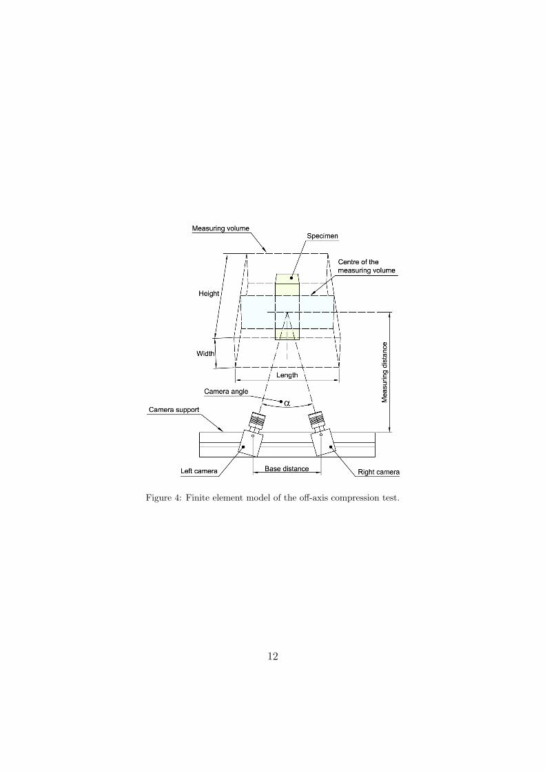
Figure 4: Finite element model of the off-axis compression test.

12

Figure 5: Finite element model of the off-axis compression test.

virtual space. However, when compared to a monovision system (DIC-2D), themain disadvantage is that the uncertainty on the evaluation of the parameters ofthe camera model represents an additional uncertainty on the displacement mea-surement, and therefore on the evaluation of the material parameters.

The stereovision technique is a full-field technique for measuring the 3D (in-plane and out-of-plane) displacement/strain fields of a given 3D object. The anal-ysis is based on a sequence of pair of stereo images recorded during the objectdeformation. A binocular stereovision (a measuring system with a pair of left andright cameras) is used for assessing the position of a 3D point in space (with regardto a given world coordinate system) from the knowledge of its stereo projectionpoints in the two recorded images (Fig. 4). This process is known as triangulation.On the one hand, this method requires a camera calibration consisting in determin-ing the extrinsic (the relative position and orientation of the coordinates systemsassociated to the two cameras) and intrinsic parameters of the camera model. Onthe other hand, a correspondence of the projection points on the two cameras mustbe established (stereo-matching problem) using for instance the epipolar constantconcept.

The digital image correlation method is based on the assumption that thesurface of the object under analysis has a textured pattern such that the lightintensity, diffusely reflected over the surface, will vary continuously with a suit-able contrast. Different techniques have been successfully used for the creation ofsuch a speckle pattern, employing spray or airbrush paint, toner powder depositor lithography. In this work, the speckle pattern was created by aerosol spray,applying a thin coating of white paint followed by a spot distribution of blackpaint (Fig. 5).

In the DIC method, the displacement field is measured by analysing the geo-metrical deformation of the images of the surface of interest, recorded before and

13

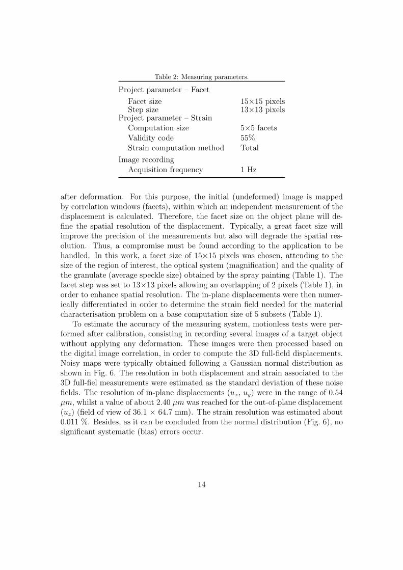
Table 2: Measuring parameters.

Project parameter – Facet

Facet size 15×15 pixelsStep size 13×13 pixels

Project parameter – StrainComputation size 5×5 facetsValidity code 55%Strain computation method Total

Image recordingAcquisition frequency 1 Hz

after deformation. For this purpose, the initial (undeformed) image is mappedby correlation windows (facets), within which an independent measurement of thedisplacement is calculated. Therefore, the facet size on the object plane will de-fine the spatial resolution of the displacement. Typically, a great facet size willimprove the precision of the measurements but also will degrade the spatial res-olution. Thus, a compromise must be found according to the application to behandled. In this work, a facet size of 15×15 pixels was chosen, attending to thesize of the region of interest, the optical system (magnification) and the quality ofthe granulate (average speckle size) obtained by the spray painting (Table 1). Thefacet step was set to 13×13 pixels allowing an overlapping of 2 pixels (Table 1), inorder to enhance spatial resolution. The in-plane displacements were then numer-ically differentiated in order to determine the strain field needed for the materialcharacterisation problem on a base computation size of 5 subsets (Table 1).

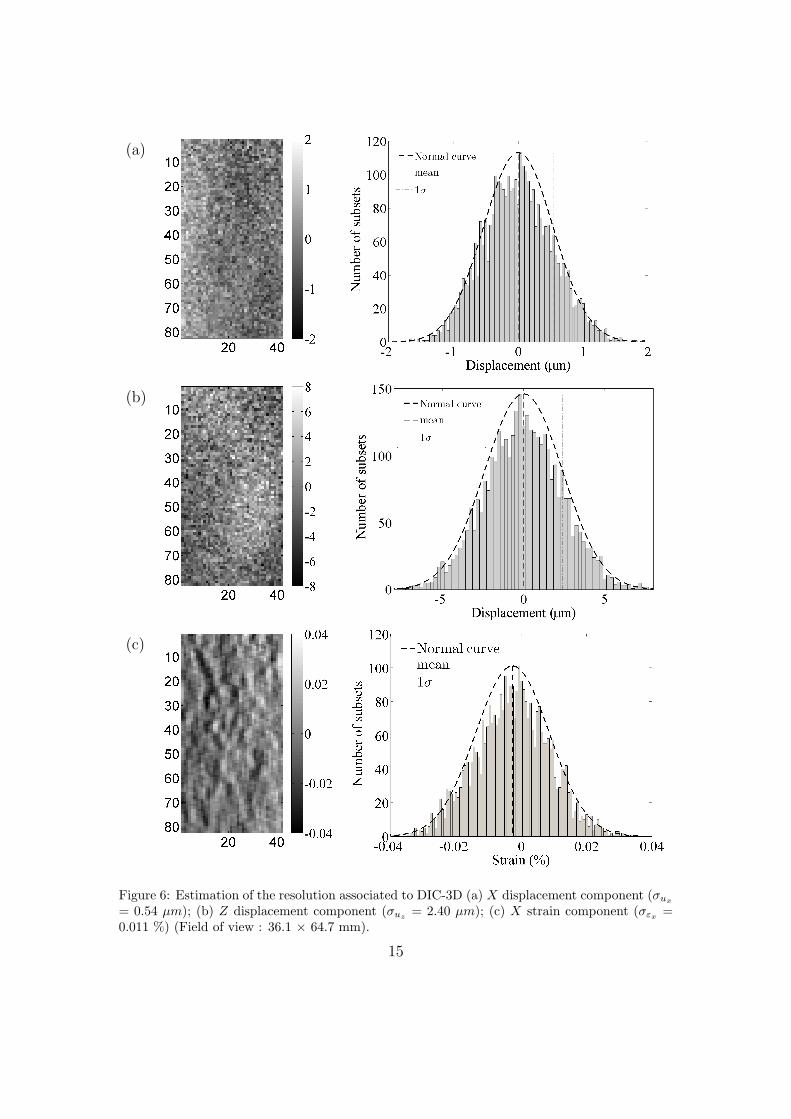
To estimate the accuracy of the measuring system, motionless tests were per-formed after calibration, consisting in recording several images of a target objectwithout applying any deformation. These images were then processed based onthe digital image correlation, in order to compute the 3D full-field displacements.Noisy maps were typically obtained following a Gaussian normal distribution asshown in Fig. 6. The resolution in both displacement and strain associated to the3D full-fiel measurements were estimated as the standard deviation of these noisefields. The resolution of in-plane displacements (ux, uy) were in the range of 0.54µm, whilst a value of about 2.40 µm was reached for the out-of-plane displacement(uz) (field of view of 36.1 × 64.7 mm). The strain resolution was estimated about0.011 %. Besides, as it can be concluded from the normal distribution (Fig. 6), nosignificant systematic (bias) errors occur.

14

(a)

(b)

(c)

Figure 6: Estimation of the resolution associated to DIC-3D (a) X displacement component (σux

= 0.54 µm); (b) Z displacement component (σuz = 2.40 µm); (c) X strain component (σεx =0.011 %) (Field of view : 36.1 × 64.7 mm).

15

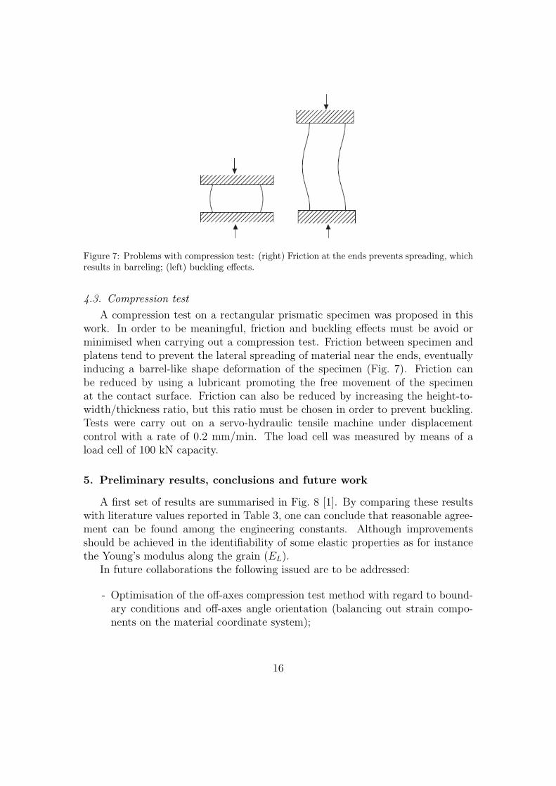
Figure 7: Problems with compression test: (right) Friction at the ends prevents spreading, whichresults in barreling; (left) buckling effects.

4.3. Compression test

A compression test on a rectangular prismatic specimen was proposed in thiswork. In order to be meaningful, friction and buckling effects must be avoid orminimised when carrying out a compression test. Friction between specimen andplatens tend to prevent the lateral spreading of material near the ends, eventuallyinducing a barrel-like shape deformation of the specimen (Fig. 7). Friction canbe reduced by using a lubricant promoting the free movement of the specimenat the contact surface. Friction can also be reduced by increasing the height-to-width/thickness ratio, but this ratio must be chosen in order to prevent buckling.Tests were carry out on a servo-hydraulic tensile machine under displacementcontrol with a rate of 0.2 mm/min. The load cell was measured by means of aload cell of 100 kN capacity.

5. Preliminary results, conclusions and future work

A first set of results are summarised in Fig. 8 [1]. By comparing these resultswith literature values reported in Table 3, one can conclude that reasonable agree-ment can be found among the engineering constants. Although improvementsshould be achieved in the identifiability of some elastic properties as for instancethe Young’s modulus along the grain (EL).

In future collaborations the following issued are to be addressed:

- Optimisation of the off-axes compression test method with regard to bound-ary conditions and off-axes angle orientation (balancing out strain compo-nents on the material coordinate system);

16

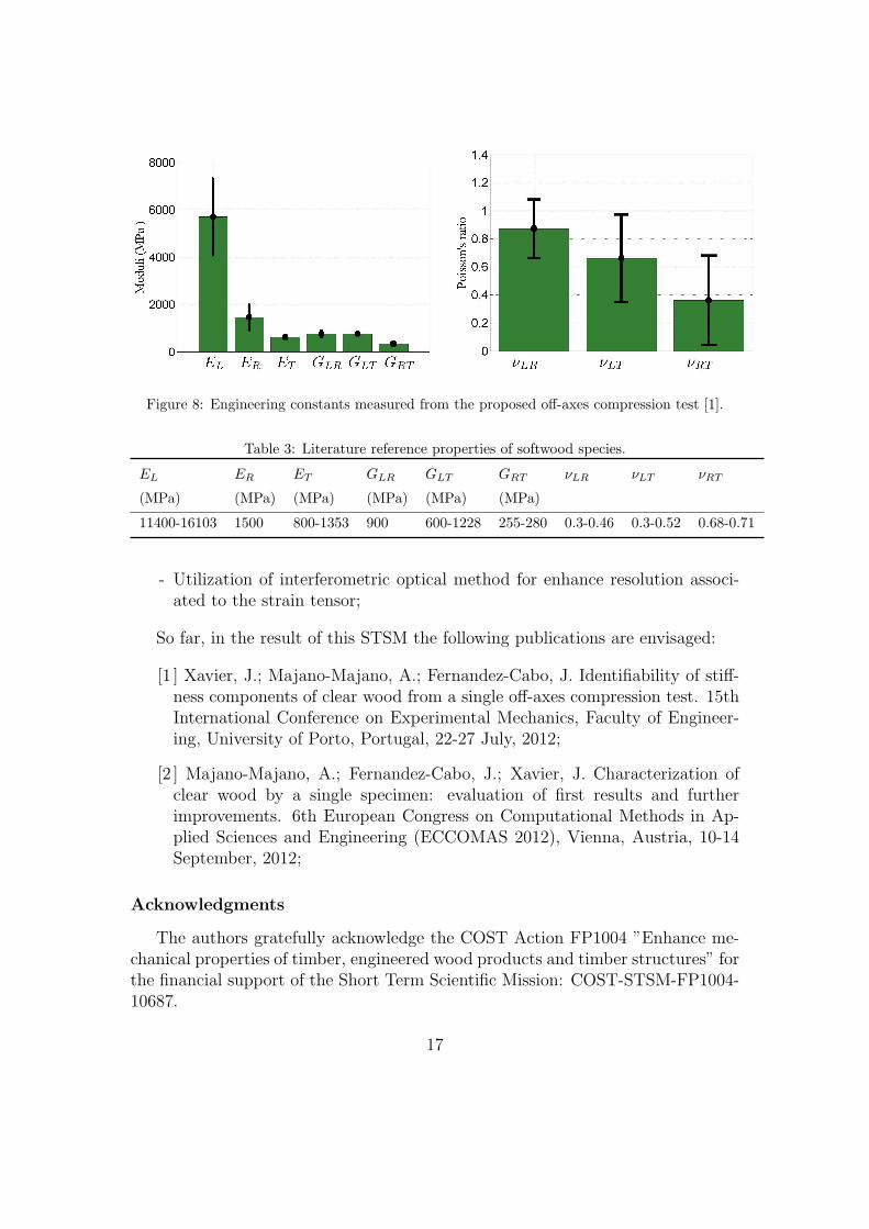
Figure 8: Engineering constants measured from the proposed off-axes compression test [1].

Table 3: Literature reference properties of softwood species.

EL ER ET GLR GLT GRT νLR νLT νRT

(MPa) (MPa) (MPa) (MPa) (MPa) (MPa)

11400-16103 1500 800-1353 900 600-1228 255-280 0.3-0.46 0.3-0.52 0.68-0.71

- Utilization of interferometric optical method for enhance resolution associ-ated to the strain tensor;

So far, in the result of this STSM the following publications are envisaged:

[1 ] Xavier, J.; Majano-Majano, A.; Fernandez-Cabo, J. Identifiability of stiff-ness components of clear wood from a single off-axes compression test. 15thInternational Conference on Experimental Mechanics, Faculty of Engineer-ing, University of Porto, Portugal, 22-27 July, 2012;

[2 ] Majano-Majano, A.; Fernandez-Cabo, J.; Xavier, J. Characterization ofclear wood by a single specimen: evaluation of first results and furtherimprovements. 6th European Congress on Computational Methods in Ap-plied Sciences and Engineering (ECCOMAS 2012), Vienna, Austria, 10-14September, 2012;

Acknowledgments

The authors gratefully acknowledge the COST Action FP1004 ”Enhance me-chanical properties of timber, engineered wood products and timber structures” forthe financial support of the Short Term Scientific Mission: COST-STSM-FP1004-10687.

17

References

[1] A. Majano-Majano, J. Fernandez-Cabo, S. Hoheisel, M. Klein, A test methodfor characterizing clear wood using a single specimen, Experimental Mechanics1 (1) (2012) 1–18.

[2] J. Xavier, N. Garrido, J. Oliveira, J. Morais, P. Camanho, F. Pierron, A com-parison between the Iosipescu and off-axis shear test methods for the char-acterization of pinus pinaster Ait., Composites Part A: Applied Science andManufacturing 35 (7-8) (2004) 827–840.

[3] ASTM D143, Standard methods of testing small clear specimens of timber,ASTM International, West Conshohocken, PA, 2007.

[4] J.-J. Orteu, 3-D computer vision in experimental mechanics, Optics and Lasersin Engineering 47 (3-4) (2009) 282–291.

[5] M. Sutton, J.-J. Orteu, H. Schreier, Image correlation for shape, motion anddeformation measurements: Basic concepts, theory and applications, Springer,2009.

[6] J. Xavier, S. Avril, F. Pierron, J. Morais, Novel experimental approach forlongitudinal-radial stiffness characterisation of clear wood by a single test,Holzforschung 61 (5) (2007) 573–581.

[7] J. Xavier, S. Avril, F. Pierron, J. Morais, Variation of transverse and shearstiffness properties of wood in a tree, Composites Part A: Applied Science andManufacturing 40 (2009) 1953–1960.

18