
Ict and Non-Ict Investments
30
LLEE Working Paper Series ICT AND NON-ICT INVESTMENTS: SHORT AND LONG RUN MACRO DYNAMICS Fabio Bacchini Maria Elena Bontempi Roberto Golinelli Cecilia Jona Lasinio Working Paper No. 113 July 2014 Luiss Lab of European Economics Department of Economics and Business LUISS Guido Carli Viale Romania 32, 00197, Rome -- Italy http://dptea.luiss.edu/research-centers/luiss-lab-european-economics © Fabio Bacchini Maria Elena Bontempi Roberto Golinelli Cecilia Jona Lasinio. The aim of the series is to diffuse the research conducted by Luiss Lab Fellows. The series accepts external contributions whose topics is related to the research fields of the Center. The views expressed in the articles are those of the authors and cannot be attributed to Luiss Lab.
Transcript of Ict and Non-Ict Investments
LLEE Working Paper Series
ICT AND NON-ICT INVESTMENTS:
SHORT AND LONG RUN MACRO DYNAMICS
Fabio Bacchini Maria Elena Bontempi Roberto Golinelli Cecilia Jona Lasinio Working Paper No. 113
July 2014
Luiss Lab of European Economics
Department of Economics and Business
LUISS Guido Carli Viale Romania 32, 00197, Rome -- Italy
http://dptea.luiss.edu/research-centers/luiss-lab-european-economics
© Fabio Bacchini Maria Elena Bontempi Roberto Golinelli Cecilia Jona Lasinio. The aim
of the series is to diffuse the research conducted by Luiss Lab Fellows. The series accepts external contributions whose topics is related to the research fields of the Center. The
views expressed in the articles are those of the authors and cannot be attributed to Luiss
Lab.
1
ICT and Non-ICT investments:
short and long run macro dynamics
Fabio Bacchini*, Maria Elena Bontempi
***, Roberto Golinelli
***, Cecilia Jona Lasinio
**
July 2014
Abstract
In this paper, we model business investment distinguishing between ICT (communication
equipment, hardware and software) and Non-ICT (machinery and equipment, and non-
residential buildings) components and taking into account asset specific characteristics
potentially affecting the reactivity of capital accumulation over the business cycle.
Business investment and ICT and Non-ICT assets are estimated within a VECM model to test,
in a unique framework, the assumptions of the flexible accelerator model (Clark, 1944, and
Koyck, 1954) and of the neoclassical model of Hall and Jorgenson (1967), as well as how
financial constraints and uncertainty influence investment behaviour (Hall and Lerner, 2010,
and Bloom, 2007).
Our findings suggest that the long-run relationship with standard macro determinants (output
and user cost) is verified for aggregate business capital stock as well as for individual Non-ICT
assets but not for ICT. In the short run, liquidity is a key determinant of investment behaviour
independently of the asset type. In the long-run, uncertainty significantly affects ICT. Finally,
the results of the counterfactual exercises over the latest Italian recession support the idea that
ICT is a key policy variable to foster the economic recovery.
JEL Classification: C52, C53, E22, E50
Keywords: Evaluation of Macro models, ICT Investments, Uncertainty, Liquidity constraints, .
(*) Econometric Studies and Economic Forecasting Division, Italian Institute of Statistics, ISTAT, Rome.
(**
) Econometric Studies and Economic Forecasting Division, Italian Institute of Statistics, ISTAT and LUISS
Lab of European Economics, Rome
(***
) Department of Economics, University of Bologna, Italy. Corresponding author: [email protected]
2
1. Introduction1
Since the seminal work of Clark (1917) up to the most recent contributions of Gaiotti (2013) and
Bachmann et al. (2013), the macro and micro economic literature have tried to identify the main factors
influencing capital accumulation given its prominent role in boosting economic growth.
Aggregate demand and consequently short term growth are reduced by low investment that in turn
negatively affects medium term growth via its impact on capital stock. In a recent analysis by Buti and Mohl
(2014) it is shown that investment is definitely the main driver of the growth differential between the
Eurozone and the US accounting for 20% and 21% of real GDP respectively. They estimate that a 5
percentage point reduction in the investment rate leads to a reduction of potential growth of around 0.5%. As
a consequence, the design of policy measures to foster the most reactive components of aggregate investment
turns out to be especially important in times of economic crisis.
Nevertheless, today there is still a weak empirical support for an inclusive macro or micro theoretical
model able to provide effective policy suggestions to stimulate heterogeneous investment expenditures. At
the macro level, especially, little is known about the determinants of asset specific business investment such
as Information and Communication Technologies (ICT) as compared to other non-technological assets
(machinery and equipment and non-residential buildings). Particularly, there is relatively limited work on
modelling ICT investment (De Arcangelis et al.,2004; and Guerrieri et al, 2011). But the increased economic
relevance of innovation and digitalization as major drivers of sustainable economic growth makes the
understanding of short and long run determinants of ICT investment a strategic policy issue. Moreover
modelling asset specific investment dynamics is even more relevant for policy purposes since ICT and
physical capital are driven by different forces. Firm level empirical analysis reveals that both ICT and
physical capital investment are strongly demand-driven, but ICT investment adjusts more rapidly to a given
demand shock. Further, ICT capital is characterized by above normal returns: evidence for European
countries shows that a 10% increase in ICT capital is related with a 0.23% increase in firm’s productivity
(Van Reenen et al, 2010). This suggests that programmes stimulating ICT investment may be beneficial for
counter-cyclical policies.
In this paper, we model aggregate level as well as ICT and Non-ICT investments adopting a macro
perspective. We test the empirical performance of structural investment models in a Vector Error Correction
Model (VECM)2 where we jointly evaluate the assumptions of the flexible accelerator model (Clark, 1944,
and Koyck, 1954), and of the neoclassical model of Hall and Jorgenson (1967), as well as the role of
financial constraints and uncertainty (Hall and Lerner, 2010, and Bloom, 2007) in determining investment
1 Paper presented at the DIW Macroeconometric Workshop 2013, Berlin, November 29-30. We are grateful to Giuseppe
De Arcangelis, Adrian Pagan, Carmine Pappalardo, Francesco Zollino, and to participants of the workshop and of
seminars in ISTAT for suggestions; the usual disclaimers apply.
2 The VECM approach is a strategy to develop VAR-based structural models for policy purposes on the basis of their
ability of accounting for the features and regularities of time series data (Qin, 2011).
3
behaviour. We also check for the existence of complementary effects between different types of investments.
To our knowledge, this paper offers an original contribution to the macroeconomic modelling of investment
as well as to the ICT literature adopting a novel approach to model ICT and Non-ICT investment behaviour.
In the analysis, we make two core assumptions: the actual capital stock is dynamically related with
the determinants of the desired stock (Caballero, 1999); and ICT and non-ICT capital may incur in different
adjustment costs thus responding differently to macroeconomic shocks. The second hypothesis is based on
the findings by Bloom (2007) suggesting that investment in knowledge capital (R&D) typically incurs flow
adjustment costs, while investment in physical capital usually deserves stock adjustment costs, thus implying
a different dynamics under uncertainty.
We test our approach on Italian business investment and capital stock by asset over the period 1980-
2012. Our empirical results support the assumption that ICT and Non-ICT respond differently to
macroeconomic fluctuations and that both aggregate business capital stock and its Non-ICT components
(machinery and equipment, and non-residential) are cointegrated. But, we do not find any evidence of a long
run relationship for ICT capital stock nor for any of its main components (communication equipment,
hardware and software). This finding, coupled with the evidence of the existence of a cointegration
relationship for ICT investment and its components, reinforces the hypothesis that ICT, as other knowledge
based assets (R&D), incurs in flow adjustment costs consistently with the evidence in Bloom(2007).3
Particularly, we find that the flexible neoclassical model can explain the long-run dynamics of Non-
ICT capital, while ICT investment flows are driven by liquidity constraints, uncertainty and R&D.
Interestingly, financial constraints are a key determinant for short run investment decisions independently of
the asset characteristics. The same holds for output in the long run.
Finally, we perform a counterfactual exercise in the framework of the Macroeconometric model of
the Italian statistical institute (MeMo-It) to test our approach on the Italian data in 2008-2013. The analysis
suggests the following: a lower level of uncertainty and better financial conditions could have accounted for
a cumulate increase of nearly 5% in total business investment with respect to its level in 2013, and 1.2% in
capital stock, thus increasing the GDP by 0.4%. ICT investment is the main driver of this result.
The paper is structured as follows. Section 2 surveys the basics of the macro and micro theoretical
and empirical literature on investment models. Section 3 illustrates our model and empirical strategy, and
section 4 shows our empirical results. Section 5 is focused on policy implications while section 6 concludes.
2. Modelling investment expenditure: macro and micro findings
Very few studies have analysed ICT investment determinants and most of them focused on factors
influencing ICT adoption in small and medium enterprises (Consoli, 2012). Traditionally, ICT capital
accumulation has been widely investigated in the economic growth literature to clarify its impact on
3 Few papers have tried to assess the complementarity between ICT and R&D with opposite results (Van Leeuwen et al.
2009, Cerquera and Klein, 2008).
4
productivity growth (Jorgenson and Stiroh, 1999; Jorgenson, 2001). More recently, O’Mahony and Vecchi
(2005) and Venturini (2009) look at the long-run relationship between ICT capital and output growth, using
panel cointegration techniques but with the goal of quantifying the impact of ICT capital accumulation on
productivity growth.
The accelerator model of Clark (1917) and the neoclassical intertemporal optimisation model of
Jorgenson (1963) have been the benchmark models to explain aggregate investment behaviour.
Investment decisions have short- and long-run characteristics that have to be taken into account
when modelling investment behaviour (Bernanke, 1983). Generally, macro theoretical models assume a long
run perspective focusing on the idea that an investment occurs when expected returns over the life of the
project exceed its costs (Hall and Jorgenson, 1967; Eisner, 1967; Tobin and Brainard, 1977).
The macro structural models were empirically tested since the beginning of the 1970s. Clark (1979)
provided an extensive analysis of the output-based and security-value models using U.S. macro data. He
found that a good explanation of factors influencing investment in machinery and equipment can be obtained
adopting the accelerator model. Few years later Gordon and Veitch (1986) went back to the standard
approach to estimate structural investment equations demonstrating that since economic aggregates play
multiple roles in explaining investment behaviour it is possible only to estimate reduced form equations
(Chirinko, 1983).
The modest empirical performance of macroeconomic models and the need to analyze investment
properties at higher frequencies determined a shift from macro to micro data analysis (Caballero, 1999).
However, as largely demonstrated, the most popular empirical implementation, the q-model of Brainard and
Tobin (1968), and Tobin (1969), has a low performance since it produces estimated coefficients for the Q
variable (the measured shadow value of capital) which imply unrealistically high marginal adjustment costs
and therefore implausibly slow adjustment speeds (Whited, 1994). The q-model is seriously misspecified
because it does not allow for market imperfections (Hubbard, 1998), non-convex adjustment costs
(Caballero, 1999), and fixed adjustment costs and irreversibility (Bertola and Caballero, 1994, Caballero et
al., 1995, and Cooper and Haltiwanger, 2006) which may differently affect individual capital inputs and be
more relevant for intangibles than for tangibles, or for buildings than for equipment.4 So, aggregation of
capital inputs fails to consider that capital is heterogeneous and that firms use many types of capital assets in
the production process. The assumption of capital homogeneity might be responsible also for the poor
empirical performance of the neoclassical inter-temporal optimization investment model (Chirinko, 1993).
4 A further problem derives from difficulties in measuring average Q as the ratio of the stock market value of the firm to
the replacement cost of its assets. The book value of a company usually does not capture intangibles: the expenditures
for R&D, advertising, and the like are expensed rather than treated as assets, even though they are expected to yield
future profits. And if stock market is not strongly efficient a firm’s market value can differ from its fundamental value
because the stock market fails to properly value tangibles and, to a higher extent, intangibles (Bond and Cummins,
2000).
5
A possible solution to deal with capital heterogeneity is that of relying on the structural model based
on the Euler equation which can be extended more straightforwardly than the q-model to the case of more
than one quasi-fixed factor (Bontempi et al., 2004). This approach shows that together with dynamics, output
and the user cost of capital, other determinants are important for investments.
As noted by Pindyck (1991), irreversible investment is especially sensitive to uncertainty about
future cash flows, interest rates, or the ultimate cost of the investment. The theoretical relationship between
uncertainty and investment is ambiguous: predictions are different according to the assumptions on
adjustment costs, firms’ profit function and managers’ or investors’ utility functions. As we move away from
perfect competition and constant returns to scale towards a concave marginal revenue product of capital and
asymmetric adjustment costs (irreversibility), the relationship is supposed to be negative (Bernanke, 1983,
McDonald and Siegel, 1986, Pindyck, 1988, Bertola, 1988, Dixit and Pindyck, 1994). The empirical
evidence based on micro-level data is however prevalently focused on tangible investments (Leahy and
Whited, 1996, Guiso and Parigi, 1999, Bloom et al., 2007, Bontempi et al., 2010, Bianco et al., 2013, Kang
et al., 2014; for a survey Carruth et al., 2000, and Greasley and Madsen, 2006) but there are few exceptions
looking at R&D and uncertainty: Goel and Ram (2001) on a panel of OECD countries, Czarnitzki and Toole
(2007, 2011, 2013) on German firms, Stein and Stone (2012) on US firms, and Bontempi (2014) on Italian
firms. Since the effect of uncertainty is usually negative, if a policy goal is to stimulate investment, a stable
environment and policy credibility may be more important than tax incentives or interest rates.
The negative effect of uncertainty on investment might proxy for credit constraints and/or agency
costs: inherently riskier firms may find it more difficult to finance their spending and hence they may plan a
lower amount of investments. Therefore, capital market imperfections and the role of internal funds are
shown to be relevant in the literature on physical capital, since Fazzari et al. (1988) to Bond and Meghir
(1994). Investment in R&D is usually considered even more affected than tangibles by financial constraints
(e.g. Himmelberg and Petersen, 1994, Czarnitzki and Hottenrott, 2009). Hall and Lerner (2010) describe
some of the unique characteristics of R&D investment that could explain why external finance for R&D
might be more expensive than internal finance. In the empirical analysis we implicitly assume that the same
might be true for ICT.
3. The empirical approach
Our empirical strategy hinges from different macro and micro theoretical models to identify short
and long run determinants of technological and physical investment expenditure. We examine the
characteristics of investment decisions distinguishing between aggregate (total business expenditure, agg)
Non-ICT (machinery and equipment, me and non-residential, nres), and ICT assets (ict)5.
5 Several empirical studies have been focused on traditional assets, such as machinery and equipment, to observe their
relation with the business cycle (see e.g. Lee and Rabanal, 2010). However to our knowledge, the empirical evidence
about asset specific investment determinants at macro level is scant.
6
According to the flexible accelerator model (Clark, 1944, and Koyck, 1954) investments can be
represented as :
j
j
n
k
j
kt
j
k
j
t KI1
* (1)
where I j is the investment, K
*j is the desired stock of capital, and β
j are parameters while superscripts j =
agg, me, nres, and ict denote different asset types.
Given that K*j is unobservable, we can define it (Eisner, 1969) as a function of income and
substitution effects, and the latter are measured by the neoclassical cost of capital:
jj
tt
jj
t UCYK 21
0
* or, in logs j
t
j
t
jjj
t ucyak 210
* (2)
where Y is the output, ϕ j are parameters, and UC
j is the cost of capital, which can be defined on the basis of
the classical Hall and Jorgenson (1967) formula as (see e.g. Caballero, 1994):
t
j
t
t
tjj
t
j
t
j
t
j
tP
PcRUC
1
1 (3)
where j
tR is the cost of the borrowing; j
t is the depreciation rate, j
t is the rate of change of investment
prices; j is an arbitrary risk premium; tc is the rate of investments' subsidies; t is the corporate tax rate;
j
tP is the price of investment in good j, and tP is the product price.
The accelerator and the neoclassical models are nested in the general model obtained by substituting
equation (2) in (1), according to alternative restrictions on the parameters. If j
1 =1 and j
2 =0 we have
the accelerator model; if j
1 =1 and j
2 =−1 we have the flexible neoclassical model of Hall and Jorgenson
(1967).
Even though j
tk* is not observable, we can model
j
tk as trying to keep pace with it. Thus, the
differences between these two variables should only be transitory (see for example Caballero, 1999). Let
j
t
j
t
j
t ukk * (4)
where j
tu is the residual measuring transitory discrepancies due to adjustment costs. Substituting (2) in (4)
we obtain the traditional static relationship where the determinants of the desired capital stock explain
directly its actual realizations
j
t
j
t
j
t
jjj
t uucyak 210 (5)
The empirical literature suggests that uncertainty and financial constraints might be relevant to
explain especially short-run capital fluctuations (Hubbard, 1998, Bloom et al. 2007, Gaiotti, 2013).6
Therefore transitory discrepancies between desired and actual capital stock can be modelled as a function of
6 Among macro papers, de Bondt and Diron (2008) find that financing constraints are relevant for aggregate investment.
The findings in Parigi and Siviero (2001) reveal the importance of business confidence (interpreted as a measure of
expectations on accumulation and of uncertainty) to determine investment decisions.
7
liquidity constraints (liq), uncertainty (unc) and a miscellanea of other effects, j
t , which are possibly
autocorrelated because of the omitted dynamics generated by the adjustment costs:
j
ttt
jj
t uncliqfu ),( (6)
However, both equations (5) and (6) are unavoidably mixed in the data generation process. Thus to
explore long- and short-run fluctuations in a comprehensive framework, we adopt the Vector Error
Correction Model (VECM) approach of Johansen (1995). In this context, we can cope with the issues of
estimating the number of long-run relationships (i.e. the cointegration rank), and of testing for the weak
exogeneity of a subset of variables in a multivariate framework, where all the variables of interest are a
priori endogenous.
The Johansen approach is sketched by the following general VECM representation (for simplicity we
omit the superscript j):
tt
p
k
ktktt ZZCZ
1
1
1
0 (7)
where: Z is the (n1) vector of n I(1) or I(0) variables explained by the system, and Δ is the first-difference
operator, C is the (d1) vector of d deterministic terms (such as intercept and linear trend), 0 is the
corresponding (nd) matrix of parameters, and p is the lag-order of the underlying unrestricted VAR, k are
the p (nn) matrixes of parameters measuring the short-run fluctuations on the basis of lagged changes of the
variables, 1
tZ is the (r1) vector of stationary (i.e. cointegrated of rank r) long-run level-relationships
among the variables of interest, and is the (nr) matrix of cointegration parameters, π is the (nr) matrix of
loading factors (measuring the speed of adjustment towards the long-run/target relationships among the
variables in levels) and ε is the (n1) vector of normal white noise stochastic errors.
To model aggregate capital stock we define the vector of the dependent variables as
uncliqucykZ aggaggagg ,,,, . This model representation is appropriate to test the exclusion of liquidity
and uncertainty from capital stock's long run relationship and the weak exogeneity of all the other variables
imposing appropriate parameter restrictions, see also Hausman (1978) and Urbain (1992). If the restrictions
are not rejected, then the VECM (7) can be reduced into the single-equation (8), where aggregate capital
stock is explained by an EqCM model conditional on the simultaneous changes in all the other variables of
the system:
t
agg
tt
agg
t
tt
agg
tt
agg
t
tt
agg
tt
agg
t
ucyk
uncliqucyk
uncliqucyk
121111
151141131121111
54321
(8)
The first row of equation (8) shows the conditioning explanatory variables (p = 2), while the second
row reports the corresponding lags. In the last row, the equilibrium correction term is reported in brackets,
where the long run parameters contribute to the definition of the target level of capital:
8
agg
tt
agg
t ucyk 21
* (9)
Once equation (8) is solved, we can obtain the corresponding level of business investments adopting
the perpetual inventory accounting identity:
agg
t
agg
t
agg
t KKI 1 (10)
in which investments are defined as the difference between the changes of the levels of capital stock and the
amount of past capital depreciation (δ is the depreciation rate).
To model ICT and Non-ICT capital accumulation in the framework of equation (7) it is necessary to
estimate a vector of nine variables (i.e. six asset-specific variables - stocks and user costs - plus output,
liquidity and uncertainty). Under the assumption of separate cointegration (Granger and Haldrup, 1997), the
estimation by asset is addressed by uncliqucykZ jjj ,,,, , for j = me, nres and ict. In other words,
under the assumption of separate cointegration, the estimation can be performed by three parsimonious sub
systems, which in analogy with the aggregate case are modelled by asset.
4. The empirical results
In this section we statistically describe the main characteristics of ICT and Non-ICT dynamics in
Italy over the period 1980-2012. Descriptive statistics are relevant to depict a complete picture of the driving
factors of ICT and Non-ICT investments dynamics over the business cycle (for the USA, Lee and Rabanal,
2010). Then we present the results of the cointegration analysis and test the sensitivity of aggregate and
disaggregate capital accumulation determinants in our newly defined investment capital stock system of
equations.
4.1. Stylised facts over the cycle
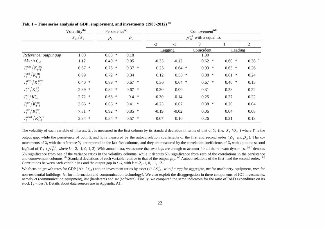
Table 1 reports a number of classical business-cycle time-series indicators (Schlitzer, 1995) to
measure volatility, persistence, and co-movement of each variable of interest (in general, Xt) with respect to
the output gap (i.e. the reference variable).
Table 1 here
The growth rate of GDP and investment in machinery have approximately the same volatility of the
output gap (the reference series) over the cycle, while non-residential investment are significantly less
volatile. ICT investments and its main components, as well as R&D, are twice more volatile than physical
assets. According to the persistence indicators all the variables in Table 1 are broadly stationary, albeit at
different degrees.7 Investment ratios are more persistent than the rate of growth of GDP and employment,
7 The permanent inventory method relating investment and capital stock, t
j
t
j
t
j
t
j
t KKKI 11 //, implies that the
investment ratios in Table 1 are linked to the growth of the capital stocks. Unreported unit root tests show that log-
levels of capital stocks are I(1), as their first differences always reject the null of unit roots.
9
with first order autocorrelations equal to 0.7 or above. Non-residential buildings, software (sw) and R&D
expenditure (berd) show the highest degree of persistency. Finally, GDP growth and investment ratios in
machinery and buildings are pro-cyclical and coincident (or slightly leading), while ICT and R&D
expenditure are a-cyclical (hardware resembles machinery and equipment).
The descriptive analysis supports the idea that Non-ICT physical assets and ICT (but also R&D)
evolve and react differently over the business cycle and that the dynamics of aggregate business investment
is substantially similar to Non-ICT capital.
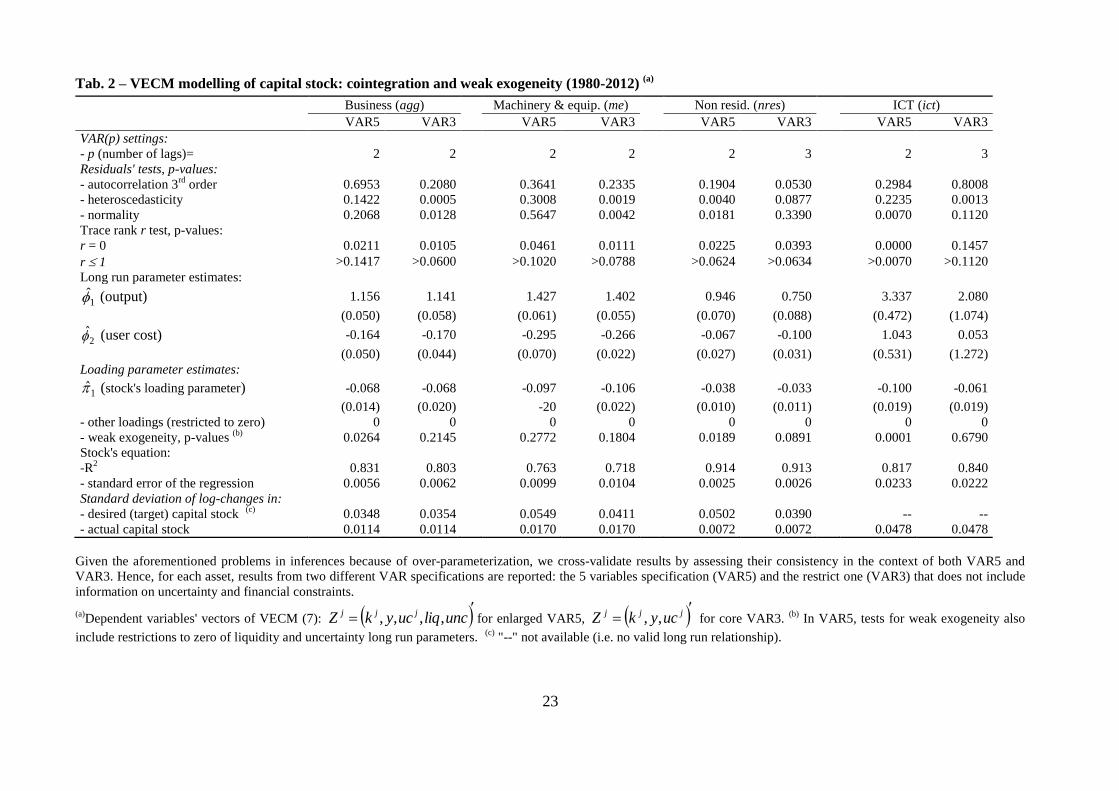
4.2. The cointegration analysis
The cointegration analysis has been performed using the Johansen's rank-test based on VECM (7) at
the aggregate level and by asset. The 5 vector variables includes the three components of the classical capital
stock model together with a measure of uncertainty and a measure of liquidity constraints
uncliqucykZ jjj ,,,, . The estimation results are reported in Table 2.
Table 2 here
A significant cointegration relationship is identified for aggregate stock as well as for Non-ICT
assets while we do not find any cointegration relationship for ICT8 stock. The identified cointegrated vectors
support the relationship between desired capital stock and its classical determinants (output and user costs).
In the long run, aggregate stock and Non-ICT assets adjust to desired stocks whose determinants are weakly
exogenous9.
The long run desired capital stock elasticity to output (restricted VAR3, Table 2) is very close to one
in the aggregate specification, and significantly higher than (lower than) one for machinery and equipment
(for non-residential buildings). The significant negative value (below -1) of the capital stock elasticity to the
user cost rejects the accelerator model but supports the prediction of the flexible neoclassical model.
The speed of adjustment of actual to desired capital stocks is rather slow, suggesting the presence of
dynamics with relevant adjustment costs, especially for non-residential buildings. The long run estimates
above reinforce the prediction of Caballero (1994) that – when there are relevant adjustment costs - the
standard deviations of the desired stocks is larger than the actual stocks10
.
8 The data congruence of VAR models has been assessed through a number of residuals' mis-specification tests, which
hardly ever reject the null of vector white noise errors. In the few cases of failure of the heteroschedasticity and/or the
normality tests, the inclusion of one/two dummies in the deterministic components prevents such rejections without
qualitative changes in the results reported here without such dummies.
9 Columns 1 to 5, show the remarkable similarity of test results and parameter estimates in VAR5 and VAR3 models. In
the trace tests, the cointegration rank is always one at least at 5%, and the weak exogeneity is never 1% significant.
10 The last two rows of Table 2 show that the variability of the business target stock is about three times that of the
actual stock; for machinery and equipment this ratio is slightly lower (suggesting lower adjustment costs than the
10
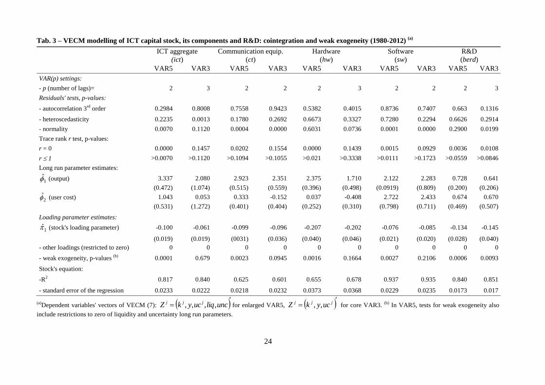
ICT capital stock behaves rather differently. The cointegration rank tests deliver the following
results: the rank is larger than one in VAR5 and zero (no cointegration) in VAR3. As far as VAR5 results are
concerned, the cointegration finding that r>1, together with the strong rejection of the weak exogeneity
restrictions, support the assumption that the underlying long run relationships in reduced form are a
combination of target capital stock determinants and liquidity and uncertainty rather than the classical capital
stock equations. 11
This hypothesis has been tested looking both at the individual ICT components, namely
communication equipment (ct), hardware (hw) and software (sw) and at R&D. The analysis is reported in
Table 3, in which the first two columns for aggregate ICT replicate the last two columns of Table 2 to ease
presentation. Results can be summarized in three main findings.
Table 3 here
First, ICT components and R&D behave as aggregate ICT, hence they react to different determinants
compared to Non-ICT physical capital. Second, the user cost of capital does not play any relevant role in the
long run, as it is never significant and has opposite sign in eight cases out of ten. Third, the weak exogeneity
of uncertainty and liquidity constraints is always strongly rejected.
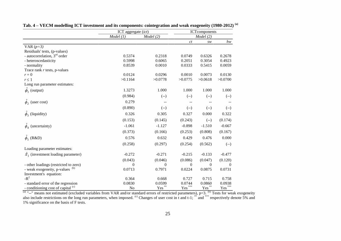
To further improve our understanding of ICT driving factors we test a VECM specification on ICT
investment rather than capital stock. To test for the existence of possible complementarity between ICT and
R&D we extend equation (7) including the log GDP share of R&D (Table 4).
Table 4 here
All variables (including uncertainty) are weakly exogenous: the disequilibria only feed short run
changes in actual investments. The joint restrictions that the elasticity of investment to output is equal to one
and that the elasticity to the user cost is equal to zero (i.e. the user cost plays a transitory role) are not
rejected. Under these restrictions, in the long run, the ICT output ratio (in logs) is positively correlated with
financial liquidity constraints and R&D, and negatively related with uncertainty. In particular, the long run
ICT elasticity to uncertainty is not significantly different from minus one, while the long run effects of
liquidity and R&D are smaller. The speed of adjustment of actual to target ICT investments is estimated
around 0.27 (i.e. about one-quarter of the discrepancy between desired and actual investment is closed after
one year), denoting flow adjustment costs which are considerably lower than the stock adjustment costs
experienced by business, machinery-equipment and non-residential buildings.12
Overall our findings
corroborate the assumption that ICT capital accumulation, as other knowledge based assets (R&D), respond
to macroeconomic shocks differently compared to non-ICT capital (Bloom, 2007).
aggregate), and for non residential buildings this ratio is clearly higher (about five-six times, denoting the highest
adjustment costs).
11 This interpretation is also supported by opposite-signed and/or quite imprecise long run ϕ1 and ϕ2 estimates in the
VAR5 where probably wrong restrictions to identify the long-run capital stock equation are imposed.
12 As for capital stock targets, also ICT investment targets show standard deviations which are larger than the actual
ones (results not reported in Table 4, but available upon request).
11
In table 4 the analysis of ICT investment has been extended to its components: communication
equipment (ct), software (sw) and hardware (hw). The results suggest that each component performs as
aggregate ICT. However, there are some interesting differences in the long run parameters: liquidity does
not exert a long run effect on software, and R&D does not affect hardware. Software reacts strongly to
uncertainty (almost double compare to the other ICT components) while hardware reveals the highest speed
of adjustment. Finally, it is worth noting that the standard error of the aggregate ICT equation is markedly
lower than those of the three disaggregate equations: due to the statistical averaging of the individual shocks,
the aggregate ICT picture is clearer.
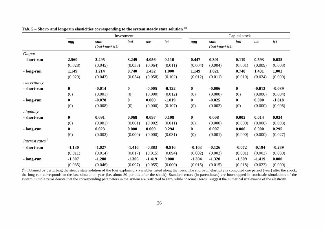
4.3. The elasticities of the investment-capital stock system
We have defined an investment capital stock system of stochastic and deterministic equations where
liquidity constraints and uncertainty interact with the traditional determinants of investment expenditure:
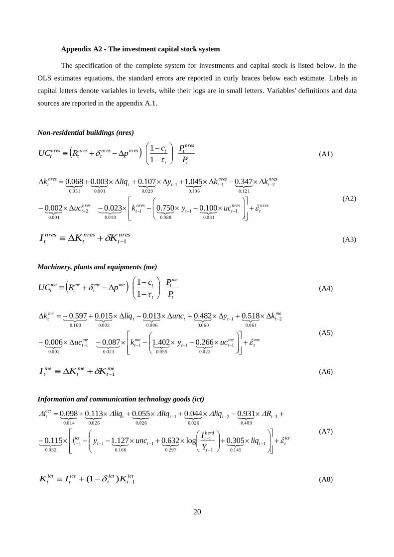
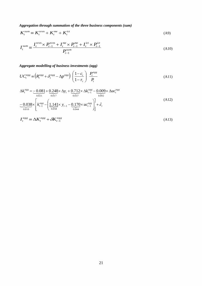
output and user cost (A1-A8 equations in appendix A.2). In the investment capital stock system we evaluate
short and long run composition effects comparing the sensitivity of total (agg) capital stock and investment
(A9-A10) with that of the same variables (sum) obtained summing across the assets (A12-A13).
To characterize the different sensitivity of aggregate and disaggregate investment and capital stock
we derive the steady state solution of the system through its simulation 90 periods ahead where all the un-
modelled variables are assumed to remain constant at the level of the last end-of-sample observation.
Then we calculate the short and long run elasticities13
, of agg and sum variables perturbing our selected
determinants. Table 5 reports the main results.
Table 5 here
The estimated output elasticities tend to significantly differ in the short-run, while the user cost (i.e.
the interest rates) elasticities do not diverge. In the long run, the output elasticity of investment and capital
stock are obviously similar to those estimated by the cointegrated relationships in Table 2 and Table 4. The
zeros corresponding to the agg columns reveal that the aggregate modelling of capital stock admits the
exclusion of uncertainty and liquidity effects, that instead play a significant role in the individual asset
specifications.
The sum outcomes, show that an improvement in the liquidity conditions has an impact about five times
larger than the effect of a reduction of uncertainty. Then the identified long run cointegration between ict
investment and uncertainty, suggests that uncertainty permanently affects ICT expenditure (a 10% increase
in uncertainty reduces the long run business investment level by about 1%), while the liquidity impact
vanishes in the long-run.
13
The standard errors of the elasticity (reported below each elasticity row) are computed on the basis of stochastic
simulations in which the residuals are bootstrapped (1000 replications).
12
5. Policy implications
Our analysis shows that the dynamics of Non-ICT and ICT capital is subject to a different set of
drivers, both in the short- and in the long-run since they respond differently to macroeconomic shocks. From
a policy perspective this is a relevant result suggesting that the identification of asset specific policy design
can be very important to stimulate single and aggregate investment expenditure.
Further, the relatively higher reactivity of ICT supports the idea that in a period of economic
downturn when the opportunity cost of a company’s resources is reduced, so that it has a greater opportunity
to reorganise production and other business processes, there is increasing scope for innovation without
sacrificing growth (Bhaumik, 2011). Therefore during a recession policymakers should definitely stimulate
productivity enhancing investments, such as those in knowledge based assets, to encourage economic
recovery.
We check the sensitivity of technological and non-technological assets to the business cycle
evaluating the effect of uncertainty and firm’s liquidity constraints on the dynamics of Italian Non-ICT and
ICT capital accumulation. The analysis of the channels through which financial constraints and uncertainty14
affected Italian investment dynamics over the recent years is potentially helpful to address the growth
differential between the Italian economy and the average of the other euro area countries.
Since the financial turmoil in 2008, Italy experienced a deep recession. Subsequently, the risk of a
sovereign debt defaults (in the middle of the Greek crisis) and endemic domestic political instability in the
Italian economy fuelled uncertainty. In 2009, as in most of the other developed countries, the Italian GDP
growth slowed down substantially (-5.5%), recovering in 2010 and 2011 (1.8% and 0.7% respectively). In
2012, instead, even though in the euro area the recovery was moderately in progress (German GDP rose by
0.7 while French GDP remained at 0.0), Italy experienced another slowdown (GDP growth decreased by -
2.6%)15
.
The risk of sovereign debt defaults is clearly represented by the Italian index of economic policy
uncertainty showing the markedly higher level of uncertainty experienced since 2008, as compared to the
other European countries (summarised by the average of Germany, France and Spain). The shaded area in
Figure 1 provides a broad idea of the degree of economic and political uncertainty that characterized the
Italian economy over the period..
Figure 1 here
14
In periods of recession high level of uncertainty and low level of liquidity could negatively influence behavioural
responses of firms and consumers as shown in e.g. Romer (1990) and Bloom (2009). The economic rationale of this
effect lies in a number of theoretical underpinnings, based on the channel of real- and growth-options, of the risk premia
and of the precautionary savings (for an updated survey, see Bloom, 2014)
15 The projection for 2013 are still negative (-1.9%), however in Q4 2013, for the first time since Q2 2011 the growth
rate has not been negative.
13
Further, the evolution of the financial conditions, measured by the ISTAT monthly business survey,
reinforces our assumption. In 2012, as reported in Figure 2, in Italy, the level of liquidity was very close to
the low level recorded in 2009.
Figure 2 here
Now our aim is to assess the macroeconomic effects of a change in the level of uncertainty and
liquidity conditions on economic performance, taking into account the intrinsic characteristics of the Italian
economy over the period. To this goal we include the system of equations listed in appendix A2 in the
framework of the Italian Statistical Institute Macroeconometric Model (MeMo-It) 16
to build a counterfactual
exercise - over the period 2008-2013 – to compare the current Italian economic performance with a
simulated scenario where the level of uncertainty is equal to the average of France, Germany and Spain (the
improvement is the shaded area in Figure 1), and the liquidity conditions are constantly improved in 2012-
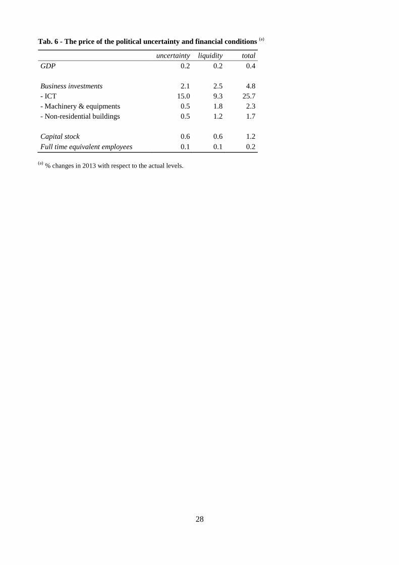
2013 (the measure of the improvement is the shaded area in Figure 2). 17
Table 6 shows that over the years 2008-2013, a lower level of uncertainty and better financial
conditions could account for a cumulate increase of almost 5% in business investments with respect to their
level in 2013, and 1.2% in capital stock. GDP would have been raised by 0.4%, and employment by a
slightly smaller amount (0.2%, corresponding to an increase in the number of full time employees by about
50 thousands).
Table 6 here
Remarkably, Non-ICT and ICT investments react differently to uncertainty and liquidity changes.
Although ICT investment is more sensitive to uncertainty, financial conditions play a relevant role: smaller
uncertainty coupled with higher level of liquidity would make them increase by a cumulate 25% in six years.
Both investments in machinery and equipment and in non-residential buildings react to both shocks, with a
higher sensitivity to the financial conditions (improving by 2.3% and 1.7% respectively).
6. Concluding remarks
In this paper, we modelled the dynamics of business investment taking into account asset specific
characteristics potentially affecting the reactivity of capital accumulation at the aggregate and disaggregate
level over the business cycle. Our analysis corroborates the assumption that ICT and Non-ICT investment
16
MeMo-It is an annual model composed by 53 stochastic equations and 78 identities, and represents a New Keynesian
economic system including households, firms, public administration, and a foreign sector. MeMo-It is structured into
five main blocks supply side, labor market, demand side, prices, and Government. For more details see Bacchini et al.
(2013). Of course, the three disaggregate investment equations replace the pre-existing (aggregated) one.
17 In particular, in the counterfactual the liquidity indicator is assumed to ignore the deep financing trough of 2012, by
shifting back the observations for 2013 and 2014, as if the hole of 2012 never happened. Further,we recognize that our
results are surrounded by the usual caveats emerging from any macro-econometric counterfactual.
14
decisions are driven by a different set of determinants, both in the long- and in the short-run. Additionally,
our finding support the idea that tangible and intangible assets have different speed of adjustments to
macroeconomic shocks because they incur in different adjustment costs. ICT as other knowledge based
assets typically incur in flow adjustment costs thus being more reactive to fluctuations over the business
cycle (Bloom (2007)).
We found that individual investment characteristics matter since we observed highly heterogeneous
behaviour of each asset over the business cycle. In the short run, liquidity constraints and uncertainty are key
determinants of Non-ICT capital accumulation, while ICT investment is driven by the interest rate and
financial constraints. In the long run instead, uncertainty and output have permanent effects on ICT, while
Non-ICT tangible capital is affected by output and the user cost as suggested by the flexible neoclassical
model.
Our simulation results support the idea that ICT is a key variable to assess sound policy measures to
stimulate economic growth. This finding is consistent with the empirical literature that widely demonstrated
that ICT investment generates higher returns to growth than the other capital assets thus producing higher
level of GDP (Jorgenson and Stiroh, 2000, Jorgenson and Vu, 2007).
We tested our model on the Italian data over the period 2008-2013. Simulation results show that better
financial conditions and lower uncertainty could have helped the recovery of the Italian economy after the
Great Recession, mainly through their impact on ICT.
Our findings provide a contribution to the European policy agenda emphasising the central role of
investment specific policy measures necessary to reduce economic growth differentials both inside the union
and with respect to the US. The issue is particularly relevant in the peripheral countries where the increasing
investment gap would probably be substantially reduced stimulating the expenditure in investment
components with higher output elasticities, such as ICT. Future research developments will be devoted to test
our investment capital stock system of equations on a the Eurozone countries with the aim of building a new
framework for investment policy programmes.
15
References
Bacchini , F., C. Brandimarte, P. Crivelli, R. De Santis, M. Fioramanti, A. Girardi, R. Golinelli, C. Jona-
Lasinio, M. Mancini, C. Pappalardo, D. Rossi, M. Ventura and C. Vicarelli (2013), “Building the core
of the Istat system of models for forecasting the Italian economy: MeMo-It”, Rivista di statistica
ufficiale, No. 1, pp. 17-45.
Bachmann, R., R.J. Caballero and E.M.R.A. Engel (2013), "Aggregate implications of lumpy investment:
new evidence and DSGE model", American Economic Journal: Macroeconomics, Vol. 5, No. 4, pp.
29-67.
Baker, S. R., N. Bloom and S. J. Davis (2013), "Measuring Economic Policy Uncertainty", mimeo.
Bhaumik, S. (2011), "Productivity and the economic cycle", BIS Economics Paper, No. 12.
Bernanke B. S. (1983) “Irreversibility, Uncertainty, and Cyclical Investment”, Quarterly Journal of
Economics, Vol. 97, No. 1, pp. 85-106.
Bertola, G. (1988), Adjustment Costs and Dynamic Factor Demands: Investment and Employment Under
Uncertainty, PhD Dissertation, Ch. 2, Massachusetts Institute of Technology.
Bertola G. and R. J. Caballero (1994), “Irreversibility and aggregate investment”, Review of Economic
Studies, Vol. 61, pp. 223-246.
Bianco, M., M. E. Bontempi, R. Golinelli and G. Parigi (2013), "Family firms’ investments, uncertainty and
opacity", Small Business Economics, Vol. 40, No. 4, pp. 1035-1058.
Bloom, N. (2007) “Uncertainty and the Dynamics of R&D,” American Economic Review, 97, 2, 250-255.
Bloom, N. (2009), “The impact of uncertainty shocks”, Econometrica, Vol. 77, No. 3, pp. 623-685.
Bloom, N. (2014), “Fluctuations in uncertainty”, Journal of Economic Perspectives, Vol. 28, No. 2, pp 153-
176.
Bloom, N., S. Bond and J. Van Reenen (2007), "Uncertainty and investment dynamics", Review of Economic
Studies, Vol. 74, No. 2, pp. 391-415.
Bond, S.R. and J.G. Cummins (2000), “The stock market and investment in the new economy: some tangible
facts and intangible fictions”, Brookings Papers on Economic Activity, No. 1, pp. 61-124.
Bond, S.R. and C. Meghir (1994), “Dynamic investment models and the firm’s financial policy”, Review of
Economic Studies, Vol. 61, No. 2, pp. 197-222.
Bontempi, M. E. (2014), “Investment-uncertainty relationship: differences between intangible and physical
capital”, paper invited for presentation at the 4th European Conference on Corporate R&D and
Innovation: Financing R&D and Innovation for Corporate Growth in the EU: Strategies, drivers and
barriers, CONCORDì-2013, European Commission, Seville, 26-27 September 2013.
Bontempi, M. E., A. Del Boca, A. Franzosi, M. Galeotti, and P. Rota (2004), "Capital heterogeneity: does it
matter? Fundamental q and investment on a panel of Italian firms", RAND Journal of Economics, Vol.
35, No. 4, pp. 674-690.
Bontempi, M. E., R. Golinelli and G. Parigi (2010), "Why demand uncertainty curbs investments: evidence
from a panel of Italian firms", Journal of Macroeconomics, Vol. 32, pp. 218-238.
Bontempi, M. E. and J. Mairesse (2014), “Intangible Capital and Productivity at the Firm Level: a Panel
Data Assessment”, Economics of Innovation and New Technology, forthcoming.
Brainard, W. C. and J. Tobin (1968), "Pitfalls in financial model buildings", American Economic Review,
Vol. 58, No. 2, pp. 99-122.
Buti, M. and P. Mohl (2014), “Raising investment in the Eurozone”, http://www.voxeu.org/article/raising-
investment-eurozone
Caballero, R. J. (1994), "Small sample bias and adjustment costs", Review of Economics and Statistics, Vol.
76, No. 1, pp. 52-58.
16
Caballero, R. J. (1999), "Aggregate investment", in J. Taylor and M. Woodford (eds.) Handbook of
Macroeconomics, Vol. 1, Elsevier.
Caballero, R.J., E.M.R.A. Engel and J. C. Haltiwanger (1995), “Plant-Level Adjustment and Aggregate
Investment Dynamics”, Brooking Papers on Economic Activity, No. 2, pp. 1-54.
Carruth, A., A. Dickerson and A. Henley (2000), What Do We Know About Investment Under Uncertainty,
Journal of Economic Surveys, Vol. 14, No. 2, pp. 119-153.
Cequera, D. and G. J. Klein,"Endogenous firm heterogeneity, ICT and R&D incentives", ZEW Discussion
Papers, No. 08-126.
Chirinko, R. (1983), “Investment and Tax policy: a survey of existing models and empirical results with
applications to the high technology sector”, A Report for the National Science Foundation, Division of
Policy Research and Analysis.
Chirinko R. S. (1993), “Business Fixed Investment Spending: A critical Survey of modeling Strategies,
Empirical Results, and Policy Implications”, Journal of Economic Literature, Vol. 31, 4, 1875-1911.
Clark, J. M. (1917), "Business acceleration and the law of demand: a technical factor in economic cycles",
Journal of Political Economy, Vol. 25, pp. 217-235.
Clark, J. M. (1944), "Additional notes on business acceleration and the law of demand", in American
Economic Association, Readings in Business Cycle Theory, Philadelphia, pp. 254-260.
Clark, P. K. (1979), "Investment in the 1970s: Theory, performance, and prediction", Brookings Papers on
Economic Activity, No. 1, pp. 73-113.
Consoli, D. (2012), “Literature analysis on determinant factors and the impact of ICT in SMEs”, Procedia -
Social and Behavioral Sciences, Vol. 62, pp. 93–97.
Cooper, R. W., and J. C. Haltiwanger (2006), “On the Nature of Capital Adjustment Costs”, Review of
Economic Studies, Vol. 73, pp. 611–33.
Czarnitzki, D. and H. Hottenrott (2011), “R&D Investment and Financing Constraints of small and medium-
sized firms”, Small Business Economics, Vol. 36, pp. 65-83.
Czarnitzki, D. and A. A. Toole (2007), “Business R&D and the Interplay of R&D Subsidies and Product
Market Uncertainty”, Review of Industrial Organization, Vol. 31, pp. 169-181.
Czarnitzki, D. and A.A. Toole (2011), “Patent Protection, Market Uncertainty, and R&D Investment”, The
Review of Economics and Statistics, Vol. 93, No. 1, pp. 147-159.
Czarnitzki, D. and A.A. Toole (2013), “The R&D Investment-Uncertainty Relationship: Do Strategic Rivalry
and Firm Size Matter?”, Managerial and Decision Economics, Vol. 34, pp. 15-28.
De Arcangelis, G., C. Jona-Lasinio and S. Manzocchi (2004), "Sectoral determinants and dynamics of ICT
investment in Italy", Rivista di Politica Economica, Vol. 94, No. 3, pp. 119-162.
de Bondt, G., & Diron, M. (2008) “Investment, financing constraints and profit expectations: new macro
evidence”, Applied Economics Letters, Vol. 15, No. 8, pp. 577-581.
Dixit, A.K. and R. S. Pindyck (1994), Investment under Uncertainty, Princeton University Press.
Eisner, R. (1967), "The Permanent Income Theory for Investment: Some empirical explorations", American
Economic Review, Vol. 62, No. 3, pp. 363-390.
Eisner, R. (1969), "Tax policy and investment behavior: a comment", American Economic Review, Vol. 59,
No. 2, pp. 379-388.
Fazzari S.M., R. G. Hubbard, and B. C. Petersen (1988), "Financing constraints and corporate investment",
Brookings Papers on Economic Activity, No. 1, pp. 141.95.
Gaiotti, E. (2013), "Credit availability and investment: Lessons from the Great Recession", European
Economic Review, Vol. 59, pp. 212-227.
17
Goel R. K. and R. Ram (2001), “Irreversibility of R&D investment and the adverse effect of uncertainty:
Evidence from the OECD countries”, Economics Letters, Vol. 71, pp. 287–291.
Gordon, R. J. and J. Veitch (1986), “Fixed Investment in the American Business Cycle, 1919-83” in R. J.
Gordon (ed.), The American Business Cycle: Continuity and Change, NBER, pp. 267-358.
Granger, C. W. J. and N. Haldrup (1997), "Separation in cointegrated systems and persistent-transitory
decompositions", Oxford Bulletin of Economics and Statistics, Vol. 59, No. 4, pp 449-462.
Greasley, D. and J. B. Madsen (2006), “Investment and Uncertainty: Precipitating the Great Depression in
the United States”, Economica, Vol. 73, No. 291, pp. 393–412.
Guerrieri, P, M. Luciani and V. Meliciani (2011), "The determinants of investment in information and
communication technologies", Economics of Innovation and New Technology, Vol. 20, No. 4, pp. 387-
403.
Guiso, L. and G. Parigi (1999), "Investment and demand uncertainty", Quarterly Journal of Economics, Vol.
114, No. 1, pp. 185-227.
Hall, B. H. (2007), “Measuring the returns to R&D: the depreciation problem", NBER Working Paper, No.
13473.
Hall, B. H. and J. Lerner (2010), “The Financing R&D and Innovation”, in B. H. Hall and N. Rosenberg
(eds.) Handbook of the Economics of innovation, Elsevier-North Holland.
Hall, R. E. and D. W. Jorgenson (1967), "Tax policy and investment behavior", American Economic Review,
Vol. 57, No. 3, pp. 391-414.
Hausman, J. A. (1978), "Specification Tests in Econometrics", Econometrica, No. 46, Vol. 6, pp. 1251–
1271.
Himmelberg, C. P. and B. C. Petersen (1994), “R&D and Internal Finance: A panel Study of Small Firms in
High-Tech Industries”, Review of Economics and Statistics, Vol. 76, pp. 38-51.
Hubbard, R.G. (1998), “Capital-market imperfections and investment”, Journal of Economic Literature, Vol.
36, pp. 193-225.
Johansen, S. (1995), Likelihood-based Inference in Cointegrated Vector Autoregressive Models, Oxford
University Press.
Jorgenson, D. W. (1963), "Capital theory and investment behavior", American Economic Review, Vol. 53,
No. 2, pp. 247-259.
Jorgenson, D. W. (2001), "Information Technology and the U.S. Economy", American Economic Review,
Vol. 91, No. 1, pp. 1–32.
Jorgenson, D. W. and K. J. Stiroh (1999), "Information Technology and Growth", American Economic
Review, Vol. 89, No. 2, pp. 109–115.
Jorgenson, D. W. and K. Vu (2007), "Information technology and the world growth resurgence", German
Economic Review, Vol. 8, No. 2, pp. 125–145.
Kang, W., K. Lee and R. A. Ratti (2014), "Economic Policy uncertainty and firm-level investment", Journal
of Macroeconomics, Vol. 39, pp. 42-53.
Koyck, L. M. (1954), Distributed Lags and Investment Analysis, North Holland, Amsterdam.
Leahy, J. V. and T. M. Whited (1996), "The Effect of Uncertainty on Investment: Some Stylized Facts",
Journal of Money Credit and Banking, Vol. 28, pp. 64-83.
Lee, J. and P. Rabanal (2010), "Forecasting US investment", IMF Working Paper, No. 246.
McDonald, R. and D. Siegel (1986), “The Value of Waiting to Invest”, Quarterly Journal of Economics,
Vol. 101, No. 4, 707-728.
O'Mahony, M. and M. Vecchi (2005), "Quantifying the impact of ICT capital on output growth: a
heterogeneous dynamic panel approach", Economica, Vol. 72, No. 288, pp. 615-633.
18
Parigi, G. and S. Siviero (2001), "An investment-function-based measure of capacity utilisation. Potential
output and utilised capacity in the Bank of Italy's quarterly model", Economic Modelling, Vol. 18, pp.
525-550.
Pesaran, M.H., Y. Shin and R. J. Smith (2001), "Bounds approaches to the analysis of level relationships",
Journal of Applied Econometrics, Vol. 16, pp. 289–326.
Pindyck, R. S (1988), “Irreversible Investment, Capacity Choice, and the Value of the Firm”, American
Economic Review, Vol. 78, No. 5, pp. 969-985.
Pindyck, R. S (1991), “Irreversibility, Uncertainty, and Investment”, Journal of Economic Literature, Vol.
29, n. 3, pp. 1110-48.
Qin, D. (2011), "Rise of VAR modelling approach", Journal of Economic Surveys, Vol. 25, pp. 156-174.
Romer, C. (1990), “The Great Crash and the Onset of the Great Depression”, Quarterly Journal of
Economics, Vol. 105, No. 3, pp. 597– 624.
Schlitzer, G. (1995), “Business cycles in Italy: A statistical investigation”, European Journal of Political
Economy, Vol. 11, pp. 683-698.
Stein, L. C. and E. C. Stone (2012), "The effect of uncertainty on investment, hiring, and R&D: Causal
evidence from equity options, mimeo.
Stock, J. H. and M. W. Watson (1993), "A simple MLE of cointegrating vectors in higher order integrated
systems", Econometrica, Vol. 61, No. 4, pp. 783-820.
Tobin, J. (1969), "A general equilibrium approach to monetary theory", Journal of Money, Credit and
Banking, Vol. 1, pp. 15-29.
Tobin, J. and W. C. Brainard (1977), "Asset markets and the cost of capital", in R. Nelson and B. Balassa
(eds.), Economic Progress: Private Values and Public Policy. Essays in Honor of W. Fellner, North
Holland, pp. 235–62.
Urbain, J.-P. (1992), "On weak exogeneity in error correction models", Oxford Bulletin of Economics and
Statistics, Vol. 54, No. 2, pp. 187-207.
Van Leeuwen, G., P. Mohnen, M. Polder and W. Raymond (2009), "Productivity effects of innovation
modes", Statistics Netherlands, paper for ASIGO conference, Nurnberg, May.
Van Reenen, J., N. Bloom, M. Draca, T. Kretschmer, R. Sadun, H. Overman and M. Schankerman (2010).
“The economic impact of ICT”, Final Report, Centre for Economic Performance, SMART No.
2007/0020.
Venturini, F. (2009), "The long-run impact of ICT", Empirical Economics, Vol. 37, No. 3, pp. 497-515.
Whited T.M. (1994), “Problems with Identifying Adjustment Costs from Regressions of Investment on q”,
Economics Letters, Vol. 46, 339-344.
19
Appendix A1 - Data sources
Aggregate (j = agg) and disaggregate (j = me, nres, ict) capital stock and investments data are drawn from
the ISTAT National Accounts (NA) and they refer to the Italian business over the period 1980-2012.
Series are available at both current prices and in volumes (chained index). Non-residential capital stock
(nres) is the difference between business capital stock (agg), machinery and equipment (me) and ICT (ict).
From the NA source, we can compute the series of capital stock and investments in volume, respectively j
tK
and j
tI , and the corresponding series of investment deflators j
tP , obtained as ratios between investments at
current prices and those in volumes.
Output series is measured by GDP in volumes. In the user cost’s formula (3): tP is the GDP deflator; j
t is
the rate of change of investment prices (measured by j
tPlog ); the rate of investments' subsidies (tc ) is the
ratio between Government subsidies to investments and the value of business investments in the previous
year. The cost of borrowing j
tR is given by the average of the rate of interest of long terms Government
bonds (BTP) and ISTAT estimates of the rate of interest implicitly used in collecting information to compute
capital stocks; the arbitrary risk premium (j ) is set to zero. Finally, depreciation rates are obtained by
reversing the formula of the perpetual inventory method, as j
t
j
t
j
tj
tK
KI
1
; the corporate tax rate ( t ) is
obtained by the series of effective tax rates from the NA source.
The degree of financial constraints (liq) is from the ISTAT monthly business survey where it is asked to the
firms: "how do you judge the current level of liquidity (quite good, normal, bad)?". The index of economic
policy uncertainty (unc) is from Backer et al. (2013) and is downloadable from
http://www.policyuncertainty.com.
Nominal R&D is measured by the total intramural R&D expenditure of the Italian business enterprise sector
(source: Eurostat's Statistics on Research and Development). R&D in real terms (berd
tI ) is obtained by
deflating its values with the GDP deflator. In order to compute the R&D stock, we used the perpetual
inventory method with constant depreciation rate (assumed, as customary, equal to about 0.4 - see e.g. Hall,
2007, and Bontempi and Mairesse, 2014). In steady state, the initial value of the capital stock is proxied by
4.0/berd
o
berd
o IK . Although we acknowledge that this is a very crude method, it is just an early estimate
subject to possible improvements.
The output gap series is from the Ameco database of the European Commission.
20
Appendix A2 - The investment capital stock system
The specification of the complete system for investments and capital stock is listed below. In the
OLS estimates equations, the standard errors are reported in curly braces below each estimate. Labels in
capital letters denote variables in levels, while their logs are in small letters. Variables' definitions and data
sources are reported in the appendix A.1.
Non-residential buildings (nres)
t
nres
t
t
tnresnres
t
nres
t
nres
tP
PcpRUC
1
1 (A1)
nres
t
nres
tt
nres
t
nres
t
nres
t
nres
ttt
nres
t
ucykuc
kkyliqk
100.0750.0023.0002.0
347.0045.1107.0003.0068.0
1
031.0
1
088.0
1
010.0
2
001.0
2
121.0
1
136.0
1
029.0001.0031.0
(A2)
nres
t
nres
t
nres
t KKI 1 (A3)
Machinery, plants and equipments (me)
t
me
t
t
tmeme
t
me
t
me
tP
PcpRUC
1
1 (A4)
me
t
me
tt
me
t
me
t
me
tttt
me
t
ucykuc
kyuncliqk
266.0402.1087.0006.0
518.0482.0013.0015.0597.0
1
022.0
1
055.0
1
023.0
1
002.0
2
061.0
1
060.0006.0002.0160.0
(A5)
me
t
me
t
me
t KKI 1 (A6)
Information and communication technology goods (ict)
ict
tt
t
berd
ttt
ict
t
tttt
ict
t
liqY
Iuncyi
Rliqliqliqi
ˆ305.0log632.0127.1115.0
931.0044.0055.0113.0098.0
1
145.01
1
297.0
1
166.0
11
032.0
1
489.0
2
026.0
1
026.0026.0014.0
(A7)
ict
t
ict
t
ict
t
ict
t KIK 1)1( (A8)
21
Aggregation through summation of the three business components (sum)
ict
t
me
t
nres
t
sum
t KKKK (A9)
sum
t
ict
t
ict
t
me
t
me
t
nres
t
nres
tsum
tP
PIPIPII
1
111
(A10)
Aggregate modelling of business investments (agg)
t
agg
t
t
taggagg
t
agg
t
agg
tP
PcpRUC
1
1 (A11)
t
agg
tt
agg
t
agg
t
agg
tt
agg
t
ucyk
uckyk
170.0141.1038.0
009.0712.0248.0081.0
1
044.0
1
058.0
1
010.0
002.0
1
037.0017.0021.0
(A12)
agg
t
agg
t
agg
t KKI 1 (A13)
22
Tab. 1 – Time series analysis of GDP, employment, and investments (1980-2012) (a)
Volatility
(b)
Persistence
(c)
Comovement
(d)
YX 1
2
)(k
XY with k equal to:
-2 -1
0
1
2
Lagging Coincident Leading
Reference: output gap 1.00
0.63 * 0.18
1.00
1 tt YY 1.12
0.40 * 0.05
-0.33 -0.12
0.62 * 0.60 * 0.38 *
aggt
aggt KI 1
0.57 *
0.75 * 0.37 *
0.25 0.64 * 0.93 * 0.63 * 0.26
met
met KI 1 0.99
0.72 * 0.34
0.12 0.58 * 0.88 * 0.61 * 0.24
nrest
nrest KI 1 0.40 *
0.89 * 0.67 *
0.36 0.64 * 0.67 * 0.40 * 0.15
ictt
ictt KI 1 2.89 *
0.82 * 0.67 *
-0.30 0.00
0.31
0.28
0.22
ctt
ctt KI 1 2.72 *
0.68 * 0.4 *
-0.30 -0.14
0.25
0.27
0.22
hwt
hwt KI 1 3.66 *
0.66 * 0.41 *
-0.23 0.07
0.38 * 0.20
0.04
swt
swt KI 1 7.31 *
0.92 * 0.85 *
-0.19 -0.02
0.06
0.04
0.08
berdt
berdt KI 1 2.34 * 0.84 * 0.57 * -0.07 0.10
0.26 0.21 0.13
The volatility of each variable of interest, Xt , is measured in the first column by its standard deviation in terms of that of Yt (i.e. YX / ) where Yt is the
output gap, while the persistence of both Xt and Yt is measured by the autocorrelation coefficients of the first and second order ( 1 and 2 ). The co-
movements of Xt with the reference Yt are reported in the last five columns, and they are measured by the correlation coefficients of Xt with up to the second
lag/lead of Yt-k ()(k
XY , where k= -2, -1, 0, 1, 2). With annual data, we assume that two lags are enough to account for all the relevant dynamics. (a)
* denotes
5% significance from one of the variance ratios in the volatility columns, while it denotes 5% significance from zero of the correlations in the persistence
and comovement columns. (b)
Standard deviations of each variable relative to that of the output gap. (c)
Autocorrelations of the first- and the second-order. (d)
Correlations between each variable in t and the output gap in t+k, with k = -2, -1, 0, +1, +2.
We focus on growth rates for GDP ( 1/ tt YY ) and on investment ratios by asset (j
t
j
t KI 1/ , with j = agg for aggregate, me for machinery-equipment, nres for
non-residential buildings, ict for information and communication technology). We also exploit the disaggregation in three components of ICT investments,
namely ct (communication equipment), hw (hardware) and sw (software). Finally, we computed the same indicators for the ratio of R&D expenditure on its
stock ( j = berd). Details about data sources are in Appendix A1.
23
Tab. 2 – VECM modelling of capital stock: cointegration and weak exogeneity (1980-2012) (a)
Business (agg) Machinery & equip. (me) Non resid. (nres) ICT (ict)
VAR5 VAR3 VAR5 VAR3 VAR5 VAR3 VAR5 VAR3
VAR(p) settings:
- p (number of lags)= 2 2
2 2
2 3
2 3
Residuals' tests, p-values:
- autocorrelation 3rd
order 0.6953 0.2080
0.3641 0.2335
0.1904 0.0530
0.2984 0.8008
- heteroscedasticity 0.1422 0.0005
0.3008 0.0019
0.0040 0.0877
0.2235 0.0013
- normality 0.2068 0.0128
0.5647 0.0042
0.0181 0.3390
0.0070 0.1120
Trace rank r test, p-values:
r = 0 0.0211 0.0105
0.0461 0.0111
0.0225 0.0393
0.0000 0.1457
r 1 >0.1417 >0.0600
>0.1020 >0.0788
>0.0624 >0.0634
>0.0070 >0.1120
Long run parameter estimates:
1 (output) 1.156 1.141
1.427 1.402
0.946 0.750
3.337 2.080
(0.050) (0.058)
(0.061) (0.055)
(0.070) (0.088)
(0.472) (1.074)
2 (user cost) -0.164 -0.170
-0.295 -0.266
-0.067 -0.100
1.043 0.053
(0.050) (0.044)
(0.070) (0.022)
(0.027) (0.031)
(0.531) (1.272)
Loading parameter estimates:
1 (stock's loading parameter) -0.068 -0.068
-0.097 -0.106
-0.038 -0.033
-0.100 -0.061
(0.014) (0.020)
-20 (0.022)
(0.010) (0.011)
(0.019) (0.019)
- other loadings (restricted to zero) 0 0
0 0
0 0
0 0
- weak exogeneity, p-values (b)
0.0264 0.2145
0.2772 0.1804
0.0189 0.0891
0.0001 0.6790
Stock's equation:
-R2 0.831 0.803
0.763 0.718
0.914 0.913
0.817 0.840
- standard error of the regression 0.0056 0.0062
0.0099 0.0104
0.0025 0.0026
0.0233 0.0222
Standard deviation of log-changes in:
- desired (target) capital stock (c)
0.0348 0.0354
0.0549 0.0411
0.0502 0.0390
-- --
- actual capital stock 0.0114 0.0114 0.0170 0.0170 0.0072 0.0072 0.0478 0.0478
Given the aforementioned problems in inferences because of over-parameterization, we cross-validate results by assessing their consistency in the context of both VAR5 and
VAR3. Hence, for each asset, results from two different VAR specifications are reported: the 5 variables specification (VAR5) and the restrict one (VAR3) that does not include
information on uncertainty and financial constraints.
(a)Dependent variables' vectors of VECM (7): uncliqucykZ jjj ,,,, for enlarged VAR5, jjj ucykZ ,, for core VAR3.
(b) In VAR5, tests for weak exogeneity also
include restrictions to zero of liquidity and uncertainty long run parameters. (c)
"--" not available (i.e. no valid long run relationship).
24
Tab. 3 – VECM modelling of ICT capital stock, its components and R&D: cointegration and weak exogeneity (1980-2012) (a)
ICT aggregate
(ict)
Communication equip.
(ct)
Hardware
(hw)
Software
(sw)
R&D
(berd)
VAR5 VAR3 VAR5 VAR3 VAR5 VAR3 VAR5 VAR3 VAR5 VAR3
VAR(p) settings:
- p (number of lags)= 2 3 2 2 2 3 2 2 2 3
Residuals' tests, p-values:
- autocorrelation 3rd
order 0.2984 0.8008 0.7558 0.9423 0.5382 0.4015 0.8736 0.7407 0.663 0.1316
- heteroscedasticity 0.2235 0.0013 0.1780 0.2692 0.6673 0.3327 0.7280 0.2294 0.6626 0.2914
- normality 0.0070 0.1120 0.0004 0.0000 0.6031 0.0736 0.0001 0.0000 0.2900 0.0199
Trace rank r test, p-values:
r = 0 0.0000 0.1457 0.0202 0.1554 0.0000 0.1439 0.0015 0.0929 0.0036 0.0108
r 1 >0.0070 >0.1120 >0.1094 >0.1055 >0.021 >0.3338 >0.0111 >0.1723 >0.0559 >0.0846
Long run parameter estimates:
1 (output) 3.337 2.080 2.923 2.351 2.375 1.710 2.122 2.283 0.728 0.641
(0.472) (1.074) (0.515) (0.559) (0.396) (0.498) (0.0919) (0.809) (0.200) (0.206)
2 (user cost) 1.043 0.053 0.333 -0.152 0.037 -0.408 2.722 2.433 0.674 0.670
(0.531) (1.272) (0.401) (0.404) (0.252) (0.310) (0.798) (0.711) (0.469) (0.507)
Loading parameter estimates:
1 (stock's loading parameter) -0.100 -0.061 -0.099 -0.096 -0.207 -0.202 -0.076 -0.085 -0.134 -0.145
(0.019) (0.019) (0031) (0.036) (0.040) (0.046) (0.021) (0.020) (0.028) (0.040)
- other loadings (restricted to zero) 0 0 0 0 0 0 0 0 0 0
- weak exogeneity, p-values (b)
0.0001 0.679 0.0023 0.0945 0.0016 0.1664 0.0027 0.2106 0.0006 0.0093
Stock's equation:
-R2 0.817 0.840 0.625 0.601 0.655 0.678 0.937 0.935 0.840 0.851
- standard error of the regression 0.0233 0.0222 0.0218 0.0232 0.0373 0.0368 0.0229 0.0235 0.0173 0.017
(a)Dependent variables' vectors of VECM (7): uncliqucykZ jjj ,,,, for enlarged VAR5, jjj ucykZ ,, for core VAR3.
(b) In VAR5, tests for weak exogeneity also
include restrictions to zero of liquidity and uncertainty long run parameters.
25
Tab. 4 – VECM modelling ICT investment and its components: cointegration and weak exogeneity (1980-2012) (a)
ICT aggregate (ict)
ICTcomponents
Model (1) Model (2)
Model (2)
ct sw hw
VAR (p=3)
Residuals' tests, (p-values)
- autocorrelation, 3rd
order 0.5374 0.2318
0.0749 0.6326 0.2678
- heteroscedasticity 0.5998 0.6065
0.2051 0.3054 0.4923
- normality 0.8539 0.0010
0.0333 0.5415 0.0059
Trace rank r tests, p-values
r = 0 0.0124 0.0296
0.0010 0.0073 0.0130
r 1 >0.1164 >0.0778
>0.0775 >0.0618 >0.0700
Long run parameter estimates:
1 (output) 1.3273 1.000
1.000 1.000 1.000
(0.984) (--)
(--) (--) (--)
2 (user cost) 0.279 --
-- -- --
(0.890) (--)
(--) (--) (--)
3 (liquidity) 0.326 0.305
0.327 0.000 0.322
(0.153) (0.145)
(0.243) (--) (0.174)
4 (uncertainty) -1.061 -1.127
-0.898 -1.510 -0.667
(0.373) (0.166)
(0.253) (0.808) (0.167)
5 (R&D) 0.576 0.632
0.429 0.476 0.000
(0.258) (0.297)
(0.254) (0.562) (--)
Loading parameter estimates:
1 (investment loading parameter) -0.272 -0.271
-0.215 -0.133 -0.477
(0.043) (0.046)
(0.086) (0.047) (0.120)
- other loadings (restricted to zero) 0 0
0 0 0
- weak exogeneity, p-values (b)
0.0713 0.7971
0.0224 0.0875 0.0731
Investment's equation:
-R2 0.364 0.668
0.727 0.715 0.758
- standard error of the regression 0.0830 0.0599
0.0744 0.0860 0.0938
- conditioning cost of capital (c)
No Yes **
Yes ***
Yes **
Yes ***
(a) "--" means not estimated (excluded variables from VAR and/or standard errors of restricted parameters), p=3.
(b) Tests for weak exogeneity
also include restrictions on the long run parameters, when imposed. (c)
Changes of user cost in t and t-1; **
and ***
respectively denote 5% and
1% significance on the basis of F tests.
26
Tab. 5 – Short- and long-run elasticities corresponding to the system steady state solution (a)
Investment Capital stock
agg sum (bui+me+ict)
bui me ict agg sum (bui+me+ict)
bui me ict
Output
- short-run 2.560 3.495 3.249 4.056 0.110
0.447 0.301 0.119 0.593 0.035
(0.028) (0.045) (0.038) (0.064) (0.011)
(0.004) (0.004) (0.001) (0.009) (0.003)
- long-run 1.149 1.214 0.740 1.432 1.000
1.149 1.021 0.740 1.431 1.002
(0.029) (0.043) (0.054) (0.058) (0.102)
(0.012) (0.011) (0.010) (0.024) (0.090)
Uncertainty
- short-run 0 -0.014 0 -0.005 -0.122
0 -0.006 0 -0.012 -0.039
(0) (0.001) (0) (0.000) (0.012)
(0) (0.000) (0) (0.000) (0.004)
- long-run 0 -0.078 0 0.000 -1.019
0 -0.025 0 0.000 -1,018
(0) (0.008) (0) (0.000) (0.107)
(0) (0.002) (0) (0.000) (0.096)
Liquidity
- short-run 0 0.091 0.068 0.097 0.108
0 0.008 0.002 0.014 0.034
(0) (0.001) (0.001) (0.002) (0.011)
(0) (0.000) (0.000) (0.000) (0.003)
- long-run 0 0.023 0.000 0.000 0.294
0 0.007 0.000 0.000 0.295
(0) (0.002) (0.000) (0.000) (0.031)
(0) (0.001) (0.000) (0.000) (0.027)
Interest rates b
- short-run -1.130 -1.027 -1.416 -0.883 -0.916
-0.163 -0.126 -0.072 -0.194 -0.289
(0.011) (0.014) (0.017) (0.015) (0.094)
(0.002) (0.002) (0.001) (0.003) (0.030)
- long-run -1.307 -1.280 -1.306 -1.419 0.000
-1.304 -1.320 -1,309 -1.419 0.000
(0.035) (0.046) (0.097) (0.055) (0.000)
(0.015) (0.015) (0.018) (0.023) (0.000)
(a) Obtained by perturbing the steady state solution of the four explanatory variables listed along the rows. The short-run elasticity is computed one period (year) after the shock,
the long run corresponds to the last simulation year (i.e. about 80 periods after the shock). Standard errors (in parentheses) are boostrapped in stochastic simulations of the
system. Simple zeros denote that the corresponding parameters in the system are restricted to zero, while "decimal zeros" suggest the numerical irrelevance of the elasticity.

27
28
Tab. 6 - The price of the political uncertainty and financial conditions (a)
uncertainty liquidity total
GDP 0.2 0.2 0.4
Business investments 2.1 2.5 4.8
- ICT 15.0 9.3 25.7
- Machinery & equipments 0.5 1.8 2.3
- Non-residential buildings 0.5 1.2 1.7
Capital stock 0.6 0.6 1.2
Full time equivalent employees 0.1 0.1 0.2
(a)
% changes in 2013 with respect to the actual levels.
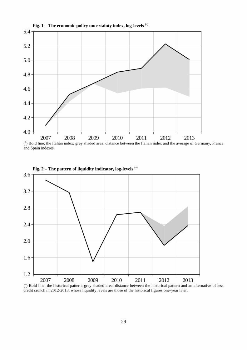
29
Fig. 1 – The economic policy uncertainty index, log-levels (a)
4.0
4.2
4.4
4.6
4.8
5.0
5.2
5.4
2007 2008 2009 2010 2011 2012 2013 (
a) Bold line: the Italian index; grey shaded area: distance between the Italian index and the average of Germany, France
and Spain indexes.
Fig. 2 – The pattern of liquidity indicator, log-levels (a)
1.2
1.6
2.0
2.4
2.8
3.2
3.6
2007 2008 2009 2010 2011 2012 2013 (
a) Bold line: the historical pattern; grey shaded area: distance between the historical pattern and an alternative of less
credit crunch in 2012-2013, whose liquidity levels are those of the historical figures one-year later.


