ICPSR General Structural Equation Models

Week 4 # 3

Panel Data

(including Growth Curve Models)

Causal models:

Ksi-1

Ksi-2 Eta-2

ga2,1

Eta-1

ga1,2

1

1

Cross-lagged panel coefficients

[Reduced form of model on next slide]

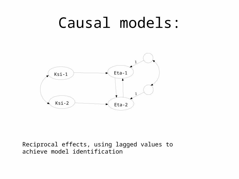
Causal models:

Reciprocal effects, using lagged values to achieve model identification

Ksi-1

Ksi-2 Eta-2

Eta-1

1

1

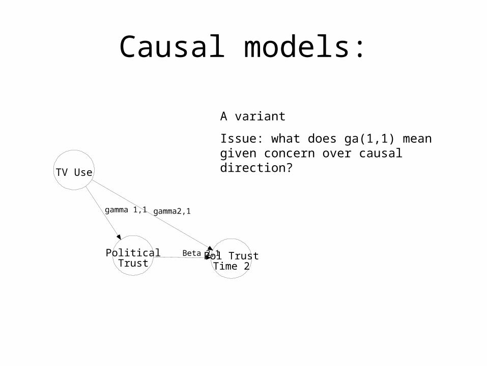
Causal models:

TV Use

PoliticalTrust

Pol TrustTime 2

gamma 1,1 gamma2,1

Beta 2,1

A variant

Issue: what does ga(1,1) mean given concern over causal direction?

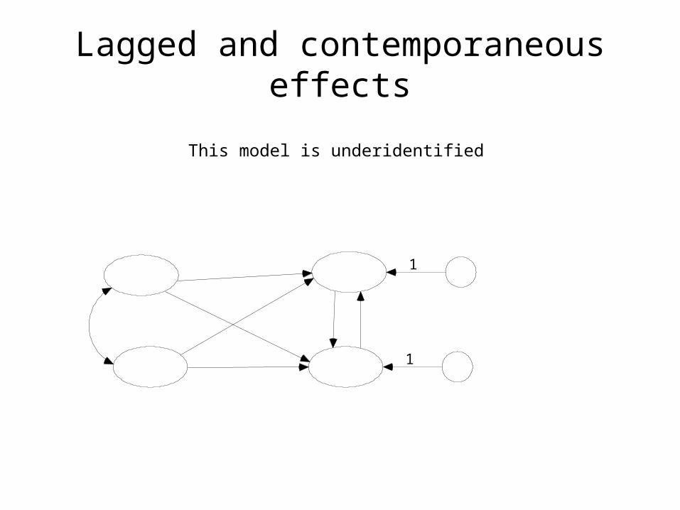
Lagged and contemporaneous effects

1

1

This model is underidentified

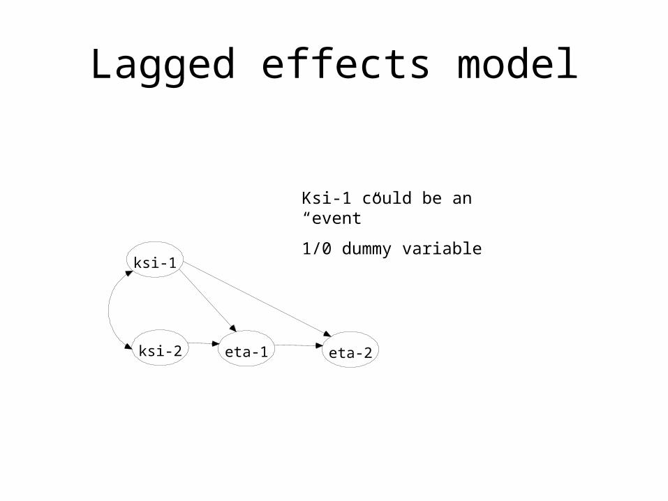
Lagged effects model

ksi-2 eta-1 eta-2

ksi-1

Ksi-1 could be an “event”

1/0 dummy variable

First order model for three wave data(univariate)

1

1 1 1

1

1 1 1

1

1 1 1

Time 1 Time 2 Time 3

First order model for three wave data(univariate)

1

1 1 1

1

1 1 1

1

1 1 1

b1 b1

Tests: Equivalent of stability coefficients (b1)

Mean differences (see earlier slide)

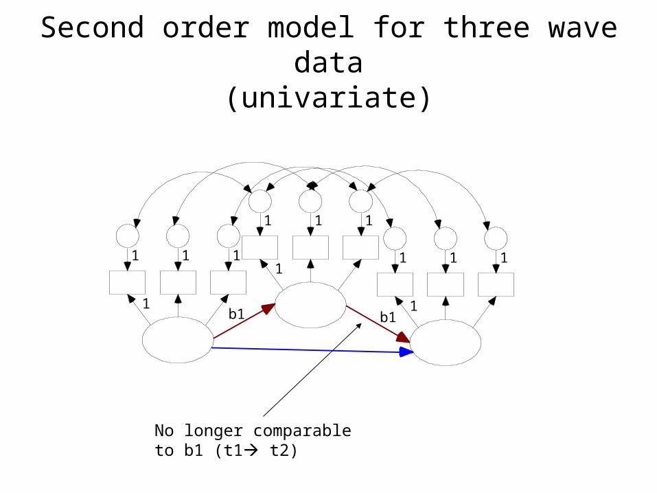
Second order model for three wave data(univariate)

1

1 1 11

1 1 1

1

1 1 1

b1 b1

No longer comparable to b1 (t1 t2)

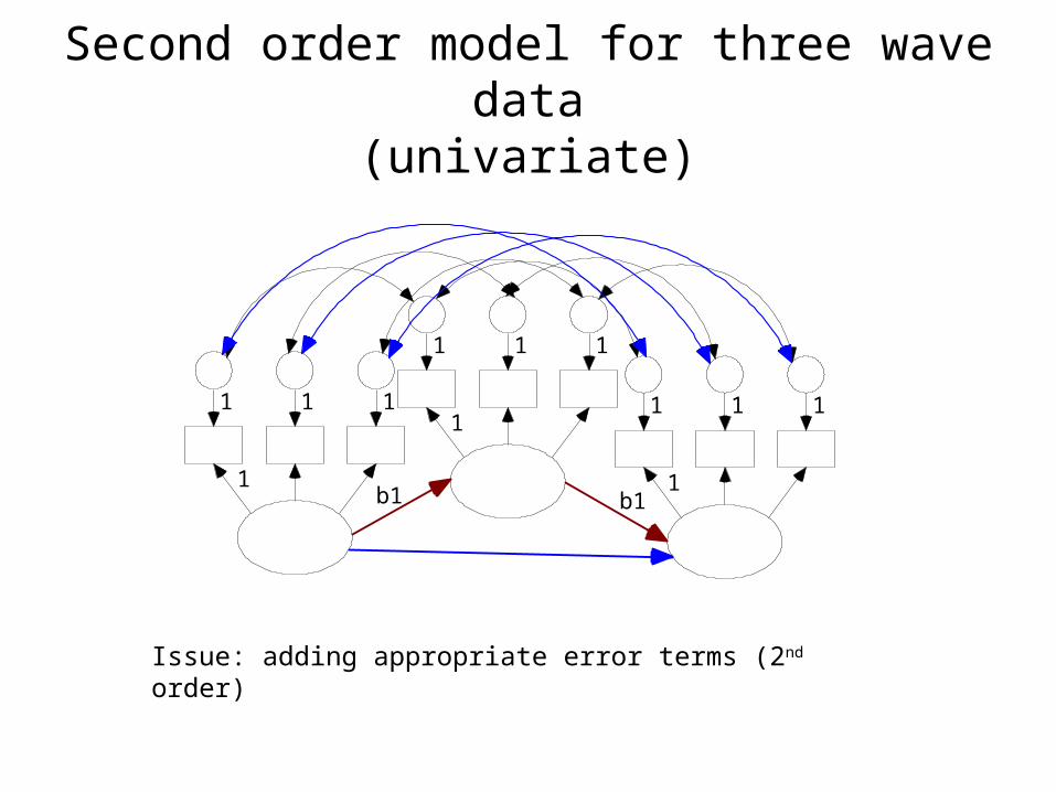
Second order model for three wave data(univariate)

1

1 1 11

1 1 1

1

1 1 1

b1 b1

Issue: adding appropriate error terms (2nd order)

Multivariate Model for Three-wave panel data: cross-lagged effects (first order)

1

1

1

1

Multivariate Model for Three-wave panel data: cross-lagged effects (first order)

1

1

1

1

Equivalence of parameters:

T1 T2

T2 T3

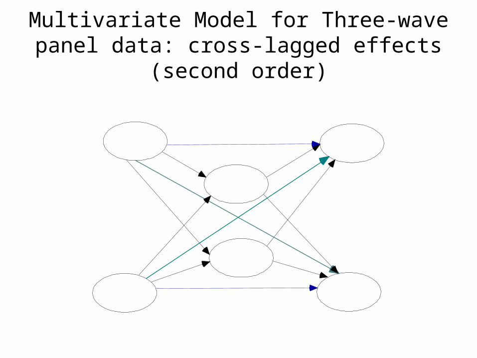
Multivariate Model for Three-wave panel data: cross-lagged effects (second order)

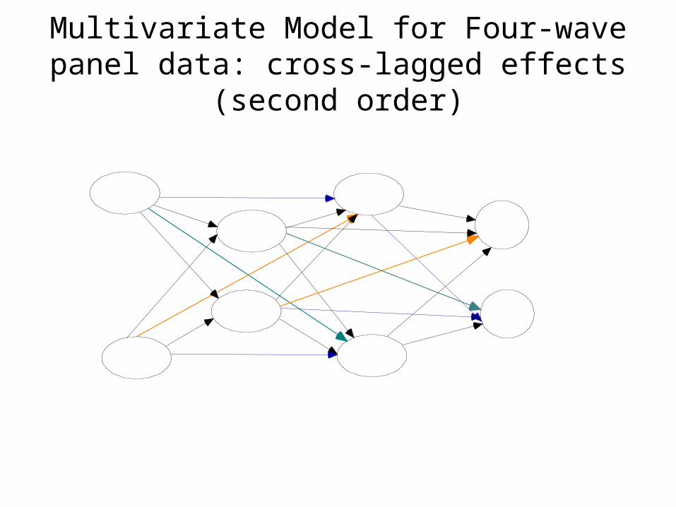
Multivariate Model for Four-wave panel data: cross-lagged effects (second order)

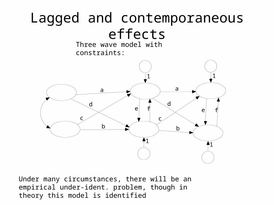
Lagged and contemporaneous effectsThree wave model with constraints:

a

e f

b

d

c

1

1

a

b

e f

1

1

d

c

Under many circumstances, there will be an empirical under-ident. problem, though in theory this model is identified

Example:

• Canada, Quality of Life data

• In directory \Panel in

Week4Examples

Panel Data model

Model for attitudes about labour unions, 1977-1979

Items: 5-pt. agree/disagree199D QD6B Unions too much power Q156C QK16F Scabs (gov’t prohibit

strikebreakers)Q156D QK16G Workers on BoardsQ156B QK16E Teachers should not have

right to strike

Source: Cdn. Quality of life panel study, 1977-1979 waves

Union Atts1977

1

1111

Union atts1979

1

1111

1

Panel Data model

LISREL Estimates (Maximum Likelihood)

LAMBDA-Y

LABOR77 LABOR79 -------- -------- Q199D 1.000 - - Q156C -1.803 - - (0.141) -12.796 Q156D -1.148 - - (0.101) -11.350 Q156B 0.789 - - (0.098) 8.040 QD7B - - 1.000 QK16F - - -1.352 (0.109) -12.355 QK16G - - -0.755 (0.072) -10.479 QK16E - - 0.709 (0.084) 8.427

Panel Data model

BETA

LABOR77 LABOR79 -------- -------- LABOR77 - - - - LABOR79 1.420 - - (0.138) 10.318

PSI Note: This matrix is diagonal.

LABOR77 LABOR79 -------- -------- 0.125 -0.066 (0.017) (0.018) 7.529 -3.611

Squared Multiple Correlations for Structural Equations

LABOR77 LABOR79 -------- -------- - - 1.356

W_A_R_N_I_N_G: PSI is not positive definite

Panel Data model

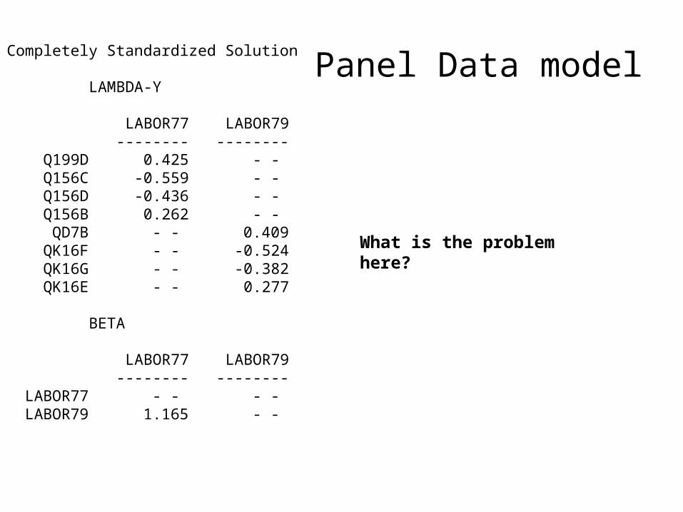
Completely Standardized Solution

LAMBDA-Y

LABOR77 LABOR79 -------- -------- Q199D 0.425 - - Q156C -0.559 - - Q156D -0.436 - - Q156B 0.262 - - QD7B - - 0.409 QK16F - - -0.524 QK16G - - -0.382 QK16E - - 0.277

BETA

LABOR77 LABOR79 -------- -------- LABOR77 - - - - LABOR79 1.165 - -

What is the problem here?

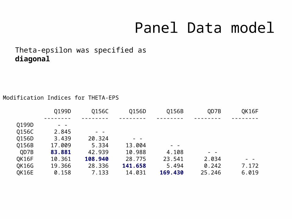
Panel Data model

Theta-epsilon was specified as diagonal

Modification Indices for THETA-EPS

Q199D Q156C Q156D Q156B QD7B QK16F -------- -------- -------- -------- -------- -------- Q199D - - Q156C 2.845 - - Q156D 3.439 20.324 - - Q156B 17.009 5.334 13.004 - - QD7B 83.881 42.939 10.988 4.108 - - QK16F 10.361 108.940 28.775 23.541 2.034 - - QK16G 19.366 28.336 141.658 5.494 0.242 7.172 QK16E 0.158 7.133 14.031 169.430 25.246 6.019

Panel Data model

Union Atts1977

1

1111

Union atts1979

1

1111

1

Panel Data model

Added error covariances:

FR TE 5 1 TE 6 2 TE 7 3 TE 8 4

BETA

LABOR77 LABOR79 -------- -------- LABOR77 - - - - LABOR79 1.094 - - (0.115) 9.547

Covariance Matrix of ETA

LABOR77 LABOR79 -------- -------- LABOR77 0.116 LABOR79 0.127 0.199

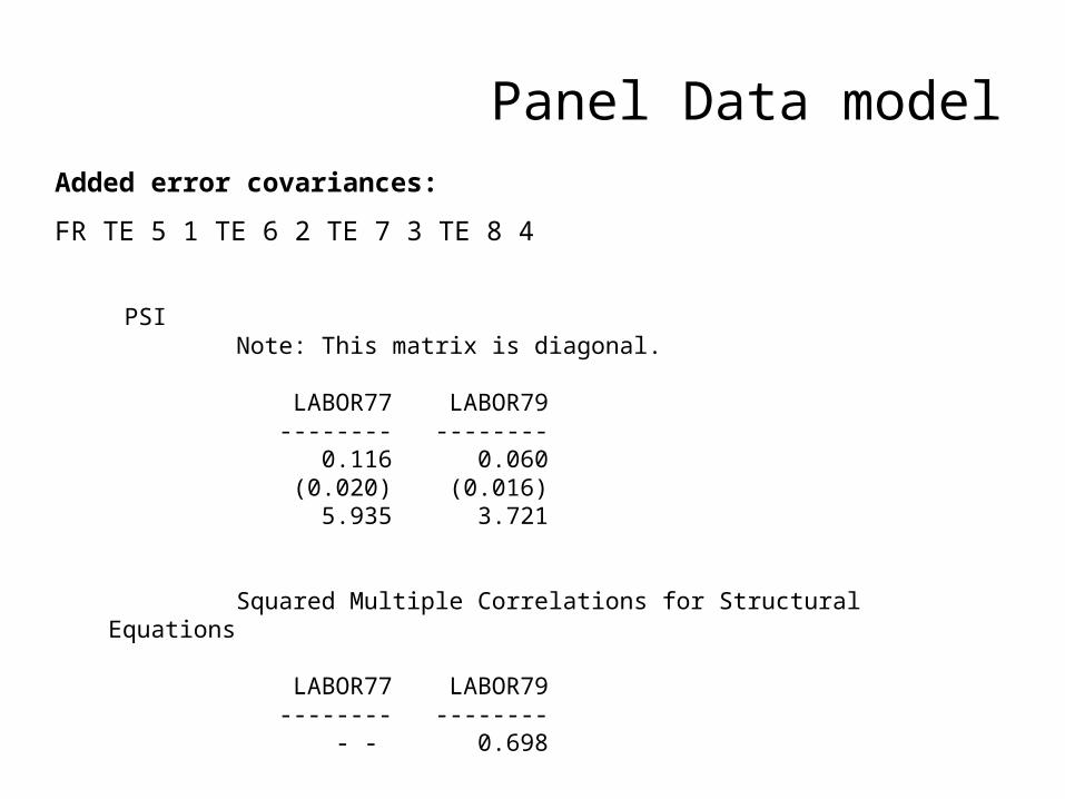
Panel Data model

Added error covariances:

FR TE 5 1 TE 6 2 TE 7 3 TE 8 4

PSI Note: This matrix is diagonal.

LABOR77 LABOR79 -------- -------- 0.116 0.060 (0.020) (0.016) 5.935 3.721

Squared Multiple Correlations for Structural Equations

LABOR77 LABOR79 -------- -------- - - 0.698

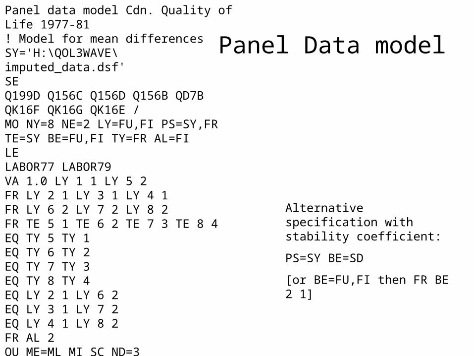
Panel Data model

Panel data model Cdn. Quality of Life 1977-81! Model for mean differencesSY='H:\QOL3WAVE\imputed_data.dsf'SE Q199D Q156C Q156D Q156B QD7B QK16F QK16G QK16E /MO NY=8 NE=2 LY=FU,FI PS=SY,FR TE=SY BE=FU,FI TY=FR AL=FILE LABOR77 LABOR79VA 1.0 LY 1 1 LY 5 2FR LY 2 1 LY 3 1 LY 4 1FR LY 6 2 LY 7 2 LY 8 2 FR TE 5 1 TE 6 2 TE 7 3 TE 8 4EQ TY 5 TY 1EQ TY 6 TY 2EQ TY 7 TY 3EQ TY 8 TY 4EQ LY 2 1 LY 6 2EQ LY 3 1 LY 7 2EQ LY 4 1 LY 8 2FR AL 2OU ME=ML MI SC ND=3

Alternative specification with stability coefficient:

PS=SY BE=SD

[or BE=FU,FI then FR BE 2 1]

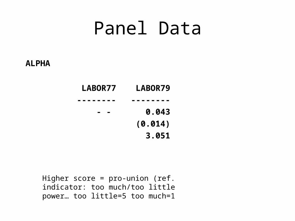
Panel Data

ALPHA

LABOR77 LABOR79

-------- --------

- - 0.043

(0.014)

3.051

Higher score = pro-union (ref. indicator: too much/too little power… too little=5 too much=1

Panel Data

Panel data model Cdn. Quality of Life 1977-81

! Impact of TV newspapers on labor union attitudesSY='H:\QOL3WAVE\imputed_data.dsf'SE Q258 Q260 Q261 Q199D Q156C Q156D Q156B QD7B QK16F QK16G QK16E /MO NY=11 NE=4 LY=FU,FI PS=SY TE=SY BE=FU,FILE NEWSP TV LABOR77 LABOR79VA 1.0 LY 2 1 VA 1.0 LY 3 2FR LY 1 1 FI TE 3 3 VA 1.0 LY 4 3 LY 8 4FR LY 5 3 LY 6 3 LY 7 3FR LY 9 4 LY 10 4 LY 11 4 FR BE 4 3FR BE 3 2 BE 3 1FR BE 4 2 BE 4 1FR PS 2 1 FR TE 11 7 TE 10 6 TE 9 5 TE 8 4OU ME=ML MI SC ND=3

Union Atts1977

1

1111

Union atts1979

1

1111

1

Newsp11

1

TV1

Panel Data

LISREL Estimates (Maximum Likelihood)

LAMBDA-Y

NEWSP TV LABOR77 LABOR79 -------- -------- -------- -------- Q258 0.917 - - - - - - (0.176) 5.212 Q260 1.000 - - - - - - Q261 - - 1.000 - - - - Q199D - - - - 1.000 - - Q156C - - - - -1.891 - - (0.214) -8.819

Panel Data

BETA

NEWSP TV LABOR77 LABOR79 -------- -------- -------- -------- NEWSP - - - - - - - - TV - - - - - - - - LABOR77 0.061 -0.005 - - - - (0.026) (0.011) 2.325 -0.406 LABOR79 0.047 -0.017 1.081 - - (0.030) (0.014) (0.113) 1.584 -1.216 9.564

Panel Data

Panel data model Cdn. Quality of Life 1977-81! Impact of TV newspapers on labor union attitudes! Controls: education sex union membership SY='H:\QOL3WAVE\imputed_data.dsf'SE Q258 Q260 Q261 Q199D Q156C Q156D Q156B QD7B QK16F QK16G QK16E Q63 SEX Q201 RAGE Q157/MO NY=11 NE=4 LY=FU,FI PS=SY TE=SY BE=FU,FI NX=5 NK=5 FIXEDXLE NEWSP TV LABOR77 LABOR79LKMEMBER SEX EDUC AGE INCOMEVA 1.0 LY 2 1 VA 1.0 LY 3 2FR LY 1 1 FI TE 3 3 VA 1.0 LY 4 3 LY 8 4FR LY 5 3 LY 6 3 LY 7 3FR LY 9 4 LY 10 4 LY 11 4 FR BE 4 3FR BE 3 2 BE 3 1FR BE 4 2 BE 4 1FR PS 2 1 FR TE 11 7 TE 10 6 TE 9 5 TE 8 4OU ME=ML MI SC ND=3

Panel Data BETA

NEWSP TV LABOR77 LABOR79 -------- -------- -------- -------- NEWSP - - - - - - - - TV - - - - - - - - LABOR77 -0.025 -0.012 - - - - (0.034) (0.011) -0.738 -1.157 LABOR79 0.068 -0.010 1.033 - - (0.042) (0.013) (0.115) 1.622 -0.751 8.970

GAMMA

MEMBER SEX EDUC AGE INCOME -------- -------- -------- -------- -------- NEWSP -0.017 0.011 -0.097 -0.014 -0.014 (0.039) (0.035) (0.009) (0.001) (0.005) -0.422 0.311 -11.303 -13.496 -2.898 TV -0.013 -0.150 0.025 -0.017 0.001 (0.070) (0.062) (0.015) (0.002) (0.009) -0.182 -2.408 1.685 -9.807 0.113 LABOR77 0.286 -0.056 -0.039 -0.005 -0.010 (0.036) (0.026) (0.008) (0.001) (0.004) 7.880 -2.131 -5.158 -5.331 -2.557 LABOR79 0.045 0.114 0.001 0.001 -0.006 (0.042) (0.033) (0.009) (0.001) (0.004) 1.082 3.487 0.069 0.966 -1.436

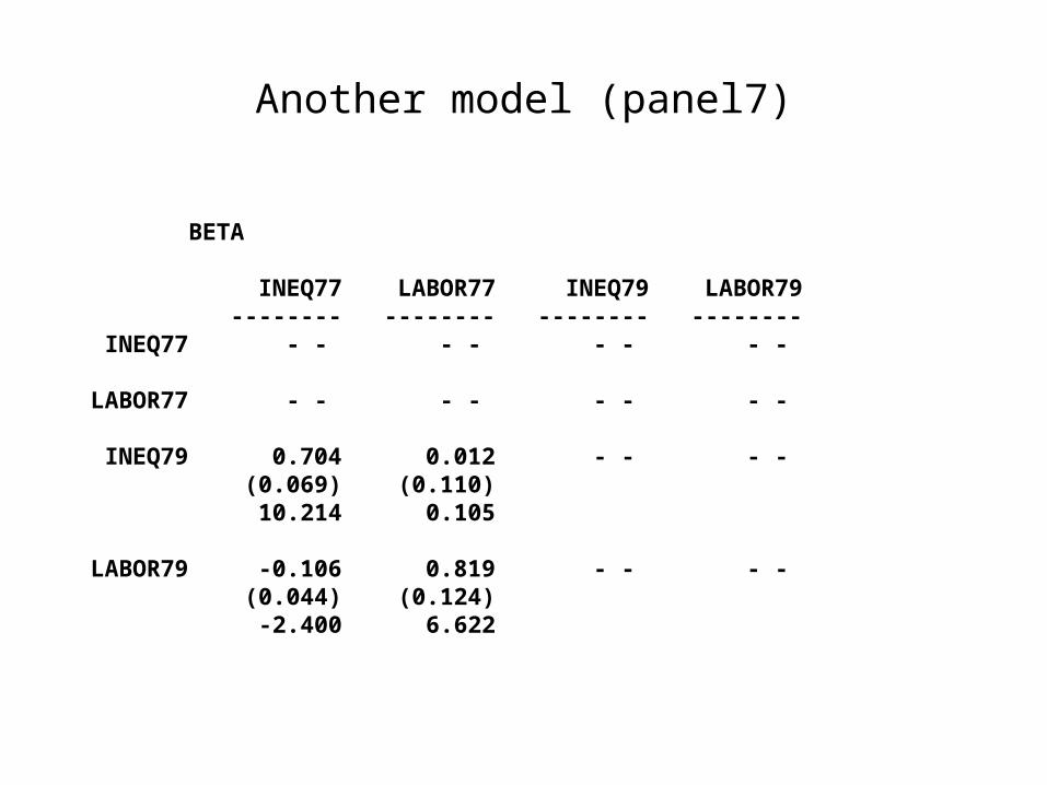
Another model (panel7)

BETA

INEQ77 LABOR77 INEQ79 LABOR79 -------- -------- -------- -------- INEQ77 - - - - - - - - LABOR77 - - - - - - - - INEQ79 0.704 0.012 - - - - (0.069) (0.110) 10.214 0.105 LABOR79 -0.106 0.819 - - - - (0.044) (0.124) -2.400 6.622

Re-expressing parameters:GROWTH CURVE MODELS

Intercept & linear (& sometimes quadratic) terms

• Suitable for panel models with >2 waves

• Best for panel models with >3 waves

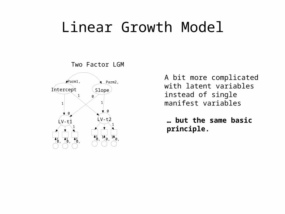
Linear Growth Model

Two Factor LGM

Parm1,

Intercept

Parm2,

Slope

0

V1 - t1

0

V2 - t2

10

1

1

0, 01

0, 01

LISREL:

2 manifest variable, 2 latent variable model

LY matrix

INT Slope

V1 1 0

V2 1 1

TE matrix = elements equal

PS matrix = SY,FR

(parm1 in model = variance of INT, parm2 = variance of Slope)

TY zero

AL free (“parm1” and “parm2” above)

Linear Growth Model

Two Factor LGM

Parm1,

Intercept

Parm2,

Slope

0

V1 - t1

0

V2 - t2

10

1

1

0, 01

0, 01

Interpretation:

• intercept factor represents initial status

•Slope factor represents difference scores (V2-V1)

With single indicators, cannot estimate error variances (as with any single indicator SEM model)

Parm1 = mean intercept Parm2 = mean slope value

Linear Growth Model

Two Factor LGM

Parm1,

Intercept

Parm2,

Slope

0

V1 - t1

0

V2 - t2

10

1

1

0, 01

0, 01

Parm1 = mean intercept Parm2 = mean slope value

E.g., TV use, adolescents, hours/day

Parm1 = 2.5

Parm2 = 1.0

Increase of 1 hour/day from t1 to t2

We will also get variances for the Intercept and the Slope factors

Some growth curve trajectories:

• Parallel stability

Some growth curve trajectories:

• Strict stability

Single-factor LGM

Curve

V1 V2 V3

1 B1 B1

•Actually nested within 2 factor model

• take 2 factor model, intercept with 0 mean and 0 variance or strictly proportional to slope

Not generally the best model unless assumptions met: (cf. Duncan et al. p. 31: when rank ordering of individuals does not vary across time despite mean level changes)

(can estimate var(e1),(e2),(e3) if we impose constraint v(e1)=v(e2)=v(e3) )

Linear Growth Model

Two Factor LGM

Parm1,

Intercept

Parm2,

Slope

0

LV-t1

0,

1

10,1

0,1

0

LV-t2

0,0,0,

1

111

1

01

1

A bit more complicated with latent variables instead of single manifest variables

… but the same basic principle.

Linear Growth ModelTwo Factor Linear Growth Model

Parm1,

Intercept

Parm2,

Slope

0

t1

0

t2

0

t3

11

1 01 2

0,1

0,1

0,1

LY matrix (LISREL)

Int Slope

V1 1 0

V2 1 1

V3 1 2

Same principle would apply to k time points where k>3

More time points: test of linearity of “growth” (changes in mean)*

*general test: vs. “unspecified growth model”

Unspecified 2 factor Growth Curve Model

Two Factor Unspecified Growth Model

Parm1,

Intercept

Parm2,

Slope

0

t1

0

t2

0

t3

11

1 01 lambda

0,1

0,1

0,1

1 free lambda parameter in LY matrix

In k time-point model, all but first 2 time points are represented by free parameters

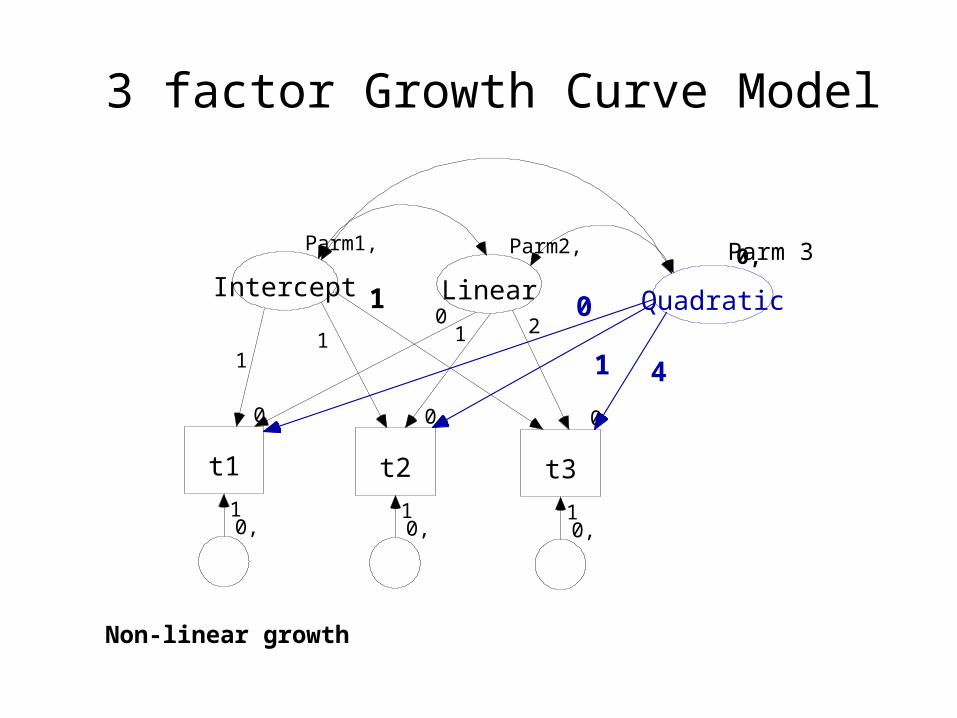
3 factor Growth Curve Model

Parm1,

Intercept

Parm2,

Linear

0

t1

0

t2

0

t3

11

10

1

0,1

0,1

0,1

2

0,

Quadratic0

1 4

Non-linear growth

Parm 3

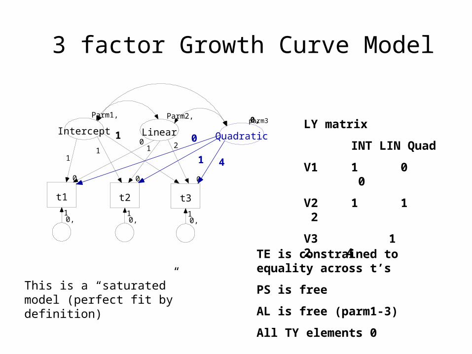
3 factor Growth Curve Model

Parm1,

Intercept

Parm2,

Linear

0

t1

0

t2

0

t3

11

10

1

0,1

0,1

0,1

2

0,

Quadratic0

1 4

LY matrix

INT LIN Quad

V1 1 0 0

V2 1 1 2

V3 1 2 4

TE is constrained to equality across t’s

PS is free

AL is free (parm1-3)

All TY elements 0

parm3

This is a “saturated” model (perfect fit by definition)

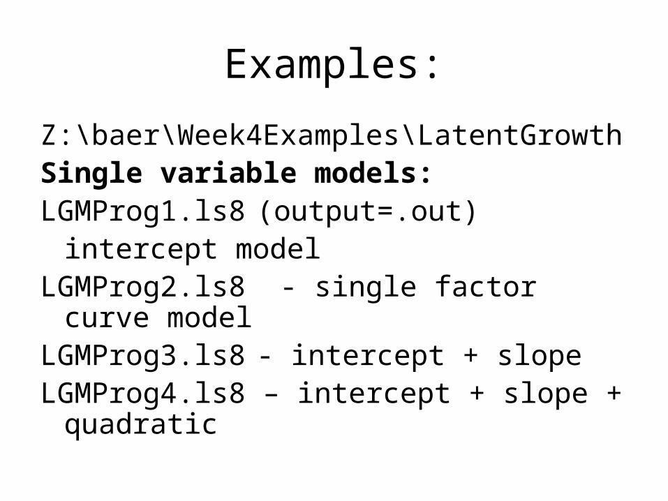
Examples:

Z:\baer\Week4Examples\LatentGrowthSingle variable models:LGMProg1.ls8 (output=.out)

intercept modelLGMProg2.ls8 - single factor curve modelLGMProg3.ls8 - intercept + slopeLGMProg4.ls8 – intercept + slope +

quadratic

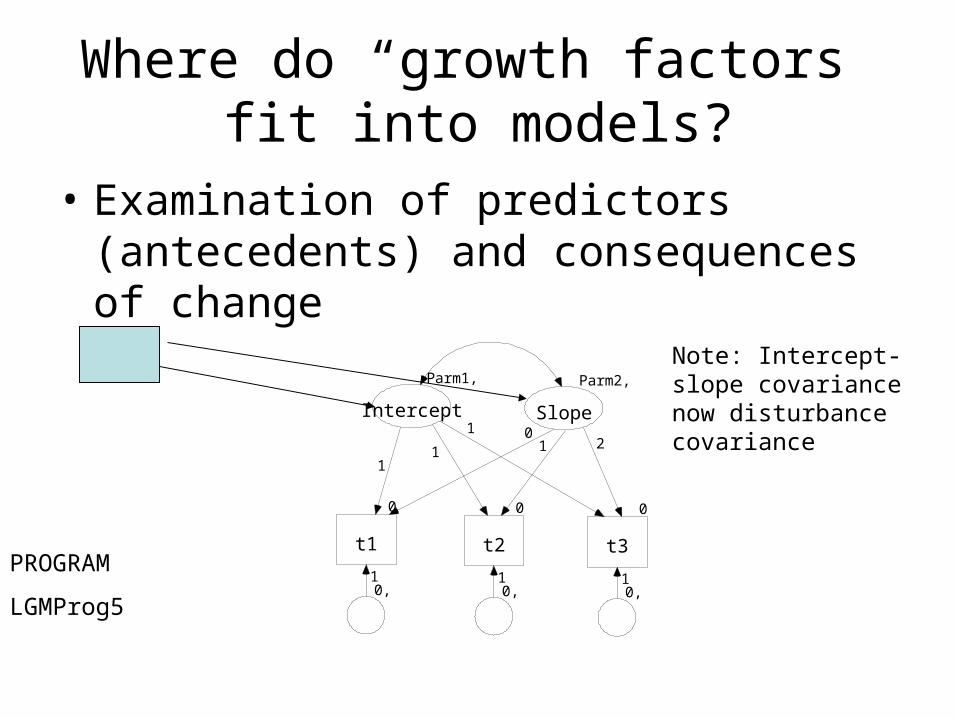
Where do “growth factors” fit into models?

• Examination of predictors (antecedents) and consequences of change

Two Factor Linear Growth Model

Parm1,

Intercept

Parm2,

Slope

0

t1

0

t2

0

t3

11

1 01 2

0,1

0,1

0,1

Note: Intercept-slope covariance now disturbance covariance

PROGRAM

LGMProg5

ConsequencesTwo Factor Linear Growth Model

Parm1,

Intercept

Parm2,

Slope

0

t1

0

t2

0

t3

11

1 01 2

0,1

0,1

0,1

Model LGMProg6.ls8

Dependent variable: job satisfaction, wave 8.

Multiple indicators for the variable(s) involved in growth

curves

• “factor of curves” LGM

• Intercept term and slope term (e.g.) constructed for each indicator

• if there are 3 variables & 4 waves, we will have an intercept term based on 4 manifest variables representing time x 3 manifest variables per time (3 intercept terms)

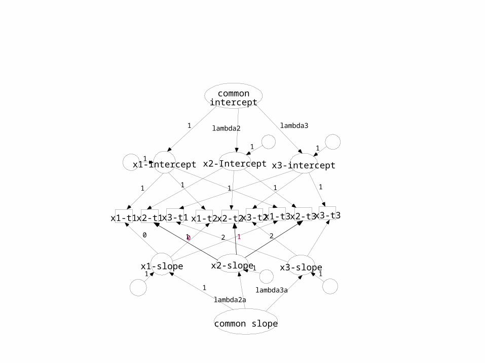
“common intercept” variable will have 3 indicators (intercept terms)

“common slope” will have 3 indicators (slope terms)

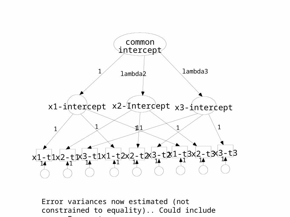
x1-intercept

x2-t11

x1-t1 x3-t11

x2-t2x1-t2 x3-t21 11 1

x2-t3x1-t3 x3-t31 11

1

x2-Intercept

1 1

x3-intercept

11 1 1

commonintercept

1 lambda2 lambda3

Error variances now estimated (not constrained to equality).. Could include corr. Errors too

x1-intercept

x2-t2x1-t2 x3-t2 x2-t3x1-t3 x3-t3

x2-Intercept

1

x3-intercept

1 1

commonintercept

1 lambda2 lambda3

x3-t1x2-t1x1-t1

1 1

x1-slope x2-slope x3-slope

common slope

0 1 20 1 2

lambda2a

1 lambda3a

1

1 1

11

1

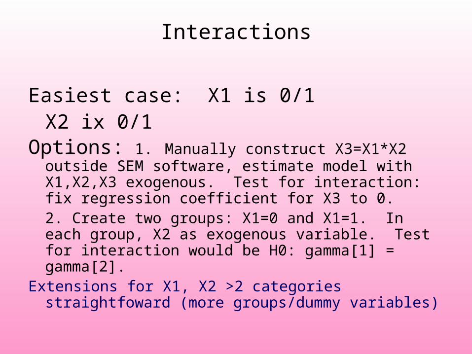
Interactions

Easiest case: X1 is 0/1X2 ix 0/1

Options: 1. Manually construct X3=X1*X2 outside SEM software, estimate model with X1,X2,X3 exogenous. Test for interaction: fix regression coefficient for X3 to 0.2. Create two groups: X1=0 and X1=1. In each group, X2 as exogenous variable. Test for interaction would be H0: gamma[1] = gamma[2].

Extensions for X1, X2 >2 categories straightfoward (more groups/dummy variables)

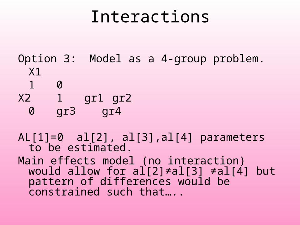
Interactions

Option 3: Model as a 4-group problem.X11 0

X2 1 gr1 gr20 gr3 gr4

AL[1]=0 al[2], al[3],al[4] parameters to be estimated.

Main effects model (no interaction) would allow for al[2]≠al[3] ≠al[4] but pattern of differences would be constrained such that…..

Interactions

Model as a 4-group problem.X11 0

X2 1 gr1 gr20 gr3 gr4

AL[1]=0 al[2], al[3],al[4] parameters to be estimated.Main effects model (no interaction) would allow for al[2]≠al[3] ≠al[4] but pattern

of differences would be constrained such that…..

The group1 vs. group 2 difference = group 3 vs. group 4 difference(or group 1 vs. 3 difference = group 2 vs. group 4).Programming in LISREL would be:Al[1] – Al[2] = al[3]- al[4]0 – al[2] = al[3] – al[4] Al[2] = al[4]-al[3] LISREL: CO al 2 1 = al 4 1 – al 3 1 Test for interaction: run another model removing this constraint (all AL

completely free except group 1)

… more examples provided in text

Interactions

Interactions involving continuous variables.

Case 1: One continuous (single or multiple indicator) and one categorical variableEASY: categorical variable becomes basis for grouping.

Group 1 Eta = gamma[1] Ksi + zetaGroup 2 Eta = gamma[2] Ksi + zetaTest for interaction: H0: gamma[1] = gamma[2]

Case 2: Two continuous single indicator variablesAlso somewhat straightforward:

Create single-indicator X3 = X2*X1

Case 3: Two continuous multiple indicator latent variablesThis is not so easy! Substantial literature on this question See course outline for extended list. (Schumacker and Mracoulides, eds., Interaction and Nonlinear Effects in Structural Equation Modeling).

Case 3A, not talked about much: X1 single indicator Ksi1 (X2, X3,X4)Create: X1X2 , X1X3, X1,X4

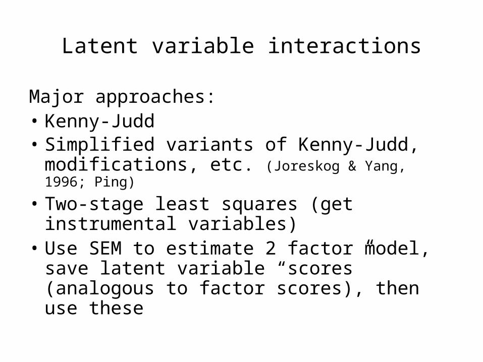
Latent variable interactions

Major approaches:• Kenny-Judd• Simplified variants of Kenny-Judd,

modifications, etc. (Joreskog & Yang, 1996; Ping)

• Two-stage least squares (get instrumental variables)

• Use SEM to estimate 2 factor model, save latent variable “scores” (analogous to factor scores), then use these

Latent variable interactions

• Use SEM to estimate 2 factor model, save latent variable “scores” (analogous to factor scores), then use these

In LISREL:

Mo nx=6 nk=2 lx=fu,fi ph-sy,fr td=sy

Va 1.0 lx 1 1 lx 4 2

Fr lx 2 1 lx 3 1 lx 5 2 lx 6 2

PS=Newfile.psf

OU

Latent variable interactions• Use SEM to estimate 2 factor model, save latent variable “scores”

(analogous to factor scores), then use these

In LISREL:

Mo nx=6 nk=2 lx=fu,fi ph-sy,fr td=sy

Va 1.0 lx 1 1 lx 4 2

Fr lx 2 1 lx 3 1 lx 5 2 lx 6 2

PS=Newfile.psf

OU

LISREL documentation suggests that a simple regression can be estimated in PRELIS:

Sy=newfile.psf

ne inter=ksi1*ksi2

rg y on ksi1 ksi2 ksi1 ksi2

ou

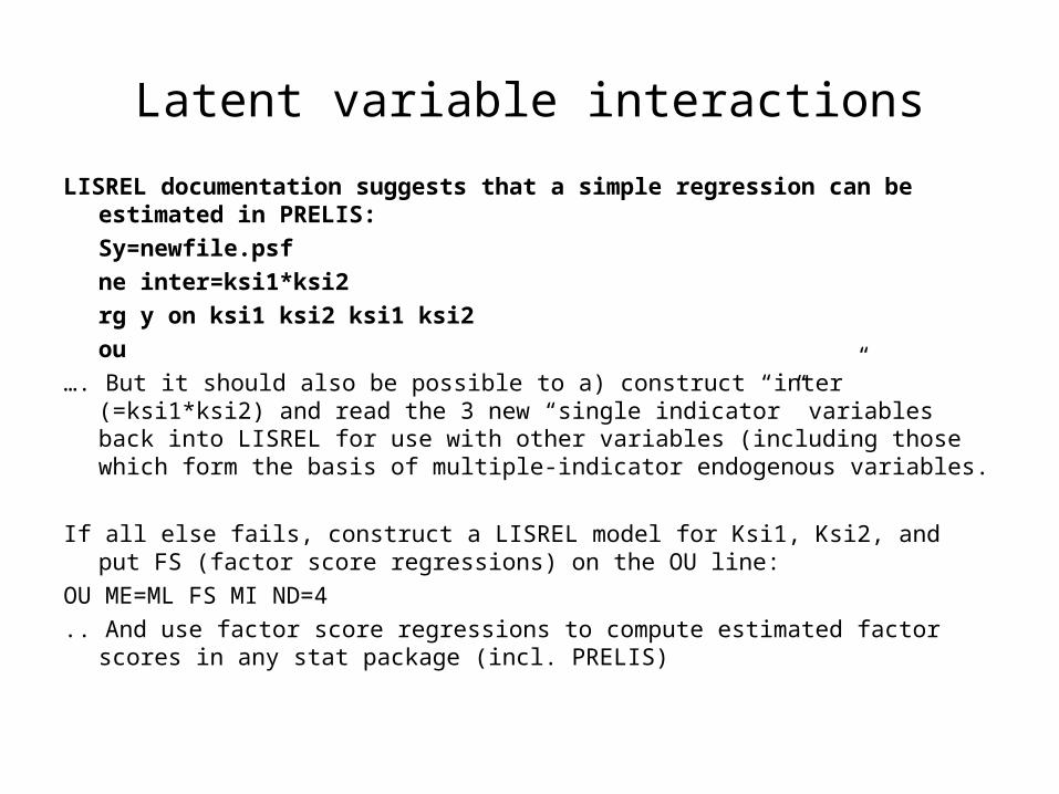
Latent variable interactions

LISREL documentation suggests that a simple regression can be estimated in PRELIS:

Sy=newfile.psf

ne inter=ksi1*ksi2

rg y on ksi1 ksi2 ksi1 ksi2

ou

…. But it should also be possible to a) construct “inter” (=ksi1*ksi2) and read the 3 new “single indicator” variables back into LISREL for use with other variables (including those which form the basis of multiple-indicator endogenous variables.

If all else fails, construct a LISREL model for Ksi1, Ksi2, and put FS (factor score regressions) on the OU line:

OU ME=ML FS MI ND=4

.. And use factor score regressions to compute estimated factor scores in any stat package (incl. PRELIS)

Example:INTERACTION MODEL WITH INTERACTION TERM CREATED EXTERNALLY SINGLE INDICATORS FOR EXOGENOUS LVS INVOLVED IN INTERACTION DA NO=1111 NI=10 MA=CM CM FI=G:\ICPSR\INTERACTIONS\INT5b.COV FU FO (10F10.7) LABELS lv1 lv2 interact sex race v217 v216 v125 v127 v130 se 8 9 10 1 2 3 4 5 6 7/ mo ny=3 ne=1 LY=FU,FI PS=SY,FR TE=SY c nx=7 nk=7 fixedx ga=fu,fr va 1.0 ly 1 1 fr ly 2 1 ly 3 1 ou me=ml se tv mi sc

Example:LISREL Estimates (Maximum Likelihood)

LAMBDA-Y

ETA 1 -------- v125 1.00 v127 1.34 (0.24) 5.59 v130 0.65 (0.11) 5.74

GAMMA

lv1 lv2 interact sex race v217 -------- -------- -------- -------- -------- -------- ETA 1 -0.04 -0.21 0.85 0.22 -0.30 0.05 (0.06) (0.08) (0.45) (0.11) (0.13) (0.03) -0.65 -2.57 1.89 2.10 -2.27 1.75

GAMMA

v216 -------- ETA 1 0.09 (0.03) 2.92

Dep var = inequality att’s (high score “more individual effort”)

Lv1=relig. Lv2=econ. status

Kenny-Judd model

Typically, literature (e.g., Kenny-Judd, 1984; Hayduk, 1987) starts with 2-indicator example (2 LV’s each with 2 indicators).

Ksi1

Ksi2 Ksi1*Ksi2 (interaction term)

Indicators: Ksi1: x1

x2

Ksi2: x3

x4

Possible product terms:

x1*x3 x1*x4

x2*X3 X2*x4

Kenny-Judd model use 4 product terms but Joreskog and Yang show that the model can be constructed with 1 product term.

Kenny-Judd model

Typically, literature (e.g., Kenny-Judd, 1984; Hayduk, 1987) starts with 2-indicator example (2 LV’s each with 2 indicators).

Ksi1

Ksi2 Ksi1*Ksi2 (interaction term)

Indicators: Ksi1: x1

x2

Ksi2: x3

x4

Possible product terms:

x1*x3 x1*x4

x2*X3 X2*x4

Kenny-Judd model use 4 product terms but Joreskog and Yang show that the model can be constructed with 1 product term.

Kenny-Judd do not include constant intercept terms (alpha, tau).. But even if dependent variable, Ksi1, Ksi2 and zeta have zero means, alpha will still be nonzero. - means of observed variables functions of other parameters in the model and therefore intercept terms have to be included.

- Nonnormality even if x’s are normal (ADF estimation often recommended if sample size acceptable)

Kenny-Judd model

Kenny-Judd model

alpha=1 term

Kenny-Judd model, mod.INTERACTION MODEL KENNY JUDD MODIFICATION (JORESKOG AND YANG) ONE INTERACTION INDICATOR 3 INDICATORS PER L.V. DA NO=1111 NI=22 CM FI=G:\ICPSR2000\INTERACTIONS\INT5c.COV FU FO (22F20.11) ME FI=G:\ICPSR2000\INTERACTIONS\INT5C.MN FO (22F20.11) LABELS v181 v9 v190 v221 v226 v227 relinc1 relinc2 relinc3 relinc4 relinc5 relinc6 relinc7 relinc8 reling9 sex race v217 v216 v125 v127 v130 se 20 21 22 1 2 3 4 5 6 9 16 17 18 19/ mo ny=3 ne=1 NX=11 NK=7 LY=FU,FI PS=SY,FR C TE=SY TX=FR KA=FI C LX=FU,FI GA=FU,FR PH=SY,FR TD=SY AL=FI TY=FR va 1.0 ly 1 1 fr ly 2 1 ly 3 1 FI PH 3 1 PH 3 2 FR KA 3 VA 1.0 LX 1 1 LX 4 2 LX 7 3 LX 8 4 LX 9 5 LX 10 6 LX 11 7 FR TD 1 1 TD 2 2 TD 3 3 TD 4 4 TD 5 5 TD 6 6 TD 7 7 FR LX 2 1 LX 3 1 LX 5 2 LX 6 2 LX 7 1 LX 7 2 CO LX(7,1)=TX(1) CO LX(7,2)=TX(4) CO KA(3) = PH(2,1) FI PH 3 1 PH 3 2 CO PH(3,3) = PH(1,1)*PH(2,2) + PH(2,1)**2 CO TX(6) = TX(1)*TX(4) FI TD(8,8) TD(9,9) TD(10,10) TD(11,11) CO TD(7,7) = TX(1)**2*TD(3,3) + TX(4)**2*TD(1,1) + PH(1,1)*TX(4) + C PH(2,2)*TX(1) + TD(1,1)*TD(4,4) OU ME=ML SE TV ND=3 AD=off

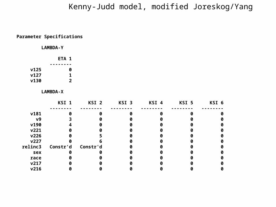
Kenny-Judd model, modified Joreskog/Yang

Parameter Specifications

LAMBDA-Y

ETA 1 -------- v125 0 v127 1 v130 2

LAMBDA-X

KSI 1 KSI 2 KSI 3 KSI 4 KSI 5 KSI 6 -------- -------- -------- -------- -------- -------- v181 0 0 0 0 0 0 v9 3 0 0 0 0 0 v190 4 0 0 0 0 0 v221 0 0 0 0 0 0 v226 0 5 0 0 0 0 v227 0 6 0 0 0 0 relinc3 Constr'd Constr'd 0 0 0 0 sex 0 0 0 0 0 0 race 0 0 0 0 0 0 v217 0 0 0 0 0 0 v216 0 0 0 0 0 0

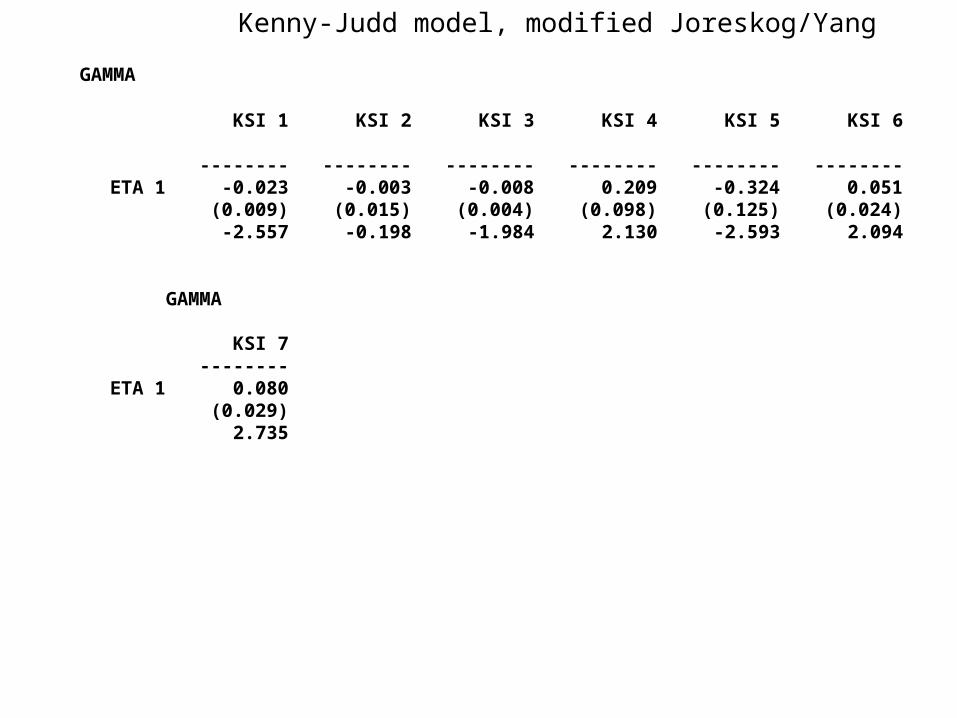
Kenny-Judd model, modified Joreskog/Yang

GAMMA

KSI 1 KSI 2 KSI 3 KSI 4 KSI 5 KSI 6 -------- -------- -------- -------- -------- -------- ETA 1 -0.023 -0.003 -0.008 0.209 -0.324 0.051 (0.009) (0.015) (0.004) (0.098) (0.125) (0.024) -2.557 -0.198 -1.984 2.130 -2.593 2.094

GAMMA

KSI 7 -------- ETA 1 0.080 (0.029) 2.735