Icp Appendix
55
Chemical Properties 04.14 Appendix Test Methods for the Examination of Composting and Compost March 20, 2001 04.14–1 APPENDIX TO TMECC SECTION 04.14—ICP ANALYSIS AUTHORS OF ICP ANALYSIS—PARVIZ N. SOLTANPOUR; Colorado State University; Fort Collins, Colorado; GREG W. JOHNSON; Matheson Gas Products; Longmont, Colorado; STEPHEN M. WORKMAN; Analytical Technologies, Inc.; Fort Collins, Colorado; J. BENTON JONES, JR.; Macro-Micro Analytical Services; Athens, Georgia; ROBERT O. MILLER; Colorado State University, Fort Collins, Colorado. 1. Introduction 1.1 ICP-AES and ICP-MS. ICP is generally superior in accuracy, precision, detection limit, freedom from interferences, and dynamic range than other analytical instrumentation. The use of automatic samplers, large computers, and appropriate software facilitates accurate and rapid analysis. One can analyze a solution for many elements in 1 min (ICP-AES); therefore, large volumes of data can be generated very fast. Isaac and Johnson (1982) indicate that with ICP-AES one technician can do the same work that formerly required four technicians. Thought should be given to the handling and processing of the data. Interfacing the instrument with larger computers for data handling and analysis is a must if one contemplates obtaining large volumes of data. It is recommended that users of ICP-AES and ICP-MS subscribe to the ICP-Information Newsletter (Department of Chemistry, University of Massachusetts, Amherst) and other newsletters available from the manufacturer of their unit so that they can be kept abreast of new developments in ICP-AES and ICP-MS. Journals such as Applied Spectroscopy, Analytical Chemistry, Analytical Chimica Acta, and others referred to in this chapter are also good sources of information. Additional sources of information have been described in the text. 1.2 Inductively coupled plasma (ICP) analysis is applied to nitric acid digests after digestion by the US EPA Method 3051, Microwave Assisted Digestion and SW-846 US EPA Method 3050A. Wet digestion is performed on an air-dried sample (36°C). 1.2.1 Volatile loss of As and Hg will occur at higher temperatures, (e.g. > 36°C). Mercury determination may be performed on a subsample of the EPA-3051 digest with the cold vapor atomic absorption method. 1.2.2 The measured data are adjusted and reported on a oven dried 70±5°C basis. Elemental determinations are for Ca, Mg, Na, K, P, Fe, Mn, Al, Cu, Zn, Cd, Cr, Ni, Pb, Mo, As, and B. Optional elements available: Ba, Be, Co, Li, Rb, Si, Sr, S, Ti, and V. 1.3 ICP-AES and ICP-MS Instrumentation—The ICP is produced by passing initially ionized Ar gas through a quartz torch located inside a Cu coil connected to a radio frequency (RF) generator. The RF generator provides up to 3 kW forward power (in most commercial units) at a frequency of 27.1 MHz. The high-frequency currents flowing in the Cu coil generate oscillating magnetic fields whose lines of force are axially oriented inside the quartz tube and follow elliptical closed paths outside the coil (Fassel, 1977; Fassel and Kniseley, 1974). Electrons and ions passing through the oscillating electromagnetic field flow at high acceleration rates in closed annular paths inside the quartz tube space. The induced magnetic fields direction and strength vary with time resulting in electron acceleration on each half cycle. Collisions between accelerated electrons and ions, and ensuing unionized Ar gas cause further ionization. 1.3.1 The collisions cause ohmic heating and, when measured spectroscopically, give thermal temperatures ranging from 6,000 to 10,000 °K (Fassel, 1977). However, with the advent of the ICP-MS, it is evident that the true thermal temperature of the plasma is much lower than this. For example, the Perkin Elmer SCIEX 500 that has been in the DANR Analytical Lab for over a year, has run for hours with the "6000 °K" region of the plasma striking the copper interface plate with no melting or etching of the copper metal surface. In addition, several ICP-MS laboratories use copper as the sampler cone metal (Hieftje and Vickers, 1989; Houk, 1986). Copper appears to give satisfactory results in this role unless sulfuric acid is present in the test solutions and the sampler cone aperture is relatively small (i.e. cf. 0.4 mm); in which case, rapid erosion has been observed (Munro et al., 1986). Copper metal melts at 1356°K and boils at 2840°K (Weast and Astle, 1979). 1.3.2 The quartz torch has three concentric channels. The outer channel conducts Ar gas at about 15 L min -1 to 17 L min -1 to the plasma to sustain the plasma and to isolate the quartz tube from high temperatures. The innermost channel is for introduction of sample into the plasma. The middle channel conducts the auxiliary Ar gas at about 1 L -1 min -1 and is used in ICP-AES only when starting the plasma or for organic samples, and is routinely used for all types of samples for ICP-MS. The ICP has an annular, or donut, shape when it is viewed from above. The hole has a lower temperature than the donut body and offers less resistance to the sample injection. The sample is injected into the plasma by using Ar carrier gas at a rate of about 1 L -1 min -1 for ICP-AES work. For ICP-MS work the aerosol flow is approximately 1.5 L min -1 . 1.4 Properties of ICP—The ICP generated, as discussed above, has unique physical properties that make it an excellent source for
-
Upload
karthikeyan-jagannathan -
Category
Documents
-
view
230 -
download
4
Transcript of Icp Appendix

Chemical Properties04.14 Appendix
Test Methods for the Examination of Composting and Compost March 20, 200104.14–1
APPENDIX TO TMECC SECTION 04.14—ICP ANALYSIS
AUTHORS OF ICP ANALYSIS—PARVIZ N. SOLTANPOUR; Colorado State University; Fort Collins, Colorado; GREG W. JOHNSON;Matheson Gas Products; Longmont, Colorado; STEPHEN M. WORKMAN; Analytical Technologies, Inc.; Fort Collins, Colorado; J.BENTON JONES, JR.; Macro-Micro Analytical Services; Athens, Georgia; ROBERT O. MILLER; Colorado State University, Fort Collins,Colorado.
1. Introduction
1.1 ICP-AES and ICP-MS. ICP is generally superiorin accuracy, precision, detection limit, freedom frominterferences, and dynamic range than other analyticalinstrumentation. The use of automatic samplers, largecomputers, and appropriate software facilitates accurateand rapid analysis. One can analyze a solution for manyelements in 1 min (ICP-AES); therefore, large volumesof data can be generated very fast. Isaac and Johnson(1982) indicate that with ICP-AES one technician cando the same work that formerly required fourtechnicians. Thought should be given to the handlingand processing of the data. Interfacing the instrumentwith larger computers for data handling and analysis is amust if one contemplates obtaining large volumes ofdata. It is recommended that users of ICP-AES andICP-MS subscribe to the ICP-Information Newsletter(Department of Chemistry, University of Massachusetts,Amherst) and other newsletters available from themanufacturer of their unit so that they can be keptabreast of new developments in ICP-AES and ICP-MS.Journals such as Applied Spectroscopy, AnalyticalChemistry, Analytical Chimica Acta, and others referredto in this chapter are also good sources of information.Additional sources of information have been describedin the text.
1.2 Inductively coupled plasma (ICP) analysis isapplied to nitric acid digests after digestion by the USEPA Method 3051, Microwave Assisted Digestion andSW-846 US EPA Method 3050A. Wet digestion isperformed on an air-dried sample (36°C).
1.2.1 Volatile loss of As and Hg will occur at highertemperatures, (e.g. > 36°C). Mercury determinationmay be performed on a subsample of the EPA-3051digest with the cold vapor atomic absorption method.
1.2.2 The measured data are adjusted and reported ona oven dried 70±5°C basis. Elemental determinationsare for Ca, Mg, Na, K, P, Fe, Mn, Al, Cu, Zn, Cd, Cr,Ni, Pb, Mo, As, and B. Optional elements available:Ba, Be, Co, Li, Rb, Si, Sr, S, Ti, and V.
1.3 ICP-AES and ICP-MS Instrumentation—The ICPis produced by passing initially ionized Ar gas through aquartz torch located inside a Cu coil connected to aradio frequency (RF) generator. The RF generatorprovides up to 3 kW forward power (in mostcommercial units) at a frequency of 27.1 MHz. Thehigh-frequency currents flowing in the Cu coil generate
oscillating magnetic fields whose lines of force areaxially oriented inside the quartz tube and followelliptical closed paths outside the coil (Fassel, 1977;Fassel and Kniseley, 1974). Electrons and ions passingthrough the oscillating electromagnetic field flow at highacceleration rates in closed annular paths inside thequartz tube space. The induced magnetic fieldsdirection and strength vary with time resulting inelectron acceleration on each half cycle. Collisionsbetween accelerated electrons and ions, and ensuingunionized Ar gas cause further ionization.
1.3.1 The collisions cause ohmic heating and, whenmeasured spectroscopically, give thermal temperaturesranging from 6,000 to 10,000 °K (Fassel, 1977).However, with the advent of the ICP-MS, it is evidentthat the true thermal temperature of the plasma is muchlower than this. For example, the Perkin Elmer SCIEX500 that has been in the DANR Analytical Lab for overa year, has run for hours with the "6000 °K" region ofthe plasma striking the copper interface plate with nomelting or etching of the copper metal surface. Inaddition, several ICP-MS laboratories use copper as thesampler cone metal (Hieftje and Vickers, 1989; Houk,1986). Copper appears to give satisfactory results inthis role unless sulfuric acid is present in the testsolutions and the sampler cone aperture is relativelysmall (i.e. cf. 0.4 mm); in which case, rapid erosion hasbeen observed (Munro et al., 1986). Copper metal meltsat 1356°K and boils at 2840°K (Weast and Astle, 1979).
1.3.2 The quartz torch has three concentric channels.The outer channel conducts Ar gas at about 15 L min-1
to 17 L min-1 to the plasma to sustain the plasma and toisolate the quartz tube from high temperatures. Theinnermost channel is for introduction of sample into theplasma. The middle channel conducts the auxiliary Argas at about 1 L-1 min-1 and is used in ICP-AES onlywhen starting the plasma or for organic samples, and isroutinely used for all types of samples for ICP-MS. TheICP has an annular, or donut, shape when it is viewedfrom above. The hole has a lower temperature than thedonut body and offers less resistance to the sampleinjection. The sample is injected into the plasma byusing Ar carrier gas at a rate of about 1 L-1 min-1 forICP-AES work. For ICP-MS work the aerosol flow isapproximately 1.5 L min-1.
1.4 Properties of ICP—The ICP generated, asdiscussed above, has unique physical properties thatmake it an excellent source for

vaporization/atomization/ionization/excitation ofelements.
1.4.1 Method 04.14–A Inductively Coupled Plasma-Atomic Emission Spectroscopy, US EPA Method6010A—the aerosol droplets containing the analyte aredesolvated, the analyte salts/oxides are vaporized, andthe analyte atomized at the high temperature region ofthe plasma in the vicinity of the Cu coil. An initialradiation zone (IRZ) has been defined by Koirtyohann etal. (1980) as the zone that begins in the sample aerosolchannel inside the load coil for ICP-AES. The IRZextends upward to one or two mm above the load coil,taking on the appearance of an amber "bullet" duringnebulization of many sample types related to agriculture.This is due to emission from CaO molecules on thesurface of the "bullet", the color changing to a deep blueor purple further downstream as emission from calciumatoms and ions dominates. The blue/purple region istermed the normal analytical zone (NAZ), and is theregion in which the analyte emission is observed by thespectrometer. Color photographs illustrating theappearance of the IRZ and NAZ while nebulizing anelevated concentration of yttrium into an ICP haverecently been published for ICP-AES (Winge et al.,1988), and more clearly define these critical regions.The NAZ is 15- to 20-mm above the coil, or about 14-to 19-mm above the tip of the IRZ, in an environmentrelatively low in background emission. The backgroundconsists of Ar lines and some weak band emission fromOH, NO, and CN molecules present in the plasma(Ward, 1978a). By the time the decomposition productsof the sample reach the NAZ, they have had a residencetime of about 2 msec at spectroscopically measuredtemperatures ranging from about 8,000 to 5,000 °K(Fassel, 1977). The residence time and temperatureexperienced by samples introduced into the plasmas areabout twice as large as those in the hottest flames, e.g.,N2O-C2H2. The high temperature and residence timecombination, at the sample aerosol flow rates typicallyused in ICP-AES, lead to complete sample vaporizationand atomization in contrast to flames that requirereleasing agents for refractory compounds (Larson et al.,1975). Once the free compounds, atoms, and ions areformed in ICP-AES, they are in a chemically inertenvironment in contrast to highly reactive combustionflame environments. Ionization interferences aregenerally negligible in an ICP-AES experiment. Self-absorption (a phenomenon responsible for the flatteningof the standard curve at high analyte concentrations) ispractically absent, which leads to a wide linear dynamicanalytical range of 3 to 5 decades. No sampling orskimmer cones, and lense stack or quadrupole rods areused in the ICP-AES, and therefore, contamination fromablative processes off of them, e.g. secondary ionsputtering, is absent.
1.4.2 ICP-MS—the vaporization and atomizationbegin at approximately the same location relative to theload coil as do these processes in the ICP-AES, in arelatively hot region of the plasma in the vicinity of theCu coil. However, the flow rates of sample and/orauxiliary argon are increased for ICP-MS to obtain ananalytically useful population of ions (Winge, et al.,1991), while keeping the sampling cone a safe distancefrom the load Cu coil to prevent arcing between the coneand the load cu coil. The IRZ extends well beyond thedownstream side of the load cu coil. The water dropletsproduced in a conventional concentric nebulizer,although apparently extremely few in number comparedto the total number of aerosol droplets produced, cansurvive the rigorous desolvation/atomization conditionsgenerated by the ICP (Winge et al., 1991). Although thedownstream side of the load coil-to-IRZ tip distancevaries from one lab to another, it is generally between10 and 20 mm for ICP-MS. Unlike ICP-AES, thisleaves much of the analyte vaporization and atomizationto be done in regions beyond the hottest parts of the ICPin the ICP-MS case. The sampling cone orifice definesthe NAZ in the ICP-MS, and is another 2- to 10-mmdownstream from the tip of the IRZ. In the DANRAnalytical Lab, the IRZ extends approximately 19 mmdownstream from the spectrometer side of the load coiland the sampler cone orifice is positioned another 3 mmdownstream from the IRZ tip; which results inplacement of the NAZ a total of 22 mm from the nearestsurface of the load coil. Most of the particle beam issucked through the sampling cone into the intermediatevacuum region of a differentially pumped apertureapproximately two to three mm from the tip of thebullet. The tip of a second cone, called the skimmer, isimmersed in what is termed a barrel shock (Gray, 1989)that results from supersonic expansion of the plasma gasas it passes from atmospheric pressure through thesampling cone orifice into a vacuum of about 1 torr.The kinetic temperature of the gaseous particles at thetip of the skimmer cone has been measured to be 2200"K (Lim et al., 1989; Winge, et al., 1991). Although theposition of the sampler with respect to the extended IRZof the ICP results in a maximum rate of ions per secondat the detector, it also is sampling aerosol that hasundergone solute vaporization and atomization reactionsoutside the hottest regions of the ICP. This is thought tocontribute to the appearance of more molecular ions inthe mass spectra and higher susceptibility to non-spectroscopic matrix effects than if the aerosol flow rateand/or auxiliary argon flow rate could be slowed downenough to put the IRZ back to within one or two mm ofthe downstream side of the load coil. However, this isnot possible because of the arcing that occurs betweenthe load coil and the metallic sampling cone in instancesin which the cone is placed too close spatially to theload coil. We have been unsuccessful at locatingdescriptions of ICP-MS experiments designed to reduce

Chemical Properties04.14 Appendix
Test Methods for the Examination of Composting and Compost March 20, 200104.14–3
molecular ion formation in the mass spectrum using asampler constructed of a sampling cone that does notconduct electricity. Among the possibilities for non-conducting materials are high tech ceramics that couldwithstand prolonged exposure to the highest temperatureregions of the ICP. These include AlN, SiC, Al2O3, orzirconia ceramics1. The sampler could be placed so thatthe NAZ is in a region closer to local thermodynamicequilibrium (LTE) with respect to maximized ionpopulations while the analyte solute vaporization andatomization is allowed to proceed in the hottest parts ofthe plasma.
1.5 Normal Analytical Zone—In general, the normalanalytical zone (NAZ) is much closer to the tip of theIRZ in ICP-MS (2 to 10 mm) than the NAZ is to the tipof the IRZ in ICP-AES (14 to 19 mm). The closerproximity used for the ICP-MS measurements increasesthe concentration of ions to a level at which they areanalytically useful (Winge et al.., 1991). Ideally, ionsshould be extracted from a region that approximateslocal thermal equilibrium (LTE). Apparently, iontemperatures are sufficient to support high ionpopulations at this proximity to the IRZ tip.Undoubtedly, the requirement for high ion density at adistance well downstream from maximum gas andexcitation temperatures promotes formation of metaloxide ions and non-spectroscopic concomitantsuppression effects that are observed in the ICP-MS. Anumber of modifications that will be mentioned below,most involving the usual sample introductiontechniques, have been found to significantly reducethese problems.
2. Application
2.1 The application of inductively coupled plasma-atomic emission spectrometry (ICP-AES) to the analysisof soil was reviewed in 1982 and again in 1996 withinclusion of ICP-mass spectrometry (ICP-MS),(Soltanpour, et al., 1982 and 1996). The main objectiveof this review is to treat ICP-MS more comprehensivelywith inclusion of a table for isotopes of elements (seeselection of isotopes section in 04.14 Appendix) and anexample for Ca, Fe, Ni, Zn and Pb isotope selection forplant tissue analysis (04.14 Appendix).
2.1.1 TMECC Method 04.14–A Inductively CoupledPlasma-Atomic Emission Spectroscopy, US EPAMethod 6010A—New developments in ICP-AESinclude: suspension nebulization analysis of clays (Lairdet al., 1991); interfacing ICP spectrometers with flowinjection analyzers for automatic dilution, calibration,separation, concentration, standard additions and otheroperations (Greenfield, 1983; LaFerniere, et al., 1985);interfacing ICP-AES with liquid chromatographs for
1 Coors Ceramics, 9th and Ford Street, Golden, CO
concentration and speciation of elements(Roychowdhury and Koropchack, 1990); high saltnebulizers to prevent clogging of nebulizers (Legere andBurgener, 1985); successful use of concentration andreduction of spectral interferences techniques such aschelation/ solvent extraction (Huang and Wai, 1986;Bradford and Bakhtar, 1991); use of computer programssuch as orthogonal polynomials (Hassan and Loux,1989), simplex optimization (Belchamber et al., 1986),and that recommended by Taylor and Schutyser, 1986,for optimization of spectrometer operating conditionsand automatic correction for spectral interferences; andcompilation of ICP emission lines still in progress(McLaren and Berman, 1985; Boumans, 1984; andParsons et al, 1980).
2.1.2 ICP-MS—This method of analysis has beendeveloped over the last fifteen years. Houk, et al., 1981showed suprathermal ionization in an ICP argon plasma.Within the last ten years it has become possible to applythe method to routine analytical concentrationdeterminations. Several review articles document theICP-MS developmental milestones (Beauchemin, 1989;Hieftje and Vickers, 1989; Douglas, 1989; Houk andThompson, 1988; Houk, 1986; Gray, 1985; Douglas andHouk, 1985). Between 1986 and 1988, ICP-MSenjoyed a surge of popularity. According to Cresser, etal. (1988), the late A. R. Date attributed the success ofICP-MS to spectral simplicity, very high sensitivity, andisotope ratio capability; "the greatest thing to happen toatomic spectroscopy since chopped light (Date, 1986)."Each year since 1986, papers published in theenvironmental area of atomic analysis, including ICP-AES, and ICP-MS, have been reviewed by Malcolm S.Cresser, and co-workers (Cresser, et al., 1986; Ebdon etal., 1987; Cresser et al., 1988, 1989, 1990, 1991, 1992).The area of soil and biological material analysis isincluded in their scope. Another source of informationregarding current literature in the ICP-MS area appliedto analysis of geological and inorganic materials is thebiennial review publication appearing in AnalyticalChemistry (Jackson et al., 1989, 1991). The ICPInformation Newsletter publishes an annualbibliography of the ICP field each January (Barns,1992) and, like the Cresser review, abstracts papers onICP-MS presented at national and internationalconferences. A review concerned with inorganic massspectrometry and X-ray fluorescence spectrometry witha section emphasizing developments in the ICP-MS fieldhas been published yearly since 1988 (Ure, et al., 1988;Bacon et al., 1989, 1990, 1991). A text on applicationsof ICP-MS was edited by Date and Gray (1989), and acompilation of 21 selected papers from the SecondInternational Conference on Plasma Source MassSpectrometry held at Durham University, 24-28thSeptember 1990, was edited by Holland and Eaton andpublished as a bound volume (1991).

2.2 Isotopes of seventy-one naturally occurringelements can be monitored using conventional positiveion, solution nebulization ICP-MS. Accuracies of theconcentrations estimated using these measurements atthe Division of Agriculture and Natural Resources(DANR) Analytical Lab at the University of California,Davis, corrected for internal standard, are typicallywithin 2.5% of the true concentrations in favorablecases. For about 70% of these elements, more than onestable isotope occurs in nature. Thus, analyses can bedone for them using isotope ratios and/or isotopedilution. Isotope ratios show precision of 0.1 to 0.3%(Gregoire, 1989). Concentrations calculated using themethod of isotope dilution (Fassett and Paulsen, 1989)are generally within 1% of their true concentrations; ahigher accuracy and precision than ICP-MS analysesdone without the use of stable isotope addition (Viczianet al., 1990; Van Heuzen, et al., 1989, Garbarino andTaylor, 1987; Mclaren et al., 1987; Dolan et al., 1990).Concentrations for thirteen other nuclei that are notnaturally occurring can also be estimated using the ICP-MS, as indicated in 04.14 Appendix Table 2 (Brown etal., 1988; Igarashi et al., 1990; Kim et al., 1989a, 1989b,1991).
3. Interference and Limitations
3.1 Elemental coverage and detection limits underrelatively ideal conditions are excellent. There areproblem areas in ICP-MS that must be investigated(Hiefje, 1992). Most of the following problems havebeen overcome or circumvented to meet analytical needsin selected instances. The statements that follow aregenerally valid for a generic, normal resolution (i.e.peak widths between 0.5 and 1.0 dalton), and normalaqueous aerosol generation ICP-MS:
3.1.1 Although the ICP-MS has been found to besatisfactory for soil and biological tissue work,compared to ICP-AES the accuracy and precision ofICP-MS data are approximately three times less.However, for concentrations determined from isotopedilution/ratio measurements, precision and accuracy issomewhat better than concentrations determined by ICP-AES (Gregoire, 1989; Dolan et al., 1990).
3.1.2 Isobaric overlaps (spectral interferences) occurwith some regularity for elements betweenapproximately 28 to 80 daltons, and do occurthroughout the mass range. They are a result of acommon unit mass shared by more than one element,doubly charged ions overlapping a singly chargedisotope with half the unit mass of the doubly chargedspecies (Vaughan and Horlick, 1986), elemental oxide,elemental hydride, and/or elemental hydroxide ionsoverlapping isotopes of other elements (Vaughan andHorlick, 1986; Munro et al., 1986; Date et al., 1987;Gray, 1986), and background spectral problems
(Vaughan and Horlick, 1986; Gray, 1986; Tan andHorlick, 1986). The isobaric interferences involvingoxygen can be eliminated using techniques such aselectrothermal vaporization (ETV), atomization or Laserablation sample aerosol production (Gregoire, 1989).
3.1.3 Ion response is significantly suppressed byconcomitant concentrations. The threshold concomitantvalues are low compared to emission suppressions notedfor ICP-AES. Non-spectroscopic interferences resultfrom excessive dissolved solids in the test solutions. Fora number of reasons, the analyte ion arrival rate at thedetector (i.e. analyte response) is suppressed under thesecircumstances (Beauchemin et al., 1987; Olivares andHouk, 1986; Douglas and Kerr, 1988; Gregoire, 1987a,1987b; Hieftje, 1992). Although at the DANRAnalytical Lab, the onset of suppression is usuallyobserved in the neighborhood of 100 to 500 mg L-1,Gregoire indicates somewhat higher levels using thesame instrument model/manufacturer (Perkin-ElmerSCIEX 250, Gregoire, 1989).
3.1.4 The ICP, generated in argon with normalaqueous solution nebulization, may be unable toproduce measurable amounts of positive ions for someanalytes that could be of interest, e.g. F, Cl, and/or S.However, the halogens can be determined in thenegative ion mode (Hieftje et al., 1988; Chisum, 1992),while sulfur can be detected if the water is removedfrom the sample prior to nebulization. Water vapor canbe removed from the sample aerosol using a cooledspray chamber (Hutton and Eaton, 1987). Water can becompletely separated from the sulfur using anelectrothermal atomizer (Gregoire, 1989) or partiallyremoved using nebulization - desolvation equipment(Veillon and Margoshes, 1968).
3.1.5 The cost of instrumentation, operation, andmaintenance for ICP-MS are generally higher than thosefor ICP-AES, leading to higher cost per analyteconcentration determination. We calculate that the costper analyte concentration determination for an off-the-shelf ICP-MS is about two and one-half times that of astate-of-the-art automated sequential scanning ICP-AESinstrument using the same depreciation schedule foreach instrument. Gregoire (1989) points out, however,that the relative cost of analysis using ICP-MS is lowrelative to other methods capable of producing data onindividual isotopes. Similarly, the sample throughput isabout a factor of five greater for ICP-MS thanobtainable by other isotope methods.
3.1.6 Finally, while multielement capability exists forthe ICP-MS, true simultaneous multielement analysisdoes not (Hieftje, 1992). For an ICP-AES simultaneousmultielement system, adding more analytes does notrequire longer measurement times per sample topreserve detection limits. For the ICP-MS however,adding additional analytical isotopes requires longer

Chemical Properties04.14 Appendix
Test Methods for the Examination of Composting and Compost March 20, 200104.14–5
analysis time per sample to avoid detection limit and/orprecision degradation.
4. ReferencesAbell, I.D. 1991. Performance Benefits of Optimization of
Laser Ablation Sampling for ICP-MS, in GrenvilleHolland and Andrew N. Eaton, eds., Applications ofPlasma Source Mass Spectrometry, The Royal Society ofChemistry pp. 209-217.
Ahearn, A.J., ed., 1972. Trace Analysis by Spark SourceMass Spectrometry, Academic Press.
AOAC Method No. 985.01.C., Metals in Plants. p. 42. InOfficial Methods of Analysis. 15th edition. 1990.
Bacon, J. R., A.T. Ellis, and J.G. Williams. 1989. AtomicSpectrometry Update - Inorganic Mass Spectrometry andX-Ray Fluorescence Spectrometry. J. Anal. Atom.Spectrom. 4:199R.
Bacon, J. R., A.T. Ellis, and J.G. Williams. 1990. AtomicSpectrometry Update - Inorganic Mass Spectrometry andX-Ray Fluorescence Spectrometry. J. Anal. Atom.Spectrom. 5:243R.
Bacon, J.R., A.T. Ellis, and J.G. Williams. 1991. AtomicSpectrometry Update - Inorganic Mass Spectrometry andX-Ray Fluorescence Spectrometry. J. Anal. Atom.Spectrom. 6:229R.
Bajo, S. 1978. Volatilization of arsenic (III, V) antimony(III, V) and selenium (IV, VI) from mixtures of hydrogenfluoride and perchloric acid solution: Application tosilicate analysis. Anal. Chem. 50:649-651.
Barnes, R.M., ed., 1992. ICP Information Newsletter,University of Massachusetts, Amherst, MA.
Beasecker, D.R., and L.L. Williams. 1978. An improvedsample delivery system for ICAP analysis. Jarrell-AshPlasma Newslet. 1(3):5-9.
Beauchemin, D. 1989. Early Experiences with InductivelyCoupled Plasma Mass Spectrometry. J. Anal. Atom.Spectrom. 4:553.
Beauchemin, D., J. W. McLaren, and S. S. Berman. 1987.Study of the Effects of Concomitant Elements inInductively Coupled Plasma Mass Spectrometry.Spectrochim. Acta 42B:467.
Belchamber, R. M., D. Betteridge, A. P. Wade, A. J.Cruickshank, and P. Davison. 1986. Removal of amatrix effect in ICP-AES multi-element analysis bysimplex optimization. Spectrochimica Acta. 41:503-505.
Bernas, B. 1968. A new method for decomposition andcomprehensive analysis of silicates by atomic absorptionspectrometry. Anal. Chem. 40:1682-1686.
Boumans, P.W.J.M. 1966. Theory of spectrochemicalexcitation. Plenum Press, New York.
Boumans, P.W.J.M. 1984. Line coincidence tables forinductively coupled plasma atomic emissionspectrometry. 2nd edition. Pergamon, NY.
Bourene, M. and J. Le Calvé. 1973. De-excitation CrossSections of Metastable Argon by Various Atoms andMolecules, J. Chem. Physics, 58:1452.
Bradford, G. R. and D. Bakhtar. 1991. Determination oftrace metals in saline irrigation drainage waters with ICP-
OES after pre-concentration by chelation/solventextraction. Environ. Sci. Tech. 25:1704-1708.
Bradshaw, N., E. F. H. Hall, and N. E. Sanderson. 1989.Inductively Coupled Plasma as an Ion Source for High -Resolution Mass Spectrometry. J. Anal. Atom.Spectrom. 4:801.
Braverman, D. S. 1992. Determination of Rare EarthElements by Liquid Chromatography Separation UsingInductively Coupled Plasma Mass SpectrometricDetection. J. Anal. Atom Spectrom. 7:43.
Brown, P. G., T. M. Davidson, and Joseph A. Caruso.1988. Application of He Microwave Induced PlasmaMass Spectrometry to the Detection of High IonizationPotential Gas Phase Species. J. Anal. Atom. Spectrom3:763.
Brown, R. M., S. E. Long, and C. J. Pickford. 1988. TheMeasurement of Long Lived Radionuclides by Non-Radiometric Methods. Sci. Total Environ., 70:265.
Chisum, M.E. 1992. Applications of Negative Ion Analyseson the ELAN 250 ICP/MS. Atom. Spectros. 12:155.
CRC Handbook of Inductively Coupled Plasma AtomicEmission Spectroscopy. Aska Varma, Ph.D., ed. FAICCPC. Naval Air Development Center. Warminster, PA.CRC Press-Boca Raton, FL.
Cresser, M.S., L.C. Ebdon, and J.R. Dean. 1988. AtomicSpectrometry Update -Environmental Analysis. J. Anal.Atom. Spectrom. 3:1R.
Cresser, M.S., L.C. Ebdon, and J.R. Dean. 1989. AtomicSpectrometry Update -Environmental Analysis; J. Anal.Atom. Spectrom. 4:1R.
Cresser, M.S., J. Armstrong, J.R. Dean, M.H. Ramsey, andM. Cave. 1991. Atomic Spectrometry Update -Environmental Analysis. J. Anal. Atom. Spectrom.6:1R.
Cresser, M.S., J. Armstrong, J.R. Dean, P. Watkins, and M.Cave. 1992. Atomic Spectrometry Update -Environmental Analysis. J. Anal. Atom. Spectrom. 7:1R.
Cresser, M.S., L.C. Ebdon, C.W. McLeod, and J.C.Burridge. 1986. Atomic Spectrometry Update -Environmental Analysis. J. Anal. Atom. Spectrom. 1:1R.
Cresser, M.S., L.C. Ebdon, J. Armstrong, J.R. Dean, M.H.Ramsey, and M. Cave. 1990. Atomic SpectrometryUpdate - Environmental Analysis. J. Anal. Atom.Spectrom. 5:1R.
Dahlquist, R. L., and J. W. Knoll. 1978. Inductivelycoupled plasma-atomic emission spectrometry. Analysisof biological materials and soils for major, trace, andultra-trace elements. Appl. Spectrosc. 32:1-29.
Date, A. R. 1986. ICP-MS: the Best Thing in AnalyticalChemistry Since Chopped Light? SAC 86/3rd BiennialNational Atomic Spectroscopy Symposium, University ofBristol, UK, York, UK, 20-26.
Date, A. R. and A. L. Gray, eds. 1989. Applications ofInductively Coupled Plasma Mass Spectrometry, Blackieand Sons, London. 254pp.
Date, A.R., Y.Y. Cheung and M.E. Stuart. 1987. TheInfluence of Polyatomic Ion Interferences in Analysis by

Inductively Coupled Plasma Source Mass Spectrometry(ICP-MS). Spectrochim. Acta 42B: 3. July.
Dean, J.R., L. Ebdon, H.M. Crews and R.C. Massey. 1988.Characteristics of Flow Injection Inductively CoupledPlasma Mass Spectrometry for Trace Metal Analysis. J.Anal. Atom. Spectrom. 3: 349.
Denoyer, E., Qinghong L., A. Stroh, U. Vollkopf and R.Thomas. 1991a. Extending ICP-MS Capabilities withFlow Injection Analysis, presented at the Elemental MassSpectrometry Workshop, American Society for MassSpectrometry, San Francisco, CA, November, 1991.
Denoyer, E.R. 1991. Analysis of Powdered Samples byLaser Sampling ICP-MS, in Grenville Holland andAndrew N. Eaton, eds., Applications of Plasma SourceMass Spectrometry, The Royal Society of Chemistry,pp.199-208.
Denoyer, E.R. and A. Stroh. 1992. Expanding ICP-MScapabilities Using Flow Injection. Amer. Lab., February74.
Denoyer, E.R., K.J. Fredeen, and J.W. Hager. 1991b.Laser Solid Sampling for Inductively Coupled PlasmaMass Spectrometry. Anal. Chem., 63:445A.
Doherty, W. 1989. An Internal Standardization Procedurefor the Determination of Yttrium and the Rare EarthElements in Geological Materials by Inductively CoupledPlasma-Mass Spectrometry. Spectrochim. Acta44B:263.
Dolan, R., J. Van Loon, D. Templeton, and A. Paudyn.1990. Assessment of ICP-MS for Routine MultielementAnalysis of Soil Samples in Environmental TraceElement Studies. Fresenius J. Anal. Chem. 336:99.
Douglas, D. J., and R. S. Houk. 1985. Inductively-Coupled Plasma Mass Spectrometry (ICP-MS), Prog.Analyt. Atom. Spectrosc. 8:1.
Douglas, D. J., and L.A. Kerr. 1988. Study of SolidsDeposition on Inductively Coupled Plasma MassSpectrometry Samplers and Skimmers. J. Anal. Atom.Spectrom., 3:749.
Douglas, D.J. 1989. Some Current Perspectives on ICP-MS. Can. J. Spectrosc. 34:38.
Ebdon, L.C., M.S. Cresser, and C.W. McLeod. 1987.Atomic Spectrometry Update - Environmental Analysis.J. Anal. Atom. Spectrom. 2:1R.
Ek, P.G., S.G. Huldén, E. Johansson, and T. Liljefors.1991. A Continuous Hydride Generation System forICP-MS Using Separately Nebulized Internal StandardSolutions, in Grenville Holland and Andrew N. Eaton,eds., Applications of Plasma Source Mass Spectrometry,The Royal Society of Chemistry pp.178-198.
Evans, E. H., and L. Ebdon. 1989. Simple Approach toReducing Polyatomic Ion Interferences on Arsenic andSelenium in Inductively Coupled Plasma MassSpectrometry, J. Anal. Atom. Spectrom. 4:299.
Fassel, V. A. 1977. Current and Potential Applications ofInductively Coupled Plasma (ICP)-Atomic EmissionSpectroscopy (AES) in the Exploration, Mining, andProcessing of Materials. Pure Appl. Chem. 49:1533-1545.
Fassel, V. A., and R.N. Kniseley. 1974. Inductivelycoupled plasmas. Anal. Chem. 46:1155A-1164A.
Fassett, J.D., and P.J. Paulsen. 1989. Isotope DilutionMass Spectrometry for Accurate Elemental Analysis.Anal. Chem. 61:643A.
Garbarino, J.R., and H.E. Taylor. 1987. Stable IsotopeDilution Analysis of Hydrologic Samples by InductivelyCoupled Plasma Mass Spectrometry. Anal. Chem.59:1568.
Gervais, L.S., and E.D. Salin. 1991. Inserted InjectorTubes for Inductively Coupled Plasma Spectrometry. J.Anal. Atom. Spectrom. 6:493.
Gray, A.L. 1989. Visual Observation of Shock Waves inan Inductively Coupled Plasma Mass SpectrometryExpansion Stage. J. Anal. Atom. Spectrom. 4:371.
Gray, A.L. 1985. The ICP as an Ion Source - Origins,Achievements and Prospects. Spectrochim. Acta40B:1525.
Gray, A.L. 1986. Mass Spectrometry with an InductivelyCoupled Plasma as an Ion Source: the Influence onUltratrace Analysis of Background and Matrix Response.Spectrochim. Acta 41B:151.
Greenfield, S. 1983. Inductively coupled plasma-atomicemission spectroscopy (ICP-AES) with flow injectionanalysis (FIA). Spectrochimica Acta. 38:93-105.
Gregoire, D. C. 1987a. The Effect of Easily IonizableConcomitant Elements on Non-SpectroscopicInterferences in Inductively Coupled Plasma-MassSpectrometry. Spectrochim. Acta, 42B:895.
Gregoire, D. C. 1987b. Influence on InstrumentParameters on Nonspectroscopic Interferences inInductively Coupled Plasma-Mass Spectrometry. Appl.Spectrosc., 41:897.
Gregoire, D.C. 1989. Application of Isotope RatiosDetermined by ICP-MS to Earth Science Studies. Prog.Anal. Spectrosc. 12:433.
Hager, J. W. 1989. Relative Elemental Responses forLaser Ablation - ICP-MS, Anal. Chem., 61:1243.
Hassan, S. M., and N. T. Loux. 1989. Elimination ofspectral interferences in inductively coupled plasma-atomic emission spectroscopy using orthogonalpolynomials. Spectrochimica Acta. 45:719-729.
He, Sin-Tao, S. J. Traina, and T. J. Logan. 1992. ChemicalProperties of Municipal Solid Waste Composts. J.Environ. Qual. 21.318-329 (1992).
Hieftje, G.M. 1992. Toward the Next Generation ofPlasma-Source Mass Spectrometers, page PL6, 1992Winter Conference on Plasma Spectrochemistry, SanDiego, CA January 11, 1992.
Hieftje, G.M. and G.H. Vickers. 1989. Developments inPlasma Source/Mass Spectrometry. Anal. Chim. Acta216:1.
Hieftje, G.M., G.H. Vickers, and D.A. Wilson. 1988.Detection of Negative Ions by ICP-MS, Anal. Chem.60(17):1808-1812.
Holden, N.E., and F.W. Walker. 1972. Chart of theNuclides, wall chart, Knolls Atomic Power Laboratory,Operated by the General Electric Company under

Chemical Properties04.14 Appendix
Test Methods for the Examination of Composting and Compost March 20, 200104.14–7
direction of Naval Reactors, U.S. Atomic EnergyCommission, 11th Edition, Educational Relations, G.E.Company, Schenectady, New York.
Holland, G. and A.N. Eaton. 1991. Applications of PlasmaSource Mass Spectrometry, The Royal Society ofChemistry. 222 pp.
Houk, R. S., and J. J. Thompson. 1988. InductivelyCoupled Plasma Mass Spectrometry. Mass Spectrom.Rev. 7:425.
Houk, R. S. 1986. Mass Spectrometry of InductivelyCoupled Plasmas. Anal. Chem. 58:97A.
Houk, R.S., H.J. Svec, and V.H. Fassel. 1981. MassSpectrometric Evidence for Suprathermal Ionization in anInductively Coupled Argon Plasma. Appl. Spectrosc.35:380.
Huang, Y.Q., and C. M. Wai. 1986. Extraction of arsenicfrom soil digests with dithiocarbamates for ICP-AESanalysis. Commun. Soil Sci. Plant Anal. 17:125-133.
Hutton, R.C. and A.N. Eaton. 1987. Role of AerosolWater Vapour Loading in Inductively Coupled PlasmaMass Spectrometry. J. Anal. Atom. Spectrom. 2:595.
Igarashi, Y., C. K. Kim, Y. Takaku, K. Shiraishi, M.Yamamoto, and N. Ikeda. 1990. Application ofInductively Coupled Plasma Mass Spectrometry to theMeasurement of Long-Lived Radionuclides inEnvironmental Samples. A Review. Anal. Sci., 6:157.
Inductively Coupled Plasma Atomic EmissionSpectroscopy. An Atlas of Spectral Information. R.K.Winge, V.A. Fassel, V.J. Peterson and M.A. Floyd, ed.Ames Laboratory. Energy and Minerals ResearchInstitute. ISV, Ames, IA 50011. Elsevier SciencePublishers. B.V. 1985.
Inductively Coupled Plasmas in Analytical AtomicSpectrometry. Akbar Montaser and DW Golightly, ed.VCH Publishers, Inc. 220 East 23rd St., Suite 909. NY,NY 10010. pp 621.
Isaac, R. A. and W. C. Johnson. 1982. High speed analysisof agricultural samples using inductively coupled plasma-atomic emission spectroscopy. Spectrochimica Acta.38:277-282.
Jackson, L. L., D. M. McKown, J. E. Taggart, Jr., P. J.Lamothe and F. E. Lichte. 1989. Geological andInorganic Materials. Anal. Chem., biennial"Applications Reviews" issue, 61:109R.
Jackson, L. L., T. L. Fries, J. N. Grossman, B. S. W. King,P. J. Lamothe. 1991. Geological and InorganicMaterials. Anal. Chem., biennial Applications Reviewsissue, 63.
Johnson, G.W. 1979. Trace analysis with a direct currentplasma Echelle spectrometer system. Ph.D. Thesis.Colorado State University, Fort Collins (Diss. Abstr.40104:1673-B).
Johnson, G.W., E. S. Littlefield, and R.O. Miller. 1992b.Botanical Tissue Analysis Using the USN ICP-MSTechnique, paper number 64, page 49, 1992. PacificConference on Chemistry and Spectroscopy, Foster City,CA, October 21.
Johnson, G.W., H.E. Taylor, and R.K. Skogerboe. 1979a.Evaluation of Solute Vaporization Interference Effects ina Direct Current Plasma. Anal. Chem. 51:2403.
Johnson, G.W., H.E. Taylor, and R.K. Skogerboe. 1979b.Evaluation of Spectral Interferences Associated with aDirect Current Plasma-Multielement Atomic EmissionSpectrometer (DCP-MAES) System. Appl. Spectrosc.33:451.
Johnson, G.W., H.E. Taylor, and R.K. Skogerboe. 1980.Characterization of an Interelement Enhancement Effectin a dc Plasma Atomic Emission Spectrometry System,"Appl. Spect. 34:19.
Johnson, G.W., R.O. Miller, and P. Brown. 1992a. ICP-MS for Plant Analysis, paper number F9, page 212, 1992Winter Conference on Plasma Spectrochemistry, SanDiego, CA January 10.
Jones, J. B., Jr. 1977. Elemental analysis of soil extractsand plant tissue ash by plasma emission spectroscopy.Commun. Soil Sci. Plant Anal. 8:349-365.
Kim, C. K., R. Seki, S. Morita, S. I. Yamasaki, A.Tsumura, Y. Takaku, Y. Igarashi, and M. Yamamoto.1991. Application of a High Resolution InductivelyCoupled Plasma Mass Spectrometer to Measurement ofLong - Lived Radionuclides. J. Anal. Atom. Spectrom.6:205.
Kim, C. K., Y. Oura, Y. Takaku, H. Nitta, Y. Igarashi, andN. Ikeda. 1989a. Measurements of 240Pu : 239Pu Ratio byFission Track Method and Inductively Coupled PlasmaMass Spectrometry. J. Radioanal. Nucl. Chem.,136(5):353.
Kim, C. K., Y. Takaku, M. Yamamoto, H. Kawamura, K.Siraishi, Y. Igarashi, I. Igarashi, H. Takayama, and N.Ikeda. 1989b. Determination of Neptunium - 237 in SoilSamples Using Inductively Coupled Plasma MassSpectrometry. Radioisotopes, 38:153.
Koirtyohann, S. R., J. S. Jones, and D.A. Yates. 1980.Nomenclature System for Low - Power InductivelyCoupled Plasma. Anal. Chem., 52:1965.
LaFerniere, K. E., G. W. Rice, and V. A. Fassel. 1985.Flow injection analysis with inductively coupled plasma-atomic emission spectroscopy: Critical comparison ofconventional pneumatic, ultrasonic and direct injectionnebulization. Spectrochimica Acta. 40:1495-1504.
Laird, D. A., R. H. Dowdy, and R. C. Munter. 1991.Suspension nebulization analysis of clays by inductivelycoupled plasma-atomic emission spectroscopy. Soil Sci.Soc. Am. J. 55:274-278.
Lam, J.W. and J.W. McLaren. 1990. Use of AerosolProcessing and Nitrogen - Argon Plasmas for Reductionof Oxide Interference in Inductively Coupled PlasmaMass Spectrometry. J. Anal. Atom. Spectrom. 5:419.
Langmyhr, F.J., and P.E. Paus. 1968. The analysis ofinorganic siliceous materials by atomic absorptionspectrophotometry and the hydrofluoric aciddecomposition technique. Anal. Chem. Acta 43:50507.
Larson, G.F., V.A. Fassel, F.K. Winge, and R.N. Kniseley.1976. Ultratrace analyses by optical emissionspectroscopy: The stray light problem. Appl. Spectrosc.30:384-391.

Larson, G.F., W.V. Fassel, R.H. Scott, and R.N. Kniseley.1975. Inductively coupled plasma-optical emissionanalytical spectrometry. A study of some interelementeffects. Anal. Chem. 47:238.
Lechler, P.J., and R.K. Leininger. 1979. Analysis of blackshale by ICAP spectroscopy. Jarrell-Ash PlasmaNewslett. 2(1):8-10.
Legere, G., and P. Burgener. 1985. Elimination of high-salt interference effects caused by lithium metaborateusing a new teflon high-salt nebulizer. ICP InformationNewsletter. 11:447-456.
Lichte, F.E., A.L. Meier and J.G. Crock. 1987.Determination of Rare Earth Elements in GeologicalMaterials by Inductively Coupled Plasma MassSpectrometry. Anal. Chem., 59:1150.
Lim, H.B. R.S. Houk, M.C. Edelson, and K.P. Carney.1989. Some Fundamental Characteristics of a Reduced-pressure Plasma Extracted From an Inductively CoupledPlasma. J. Anal. Atom. Spectrom. 4:365.
Lindsay, W.L., and W.A. Norvell. 1978. Development of aDTPA soil test for zinc, iron, manganese, and copper.Soil Sci. Soc. AM. J. 42:421-428.
Lustenhouwer, J.W.A., and J.A. Hin. 1990.Characterization of Compost with Respect to its Contentof Heavy Metals. Part I: Sample Digestion and ICP-AESAnalysis. Intern. J. Environ. Anal. Chem. 39:209-222.
Marciello, I., and A.F. Ward. 1978. Interelementcorrections for spectral line interferences. Jarrell-AshPlasma Newslett. 1(2):12-13.
McLaren, J.W. and S.S. Berman. 1985. Wavelengthselection for trace analysis by ICP-AES. SpectrochimicaActa. 40:217-225.
McLaren, J.W., D. Beauchemin and S.S. Berman. 1987.Application of Isotope Dilution Inductively CoupledPlasma Mass Spectrometry to the Analysis of MarineSediments. Anal. Chem. 59: 610.
McQuaker, N.R., P.D. Kluckner, and G.N. Chang. 1979.Calibration of an inductively coupled plasma-atomicemission spectrometer for the analysis of environmentalmaterials. Anal. Chem. 51:888-895.
Munro, S., L. Ebdon, and D.J. McWeeny. 1986.Application of Inductively Coupled plasma MassSpectrometry (ICP-MS) for Trace Metal Determinationin Foods. J. Anal. Atom. Spectrom. 1:211.
Munter, R.C. 1984. Quality Assurance for Plant TissueAnalysis by ICP-AES. Commun. Soil Sci. Plant Anal.15:1285-1322.
Munter, R.C., and R.A. Grande. 1981. Plant Tissue and SoilExtract Analyses by ICP-Atomic Emission Spectrometry.pp. 653-671. In Developments in Atomic PlasmaSpectrochemical Analysis, Ramon M. Barnes, ed.Heyden & Son Ltd., Philadelphia, PA.
Odegard, M. 1979. Determination of major elements ingeological materials by ICAP spectroscopy. Jarrell-AshPlasma Newslett. 2(1):4-7.
Olivares, J.A., and R.S. Houk. 1986. Suppression ofAnalyte Signal by Various Concomitant Salts in
Inductively Coupled Plasma Mass Spectrometry. Anal.Chem, 58:20-25.
Olson, K.W., W.J. Haas, Jr., and V.A. Fassel. 1977.Multielement detection limits and sample nebulizationefficiencies of an improved ultrasonic nebulizer and aconventional pneumatic nebulizer in inductively coupledplasma-atomic emission spectrometry. Anal. Chem.49:632-637.
Parsons, M.L., A. Forster, and D. Anderson. 1980. An atlasof spectral interferences in ICP spectroscopy. Plenum,New York.
Pearce, N.J.G., W.T. Perkins, I. Abell, G.A.T. Duller, andR. Fuge. 1992. Mineral Microanalysis by LASERAblation Inductively Coupled Plasma MassSpectrometry. J. Anal. Atom. Spectrom. 7:53.
Plantz, M.R., J.S. Fritz, F.G. Smith, and R.S. Houk. 1989.Separation of Trace Metal Complexes for Analysis ofSamples of High Salt Content by Inductively CoupledPlasma Mass Spectrometry. Anal. Chem 61:149.
Powell, M.J., and D.W. Boomer. 1995. Determination ofChromium Species in environmental samples using high-pressure liquid chromatography direct injectionnebulization and inductively coupled plasma massspectrometry. Anal.Chem. 67:2474-2478.
Robin, J. 1979. Emission spectrometry with the aid of aninductive plasma generator, ICP Information Newslett.4(11):495-509.
Roychowdhury, S.B., and J.A. Koropchak. 1990.Thermospray enhanced inductively coupled plasmaatomic emission spectroscopy detection for liquidchromatography. Anal. Chem. 62:484-489.
Sah, R.N., and R.O. Miller. 1992. Spontaneous Reactionfor Acid Dissolution of Biological Tissues in ClosedVessels, Anal. Chem. 64:230.
Serfas, R.E., J.J. Thompson, and R.S. Houk. 1986. IsotopeRatio Determinations by Inductively CoupledPlasma/Mass Spectrometry for Zinc BioavailabilityStudies. Anal. Chim. Acta 188:73.
Skogerboe, R.K., and C.L. Grant. 1970. Comments on theDefinitions of the Terms Sensitivity and Detection Limit.Spectrosc. Lett. 3:25.
Skogerboe, R.K., and S.R. Koirtyohann. 1976. Accuracyassurance in the analysis of environmental samples.National Bureau of Standards Standard Publ. 422.
Slavin,M. 1971. Emission spectrochemical analysis. Wiley-Intersci., New York, p. 53-80.
Smith, F.G., D.R. Wiedrin and R.S. Houk. 1991.Measurement of boron concentrations and isotope ratiosin biological samples by inductively coupled plasmamass spectrometry with direct injection nebulization.Anal.Chim. Acta. 248:229-234.
Soltanpour, P.N. 1991. Determination of nutrientavailability and elemental toxicity by AB-DTPA soil testand ICPS. Adv. in Soil Sci. 16:165-190.
Soltanpour, P.N. and S. Workman. 1979. Modification ofthe NH4HCO3-DTPA soil test to omit carbon black.Commun. Soil Sci. Plant Anal. 10:1411-1420.

Chemical Properties04.14 Appendix
Test Methods for the Examination of Composting and Compost March 20, 200104.14–9
Soltanpour, P.N., A. Khan, and A.P. Schwab. 1979a.Effect of grinding variables on the NH4HCO3-DTPA soiltest values for Fe, Zn, Mn, Cu, P, and K. Commun. SoilSci. Plant Anal. 10:903-909.
Soltanpour, P.N., A. Khan, and W.L. Lindsay. 1976.Factors affecting DTPA-extractable Zn, Fe, Mn, and Cufrom the soils. Commun. Soil Sci. Plant Anal. 7:797-821.
Soltanpour, P.N., and A.P. Schwab. 1977. A new soil testfor simultaneous extraction of macro- and micro-nutrients in alkaline soils. Commun. Soil Sci. PlantAnal. 8:195-207.
Soltanpour, P.N., and S. Workman. 1981. Soil testingmethods used at Colorado State University Soil TestingLaboratory for the evaluation of fertility, salinity,sodicity, and trace element toxicity. Colorado StateUniv., Exp. Stn., Fort Collins. Technical Bull. 142.
Soltanpour, P.N., g.W. Johnson, S.M. Workman, J.B.Jones, Jr., and R.O. Miller. 1996. Inductively coupledplasma emission spectrometry and inductively coupledplasma mass spectrometry. pp. 91 - 139. In D.L.Sparkes et.al (ed.) Methods of soil analysis. Part 3.Chemical methods. SSSA Book Sep. 5. ASA, CSSA,and SSSA. Madison, WI.
Soltanpour, P.N., J.B. Jones, Jr., and S.M. Workman. 1982.Optical emission spectrometry. In A. L. Page (ed.)Methods of Soil Analysis, Part 2, 2nd ed. Agronomy9:29-65.
Soltanpour, P.N., S. Workman, and A.P. Schwab. 1979b.Use of inductively - coupled plasma spectrometry for thesimultaneous determination of macro- and micronutrientsin NH4HCO3-DTPA extracts of soils. Soil Sci. Soc. Am.J. 43:75-78.
Stilwell, D.E. 1993. Elemental Analysis of CompostedSource-Separated Municipal Solid Waste. Compost Sci.and Util.
Suddendorf, R.F., and K.W. Boyer. 1978. Nebulizer foranalysis of high salt content samples with inductivelycoupled plasma emission spectrometry. Anal Chem.50:1769-1771.
Tan, S.H., and G. Horlick. 1986. Background SpectralFeatures in ICP-MS. Appl. Spectrosc. 40:445.
Taylor, P. and P. Schutyser. 1986. Description of acomputer program for quantitative spectral analysis ofICP-AES spectra generated with a high resolutioncomputer-controlled monochromator. 1985.Spectrochimica Acta. 41:81-103.
Thompson, J.J., and R.S. Houk. 1986. InductivelyCoupled Plasma Mass Spectrometric Detection forMultielement Flow Injection Analysis and ElementalSpeciation by Reversed- Phase Liquid Chromatography.Anal. Chem. 58:2541.
Thompson, J.J., and R.S. Houk. 1987. Study of InternalStandardization in Inductively Coupled Plasma-MassSpectrometry. Appl. Spectrosc. 41:801.
Thompson, M. and J.N. Walsh. 1983. A Handbook ofInductively Coupled Plasma Spectrometry, Blackie,London.
Thompson, M., B. Pahlavanpour, and S.J. Walton. 1978a.Simultaneous determination of trace concentrations ofarsenic, antimony, bismuth, selenium, and tellurium inaqueous solution by introduction of the gaseous hydridesinto an inductively coupled plasma source for emissionspectrometry, Part I. Preliminary studies. Analyst(London) 103:568-579.
Thompson, M., B. Pahlavanpour, and S.J. Walton. 1978b.Simultaneous determination of trace concentrations ofarsenic, antimony, bismuth, selenium and tellurium inaqueous solution by introduction of the gaseous hydridesinto an inductively coupled plasma source for emissionspectrometry, Part II. Interference studies. Analyst(London) 103:705-713.
Tsumura, A., and S. Yamasaki. 1991. Determination ofUltra-trace Levels of Rare Earth Elements in TerrestrialWater By High Resolution ICP-MS with an UltrasonicNebulizer, in Grenville Holland and Andrew N. Eaton,eds., Applications of Plasma Source Mass Spectrometry,The Royal Society of Chemistry. pp.119-129.
U.S. Department of Commerce National TechnicalInformation Service. 1977. Evaluation of an inductivelycoupled plasma, multichannel spectrometric analysissystem. Ames Lab. Iowa, Environmental Res. Lab.Athens, Ga., Anal. Chem. Branch PB-270-918.
Ure, A.M., A.T. Ellis, and J.G. Williams. 1988. AtomicSpectrometry Update-Inorganic Mass Spectrometry andX-Ray Fluorescence Spectrometry. J. Anal. Atom.Spectrom. 3:174R.
US EPA Method 6010A, Inductively Coupled Plasma-Atomic Emission Spectroscopy. In Test Methods forEvaluating Solid Waste, Physical/Chemical Methods, USEPA SW-846, 3rd Edition, November 1992.
van Heuzen, A.A., T. Hoekstra and B. van Wingerden.1989. Precision and Accuracy Attainable with IsotopeDilution Analysis Applied to Inductively Coupled PlasmaMass Spectrometry: Theory and Experiments. J. Anal.Atom. Spectrom. 4:483.
Vaughan, M.A., and G. Horlick. 1986. Oxides, Hydroxideand Doubly-Charged Analyte Species in InductivelyCoupled Plasma/Mass Spectrometry. Appl. Spectrosc.40:434.
Veillon, C. and M. Margoshes. 1968. A PneumaticSolution Nebulization System Producing Dry Aerosol forSpectroscopy. Spectrochim. Acta 23B:553.
Viczian, Miklos, Alexandra Lasztity, Xioaru Wang andRamon M. Barnes. 1990. On-line Isotope Dilution andSample Dilution by Flow Injection and InductivelyCoupled Plasma Mass Spectrometry. J. Anal. Atom.Spectrom. 5:125.
Ward, A.F. 1978a. Inductively coupled argon plasmaspectroscopy. Development, technique, and applications.Am. Lab. 10:79-87.
Ward, A.F. 1978b. Stock standard preparation. Jarrell-AshPlasma Newslett. 1(2):14-15.
Ward, A.F., and R.B. Myers. 1979. The effect ofconcomitant species upon the analyte signal observedfrom a modern ICAP direct reading spectrometer.Abstract of a paper given at the 1979 Pittsburgh

Conference on Analytical Chemistry and AppliedSpectroscopy. ICP Information Newslett. 4(9):403.
Weast, R.C., and M.J. Astle, Eds. 1979. CRC Handbook ofChemistry and Physics, 59th Edition, CRC Press, BocaRaton, Florida.
Winge, R.K., D.E. Eckels, E.L. DeKalb and V.A. Fassel.1988. Spatiotemporal Characteristics of the InductivelyCoupled Plasma. J. Anal. Atom. Spectrom., 3:849.
Winge, R.K., J.S. Crain, and R.S. Houk. 1991. High SpeedPhotographic Study of Plasma Fluctuations and IntactAerosol Particles or Droplets in Inductively CoupledPlasma Mass Spectrometry. J. Anal. Atom. Spectrom.,6:601.
Winge, R.K., V.J. Peterson, and V.A. Fassel. 1979.Inductively coupled plasma-atomic emissionspectroscopy. Prominent lines. Appl. Spectrosc.33:20219.
Wolcott, J.F. and C.S. Butler. 1979. A simple nebulizer forthe inductively coupled plasma source. Abstract of apaper presented to the 1979 Pittsburgh Conference, ICPInformation Newslett. 4(10):461.
Workman, S.M., and P.N. Soltanpour. 1980. Importanceof pre-reducing selenium (VI) to selenium (IV) anddecomposing organic matter in soil extracts prior todetermination of selenium using hydride generation. SoilSci. Soc. Am. J. 44:1331-1333.
5. Sample Introduction Systems
5.1 NEBULIZERS
5.1.1 Nebulizers are devices used for the injection ofthe sample into the plasmas. There are three generaltypes of nebulizers- pneumatic nebulizers, Babington-style nebulizers, and ultrasonic nebulizers (USNs)(Thompson and Walsh, 1983). The pneumatic type usesthe Venturi effect to draw sample solutions into thespray chamber. The Babington requires a pump todeliver the solution to a pinhole orifice from whichargon gas is emerging at high velocity. The USN alsorequires a pump to deliver the solution, this time to avibrating plate.
5.1.2 There are two common types of pneumaticnebulizers: cross flow and concentric. For the crossflow, as the solution emerges from the rigid capillarytube carrying the sample solution, another tubepositioned at a right angle blasts argon past it to shearoff fine aerosol particles. The cross-flow nebulizers areoften made of highly corrosion-resistant capillary metaltubes, e.g. Pt-Ir alloy. One capillary carries Ar atapproximately 1 L min-1 and the other capillary carriessample solution. The orientation of the tips is fixed bythe manufacturer, and may include a sapphire edge atthe tip of the solution tube to produce a fine, uniformmist out of approximately 10% of the solution drawn in.The cross flow systems in the authors' laboratories haveheld up to the most demanding applications for two orthree years with no sign of degradation. The concentricflow (Meinhard-type) glass nebulizers are routinely used
at the DANR Analytical Lab for both ICP-AES andICP-MS work. These are made entirely of glass in a "T"type configuration. The main barrel of the nebulizerconsists of a fine glass tube tapered to capillary size.The capillary portion carrying the sample solution, isapproximately one inch in length, and is surrounded by alarger diameter tube carrying Argon. The Ar entersthrough a tube joined in a 'T' shape to this barrel. TheAr pressure is 241.5 KPa to 345 KPa (35 to 50 psi) andflowing at about 0.75 to 1.5 L min-1. The open ends ofthe argon tube and the capillary tube meet at a taper, anda fine mist is produced as the argon flowingconcentrically around the capillary shears off smallfragments of water droplets at the capillary tip. Thesenebulizers are very steady and produce aerosol fromabout 10% of the solution going through the tip.
5.1.3 The cross-flow and concentric nebulizers clogwith high salt solutions. Soltanpour et el. (1979a)treated 1M NH4HCO3-0.005M DTPA(diethylenetriaminepentaacetic acid) soil extracts with0.5 N HNO3 to overcome clogging. However, presentlythe Colorado State University Soil Testing Laboratory(CSUSTL) uses a Legere2 teflon nebulizer (Babingtontype) attached to a peristaltic pump which eliminates theneed for acid pre-treatment. Wolcott and Butler (1979)designed a pneumatic nebulizer that could aspiratesolutions containing up to 36% suspended solids. Toovercome differences in surface tension, density, andviscosity, the analyst can use a peristaltic pump tointroduce sample solutions into the nebulizer (Beaseckerand Williams, 1978). For concentric nebulizers, caremust be taken to eliminate small insoluble particles fromtest solutions that would otherwise clog the capillary. Ifa particle becomes lodged in the capillary or betweenthe capillary and the tapered tip, then great care must beexercised while removing the blockage to avoidbreaking the fragile glass tubing. One method is tocarefully remove the nebulizer from the argon andsample delivery tubes and squirt acetone from thenebulizer tip into the barrel while tapping with a finger,then force argon through the tip backwards whilecontinuing to tap3. This has been used successfully byone of the authors to remove a microscopic piece ofglass fiber that had become lodged between the tip andthe inner concentric capillary.
5.1.4 In Babington nebulizers (Suddendorf andBoyer, 1978), aerosol is produced when the solution ispumped into a V groove and is ruptured by gas comingfrom one small hole in the groove. Glass frit nebulizersand the like (e.g., the Hildebrand nebulizer4) use thesame principle as the Babington except with a multitude 2 Distributed by Burtec Instrument Corporation, P.O.B. 235,
Delmar, New York 12054, U.S.A.3 Petrie, Ken, Precision Glassblowing of Colorado, Englewood,
CO., personal communication.4 Leeman Labs Inc., Lowell, MA.

Chemical Properties04.14 Appendix
Test Methods for the Examination of Composting and Compost March 20, 200104.14–11
of orifices. These nebulizers can be used for high saltsolutions. Since no constricting orifices are needed toproduce aerosol, they are relatively clog free. Forpneumatic and Babington nebulizers, larger dropletssettle out in the spray chamber and drain off, leaving thefiner aerosol droplets suspended in the flow stream ofargon that is transported to the plasma.
5.1.5 In USNs, transducers are used to produce thesample aerosol. USNs improve the detection limit ofICP spectrometers by one to two orders of magnitudecompared with pneumatic nebulizers (Olson et al.,1977). A three to four order of magnitude improvementin ICP-MS detection limits has been noted using theUSN with a high resolution, double focusing, ICP-MSinstrument (Tsumura and Yamasaki, 1991). The USNsare operated with a sample aerosol desolvation systemthat follows aerosol production by the transducer. Theaerosol desolvation system is a heating assemblyfollowed by a condenser column. Thus, the factorsinvolved in improved analytical performance of the ICP-MS with use of the USN observed in the latter reference(Tsumura and Yamasaki, 1991) are a) improved sampletransport to the plasma, b) reduction in water vaporpresent in the aerosol introduced to the plasma (Huttonand Eaton, 1987), c) reduction in the amount of oxygenand hydroxide present as reactive species in thedifferentially pumped interface (Gregoire, 1989; Lim etal., 1989; Veillon and Marghoshes, 1968), and d)reduced background as a result of reduced oxygen andhydroxide levels in the spectrum (Gregoire, 1989).Coupled with the high resolution characteristic of thedouble focusing mass spectrometer, detection limitsachieved by Tsumura and Yamasaki (1991) are in thelow parts per quadrillion range.
5.1.6 Ultrasonic, pneumatic, and babington nebulizersdescribed above can all be used with ICP-MSinstrumentation. In fact, any nebulization system usedfor ICP-AES can be used for ICP-MS. Due to theseverity of non-spectroscopic concomitant effects onanalyte ion arrival rate at the detector per unit analyteconcentration, i.e. analytical response (Houk andThompson, 1988; Gregoire, 1987a and 1987b;Beauchemin et al., 1987; Olivares and Houk, 1986;Douglas and Kerr, 1988) encountered in routine aqueousnebulization ICP-MS, variations on the usual aqueoussample aerosol generation and introduction systems aremore common in the ICP-MS area. Some of thealternate methods of sample aerosol production and/orsample injection are as follows: a. Hydride generators(Workman, and Soltanpour, 1980; Thompson et al.,1978a and 1978b; Ek et al., 1991), b. LASER ablation(Denoyer, 1991; Hager, 1989; Abell, 1991; Denoyer etal., 1991b; Pearce et al., 1992), c. High performanceliquid chromatography (HPLC, including ionchromatography) (Braverman, 1992), d. Liquid-liquidsolvent extraction (Plantz, 1989; Serfass et al., 1986), e.
Flow injection (FI) analysis (Thompson and Houk,1986; Dean et al., 1988, Denoyer et al., 1991a; Denoyerand Stroh, 1992), f. Electrothermal vaporization (ETV)(Gregoire, 1989), g. Aerosol Desolvation Apparatus(Veillon and Margoshes, 1968), h. Direct injectionnebulizers (DIN)5 , I. Direct Insertion Devices (Gervaisand Salin, 1991), and j. Ultrasonic nebulizer systems(Olson et al., 1977). Hydride generators (Workman andSoltanpour, 1980), LASER ablation systems, (DIN), andflow injection principles are discussed below, othersystems are described in the above references.
5.1.7 Hydride & Mercury Vapor Generator—Certainelements, when reduced by NaBH4, form gases that canbe directly introduced into the plasma. Arsenic (As),Sb, Bi, Se, and Te are thus reduced to form hydrides,and Hg is reduced to Hg vapor. This method of sampleintroduction greatly improves the detection limits ofthese elements compared with pneumatic nebulizationdue to an improvement in sample delivery and adecrease in matrix effect. Thompson et al. (1978a,1978b) simultaneously determined As, Sb, Bi, Se, andTe by use of ICP-AES and a hydride generator. Studiesat the Colorado State University Soil Testing Laboratoryhave indicated that by reducing As and Se to theirhydrides and Hg to its vapor form and introducing thesegases into the ICP, they could be quantitatively detectedat 1.0, 0.5, and 0.5 µg L-1 of these elements (Workmanand Soltanpour, 1980). Recently, Ek, et al. (1991) haveused an analogous system with ICP-MS instrumentationto improve Se detection limits to 0.05 µg L-1.
5.1.8 Laser Sampling of Solids—Many solid samplesare difficult or time consuming to put into solution, e.g.soils, ceramics. Sometimes the elemental compositionof grain features and small inclusions in the solid are ofgreater interest than the overall composition, e.g.minerals. To save time in sample pretreatment and topermit feature analysis, surface sampling methods usinga LASER have been developed (Denoyer, 1991; Hager,1989; Abell, 1991; Denoyer et al., 1991b; Pearse et al.,1992). LASER ablation can be used in conjunction withICP-AES, but mostly the ablated aerosol is injected intoan ICP and the ions produced are subsequently detectedusing a mass spectrometer. Two of the manufacturers ofICP-MS instrumentation market a LASER ablationaccessory6. The accessory is equipped with an NdYAlG(Neodymium- Yttrium-Aluminum-Garnet) LASER andan ablation stand. The ablation stand has an X-Y-Ztranslational specimen stage that is moved undercomputer control. Vendor software supports time-resolved data acquisition and semiquantitative analyticalreports. LASER repetition rates are adjustable from asingle shot to hundreds of bursts per second. Beams can 5 CETAC Technologies, Inc., Omaha, Nebraska6 Fisons Instruments Inc., 14513 Spotswood Furnace Rd,
Fredericksburg, VA 22407;Perkin-Elmer Sciex, 761 Main Ave., Norwalk, CT 06859-0215.

be used in a defocused mode to cover approximately 1mm of surface area, or sharply focused to less than 0.02mm (Pearce et al., 1992). The time durations andnumber of repeating shots are operator selectable. Theamount of energy per pulse is variable. There is athreshold energy required to fire the LASER. The upperlimit on repetition rate and energy per pulse is set eitherby the limitations of the LASER output or the windowmaterial degradation threshold. A typical pulse can beas short as a few nanoseconds (Q-switched) and deliversapproximately 0.1 J of energy.
5.1.9 In operation, the sample argon to the ICP ismomentarily interrupted while the ablation stage coveris removed, the sample specimen placed on the teflonablation stage, and the ablation cover replaced. Thesample argon flow is resumed, and the portion of thesample to be ablated is located within the ocular of alight microscope. The specimen is focused using the X-Y-Z movement of the sample stage. The computer isnotified of impending analysis, and the LASER fired.Pre-ablation times, LASER repetition rates and LASERpower per pulse are some of the more importantvariables. The ablation stage is disk-shaped with thecircular top surface used to support the sample. A metaltube protrudes through the disk and serves to supply anargon flow into the sample area. A groove cut in theside of the disk is used to seat an "O" ring. The ablationcover makes a gas tight seal with the "O" ring. Thecover, resembling an upside down glass beaker, isapproximately five centimeters in diameter and inheight. A glass sample aerosol exit tube protrudes fromthe side, towards the top, of the sample cover. Thecylindrical side of the sample cover and sample aerosolexit tube are constructed of heavy gauge glass, while thetop surface of the sample cover is made of a glass-likematerial that is transparent to LASER light. A relativelylow power light microscope is used for viewing thespecimens, requiring a high intensity lamp inside theablation stand next to the sample cover to illuminate thespecimen. A video camera is sometimes used to projectthe ablation process onto a television-type screen. TheLASER, light microscope, and video camera can bemade to all focus on the same point in space. However,in many applications the light microscope and videocamera focuses are set to coincide with some point onthe sample surface while the LASER focus is set one tofive mm deeper.
5.1.10 The detection limits of metals in the solid areusually less than 1 µg g-1 with the LASER set up and theelemental coverage is superior. The dry sample aerosolproduced by the laser bursts is free of many of therecombination polyatomic ions that would ordinarilyaccompany a major element (M) in a nebulized sample(e.g. MO+, MH+, MOH+, see Date et al., 1987). Argidepolyatomic ion species, e.g. MAr+, may persist however.Sample analysis rate can be rapid, but depends on the
analytical objectives and the variability betweensamples. The accuracy of the analyses are highlydependent on the availability of certified materials ofcomposition similar to the sample. At ultra lowconcentrations, memory effects must be taken intoconsideration. For example, assume that a gold nuggetis to be ablated to determine approximate elementalcomposition. On the next sample an elemental assay isrequested on a metallic inclusion in a piece of quartz forgold content. To reduce the gold background betweenthe two samples, the entire ICP-MS system should beshut down to permit thorough cleaning of the sampleand skimmer cones, the ICP torch, the aerosol carrierline from the LASER stand, and the interior of the glasssample stage cover. Cleaning the glass sample stagecover is probably the most critical because the interiorof the LASER ablation window becomes coated with ametallic film of elemental composition generallyrepresentative of the ablated sample, and re-ablation ofthe film can occur during ablation on subsequentsamples. Thus, for the analysis problem at hand, thetotal analysis time can be a few minutes or a few hoursdepending on whether the quartz piece can be run aheadof the gold nugget, and, more generally, what thedetection limit and accuracy requirements are.
5.1.11 Direct Injection Nebulizers (DIN)—DirectInjection Nebulizers (DIN) provide for the directinjection of micro-volume aqueous liquid samples intothe base of torch plasma using fused silica capillary tubeand a high pressure HPLC type pump. It can be utilizedon either ICP-AES or ICP-MS instrumentation. DIN isuniquely suited for the determination of nebulizermemory-prone mass isotopes of B, Hg, I, C, S, and Bror where sample volume is limited. Studies of Smith etal. (1991) have shown it capable of detecting as little as1 ng g-1 of B in biological materials using ICP-MS.Powell and Boomer (1995) have shown the techniqueunder optimal conditions accurately capable of detectingCr at the 30 ng L-1 concentration range for multipleCr(III) and Cr(VI) species. In addition the techniqueprovides for fast sample wash-out and high samplethrough-put.
5.2 ICP-ATOMIC EMISSION SPECTROMETRY
5.2.1 Atoms of elements in a sample when excitedemit light of characteristic wavelengths with an intensitydirectly proportional to the element concentration. Thelight is focused on the entrance slit of the spectrometerto illuminate the diffraction grating. The diffractiongrating separates light into its component wavelengthsof lines (spectrum). The spectral line of an analytepasses through the aperture of an exit slit and strikes aphotomultiplier tube. Photomultiplier tubes producesignals directly proportional to the intensity of thespectral line. The signal is fed to the readout system,which displays intensities, concentrations, or both.

Chemical Properties04.14 Appendix
Test Methods for the Examination of Composting and Compost March 20, 200104.14–13
Readout systems are computer controlled. Thecomputer stores the intensities of standards and usesthese data to calculate the concentrations of unknowns.Systems are available that check calibration curveaccuracy periodically, so that if the quality control (QC)limits are exceeded, the system automatically updatesthe calibration7. If the system is equipped with tandemnebulizers8, one nebulizer could be shut down by thecomputer if indications are that it is clogged or anotherirrecoverable error has occurred, leaving the secondnebulization system to finish running the samples. If thesensitivity is degraded beyond prescribed limits, or if therun is finished, there are commercially available systemsthat shut down the ICP generator, argon flow, and othersystem functions automatically.
5.2.2 Two types of spectrometers are commonly used(Slavin, 1971): (I) direct-reading polychromators (directreaders) and (ii) scanning monochromators. Somesystems are equipped with both spectrometers.
5.2.3 Direct readers are designed to reduce thepossibility of unwanted light reaching thephotomultiplier tubes. The refractor plates used for finealignment of the spectral lines also are filters thatexclude stray light. The photomultiplier tube-exit slitassemblies are protected by light shield and internalsurfaces of the spectrometer are blackened to reducereflections.
5.2.4 Scanning monochromators use a variety oftechniques to make a wide range of useful analyticalwavelengths accessible. Fixed or movable gratings,single or multiple detectors, and movable entrance andexit slits are a few of the options available among avariety of manufacturers. The scanning is computercontrolled, fast and accurate. In a recent demonstrationfor the DANR Analytical Lab, one manufacturer wasable to produce 150 elemental concentrations per houron a set of samples that the lab analyzes for threeelements per solution. A total of 300 analyticalconcentration determinations were made over the twohour run and all concentration measurements on severalcontrol checks were within Å5% of the true values.
5.2.5 Direct readers have the advantage of beingfaster if concentrations are being determined on morethan a few elements per sample, and a smaller samplevolume is required in these circumstances comparedwith scanning monochromators. The disadvantage ofdirect readers is their fixed wavelengths. In contrast,scanning monochromators allow the analyst to scan theentire spectrum and choose the most useful line. Forlaboratories engaged in both routine and researchactivities, a spectrometer with both a scanning
7 Zalinski, Thom, Thermo Jarrell Ash Corporation, Menlo Park,
CA, personal communication.8 Urh, John J., Leeman Labs Inc., Martinez, CA, personal
communication.
monochromator and a polychromator is the best system.The manufacturers of spectrometers usually provide therequired software (computer programs) for the operationof the spectrometer. These programs enable thecomputer to do many tasks automatically. Throughcomputer program commands, modern spectrometersare able to perform standardization, normalization ofstandard solution readings, correction of theinterelemental spectral interferences, printing data out,etc. When a spectrometer is purchased, such factors ascomputer size, available software, speed of the printer,automatic interelemental spectral interferencecorrections, and other computer-related factors shouldbe considered in addition to optical system factors.
5.3 ICP-MASS SPECTROMETRY
5.3.1 There are at least three manufacturers of ICP-MS instruments. All produce quadrupole spectrometers,and one manufactures a high resolution double-focusingmass spectrometer as well. The normal peak widths onquadrupoles are typically one half to one dalton acrossthe mass range; 6 daltons to 250 daltons. This issufficient to separate the baseline isotopes differing inone atomic mass unit that may be up to a factor of 2 x10⁷ different in concentration in the sample. The highresolution double-focusing electrostatic-magnetic sectormass spectrometers are capable of achieving a resolutionof 50,000. Note that the resolution, R, is defined asbeing equal to M, the mass of interest, divided by ÉM,the peak width at 5% of the peak height, or R = M/ÉM.The resolution of the double focusing system can beused to avoid isobaric overlap in many instances andcosts about three times as much as the quadrupoleequipped unit. All manufacturers make extensive use ofcomputers for instrument control and data processing.
5.3.2 Among the common features of commerciallyavailable systems are the following:
1. An ICP is used as the ionization device.2. The ions are sampled at atmospheric pressure and
detected at high vacuum, requiring a differentially pumpedinterface at an intermediate vacuum; typically 1 torr (1/760atm).
3. The pressure is very low inside the spectrometer thatproduces the mass-to-charge separation; typically 10-4 to 10-7
torr.4. The systems are highly automated, with computers
used for instrument control and data processing.5. The systems all have rapid sequential multiisotope
capability, and are able to quantitatively analyze isotopes formore than seventy elements.
6. Measurements are sequential in nature.Spectrometers do not as yet exhibit true simultaneousmultielement capability.
7. Detection limits are in the low part-per-trillion range(ng L-1, see 04.14 Appendix; Table 04.14–2) for generic ICP-MS units and low part-per-quadrillion range (pg L-1, see, forexample, Tsumura and Yamasaki, 1991) for many elements

using high resolution and ultrasonic nebulization, but degradeas a result of several factors including the number of elementsin the analytical suite, the complexity of the samplecomposition, and the amount of dissolved solids in theanalytical test solutions. Several add-on accessories are alsoavailable for ICP-MS and ICP-AES, i.e. ultrasonic nebulizers(USN), direct injection nebulizers (DIN), high performanceliquid chromatographic (HPLC) systems, flow injection (FI)accessory, hydride generation equipment, electrothermalvaporization (ETV) accessory, and LASER ablation solidsampling equipment.
5.4 ANALYTICAL CAPABILITIES
5.4.1 Selection of Wavelength—The number andwavelengths of spectral lines generated after atomexcitation occurs will vary depending on the number ofelectrons in the atom of an element and the number ofenergy steps in electron shell movement. Elements suchas Fe and Co generate many spectral lines, whereas anelement such as B generates very few. The theory andexplanation of wavelength concepts make for excitingreading but are beyond the scope of this discussion.Those wishing to explore spectral theory morethoroughly can read Boumans (1966) book on thesubject.
5.4.2 For the analyst using the spectrometrictechnique, line selection becomes a matter of finding themost useful line, sufficiently intense to be easilydetected with a minimum of spectral interference fromother spectral lines and background. Line selection canbe a difficult process requiring careful examination ofthe spectrum. In some instances, the most useful linesmay lie outside the spectral range of the spectrometer orfall in areas of high background. For some elements,only one or two useful lines are available, whereas otherelements offer several useful lines.
5.4.3 Winge et al. (1979) determined the relativeintensities of atomic and ionic lines of elements excitedin ICP. This information is partially reproduced inTable 04.14–1.
5.4.4 Selection of Isotope—Ideally, the mostabundant isotope is selected for analytical work. It willproduce the highest gain involving analyticalmeasurements for the element. Thus, it is likely to offerthe lowest level of detectable concentration, the bestprobability for analytical accuracy, and the bestsensitivity among the isotopes that may be available forthe element. However, the analytical isotope selectionprocess can be complicated by the presence of isobaricinterference from ions in the background spectra that arecharacteristic of the plasma, solvent, and reagents usedto prepare the test solutions as well as the presence ofnon-analyte sample constituents present at elevatedconcentrations relative to the analyte in test solutions(Vaughan and Horlick, 1986; Munro et al., 1986; Dateet al., 1987; Gray, 1986; Tan and Horlick, 1986). Thefollowing considerations must be taken into account in
the isotope selection process: analytical isotopeabundance, background isobaric species, and isobaricspecies resulting from sample and dependent on testsolution composition. Relative abundance of theisotopes are given in Table 04.14–2 for all naturallyoccurring elements on the periodic chart (Date andGray, 1989). For elements that do not occur in nature,but are present as a result of man's activities, the isotopewith the longest half-life has been tabulated. Individualisotope masses are also tabulated (Holden and Walker,1972). These are useful when used with the relativeabundance in accurately calculating atomic masses ofthe elements, and by themselves for those consideringhigh resolution, double focusing ICP-mass spectrometerexperiments. Table 04.14–2 also has ionization energydata and some of the more common isobaricinterferences that are possible at normal resolution forthe individual isotopes. Detection limits listed for ICP-MS were determined using the SemiconductorEquipment and Materials International (SEMI) C10-94Protocol (see section on ICP-MS detection limitsbelow).
5.5 ICP-AES DETECTION LIMITS
5.5.1 Detection limit is defined as the analyteconcentration equivalent to two times the standarddeviation of the background beneath the analyte line.However, concentrations five times the detection limitsare generally required for quantitative measurements.Hence, the latter is referred to as "quantitative detectionlimit," (Skogerboe and Grant, 1970).
5.5.2 From the definition, it is obvious that detectionlimits are a function of excitation source and samplematrix as they affect the intensity of backgroundradiation. The detection limits are also affected bysample delivery efficiency, as already discussed undersample introduction systems. Detection limits arefurther affected by operational parameters of plasmaspectrometers such as power, height of observation, andthe flow rate of sample carrier gas. The optimumoperational parameters are often different for differentgroups of elements, and therefore, one should selectcompromise operational parameters for simultaneousmultielement analysis.
5.5.3 Winge et al. (1979) calculated the ICPdetection limits of different elements (04.14 Appendix;Table 04.14–1), assuming that the standard deviation ofthe background is approximately 1% of the backgroundsignal level and that the detection limit is three times thestandard deviation of the background. The formula usedfor these calculations is given in the footnote underTable 04.14–1. These values can be used as firstapproximation in the absence of other measured valuesfor detection limits.
5.5.4 Table 04.14–3 gives the measured ICP detectionlimits of some elements in pure water, in 10% HCl, and

Chemical Properties04.14 Appendix
Test Methods for the Examination of Composting and Compost March 20, 200104.14–15
in a solution containing major elements of a typical aridregion soil digest (assuming a dilution factor of 50).The pure water values were obtained from literature(Robin, 1979). Other values were determined at theColorado State University Soil Testing Laboratory.These blank or zero concentration solutions wereanalyzed 10 times to determine the standard deviation ofthe background signal at the wavelength of the elementsof interest. These standard deviations were multipliedby 2 and changed to their apparent concentrationequivalents using appropriate calibration curves. Thesevalues are called detection limits by definition.
5.5.5 The detection limits in 10% HCl solution aregiven for those elements for which the Colorado StateUniversity Soil Testing Laboratory ICP spectrometerhas channels. The simulated soil digest was prepared ina 10% HCl solution containing Al, Fe, K, Na, Cu, Mg,Ti, Mn, and P; therefore, the detection limits for theseelements are not given in the third column of Table04.14–3.
5.5.6 It should be emphasized that the two lastcolumns of Table 04.14–3 represent detection limits thatare more realistic and could be obtained under routineconditions. The detection limits close to those in 10%HCl are probably obtainable for soil water extracts,NH4HCO3-DTPA extracts, and other extracts of lowbackground. However, for total soil digests, the lastcolumn of Table 04.14–3 is more realistic. It seemsdetection limits get poorer by one order of magnitudefrom soil extracts to total soil digests.
5.5.7 Table 04.14–3 reveals the deterioration of thedetection limits due to interelement spectralinterferences. For example, in the case of As, adetection limits of 0.7 µg mL-1 is shown. This detectionlimit will preclude determination of As in total soildigests using direct nebulization. In this case, As isseparated from major soil constituents by the hydridegeneration technique to be discussed later. Wheninterelemental interference is not as severe as in the caseof As, other correction techniques, to be discussed later,can be used.
5.6 ICP-MS DETECTION LIMITS
5.6.1 Detection limits are one to three orders ofmagnitude lower by ICP-MS than by ICP-AES for mostelements measurable by both techniques. However,there are a few key analytes of agricultural/agronomicinterest that exhibit better detection limits by ICP-AESthan by ICP-MS, including sulfur and calcium. A list ofconservative detection limits appropriate underrelatively ideal conditions are given in Table 04.14–2.
5.6.2 The list of detection limits in Table 04.14–2were determined using SEMI C10-94 protocol(Semiconductor Equipment and Materials International,805 East Middlefield Road, Mountain View, CA 94043
FAX (415)940-7943). For these measurements,solutions containing analyte concentrations a factor of10 apart were prepared. The lower concentrationproduced a measurable response above the zeroconcentration blank. The 6.0 to 242 dalton mass rangewas selected for the scans. Eight integration intervalsper unit mass were taken, with response effectivelyintegrated for a total of 0.27 seconds per unit mass. onescan required 105 seconds, and the average of twosuccessive scans were used for one responsemeasurement. Ten duplicates were done whilenebulizing the lower concentration solution, and tenusing the higher concentration. Standard deviations atboth concentration levels were calculated, pooled, andconverted to concentration using the slope of theresponse versus concentration curve calculated from themean response at both levels and the knownconcentration difference. Results were multiplied by ascale factor of 3.7, resulting in the Method DetectionLimit (MDL) at the 99.87% level of confidence. Afactor of ten improvement could be obtained if the massscan range were narrowed to measurement of seven toten analytical isotopes in the same solution by ICP-MSover a one minute and forty five second measurement.For fewer isotopes per solution run for the same oneminute and forty five second measurement, the detectionlimits would improve because of the increased dutycycle on the analytical mass. Some of the detectionlimits in Table 04.14–2 can be improved if necessary byadopting strict cleanliness procedures to reduce analytecontamination in reagents and glassware. Detectionlimits can also be improved by analytical isotopeobservation using mass spectrometers capable ofresolution equal to or better than 3500 (Tsumura andYamasaki, 1991; Bradshaw et al., 1989; Appendix I). Inaddition, detection limits could be reduced by increasingthe duty cycle on the analytical mass. This could bedone by using time of flight mass spectrometers insteadof quadrupole mass spectrometers (Hieftje, 1992).
5.6.3 Analytical gains for generic ICP-MS, in units ofanalyte response per unit analyte concentration, decreasemore rapidly with increasing concomitant concentrationand begin being degraded at lower concomitantconcentrations in ICP-MS than ICP-AES (Beauchemin,1989; Houk and Thompson, 1988; Houk, 1986;Gregoire, 1989; Beauchemin, et al., 1987; Douglas andKerr, 1988; Gregoire, 1987a, 1987b). Thus, comparisonof detection limits for the two methods is accurate fordescribing analysis of test solutions with total dissolvedsolids up to approximately 100 to 500 mg L-1, the rangedepending on several factors including the mass(es) andionization potential(s) of the concomitant(s) (Gregoire,1989). This fact, coupled with the outstanding detectionlimits exhibited by the ICP-MS, makes it a more naturalchoice for a chromatographic detector than the ICP-AES. With continuing interest in chemical speciation,numerous papers and publications have appeared in the

area of ICP-MS involving ion exchange, HPLC, and/orliquid-liquid solvent extraction prior to detection.
5.6.4 Comparison of detection limits between ICP-MS and ICP-AES must be done on an analysis byanalysis basis. If digestion of solid materials isinvolved, the detection limits between ICP-MS and ICP-AES could be about the same because the ICP-AES cantolerate ten to one-hundred times more dissolved solidsthan the ICP-MS before the analytical sensitivitybecomes adversely affected. Many of the apparatusmentioned below are designed to allow theconcentration of concomitant in the sample solutions tobe increased while maintaining the analytical response.
5.7 ICP-AES INTERFERENCES
5.7.1 Solute Vaporization—In emission spectrometry,refractory compounds such as calcium phosphates orcalcium aluminates are vaporized in the excitationsources. These compounds may not dissociate in someemission sources and hence interfere with analysis. Forexample, Johnson (1979) showed that Al suppresses theCa signal in direct current plasma (DCP). The solutevaporization interference is negligible in ICP (Larson etal. , 1975).
5.7.2 Ionization—When atomic or ionic species of anelement in a plasma emit their characteristic lineradiation, any shift in the ratio between these twospecies causes a shift in the intensity of the atomic andionic lines. Johnson et al. (1979b and 1980) reportedthe enhancement effect of Cs and Li on K, Na, Ba, Al,Cr, etc. in DCP. This enhancement effect is negligiblein ICP when recommended parameters for power input,observation height, and carrier gas flow rate are used(Larson et al. , 1975).
5.7.3 Unwanted Radiation—Unwanted radiationrefers to that radiation other than the analyte radiationreaching the analyte detector. In any emission system,the analyte signal consists of the wanted analyteradiation and the unwanted radiation. The latter may bedivided into the following categories (Ward & Myers,1979):
1. Source background2. Extracting solution background3. Stray radiation in the spectrometer4. Spectral line or band interference
5.7.4 Source background refers to the radiationoriginating, for example, from Ar, This backgroundradiation is very stable in the case of Ar plasmas.Extracting solution background refers to the continuumoriginating from the extracting solution.
5.7.5 Stray light radiation in some direct readerscreates the most serious error in determination of tracemetals (USDCNTIS, 1977). Three main sources ofstray light are (i) grating scatter; (ii) reflections andscatter in the secondary optics, i.e., the region between
the exit slits and photomultipliers; and (iii) generalscatter from reflections by internal surfaces of the directreaders.
5.7.6 The grating scatter is due to the gratingimperfections and has been discussed by Larson et al.(1976). The degree of stray light interference of thelatter two types depends on the engineering design of thedirect readers and could be reduced significantly by theuse of nonreflective coatings, light traps, baffles, andgeneral optical design (USDCNTIS, 1977).
5.7.7 The spectral line or band interferences arisewhen there are spectral overlaps between the analyte andconcomitant species. In some instances, concomitantspecies may elevate the intensity of the backgroundcontinuum. The method used to correct for the spectraloverlaps, background elevations, and stray lightinterferences is given below.
5.7.8 Correction for Interferences (ICP-AES)—Tocorrect for solute vaporization effect, the analyst shouldadd a releasing agent to both sample and standards. Forexample, to reduce the effect of Al on Ca, one may addSr to both the sample and standard solutions. The Srwill combine with Al and reduce its effect on Ca. Tosuppress ionization interference, an easily ionizableelement such as Cs or Li is usually added to standardand sample solutions. These sample pretreatments arenot necessary for ICP-AES.
5.7.9 To correct for source and extracting solutionbackground, the analyst will zero the spectrometer withthe blank solution made up of the extracting solution(blank correction).
5.7.10 The interferences due to stray light,background elevation, and spectral overlaps could becorrected for if the blank and the sample solutions wereidentical in composition except for the analyte. Thisideal solution is beyond the practical realm, especiallywhen a multielement analysis is desired. However, ifthe samples are rather uniform in major interferingspecies, these could be added to the blank and thestandards to compensate for their interference. Butaddition of major interfering species to the samplesolutions prevents analysts from determining theseelements with other elements simultaneously. Thisdilemma is resolved by using a scheme known asinterelemental spectral interference correction, which isdiscussed below.
5.7.11 Interelemental interference is observed whenthe analyte detector (channel) receives signals from theinterfering elements.
5.7.12 When the soil water extracts, NH4HCO3-DTPA extracts, dilute acid extracts, and other extractswith low concentrations of interfering elements areanalyzed by ICP, the degree of interelementalinterference is usually small. However, a soil analysis

Chemical Properties04.14 Appendix
Test Methods for the Examination of Composting and Compost March 20, 200104.14–17
for total elemental content results in high concentrationsof interfering elements and correspondingly largeinterelemental interferences. In the latter case, oneshould determine significant interelemental interferencesin sample solutions and correct for them.
5.7.13 To determine the degree of interelementalinterference, the spectrometer should be standardized, apure solution of the interfering (affecting) elementsshould be aspirated, and the apparent concentration ofthe affected elements determined. When the sample isanalyzed, the concentration of the interfering elements isdetermined and the necessary corrections made on theapparent concentration of the affected elements.Computer programs are available for the automaticcorrection of the interelemental interference (Dahlquist& Knoll, 1978).
5.7.14 The following example is given to show theuse of the interelemental interference correction method.A synthetic solution containing 1.0 µg mL-1 of Pb read3.66 µg mL-1 of Pb when Al, Fe, K, Ca, Na, Mg, Ti, Mn,and P were added to the Pb solution at 1,500-, 500-,400-, 200-, 200-, 100-, 60-, 20-, and 15-µg mL-1
concentrations, respectively. When pure solutions of theabove elements at the above concentrations wereaspirated into the plasma, the apparent concentrations ofPb were 2.62, 0.164, and 0.038 for Al, Fe, and Tisolutions, respectively. Other elements did not produceany noticeable unwanted radiation at the Pb wavelength(220.3 nm). Subtracting the above interferences from3.66 gave a Pb value of 0.84, which is much closer tothe true value of 1.0 µg mL-1 than the uncorrected valueof 3.66. In this case, the spectrometer was notrestandardized before the high background Pb solutionwas read. This may explain the reason for obtaining0.84 value instead of 1.0 for Pb. However, when asolution containing all the above element concentrationsexcept Pb was aspirated, it gave an apparent Pbconcentration of 2.80, which is almost identical to thesum of the apparent Pb concentrations in Al, Fe, and Tisolutions. The above example shows the validity ofinterelemental interference correction method discussedabove.
5.7.15 Some precautions to be observed ininterelemental spectral interference correction arediscussed in the remainder of this section. Care must betaken to ensure that an adequate rinse between theintroduction of each interferant solution is performed.Pure chemicals such as SpecPure reagents should beused for determination of interelemental interferences.If the chemicals are not pure, an impurity of analyte inthese chemicals will create rather large errors in theresults. For soil HF-HClO4 digests, the interference ofmajor soil constituents on other elements should bedetermined. Soil extracts should also be examined forpossible interelemental interferences. Theseinterferences are specific for a given instrument
depending on the wavelength used for each element andeffective use of baffles and black interiors to reducestray light interferences.
5.7.16 In the instrument (Jarrell-Ash Model 975 ICPAtomComp) used at the Colorado State University SoilTesting Laboratory, it was found that the followingelements significantly interfere with some trace elementsin HF-HClO4 soil digests: Al, Fe, Mg, Mn, and Ti.However, one should be on guard against interferencefrom other elements that may be found in largequantities in contaminated soils. The interelementalspectral interferences found in the ICP systemmentioned above are shown in Table 04.14–4. In theColorado State University instrument, Ca interferencewith other elements is very low in contrast withpublished reports on another instrument (USDCNTIS,1977).
5.7.17 The order of interelement correction isimportant. An example given by Marciello and Ward(1978) is cited here. In the Jarrell-Ash 975 ICPAtomComp, the spectral bandpass of an exit slit istypically 0.03 nm. This means that the detector views awavelength region of approximately 0.015 nm on eachside of the analytical wavelength. Therefore, anyelemental line that falls within this region increases theanalyte signal. For example, Co emission at 238.892 nmis being monitored in a solution containing 100 µg mL-1
of Fe, 10 µg mL-1 of Co, and 1 µg mL-1 of element X.The Fe emits a line at 238.863 nm, which is within thebandpass of the Co exit slit. When a pure Fe solutioncontaining 100 µg mL-1 of Fe was monitored, itproduced a signal at the Co detector equivalent to 5.5 µgmL-1 of Co. Suppose in the above example, in whichone µg mL-1 of Fe affects Co by a factor of 0.055, Coalso affects element X by a factor of 0.1. If the Cointerference on X is corrected before the effect of Fe onCo is corrected, the X value will be 0.45 instead of 1 µgmL-1. But, if the effect of Fe on Co is corrected first,then a value of 10 µg mL-1 of Co is used for correctingits effect on X and a value of 1 µg mL-1 will be obtainedfor X.
5.7.18 As a general rule, interelement correctionshould be programmed into the computer in thefollowing order:
1. Major matrix components as interfering elements.2. In order of magnitude of interference effect for
minor matrix components.5.7.19 In correcting for interelemental interference,
one should be aware of the fact that interference per unitconcentration of the interfering element may not belinear. This has been shown to the case in the particularinstrument used for the Ca interference on As, Se, Pb,and Sn (USDCNTIS, 1977). In this event, curvesshould be plotted showing the apparent concentration ofthe affected element as a function of the concentration of

the affecting elements. These curves should then beused to correct for interelemental interferences.Computer programs and computers interfaced with thedirect-readers capable of performing these tasks willmake the interelemental interference corrections easierand much faster.
5.7.20 Another scheme for interference correction,called background correction by some, is by the use of adevice called a spectrum shifter. The spectrum shiftermeasures the background radiation close to the analyteexit slit. This radiation is assumed to originate fromnonanalyte sources and to increase the radiation at theanalyte wavelength. The average background radiationsignal is subtracted from the signal observed at theanalyte wavelength to correct for the interference. Thiscorrection method may be used when the analyst is notaware of all the constituents of the sample or deals withsamples of varying matrices. This correction method isobviously not valid when the background radiationreceived at the analyte wavelength is grossly differentfrom the one measured by the spectrum shifter.
5.8 ICP-MS INTERFERENCES
5.8.1 In a particularly lucid explanation ofinterference effects in ICP-MS, Gregoire (1989) hasbroadly divided the subject of interference effects in theICP-MS into three areas. These are isobaricinterference, non-spectroscopic interference, and massdiscrimination. The isobaric problems were subdividedfurther into two categories: 1. Molecular IonInterferences and 2. Spectral Interferences Due to OtherElements and Oxide Species. The non-spectroscopicsuppression effects were discussed in the context ofspace charge and ionization suppression effects. Massdiscrimination effects were viewed in two categories: 1.Instrumental Mass Discrimination, and 2. MatrixDependent Mass Discrimination. To the discussion ofnon-spectroscopic interference will be addedsuppressions due to solids deposition on the skimmercones, suppressions due to solute vaporization, andsuppressions due to collisional dependent de-excitation.
5.8.2 Solids Deposition on Sampler and SkimmerCones—Deposition of solids on the skimmer andsampler can cause unwanted changes in the analyticalresponse, i.e. reductions in the quantity (ion arrival rateat the detector per unit analyte concentration in the testsolutions) (Douglas and Kerr, 1988). At the DANRAnalytical Lab, long runs involving analyticalmeasurements on plant digests prepared using amicrowave bomb technique (Sah and Miller, 1992) havebeen made using the ICP-MS instrumentation. During arun, coatings of calcium sulfate and oxide on thesampler and skimmer cones occur. Unless the dilutionfactors and sample nebulization times of the testsolutions are carefully controlled, the solid depositionson the sampler and skimmer cones can result in serious
suppression of analytical response. The coating of theskimmer cone near the tip, to the point of obscuring theorifice, causes the most serious decrease in analyticalresponse; which persists independent of concomitantconcentration in the test solution for the duration of theanalytical run. The suppression can be at onceeliminated by cleaning the skimmer cone.
5.8.3 Non-Spectroscopic Interferences—Non-spectroscopic interference is the general term adopted inICP-MS for describing reduction in analytical responsewith increasing concomitant in the test solution. Non-spectroscopic interference is a complex issue; withseveral factors contributing to the suppression(s)observed. For application of ICP-MS to soils, the majorelement content of the solutions must be anticipated tovary widely. Among the several factors discussed beloware: 1. Solute vaporization, 2. Ionization Suppression,3. Space-charge, and 4. Collision dependent de-excitation.
5.8.4 Solute vaporization interference occurs inanalytical atomic excitation/ionization sources ininstances in which the solute does not have sufficienttime and/or the source does not have sufficient energy todissociate the solute before the analytical species movesinto and through the region of observation. Typicalmanifestations of the interference are suppression and/orincreased variability of the analyte signal as a functionof increased concomitant concentration. For example,Johnson et al. (1979a) showed that Al suppresses the Casignal in a direct current plasma. Winge, et al. (1991)published high speed photographs providing evidencethat species generally associated with low spectroscopictemperatures can persist through the central channel ofthe ICP to enter the sampling cone of the ICP-MS, anddiscussed similar reports of unvaporized solvent doingthe same. Ionization interferences can be noted for ICP-MS. Partially ionized elements in an ICP, e.g. Au andB, are susceptible to ion suppression from fully ionizedinterferants (greater effective interferant ion/analyte ionmolar ratio) and less effective in causing ion suppressionfor fully ionized analytes (smaller interferant ion/analyteion molar ratio) (Gregoire,1989). In ICP-MSmeasurements, ionization interferences causesuppression of analytical response (Houk andThompson, 1988; Houk et al, 1981. Tan and Horlick,1986).
5.8.5 A prominent feature of easily ionized elementconcomitant interference is seen as the trends that havebeen recognized in the ICP-MS data. For a givenconcomitant, the analytical response for the lighteratomic mass isotopes are suppressed more than theheavier ones. For a given analyte, lighter concomitantssuppress the response less than the heavier atomic massconcomitants. These trends are consistent with whatwould be expected from a space charge effect (Gregoire,1989; Hieftje, 1992). Tracing the course of the ions

Chemical Properties04.14 Appendix
Test Methods for the Examination of Composting and Compost March 20, 200104.14–19
from the point of ion production in the plasma, the ionsthat move through the sampler and skimmer, through theion optics, and through the quadrupole, are reflectedaway from the deflector and accelerated onto thedetector. As the particle beam exits the plasma, itbecomes increasingly more positive as the electronsdiffuse out of the beam more quickly than the positiveions; a process termed ambipolar diffusion (Ahearn,1972). As a consequence, columbic repulsion spreadsthe ion beam. The larger ions stay on course better thanthe lighter ones. Equivalently, the trajectories of thelighter ions are affected more by the ions of the heaviermass isotopes than the trajectories of the heavier ionsare affected by the lighter mass isotopes.
5.8.6 In addition to these factors, a mechanism isneeded to account for observations made duringanalytical runs at the DANR Analytical Lab on thePerkin-Elmer SCIEX 500 hardware 5000 software ICP-MS instrument. For most ICP-MS work done at DANR,beryllium, indium, and bismuth are added to the testsolutions immediately prior to nebulization as internalstandard elements. On many occasions the analyticalresponse on the Be is suppressed more than the In,which in turn is suppressed more than the Bi formeasurements made on sample solutions and thosecalibration standards to which yttrium was added versuscalibration standards prepared without yttrium This isconsistent with the space-charge interferencemechanism, the interfering elements are the Ca and Mgin the test solutions as well as the yttrium added to halfof the analytical response standards and two of the three0 ppb calibration solutions. However, approximatelyforty percent of the time, the reverse is noted: i.e. the Beis suppressed less than In, which is either suppressedabout the same or less than the Bi. Clearly, anadditional mechanism is required to reconcile theseobservations with theory. Currently under considerationis a collisionally induced de-excitation mechanism. In arecent run, test solution concomitants typical of plantextracts (Ca, Mg, K, S, P) in a nutrient solution withsucrose and sequestrene (sodium ferricethylenediaminedi-L-hydroxyphenyl acetate) caused atwo-fold reduction in the Be analytical response, a five-fold reduction in the In analytical response, and a six-fold reduction in Bi analytical response. Suppression ofproduction of analyte ions normally occurring as a resultof Penning ionization is indicated here. The Penningionization process is described as a neutral atomcollision with metastable argon to produce an ion and anelectron from the atom, and a ground state argon atomfrom the metastable argon. The de-excitation crosssections of metastable argon, and equivalently theionization cross sections of the collision partner, havebeen shown to be proportional to the polarizability ofthe collision partner (Bourene and Le Calve, 1973).Thus, the trend in the suppression can be explained byde-excitation of the argon metastable population by
interaction with the concomitant in the sample (sucrose,sequestrene, Ca, Mg, K, S, and/or P) or syntheticconcomitant in the calibration standards spiked withyttrium, resulting in production of many fewer ions ofthe larger, more polarizable analyte and/or internalstandard atoms (e.g. In and Bi) by Penning ionizationcollisional processes with Ar metastable species.
5.8.7 For ICP-MS the normal analytical zone (NAZ)is the position that the sampler cone orifice is placed inthe plasma. The NAZ must be closer to the tip of theIRZ for ICP-MS than for ICP-AES to permit ananalytically useful population of ions to be observed(Winge et al., 1991). However, to avoid arcing betweenthe load coil and the sampling cone, higher flow rates ofthe argon stream carrying the sample aerosol and theauxiliary argon are used to push the IRZ tip away fromthe load coil. This pushes the IRZ tip to a point that isway off that which would be required if the ions weretaken from a region of approximate LTE betweenionization, excitation, and gas energy. Thus,measurements using the ICP-MS are subject to a higherdegree of collision dependent de-excitation ofmetastable state argon (Bourene and Le Calve, 1973) aswell as collision dependent de-ionization between ionsand electrons, where the electrons are provided byconcomitant atom ionization (Beauchemin, 1989; Houkand Thompson, 1988; Houk, 1986; Beachemin et al.,1987; Douglas and Kerr, 1988; Gregoire, 1987a).
5.8.8 In practice, it is difficult to separate the non-spectroscopic interferences. These can be compensatedfor by matrix matching, but that seriously limits therange of concomitant level variability between testsolutions within the run. Another approach that hasbeen used successfully by many is the internal standardcalibration method, discussed below.
5.8.9 Mass Discrimination—Gregoire (1989) definesmass discrimination as bias in ion transmission to thedetector the magnitude of which is dependent upon themass of the analytical isotope. Further, the effects canbe divided into two categories depending upon theorigin of the mass bias. The first category is referred toas instrumental mass discrimination effects which areinterference effects caused by mass discriminationoccurring at the interface (sample and skimmer cones),ion lenses, quadrupole mass filter and detector.Correction factors for instrumental mass discriminationare normally found by comparing measured isotoperatios to the known isotope ratio for a substance ofknown or certified isotopic composition, and applyingthe correction to the samples run during the same time.Instrumental mass discrimination can range from 50%per dalton for light elements to 2% per dalton for heavyelements.
5.8.10 The other type of mass discrimination resultsfrom the presence of concomitant elements, has been

reported only twice, and effects only Li and B. Briefly,the magnitude of the effect is dependent upon fivefactors:
1. Absolute mass of the analyte2. Degree of ionization of the analyte3. Difference in mass between the two isotopes4. Mass of the concomitant5. Degree of ionization of the concomitant
5.8.11 The above dependent factors involved with thiseffect are very similar to the space charge interpretationof analyte response suppression, so for all practicalpurposes matrix dependent mass discrimination can beconsidered a special case of the more general spacecharge effect. The interested reader is referred toGregoire (1989) for more details.
5.8.12 Unwanted Ions—Unwanted ions refer to thatpart of the ion beam other than the analyte ion partreaching the detector. In a mass spectrometer system,particularly one operated with peak widths in theneighborhood of one dalton, the analyte signal may beaccompanied by unwanted ions (Table 04.14–2). Theseunwanted ions occur as a consequence of several factors(Gray, 1985; Date and Gray, 1989; Gregoire, 1989;Vaughan and Horlick, 1986; Munro et al., 1986; Date etal., 1987; Gray, 1989; Tan and Horlick, 1986), andinclude the following:
1. Elemental ions (NM+) of the same unit mass as theanalyte isotope (NA+)
2. Element hydride (N{N-1M1H}+) molecular ions thatare of the same unit mass as the analyte isotope (NA+)
3. Element oxide (N{N-16M16O}+) molecular ions thatare of the same unit mass as the analyte isotope (NA+)
4. Element hydroxide (N{N-17M16O1H}+) molecularions that are of the same unit mass as the analyte isotope (NA+)
5. Elemental (2NM++) ions that are doubly charged andtwice the unit mass of the analyte isotope (NA+)
6. Elemental Argide (N{N-36M36Ar}+, N{N-38M38Ar}+,N{N-40M40Ar}+) molecular ions that are of the same unit massas the analyte isotope (NA+)
7. Elemental Hydrogen Argide (N{N-37M1H36Ar}+, N{N-
39M1H38Ar}+, N{N-41M1H40Ar}+) ions that are of the same unitmass as the analyte isotope (NA+).
5.8.13 Many examples of the isobaric problemsgeneralized above have been cited in the "Comments"section of Table 04.14–2.
5.8.14 Methods of Correction for Interferences (ICP-MS)—The two predominant types of interference inICP-MS work, spectral and non-spectroscopic, cangenerally be corrected to yield measurements that arewithin 10% of the true concentration under mostconditions. Several assumptions must accompany thestatement; the analyte is present at a concentration levelten-fold higher than the detection limit, thespectroscopic interference amounts to no more than halfthe gross response at the mass to charge (m/e) ratio of
the analyte, that non-spectroscopic interferencessuppress and/or enhance the signal by no more thanabout a factor of two, an internal standard can be foundwith similar ionization characteristics as those of theanalyte, and/or the method of internal standardization inuse accurately accounts for changes in analyte gain withchanges in concomitant level.
5.8.15 Isobaric (spectral) interference corrections tothe data may be required for both quantitative analysisand isotope ratio measurements. These are usuallyperformed before the corrections for non-spectroscopicinterferences. Isotope ratio measurements usually donot require correction for non-spectroscopic interferenceother than a multiplicative constant to correct fordetector response changes as a function of isotope massand/or matrix dependent mass discrimination effects.Correction of quantitative concentration determinationdata for non-spectroscopic interferences is almostalways required.
5.8.16 Application of spectroscopic interferencecorrection is done as a last resort in ICP-MS work. Useof an analytical isotope that is free of spectralinterference is always desirable. If high resolution isavailable, identification of an isotope free of spectraloverlap becomes much more probable (see Appendix I)than if a quadrupole spectrometer with unit resolution isused. If an analytical isotope that is free of spectralinterference cannot be located, then either calibration -subtraction type corrections can be applied to themeasurements, an extraction step used to separate theanalytical elements from the sample concomitantelement(s), or another, more suitable analytical methodused.
5.8.17 Calibration—subtraction procedures similar tothose discussed for ICP-AES can be used for isobaricinterference correction if the concentration of theinterfering species can be determined usingmeasurements on an alternate mass. However, if theinterfering species concentration cannot be determined,then it still may be possible to make a valid correction ifthe interfering species can be monitored at more thanone (mass-to- charge) spectral position.
5.8.18 For example, using a unit resolutionspectrometer, corrections due to the presence of anunspecified concentration of chlorine in test solutionsaffecting the arsenic concentrations may be necessary.The presence of sufficiently elevated chlorineconcentrations in solutions can produce 75{35Cl40Ar}+
ions in the spectrum; presenting an isobaric interferenceon arsenic concentrations determined using the onlynaturally occurring isotope of arsenic at 75 Daltons. Tocorrect for the effect, the apparent seleniumconcentration is measured using both the 82Se+ isotopeand the 77Se+ isotope. The selenium concentrationmeasurement at 82 Daltons is subtracted from the

Chemical Properties04.14 Appendix
Test Methods for the Examination of Composting and Compost March 20, 200104.14–21
apparent selenium concentration at 77 Daltons todetermine the apparent concentration of Se due to77{37Cl40Ar}+ ions. As a first approximation, theapparent Se concentration can be multiplied by 7.58 (thenaturally occurring abundance of 77Se) and by 75.53 (thenaturally occurring abundance of 35Cl) and divided by100 (the naturally occurring abundance of 75As) and by24.47 (the naturally occurring abundance of 37Cl) toarrive at a term that is subtracted from the apparentarsenic concentrations. More exact correctionprocedures include spiking a test solution with a smallvolume of perchloric acid in the absence of both Se andAs, and experimentally determining the multiplicativecorrection factor used to multiply the net apparent Seconcentration by to arrive at the apparent arsenicconcentration that is subsequently subtracted from thegross arsenic concentration measurement. The ClO+
correction factor is determined by subtracting theapparent concentration of Se at 82 Daltons made whilenebulizing the synthetic test solution containingperchloric acid from the corresponding apparentconcentration at 77 Daltons and dividing the differenceinto the apparent concentration measured for As. Then,for the samples, the selenium concentrations measuredusing the 82 Dalton mass is subtracted from the apparentselenium concentration measured using the 77 Daltonmass, and this difference multiplied by the ClO+
correction factor. The produce is then subtracted fromthe apparent arsenic concentration measurement.
5.8.19 Corrections for non-spectroscopicinterferences are done using the method of internalstandardization (Thompson and Houk, 1987). The basisfor the method is formed by adding a constantconcentration of a non-analyte isotope to all of the testsolutions; calibration standards, analytical blanks, andsample solutions. In addition to the requirement that theinternal standard isotope not be an analyte, otherdesirable characteristics of the internal standard includenegligible concentration of the internal standard isotopein the samples other than what is added, ionizationbehavior similar to the analyte, and absence ofsignificant isobaric interference problems on the mass ofthe internal standard isotope.
5.8.20 The internal standardization procedure in itssimplest form corrects analytical concentrationmeasurements by the multiplicative factor [(internalstandard response measured during nebulization of thecalibration standard)/(internal standard responsemeasured on the current sample)]. If more than onecalibration standard is run, then the analyte calibrationcurve is constructed using a plot of the ratio of [theanalyte response divided by the internal standardreading] on the ordinate (y - axis) versus the knownanalyte concentration on the abscissa (x-axis). Theanalyte concentration in the test solutions is then foundby applying the ratio [(the analyte response)/(the
internal standard response)] to the calibration curve.Generally, the accuracy of the analytical results isimproved by subtraction capability of blank responsefrom the gross analytical response before taking theratio, and the capability to select one of three or morepossible internal standards isotopes; all of which mustbe added to the test solutions either before the analyticalrun or at least prior to the point of test solutionintroduction into the nebulizer.
5.8.21 Variations on the internal standard methodinclude simultaneous application to analyte responsemeasurements of measurements performed on twointernal standards; weighted according to atomic mass(Doherty, 1989) and use of linear regression statisticalmodels to predict individual analyte gain factors as afunction of from one to three response signals frominternal standards (Johnson, et al., 1992a and 1992b).In the latter two references, yttrium was added to halfthe standards and two of three solutions used todetermine the zero ppb level.
5.8.22 The concentration of the yttrium added to thecalibration standard solutions was in the 100 to 500 µgmL-1 range, and was added to induce a suppression ofnot only the internal standard response but the analyteresponse per unit concentration (i.e. analytical gain) aswell. After fitting the zero ppb concentration responses(dependent variables) to the corresponding internalstandard measurements (independent variables) made onthe zero ppb solutions using linear regression statistics,estimates of the appropriate response to subtract fromthe individual analyte measurements in the samplesolutions were determined from the internal standardresponses on each sample solution. These weresubtracted from the gross analyte responses measured onthe sample solutions, and the net response thus foundwas used to determine the concentration of the analyte.To do this, a regression model was developed using netanalyte response per unit analyte concentration as thedependent variable (analyte gain, plotted on the y axis)and the response of the internal standard(s) as theindependent variable(s) (plotted on the x axis in the caseof one internal standard). Then, plugging the responseof the internal standard(s) measured on the samplesolution into the regression equation, an analytical gainwas determined. The gain was divided into the netanalyte response to determine the analyte concentration.
5.8.23 From one to three internal standards could beused; if more than one then the corrections for internalstandard response could be applied sequentially orsimultaneously. If simultaneously, then three internalstandard measurements with interaction between thethree internal standard responses in a second order linearregression format and an intercept term requiredinversion of a 10 x 10 matrix to determine the regressioncoefficients appearing in the calibration equation. It wasfound that the accuracy of the measured versus true

concentrations of the calibration standards improvedwith increasing complexity of the regression models andthat some analyte concentrations were more highlycorrelated with one or two of the internal standards thanthe other(s), but not all analytes were correlated with thesame internal standard(s) to the same extent.
5.8.24 In another experiment, a set of calibrationstandardization solutions were prepared with calciumadditions in addition to the set of calibrationstandardization solutions prepared with yttrium addition.The concomitant was spiked into half the calibrationstandards and two thirds of the zero ppb concentrationsolutions. Also, spike-no-spike sample solution pairswere used for calibration of the analytical gains as afunction of the response of the internal standard(s). Thesamples were naturally high in calcium concentrationbecause they were plant material digests prepared usinga microwave digestion method (Sah and Miller, 1992).It was found that analytical accuracy as determined byspike recovery was improved if the analytical gains werepredicted using the regression models found with spike -no spike sample solution pairs and the calcium - nocalcium containing calibration standards rather than theregression models determined using the spike - no spikesample solution pairs and the yttrium - no yttriumcontaining calibration standards.
5.8.25 The method of correction selected for internalstandardization depends on the analytical objectives ofthe study. Generally, + 10% is sufficiently accurate; inwhich case, the software supplied by the instrumentmanufacturer is adequate.
6. Practical Applications
6.1 GRINDING SOIL SAMPLES
6.1.1 Samples should be air-dried as close to the timeof sampling as possible (Drying and grinding of soilsamples are not recommended for Mn and Cr). Soilsamples may contain clods or large aggregates, whichmust be ground or crushed to reduce subsampling error.Many laboratories use automatic grinders to crush soil.Studies have shown that the amount of extractablemicronutrients from soils is affected largely by thedegree of grinding (Soltanpour et al, 1976; 1979a);therefore, grinding variables such as force and timeshould be standardized. When soils are ground forextractable microelements, care must be taken to avoidexcessive grinding. It is important to use grinders thatdo not contaminate the soil. At the Colorado StateUniversity Soil Testing Laboratory, a high-densityaluminum oxide auger made by the Coors Porcelain Co.,Golden, Colorado, is attached to a Nasco-Asplinautomatic grinder. The grinder is equipped with a 2-mmstainless steel sieve. This grinder minimizes the degreeof soil contamination with trace elements. In soilanalysis, it is a standard procedure to pass the soilthrough a 2-mm sieve after mild grinding. Then all
analytical results are based on a 2-mm soil. For totalelemental analysis, the 2-mm soil may be further groundso that all of it passes through a 100-mesh PVC sieve.
6.2 OBTAINING EXTRACTS
6.2.1 For simultaneous multielement determination,obviously single-element extraction solutions are notuseful. Therefore, Soltanpour and Schwab (1977)developed a 1M NH4HCO3-0.005M DTPA (AB-DTPA)solution for simultaneous extraction of P, K, Zn, Fe, Cu,Mn and nitrates from soils. This test was modified bySoltanpour and Workman (1979) to omit carbon black,which sometimes contaminated the sample and adsorbedmetal chelates. The above test is routinely used by theColorado State University Soil Testing Laboratory toassess soil fertility of the Colorado farms. Afterextraction, ICP-AES is used to simultaneously analyzethese extracts for P, K, Zn, Fe, Cu, and Mn. Experiencehas shown that AB-DTPA solution should be acidifiedto get rid of the carbonate-bicarbonate matrix in order toprevent clogging of the capillary tip (Soltanpour et al. ,1979b). However, use of high salt nebulizers (Legereand Burgener, 1985) has obviated the use of acid pre-treatment (Soltanpour, 1991).
6.2.2 Soil water extracts and DTPA extracts (Lindsayand Norvell, 1978) can be analyzed by ICP-AES. Weare analyzing the soil saturation extracts simultaneouslyfor Ca, Mg, Na, and K and then calculating the Naabsorption ratio. Plant digests are also analyzed by ICP-AES.
6.2.3 The CSU Soil Testing Laboratory and manyenvironmental laboratories in Western US analyze mineoverburden and mine spoil materials by use of AB-DTPA and ICP-AES for P, Zn, Cu, Mn, B, Cd, As, Se,Mo, Pb, Ni, and other elements for screening thesematerials for their potential toxicity to plants and theirconsumers (Soltanpour, 1991). The AB-DTPA extractis low in Ca, Mg, Al, Fe, and Mn, which causeinterelemental interference, and therefore is welladapted to ICP-AES analysis. Obviously water extractsare ideal for ICP-AES determinations, but someelements in water extracts are found in very lowconcentrations that are below the ICP-AES detectionlimits. Jones (1977) determined Ca, K, Mg, and Psimultaneously in the double-acid extracts of Georgiasoils. The type of vessel and shaker and the speed of theshaker may affect the amount of some extractableelements, but their effect is small compared with thegrinding variables (Soltanpour et al., 1976).
6.2.4 To make a 1M NH4HCO3-0.005M DTPAsolution, add 1.87 g of DTPA to 800 mL of distilled-deionized water (DDW). Add approximately 2 mL of1:1 NH4OH to facilitate dissolution and to preventeffervescence. Shake until most of the DTPA isdissolved. Then add 79.06 g of NH4HCO3, and stirgently until dissolved. Adjust the pH to 7.6 with

Chemical Properties04.14 Appendix
Test Methods for the Examination of Composting and Compost March 20, 200104.14–23
NH4OH. Dilute the solution to 1.0 L-1 with DDW. Thissolution is unstable with regard to pH. If the solution isstored under about 3 cm of mineral oil, the pH remainsstable. However, it is preferable to use a fresh solution.
6.2.5 Weigh 10 g of a 2-mm soil into a 125-mLconical flask. Add 20 mL of AB-DTPA solution. Shakeon the reciprocal shaker for 15 min at 180 cycles min-1
with flasks kept open. Filter the extracts throughWhatman no. 42 filter paper or its equivalent. Take a 2-mL aliquot of the extract, and add 0.25 mL ofconcentrated HNO3. Shake for 10 min to get rid ofcarbonate-bicarbonate matrix to prevent clogging of thecapillary tip in cross-flow or concentric nebulizers. Thissolution is now ready for simultaneous multielementdetermination. With high-salt nebulizers (Babingtontype) the acid pre-treatment is not required.
6.2.6 Digestion of Organic Matter and Dissolution ofSilicates for Total Elemental Analysis—Digestion(oxidation) of organic matter and dissolution of silicatesare necessary steps in bringing all elements intosolution. These processes are referred to as digestion inthis chapter. Certainly, it is advantageous to usemethods that yield themselves to multisample rather thansingle sample digestion. Another importantconsideration in choosing a method is preservation ofthe easily volatilized elements in the sample. Fusionand other high temperature methods of digestion lead tothe loss of volatile substances such as As, Se, Sb, andHg. The method described below avoids the loss of As,Se, and Sb in the presence of silicates (Bajo, 1978);therefore, we recommend this method. Other methodssuch as HF digestion of siliceous material in cappedpolyethylene bottles may be used (Odegard, 1979;Langmyhr and Paus, 1968; An all-Teflon bomb;Bernas, 1968; Lechler and Leininger, 1979) has beenused for analysis of siliceous material.
6.2.7 Weigh 1.0 g of the 100-mesh (0.15-mm) soilinto a 100-mL Teflon beaker. Add 10 mL of HNO3 and10 mL of HClO4. Cover with a Teflon watch cover, andheat at 200°C for 1 h. Remove the cover and continueheating until the volume is 2 to 3 mL. Cool the sample,add 5 mL of HClO4 and 10 mL of HF, cover with aTeflon watch cover, and heat overnight at 200°C.Overnight digestion is for convenience, but one mayterminate digestion as soon as all siliceous material hasbeen dissolved. Remove the cover, and continue heatinguntil the volume is 2 to 3 mL. Cool the digest, add 10mL of 50% HCl, cover, and heat at 100°C for 30 min.Remove from the hot plate, and allow it to cool.Transfer the solution quantitatively into a 50-mLvolumetric flask, and bring to volume. The solution isthen ready for ICP determinations.
6.2.8 The reason a 100-mesh (0.15 mm) soil sampleinstead of a 2 mm sample is used in digestion is to speedup the breakdown of silicates. At the Colorado State
University Soil Testing Laboratory, 2-mm soil sampleshave been digested with no difficulty when soils weredigested overnight in the presence of HF-HClO4.
6.2.9 The HClO4 should be washed periodically toremove perchlorates and to avoid danger of explosion.Do not let HClO4 solution get dry; anhydrous HClO4 isexplosive.
6.3 ANALYSIS OF SOIL EXTRACTS AND DIGESTS
6.3.1 There are several different after manufactureadd-ons available for sample aerosol production and/orintroduction for ICP-AES and ICP-MS systems fromdifferent manufacturers. These include ultrasonicnebulizers (USN), direct injection nebulizers (DIN),high performance liquid chromatographic (HPLC)systems (Braverman, 1992), flow injection (FI)accessory (Thompson and Houk, 1986; Dean et al.,1988; Denoyer and Stroh, 1992; Denoyer et al., 1991a),hydride generation equipment (Denoyer and Stroh,1992), electrothermal vaporization (ETV) accessory(Gregoire, 1989), and LASER ablation solid samplingequipment (Denoyer, 1991; Hager, 1989; Abell, 1991;Denoyer et al., 1991b; Pearce et al., 1992).
6.3.2 One of the most versatile pieces of equipment inthis list is the FI accessory. There are many possiblephysical and chemical procedures that can be combinedwith the ICP-MS and ICP-AES via a flow injectionapparatus, including on-line dilution, isotope dilution,standard additions, hydride generation, cation exchange,anion exchange, and electrothermal vaporization. Fordirect analysis of solutions, the FI involves theintroduction of a discrete sample aliquot into a flowingcarrier stream. Sample volumes for a typical ICP-MS-FI analytical measurement range from 50 to 500 µL,compared to 1 to 3 mL for continuous solutionaspiration. Full mass scans can be performed on aquadrupole in about 100 ms, or 10 scans per second.The high scanning speed of the quadrupole allowstransient signals generated by flow injection to becaptured and measured. Relative standard deviationsare 2% to 5% on replicate injections. Rinse out timesare considerably shorter for FI equipped systems thanfor intermittent nebulization. An impressive advantageof FI is that it allows analysis of solutions containingapproximately 50 times more concomitant thanconventional nebulization equipment for comparablereductions in analytical response due to non-spectroscopic matrix dependent interferences; puttingthe acceptable level of dissolved solids in the testsolutions in the 0.5 gram per 100 mL to 2.5 gram per100 mL range. Use of the FI apparatus also reportedlyprevents clogging of sampler and skimmer cones whilereducing the amount of solids deposited on them persample solution. Four-fold increases in samplethroughput per unit time have been reported using FI(Dean et al., 1988).

6.4 PREPARATION OF STOCK STANDARDSOLUTIONS
6.4.1 Any emission spectrometric method comparesthe emission signals from the sample solutions with thatof the standard solutions to determine the compositionof the sample solution. Therefore, it is imperative thatextreme care be taken in preparing standard solutions. Itis recommended that Specpure reagents be used inpreparation of standard solutions. All acids used fordissolution should be of high purity, such as Hi-Pure orUltrex grade. Water used for dilution should bedistilled-deionized. Table 04.14–5 (adapted from Ward,1978b) is used for preparation of solutions containing1,000 µg mL-1 of an element.
6.5 STANDARDIZATION PROCEDURES
6.5.1 In calibrating the ICP spectrometer, one shouldconsider the concentration range to be used, theinterelement interference correction, and the stability ofthe standards. Mixtures of chemicals that causeprecipitation should be avoided. McQuaker et al.(1979) devised a calibration scheme for 30 elements thatsatisfies the needs of analysts in soil, water, tissue, andparticulate matter analysis. In soil analysis, one set ofsecondary standards is required for each extractingsolution and one for the total soil digest. In making amultielement standard solution, one should avoidmaking solutions containing high concentrations ofaffecting and low concentrations of affected elements(see Table 04.14–4).
6.5.2 Interelemental effects are measured by usingsingle element solutions prepared with Specpurechemicals. Appropriate computer software is used tocorrect for interelemental effects. In case of nonlinearinterference, computer software should be able to storecorrection curves for interelemental corrections.
6.5.3 Secondary standards should be made in such away that standard solutions match the sample solutionsin concentration of acids. For AB-DTPA extracts,standards should be made in 1M NH4HCO3-0.005MDTPA solution that has been neutralized withconcentrated HNO3 (Soltanpour and Workman, 1981).For HNO3-HClO4- HF digests, standard solution shouldbe made in solutions that contain 5% (vol vol-1) HClO4and 10% (vol vol-1) HCl.
COMMENTS—The operational parameters that have been usedwith the ICP spectrometer (Jarrell-Ash 975 AtomComp) at theColorado State University Soil Testing Laboratory are given hereto aid the ICP users: sample flow rate, 0.5 mL min-1; Arpressure, 690 kPa (100 lb/inch2); aerosol carrier Ar flow rate, 1Lmin-1; Ar plasma support flow rate, 19L min-1 when creating theplasma; nebulizer types, Legere high solid nebulizer (Babingtontype); height of observation above coil, 15 mm; incident power,1.25 kW; reflected power, <10 W.
6.5.4 It should be noted that the operational procedureof different ICP spectrometers cannot be given in a
chapter such as this. When a particular ICP spectrometeris purchased, usually the manufacturers will train theanalysts in operational procedures and in solving anyoperational problems that may arise.
6.6 DETERMINATION OF TRACE LEVELS OFARSENIC, SELENIUM, AND MERCURY BY USE OFHYDRIDE-MERCURY VAPOR GENERATOR
6.6.1 The hydride-mercury vapor generator is used todetermine trace levels of As, Se, and Hg in soil extractsand total soil digests (Workman and Soltanpour, 1980).Pneumatic nebulization is not useful when levels ofthese elements are lower than 100 µg L-1. In contrast,the hydride-mercury vapor generator will enable theanalyst to quantitatively measure levels as low as 1.0 µgL-1.
6.6.2 Soil extracts must be pretreated beforeintroduction into the hydride generator. The oxidationstate of the analyte is critical. Selenium (IV) is readilyreduced to the hydride, but Se(VI) is not. Arsenic (III)is more readily reduced than As(V). Also, organicconstituents in the extracts interfere with hydridegeneration and should be destroyed. At present, nopretreatment procedure has been found tosimultaneously pretreat extracts for Se and As analysis.The Se pretreatment is not effective in reducing As(V)to As(III), and the As pretreatment reduces Se to themetal form, which will not form the hydride.
6.6.3 The total digest solutions resulting from theprocedure given under "Digestion of Organic Matter andDissolution of Silicates for Total Elemental Analysis"should contain only Se(IV) so that no pretreatment forSe analysis is needed. However, for As determinationsthe digest solution must be pretreated.
6.6.4 Mercury may be determined in solutionspretreated for Se or As analysis. It is recommended thatspike recovery studies be performed on the particulartype of solution to be analyzed to verify the accuracy ofthe technique.
6.6.5 Description of Generator—The system consistsof thee peristaltic pumps and a gas-liquid separator.Pump A (head no. 7014, 5.3 mL min-1 flow rate) (CurtinMatheson Scientific, Inc., Denver, Colo.) pumps theNaBH4 (in IL of DDW first dissolve 0.5 g of NaOH,then 2.0 g of NaBH4) solution continuously. Pump B(head no. 7016, 20 mL min-1 flow rate) pumps either 30-sec (10-mL) aliquots of pretreated sample or 30 sec of0.5 N HCl rinse between samples. Pump C (head no.7015, 42 mL min-1 flow rate) drains the gas-liquidseparator. Argon is forced through the base of a 60-mLcoarse-fritted disc Büchner funnel to strip the gases fromthe liquid and to carry them into the plasma. A signal isproduced whenever a detectable amount of analyte isintroduced into the plasma. Ten-second integrations ofthe maximum signal are used to calculate

Chemical Properties04.14 Appendix
Test Methods for the Examination of Composting and Compost March 20, 200104.14–25
concentrations. To begin the integration at the propertime, a chart recorder is useful initially to observe thesignal timing. One sample per minute is usuallyanalyzed unless a very high concentration is encounteredand a long rinse period becomes necessary. Total Sedetermination in saline soils may need special attention.Banuelos9 noticed copper-like precipitates, after whichSe determinations were not reproducible. The NaBH4might have been used up by elements other than Se.Banuelos recommended sample dilution.
6.6.6 Pretreatment of Soil Extracts to be Analyzed forSelenium—The following procedure is used to reduceSe(VI) to Se(IV) and to destroy organic constituents inaqueous solutions before generating hydrides.
6.6.7 Place 15 mL of extracting solution into a 50-mLdigestion tube. Add 1 mL of fresh 30% H2O2, and heatfor 20 min in a boiling water bath. Add 10 mL of concHCl, and heat again for 20 min. Cool and bring thesolution to a final volume of 25 mL with distilled-deionized water. The solution is now ready to beanalyzed for Se using the hydride-mercury vaporgenerator. The solution is approximately 4.8 N HCl.Standards should contain the same acid concentrations.
6.6.8 Pretreatment of Soil Extracts or Total SoilDigests to be Analyzed for Arsenic—The followingprocedure is used to reduce As(V) to As(III) beforegenerating hydrides.
6.6.9 Add 3 mL of potassium iodide-ascorbic acidsolution (in 100 mL of DDW, dissolve 10 g of KI and 1g of ascorbic acid) to 10 mL of either soil extractspreviously treated using the procedure given under"Pretreatment of Soil Extracts to be Analyzed forSelenium" or total soil digests from the procedure givenunder "Digestion of Organic Matter and Dissolution ofSilicates for Total Elemental Analysis." Wait at least 10min. The solution is now ready for analysis using thehydride-mercury vapor generator. Standards shouldcontain the same acid concentration and be treated in thesame way as the samples.
6.7 QUALITY CONTROL METHODS
6.7.1 In ICP-AES and ICP-MS as in any othermethods of analysis, the quality control should be anintegral part of the procedures used for analysis. Thequality of the analytical work may be checked in severaldifferent ways. Use of blind duplicates, check sample,standard reference materials, recovery of addedelements, and interlaboratory comparisons arerecommended.
6.7.2 Blind duplicates are samples that are introducedinto the laboratory by the laboratory supervisor. Theanalysts analyze these samples without any knowledgeof the previous analytical results. A check sample is a
9 Banuelos, Gary, USDA, Fresno, CA.
sample that has been analyzed many times by differentlaboratories and is available in large quantities. Thissample is analyzed with every batch of samples to see ifany gross contamination or error has occurred. Standardreference materials are materials that have certifiedanalytical values, such as National Institute of Standardsand Technology (NIST) samples. Canadian LandResource Institute, Agriculture Canada, and the CanadaCenter for Mineral and Energy Technology haveprepared a few reference soil samples withrecommended values for several elements. One of thebest ways to evaluate analytical results is to have themanalyzed by several reputable laboratories and then tocompare the values. Another method of quality controlis to add known amounts of elements to soil digests orextracts and to determine the percent recovery of theadded element. For a discussion of quality controlmethods, see Skogerboe and Koirtyohann (1976).
6.7.3 In the case of trace metal analysis, the bestguard against poor results is maintaining a high standardof cleanliness throughout the laboratory.
7. Isotope Selection Example for the Determinationof Ca, Fe, Ni, Zn, and Pb in Plant Tissue
7.1.1 As an example of the analytical isotopeselection process, the following analysis is considered:Determination of total sample concentrations for Ca, Fe,Ni, Zn, and Pb in plant tissue digests. Assume that theplant digests were prepared using nitric acid andhydrogen peroxide to digest the plant material in closedteflon digestion bombs as described by Sah and Miller(1992). The isotope selection process is illustrated fortwo ICP mass spectrometers - one having normal massresolution and the other a high resolution (HR)instrument with resolution as good as 50,000 (Tsumuraand Yamasaki, 1991; Bradshaw, et al., 1989).
7.2 CALCIUM ISOTOPE SELECTIONCASE I. Normal Resolution—For the calcium, a glance
at Table 04.14–2 reveals several anticipated difficulties withregard to identifying a calcium isotope that will be analyticallyuseful. The most abundant isotope, 40Ca+, cannot be usedbecause of an overwhelming abundance of 40Ar+ in the ionsource. Degradation and recombination products of commonatmospheric gases N2, O2, and CO2 reduce the analyticalutility of 42Ca+, 43Ca+, 44Ca+, and 46Ca+. Although theabundance of the 48Ca isotope is only 0.185% it is selected asthe analytical isotope for Ca concentration estimates. The48Ca isotope is the same unit mass as the 48{31P1H16O}+
molecule (Table 04.14–5). Thus, a systematic study of thephosphorous content range expected for the sample solutions,and the maximum response due to this concentration at 48daltons, are necessary. The maximum response must include apredigestion spike of the expected phosphorous in the typicalsamples because the oxide levels are thought to change fromone sample to another (Gregoire, 1989; Vaughan and Horlick,1986). If the contribution by 48{31P1H16O}+ is found to besignificant with respect to the gross response at 48 daltons,then a decision based on the outcome of the predigest spike

study will determine if adding the 31P+ ion to the list ofselected isotopes and performing the appropriate calibration-subtraction corrections will or will not work. If not, thenmeasures must be taken to reduce the amount of 48{31P1H16O}+
in the mass spectrum, including sample aerosol processing(Munro et al.,1986; Lam and McLaren, 1990; Evans andEbdon, 1989) or aerosol desolvation based on evaporation/condensation systems (Veillon and Marghoshes, 1968). Inaddition, the most abundant isotope of titanium overlaps the48Ca+ at unit resolution. While the titanium concentration inplants is typically thousands of times less than calciumconcentrations, the effect of the titanium ion must be takeninto account to accurately determine the calcium concentrationin these samples. In fact, for every unit of titaniumconcentration in the sample extracts, approximately 400 unitsof apparent calcium concentration is subtracted from the grosscalcium concentrations. To do this, we select the 49Ti isotopeto determine the appropriate quantity due to 48Ti to subtractfrom the 48Ca measurements. For plant digests, the spectralinterference due to Ti has been amounting to about 10% of themeasured calcium concentrations. For commercial ICP-MSsystems, the manufacturer's software will do these correctionsautomatically. However, the analyst must use good judgementto specify which isotope of the element causing the isobaricinterference should be monitored for purposes of making thecorrection. In the case of foliar digests, nitric acid is used todissolve the ashed residue. In this example, the 47Ti isotope isnot a good choice to determine the correction on 48Ca due to48Ti because 47{1H16O16O14N}+, a degradation/recombinationproduct of HNO3 produced in respectable quantities by theplasma, interferes with the 47Ti measurement (see Table04.14–2). In addition, the 47{31P16O}+ could cause significantproblems with efforts to assess Ti concentration using 47Timeasurements. Thus, selection of the 48Ca as the analyticalisotope for Ca using a spectrometer capable of normalresolution requires selection of the 49Ti isotope, and possiblymeasurement of the 31P+ isotope, for purposes of isobariccorrection.
CASE II High Resolution—Note from Table 04.14–6that resolving the 48Ca ions at mass 47.95253 daltons from the48{31P1H16O}+ molecule at mass 47.976500 daltons and the48Ti+ at mass 47.947949 daltons, differences of +0.023970and -0.004581 dalton, should be no problem using a massspectrometer capable of 50,000 resolution.
7.3 IRON ISOTOPE SELECTIONCASE I Normal Resolution—A glance at Table 04.14–
2 indicates that there will be difficulties in choosing an Feisotope for this analysis also. The most abundant isotope is56Fe. The background equivalent concentration of iron at the56Fe isotope due to isobaric overlap by 56{40Ar16O}+ isapproximately 200 µg L-1 using standard aqueous aerosolintroduction (Lichte et al., 1987). There is also an isobaricoverlap on 56Fe due to the presence of calcium in the testsolutions in the form of the 56{40Ca16O}+ molecule. Theamount of 56{40Ca16O}+ produced in the plasma depends onthe concentration of calcium in the test solutions, and isusually in the neighborhood of 1 to 4 % of the total calcium inthe solution (Lichte et al., 1987). This is a very significantamount relative to the 56Fe+ produced for the plant samplesolutions. The next most abundant iron isotope is 54Fe. Ifaerosol processing using N2 addition to the Ar stream is beingused to suppress molecular ion formation (Munro et al., 1986;
Lam and McLaren, 1990; Evans and Ebdon, 1989) then the54{14N40Ar}+ will overwhelm the background and anotherisotope should to be considered for Fe concentrationdeterminations. However, assuming N2 is not being added,then the isobaric interference by 54Cr+ must be considered.Unless the analyst is willing to assume that the Crconcentrations in the samples are negligible with respect to theiron concentration, then an estimate of the Cr content of thesamples relative to the iron concentration must be made. Toobtain this estimate, measurements for 50Cr+, 52Cr+ and/or53Cr+ ions on the sample solutions are generally made.Among these, the 53Cr+ is most reliable because concentrationestimates performed using measurements on it are more free ofisobaric interference due to test solution composition than theother two isotopes (see Table 04.14–2).
CASE II High Resolution—Using data in Table 04.14–2, the iron isotope with greatest naturally occurring abundancecan be separated from both isobaric molecular species using ahigh resolution mass spectrometer. The atomic mass of 56Fe is0.022365 daltons less than the molecular mass of56{40Ar16O}+. It is 0.022573 daltons less than the molecularmass of 56{40Ca16O}+.
7.4 NICKEL ISOTOPE SELECTIONCASE I Normal Resolution—The naturally occurring
relative abundance of the 58Ni isotope is 67.88%. It is subjectto isobaric overlap by 58Fe+ and 58{42Ca16O}+. The relativeabundance of 60Ni, the next most abundant nickel isotope, is26.23%. While free of isobaric problems due to Fe, it too issubject to interference by an oxide of calcium; 60{44Ca16O}+.The three remaining nickel isotopes comprise about 6% of thetotal nickel in a naturally occurring sample and are subject topotentially serious isobaric interferences as noted in Table04.14–2. Thus, measurements using both 58Ni+ and 60Ni+ aremade, and corrections applied as discussed under section"Unwanted Ions Under ICP - MS Interferences". To use thatcorrection method requires selection of an Fe isotope, whichhas already been discussed above.
CASE II High Resolution—The atomic mass of 58Ni is57.935336 daltons. The atomic mass of 58Fe is 57.933275dalton, or 0.002061 dalton smaller than the 58Ni atomic mass.The molecular mass of 58{42Ca16O}+ is 0.018207 daltongreater than 58Ni. Similarly, the molecular masses of58{18O40Ar}+ and 58{40Ca18O}+ are 0.026208 dalton and0.026416 dalton greater than the atomic mass of 58Ni. Thus,resolving these species using a high resolution massspectrometer should be no problem.
7.5 ZINC ISOTOPE SELECTIONCASE I Normal Resolution—The isotope selection
process for the determination of zinc in plant tissue requires,like that for Ca, Fe, and Ni above, more than simply anautomatic choice of the most abundant one. According toTable 04.14–2, the two most abundant isotopes of Zn aresubject to isobaric problems associated with Mg, Ca, P, S,and/or Cl content of the test solutions. The 64Zn isotope is themost abundant naturally occurring isotope of zinc. It issubject to interferences by 64Ni+, 64{24Mg40Ar}+, 64{48Ca16O}+,64{31P1H16O16O}+, 64{32S16O16O}+, 64{32S32S}+, and64{63Cu1H} (Table 04.14–6). For analysis of plant tissue usingaqueous nebulization and normal mass resolution, theapparent zinc concentration due to 64{24Mg40Ar}+ is usually

Chemical Properties04.14 Appendix
Test Methods for the Examination of Composting and Compost March 20, 200104.14–27
the highest. The 66Zn isotope is the next most abundantnaturally occurring isotope of zinc. It is subject to possibleisobaric interferences by 66{26Mg40Ar}+, 66{31P35Cl}+, 132Ba++,66{34S16O16O}+, and 66{65Cu1H}+. For analysis of plant tissueusing aqueous nebulization and normal mass resolution, theapparent zinc concentration due to 66{26Mg40Ar}+ is usuallythe highest. The zinc content of plant material is sufficientlyhigh to allow use of either the 68Zn or 67Zn isotopes. Note thatTable 04.14–2 indicates that in order to avoid isobaricinterference by 68{31P37Cl}+, 68{35Cl1H16O16O}+, and67{35Cl16O16O}+, the digestions should probably be done sothat little or no perchloric acid and/or salts of perchlorate areleft in the test solution. In addition, if appearance of sulfurcontaining molecules is a problem on the spectrometer, thenthe 68Zn+ should be used even though it may be subject tospectral overlap by 68{32S36Ar}+. Calibration/subtractionmethods may be needed to correct for this effect if it appearsto be problem. Finally, either the concentration of barium inthe test solutions must be known to be low, or theconcentration of barium measured and the appropriatecorrection applied. Doubly charged barium ions are less than2% of the total barium in the plasma, so the 137Ba+ issatisfactory for the purpose of estimating corrections onmeasurements made using 68Zn or 67Zn isotopes. A samplepretreatment that includes ashing at 450 to 500 "C can beeffective in removing much of the sulfur from the plantsample. Thus, any possibility of an isobaric interference from68{32S36Ar}+ on 68Zn+ could be removed in this way.
CASE II High Resolution—Resolving 64Zn from themost likely interfering species listed in Table 04.14–6 shouldnot be a problem using a high resolution mass spectrometer.The atomic mass of 64Zn is 63.929140 dalton, or 0.001184daltons greater than 64Ni requiring a resolution better thanwhat is commercially available. However, the Niconcentration in plant tissue is generally small compared tothe Zn content, so that this spectral interference can, in mostcases, be ignored. The molecular mass of 64{48Ca16O}+ is0.018305 daltons greater than the atomic mass of 64Zn, themolecular mass of 64{24Mg40Ar}+ is 0.018288 daltons greaterthan the atomic mass of 64Zn, the molecular masses of64{31P1H16O16O}+, 64{32S16O16O}+, 64{32S32S}+, and64{63Cu1H}+ are 0.042275, 0.032763, 0.015006 and 0.008275daltons greater than the atomic mass of 64Zn.
7.6 LEAD ISOTOPE SELECTIONCASE I Normal Resolution—There are four naturally
occurring lead isotopes. The three most abundant are notsubject to isobaric interference from any species that would bepresent in plant tissue extracts. The most abundant leadisotope is selected because the concentration levels of Pb inplant tissue are usually low, below 10 to 20 µg g-1. Asdiscussed in section under "Methods for Correction forInterferences, ICP-MS", isotope dilution can be convenientlyused for lead concentration determinations, in which casemeasurements using 207Pb and/or 206Pb isotopes must also bemade.
CASE II High Resolution—There are no isobaricproblems associated with measuring the three most abundantlead isotopes: 208Pb, 207Pb, and 206Pb. The 204Pb isotope isseparated from the 204Hg isotope by 0.00045 daltons. A
resolution of over 450,000 is necessary to resolve the 204Hgand 204Pb under these conditions.
7.7 SUMMARY
7.7.1 The isotope selection process for normalresolution quadrupole mass spectrometers generallyrequires more than choosing the most abundant naturallyoccurring isotope for analytical measurement. Aknowledge of the major elemental components in thesample is necessary in most situations. Reagents that areto be used in the sample pretreatment must also be takeninto account. In some instances, it is not possible toselect an isotope completely free of isobaric interferencethat will permit analytical detection and/or accuracyrequirements to be achieved. In these cases, thesimplicity of the mass spectrum generated by the ICP-MS instrumentation is a limitation of the technique and,unless a modification of the sample introduction systemis devised, e.g. adding a desolvation apparatus after thenebulizer to reduce oxide and/or sulfide populations totolerable levels (Veillon and Marghoshes, 1968), analternate method of measurement will be necessary forthe affected analyte(s).
7.7.2 The isotope selection process is greatlysimplified for high resolution, double focussing massspectrometers with magnetic and electrostatic sectors.These spectrometers are capable of 50,000 resolution.However a resolution setting of 400, selected to givepeaks 0.5 dalton wide at 200 daltons, is used formaximum analyte gain, i.e. ion response per unitconcentration. The response is inversely proportional tothe resolution setting. For example, taking the signal atresolution 400 as 100% for a given isotope, a resolutionof 2500 would only result in 10% of this signal(Bradshaw et al., 1989). Each isobaric interferencewould be evaluated in terms of the severity of theinterference in units of apparent concentration of analytespecies resulting for the highest (expected)concentration of the species causing the problems. Thelowest resolution, while still allowing reduction of themost serious isobaric interferences to acceptable levels,should be used. In this way, the resulting analyte gainwill be the one most likely to result in useable analytesignal. In the present example, a resolution of 3500 isselected (see Table 04.14–6). This results in analyticalpeak heights in these high resolution spectral segmentsthat are approximately 7.1% of the peak heightsobserved using 400 resolution for the same solution.Also, a word of caution to the reader: Kinetic energyspreading of the ions can cause smearing of the isotopemasses under some conditions (Ahearn, 1972). Theauthors do not assume responsibility for manufacturers'resolution claims. We suggest an assessment of theresolution, under anticipated standard operatingconditions, with the manufacturer(s) prior to purchase.

Chemical PropertiesAppendix 04.14
Table 04.14–1 Prominent lines of the elements emitted by the ICP.
EstimatedElement
S of I† Wavelength (nm) In/Ib‡ Concentration(µg mL-1)
Detection Limit(µg mL-1)
Comments
Ag I 328.068 38.0 10.0 0.007I 338.289 23.0 10.0 0.01II 243.779 2.5 10.0 0.1II 224.641 2.3 10.0 0.1II 241.318 1.5 10.0 0.2II 211.383 0.9 10.0 0.3II 232.505 0.7 10.0 0.4II 224.874 0.6 10.0 0.5II 233.137 0.5 10.0 0.6
Al I 309.271 13.0 10.0 0.02 OH band, NR††I 309.284 13.0 10.0 0.02 OH band, NRI 396.152 10.5 10.0 0.03I 237.335 10.0 10.0 0.03 NRI 237.312 10.0 10.0 0.03 NRI 226.922 9.0 10.0 0.03 NRI 226.910 9.0 10.0 0.03 NRI 308.215 6.6 10.0 0.04 OH bandI 394.401 6.3 10.0 0.05I 236.705 5.8 10.0 0.05I 226.346 5.0 10.0 0.06I 221.006 4.8 10.0 0.06I 257.510 4.0 10.0 0.08
As I 193.696 56.0 100.0 0.05I 197.197 39.0 100.0 0.08I 228.812 36.0 100.0 0.08I 200.334 25.0 100.0 0.1I 189.042 22.0 100.0 0.1I 234.984 21.0 100.0 0.1I 198.970 16.0 100.0 0.2I 200.919 6.1 100.0 0.5I 278.022 5.7 100.0 0.5I 199.048 5.5 100.0 0.5
B I 249.773 63.0 10.0 0.005I 249.678 53.0 10.0 0.006I 208.959 30.0 10.0 0.01I 208.893 25.0 10.0 0.01
Ba II 455.403 230.0 10.0 0.001II 493.408 130.0 10.0 0.002II 233.527 75.0 10.0 0.004II 230.424 73.0 10.0 0.004II 413.066 9.1 10.0 0.03II 234.758 7.8 10.0 0.04II 389.178 5.2 10.0 0.06 H 388.905II 489.997 3.7 10.0 0.08II 225.473 2.0 10.0 0.2II 452.493 1.9 10.0 0.2

Chemical Properties04.14 Appendix
Table 04.14–1 Continued. Prominent lines of the elements emitted by the ICP.
EstimatedElement
S of I† Wavelength (nm) In/Ib‡ Concentration(µg mL-1)
Detection Limit(µg mL-1)
Comments
Test Methods for the Examination of Composting and Compost March 20, 200104.14–29
Be II 313.042 110.0 1.0 0.0003 OH bandI 234.861 96.0 1.0 0.0003II 313.107 41.0 1.0 0.0007 OH bandI 249.473 8.0 1.0 0.004 Group NRI 265.045 6.4 1.0 0.005 Group NRI 217.510 2.5 1.0 0.01 NRI 217.499 2.5 1.0 0.01 NRI 332.134 1.4 1.0 0.02 Group NR‡‡I 205.590 0.7 1.0 0.04 NRI 205.601 0.7 1.0 0.04 NR
Bi I 223.061 87.0 100.0 0.03I 306.772 40.0 100.0 0.08 OH bandI 222.825 36.0 100.0 0.09I 206.170 35.0 100.0 0.09I 195.389 14.0 100.0 0.2I 227.658 12.0 100.0 0.3II 190.241 10.0 100.0 0.3I 213.363 10.0 100.0 0.3I 289.798 9.0 100.0 0.3I 211.026 7.8 100.0 0.4
Ca II 393.366 89.0 0.5 0.0002II 396.847 30.0 0.5 0.0005 H 397.007II 317.933 1.5 0.5 0.01 OH bandI 422.673 1.5 0.5 0.01
Cd II 214.438 120.0 10.0 0.003I 228.802 110.0 10.0 0.003II 226.502 89.0 10.0 0.003I 361.051 1.3 10.0 0.2I 326.106 0.9 10.0 0.3
Cd I 346.620 0.7 10.0 0.4I 231.284 0.5 10.0 0.6I 479.992 0.5 10.0 0.6
Co II 238.892 50.0 10.0 0.006II 228.616 43.0 10.0 0.007II 237.862 31.0 10.0 0.01II 230.786 31.0 10.0 0.01II 236.379 27.0 10.0 0.01II 231.160 23.0 10.0 0.01II 238.346 21.0 10.0 0.01II 231.405 18.0 10.0 0.02II 235.342 17.0 10.0 0.02II 238.636 14.0 10.0 0.02II 234.426 14.0 10.0 0.02II 231.498 13.0 10.0 0.02II 234.739 13.0 10.0 0.02

Chemical PropertiesAppendix 04.14
Table 04.14–1 Continued. Prominent lines of the elements emitted by the ICP.
EstimatedElement
S of I† Wavelength (nm) In/Ib‡ Concentration(µg mL-1)
Detection Limit(µg mL-1)
Comments
Cr II 205.552 49.0 10.0 0.006II 206.149 42.0 10.0 0.007II 267.716 42.0 10.0 0.007II 283.563 42.0 10.0 0.007II 284.325 35.0 10.0 0.009II 206.542 31.0 10.0 0.01II 276.654 22.0 10.0 0.01II 284.984 21.0 10.0 0.01II 285.568 16.0 10.0 0.02II 276.259 15.0 10.0 0.02II 286.257 15.0 10.0 0.02II 266.602 14.0 10.0 0.02II 286.511 14.0 10.0 0.02II 286.674 13.0 10.0 0.02I 357.869 13.0 10.0 0.02
Cu I 324.754 56.0 10.0 0.005 OH bandII 224.700 39.0 10.0 0.008I 219.958 31.0 10.0 0.01I 327.396 31.0 10.0 0.01II 213.598 25.0 10.0 0.01I 223.008 23.0 10.0 0.01I 222.778 19.0 10.0 0.02II 221.810 17.0 10.0 0.02II 219.226 17.0 10.0 0.02
Cu I 217.894 17.0 10.0 0.02I 221.458 13.0 10.0 0.02
Fe II 238.204 65.0 10.0 0.005II 239.562 59.0 10.0 0.005II 259.940 48.0 10.0 0.006II 234.349 29.0 10.0 0.01II 240.488 27.0 10.0 0.01II 259.837 24.0 10.0 0.01II 261.187 24.0 10.0 0.01II 234.810 23.0 10.0 0.01 NRII 234.830 23.0 10.0 0.01 NRII 258.588 20.0 10.0 0.02II 238.863 20.0 10.0 0.02II 263.105 19.0 10.0 0.02 NRII 263.132 19.0 10.0 0.02 NRII 274.932 19.0 10.0 0.02II 275.574 16.0 10.0 0.02II 233.280 15.0 10.0 0.02II 273.955 15.0 10.0 0.02
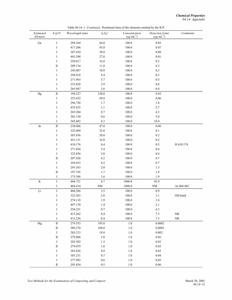
Chemical Properties04.14 Appendix
Table 04.14–1 Continued. Prominent lines of the elements emitted by the ICP.
EstimatedElement
S of I† Wavelength (nm) In/Ib‡ Concentration(µg mL-1)
Detection Limit(µg mL-1)
Comments
Test Methods for the Examination of Composting and Compost March 20, 200104.14–31
Ga I 294.364 64.0 100.0 0.05I 417.206 45.0 100.0 0.07I 287.424 38.0 100.0 0.08I 403.298 27.0 100.0 0.01I 250.017 16.0 100.0 0.2II 209.134 11.0 100.0 0.3I 245.007 10.0 100.0 0.3I 294.418 9.4 100.0 0.3I 271.965 5.7 100.0 0.5I 233.828 3.9 100.0 0.8I 265.987 3.6 100.0 0.8
Hg II 194.227 120.0 100.0 0.03I 253.652 49.0 100.0 0.06I 296.728 1.7 100.0 1.8I 435.835 1.1 100.0 2.7I 265.204 0.7 100.0 4.3I 302.150 0.6 100.0 5.0I 365.483 0.3 100.0 10.0
In II 230.606 47.0 100.0 0.06I 325.609 25.0 100.0 0.1I 303.936 20.0 100.0 0.2I 451.131 16.0 100.0 0.2I 410.176 6.4 100.0 0.5 H 410.174I 271.026 5.4 100.0 0.6I 325.856 5.0 100.0 0.6II 207.926 4.2 100.0 0.7I 256.015 4.2 100.0 0.7I 293.263 2.0 100.0 1.5II 197.745 1.7 100.0 1.8I 175.388 1.6 100.0 1.9
K I 404.721 0.7 1000.0 42.9I 404.414 NM 1000.0 NM Ar 404.442
Li I 460.286 3.5 100.0 0.9I 323.263 2.8 100.0 1.1 OH bandI 274.118 1.9 100.0 1.6I 497.170 1.4 100.0 2.1I 256.231 0.7 100.0 4.3I 413.262 0.4 100.0 7.5 NRI 413.256 0.4 100.0 7.5 NR
Mg II 279.553 195.0 1.0 0.0002II 280.270 100.0 1.0 0.0003I 285.213 19.0 1.0 0.002II 279.806 2.0 1.0 0.02I 202.582 1.3 1.0 0.02II 279.079 1.0 1.0 0.03I 383.826 0.9 1.0 0.03I 383.231 0.7 1.0 0.04I 277.983 0.6 1.0 0.05II 293.654 0.5 1.0 0.06
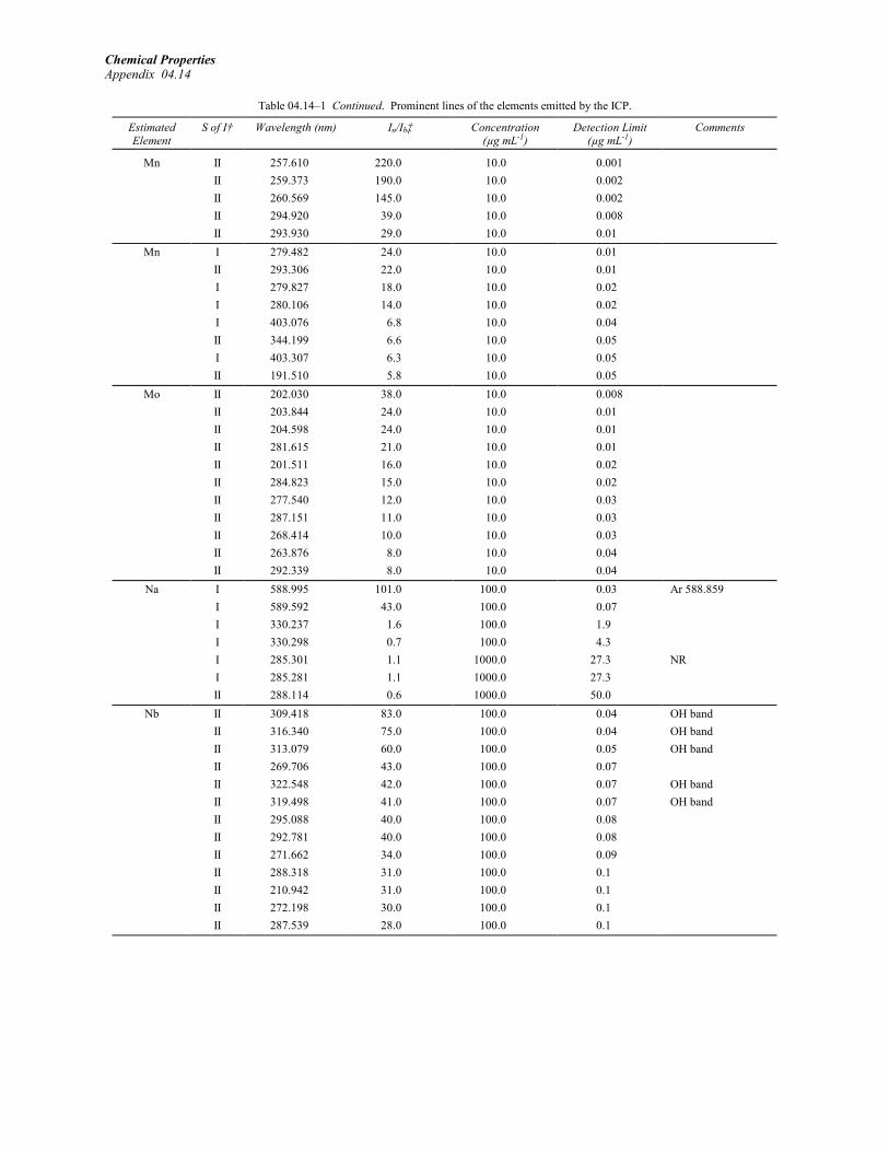
Chemical PropertiesAppendix 04.14
Table 04.14–1 Continued. Prominent lines of the elements emitted by the ICP.
EstimatedElement
S of I† Wavelength (nm) In/Ib‡ Concentration(µg mL-1)
Detection Limit(µg mL-1)
Comments
Mn II 257.610 220.0 10.0 0.001II 259.373 190.0 10.0 0.002II 260.569 145.0 10.0 0.002II 294.920 39.0 10.0 0.008II 293.930 29.0 10.0 0.01
Mn I 279.482 24.0 10.0 0.01II 293.306 22.0 10.0 0.01I 279.827 18.0 10.0 0.02I 280.106 14.0 10.0 0.02I 403.076 6.8 10.0 0.04II 344.199 6.6 10.0 0.05I 403.307 6.3 10.0 0.05II 191.510 5.8 10.0 0.05
Mo II 202.030 38.0 10.0 0.008II 203.844 24.0 10.0 0.01II 204.598 24.0 10.0 0.01II 281.615 21.0 10.0 0.01II 201.511 16.0 10.0 0.02II 284.823 15.0 10.0 0.02II 277.540 12.0 10.0 0.03II 287.151 11.0 10.0 0.03II 268.414 10.0 10.0 0.03II 263.876 8.0 10.0 0.04II 292.339 8.0 10.0 0.04
Na I 588.995 101.0 100.0 0.03 Ar 588.859I 589.592 43.0 100.0 0.07I 330.237 1.6 100.0 1.9I 330.298 0.7 100.0 4.3I 285.301 1.1 1000.0 27.3 NRI 285.281 1.1 1000.0 27.3II 288.114 0.6 1000.0 50.0
Nb II 309.418 83.0 100.0 0.04 OH bandII 316.340 75.0 100.0 0.04 OH bandII 313.079 60.0 100.0 0.05 OH bandII 269.706 43.0 100.0 0.07II 322.548 42.0 100.0 0.07 OH bandII 319.498 41.0 100.0 0.07 OH bandII 295.088 40.0 100.0 0.08II 292.781 40.0 100.0 0.08II 271.662 34.0 100.0 0.09II 288.318 31.0 100.0 0.1II 210.942 31.0 100.0 0.1II 272.198 30.0 100.0 0.1II 287.539 28.0 100.0 0.1
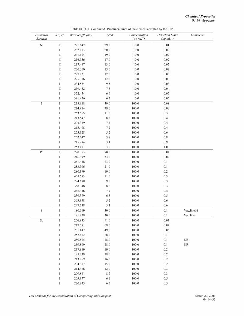
Chemical Properties04.14 Appendix
Table 04.14–1 Continued. Prominent lines of the elements emitted by the ICP.
EstimatedElement
S of I† Wavelength (nm) In/Ib‡ Concentration(µg mL-1)
Detection Limit(µg mL-1)
Comments
Test Methods for the Examination of Composting and Compost March 20, 200104.14–33
Ni II 221.647 29.0 10.0 0.01I 232.003 20.0 10.0 0.02II 231.604 19.0 10.0 0.02II 216.556 17.0 10.0 0.02II 217.467 13.0 10.0 0.02II 230.300 13.0 10.0 0.02II 227.021 12.0 10.0 0.03II 225.386 12.0 10.0 0.03I 234.554 9.5 10.0 0.03II 239.452 7.8 10.0 0.04I 352.454 6.6 10.0 0.05I 341.476 6.2 10.0 0.05
P I 213.618 39.0 100.0 0.08I 214.914 39.0 100.0 0.08I 253.565 11.0 100.0 0.3I 213.547 8.5 100.0 0.4I 203.349 7.4 100.0 0.4I 215.408 7.2 100.0 0.4I 255.328 5.2 100.0 0.6I 202.347 3.8 100.0 0.8I 215.294 3.4 100.0 0.9I 253.401 3.0 100.0 1.0
Pb II 220.353 70.0 100.0 0.04I 216.999 33.0 100.0 0.09I 261.418 23.0 100.0 0.1I 283.306 21.0 100.0 0.1I 280.199 19.0 100.0 0.2I 405.783 11.0 100.0 0.3I 224.688 9.0 100.0 0.3I 368.348 8.6 100.0 0.3I 266.316 7.7 100.0 0.4I 239.379 6.3 100.0 0.5I 363.958 5.2 100.0 0.6I 247.638 5.1 100.0 0.6
S I 180.669 30.0 100.0 0.1 Vac.line§§I 181.979 30.0 100.0 0.1 Vac line
Sb I 206.833 91.0 100.0 0.03I 217.581 68.0 100.0 0.04I 231.147 49.0 100.0 0.06I 252.852 28.0 100.0 0.1I 259.805 28.0 100.0 0.1 NRI 259.809 28.0 100.0 0.1 NRI 217.919 19.0 100.0 0.2I 195.039 18.0 100.0 0.2I 213.969 16.0 100.0 0.2I 204.957 15.0 100.0 0.2I 214.486 12.0 100.0 0.3I 209.841 8.7 100.0 0.3I 203.977 6.6 100.0 0.5I 220.845 6.5 100.0 0.5

Chemical PropertiesAppendix 04.14
Table 04.14–1 Continued. Prominent lines of the elements emitted by the ICP.
EstimatedElement
S of I† Wavelength (nm) In/Ib‡ Concentration(µg mL-1)
Detection Limit(µg mL-1)
Comments
I 287.792 4.7 100.0 0.6Se I 196.026 40.0 100.0 0.08
I 203.985 26.0 100.0 0.1I 206.279 10.0 100.0 0.3I 207.479 1.9 100.0 1.6I 199.511 0.6 100.0 5.0
Si I 251.611 250.0 100.0 0.01I 212.412 180.0 100.0 0.02I 288.158 110.0 100.0 0.03I 250.690 100.0 100.0 0.03I 252.851 95.0 100.0 0.03I 251.432 79.0 100.0 0.04I 252.411 75.0 100.0 0.04I 221.667 72.0 100.0 0.04I 251.920 61.0 100.0 0.05I 198.899 50.0 100.0 0.06I 221.089 47.0 100.0 0.06I 243.515 36.0 100.0 0.08I 190.134 23.0 100.0 0.1I 220.798 23.0 100.0 0.1I 205.813 23.0 100.0 0.1
Sn II 189.989 120.0 100.0 0.03I 235.484 31.0 100.0 0.1I 242.949 31.0 100.0 0.1I 283.999 27.0 100.0 0.1I 226.891 25.0 100.0 0.1I 224.605 25.0 100.0 0.1I 242.170 19.0 100.0 0.2I 270.651 18.0 100.0 0.2I 220.965 16.0 100.0 0.2I 286.333 14.0 100.0 0.2I 317.505 14.0 100.0 0.2 OH band
Sr II 407.771 72.0 1.0 0.0004II 421.552 39.0 1.0 0.0008II 216.596 36.0 10.0 0.008II 215.284 29.0 10.0 0.01II 346.446 13.0 10.0 0.02II 338.071 8.8 10.0 0.03II 430.545 4.8 10.0 0.06I 460.733 4.4 10.0 0.07II 232.235 2.9 10.0 0.1II 416.180 2.4 10.0 0.1
Te I 214.281 73.0 100.0 0.04I 225.902 17.0 100.0 0.2I 238.578 17.0 100.0 0.2I 214.725 14.0 100.0 0.2I 200.202 12.0 100.0 0.3I 238.326 11.0 100.0 0.3I 208.116 11.0 100.0 0.3I 199.418 6.3 100.0 0.5

Chemical Properties04.14 Appendix
Table 04.14–1 Continued. Prominent lines of the elements emitted by the ICP.
EstimatedElement
S of I† Wavelength (nm) In/Ib‡ Concentration(µg mL-1)
Detection Limit(µg mL-1)
Comments
Test Methods for the Examination of Composting and Compost March 20, 200104.14–35
I 225.548 2.7 100.0 1.1I 226.555 2.6 100.0 1.2
Ti II 334.941 79.0 10.0 0.0004II 336.121 57.0 10.0 0.0005II 323.452 56.0 10.0 0.005 OH bandII 337.280 45.0 10.0 0.007II 334.904 40.0 10.0 0.008II 308.802 39.0 10.0 0.008 OH bandII 307.864 37.0 10.0 0.008 OH bandII 338.376 37.0 10.0 0.008II 323.657 30.0 10.0 0.01 OH bandII 323.904 29.0 10.0 0.01 OH bandII 368.520 26.0 10.0 0.01
Tl II 190.864 74.0 100.0 0.04I 276.787 25.0 100.0 0.1I 351.924 15.0 100.0 0.2I 377.572 13.0 100.0 0.2I 237.969 7.0 100.0 0.4I 291.832 2.9 100.0 1.0I 223.785 2.2 100.0 1.4I 352.943 1.7 100.0 1.8I 258.014 1.7 100.0 1.8
V II 309.311 60.0 10.0 0.005 OH bandII 310.230 47.0 10.0 0.006 OH bandII 292.402 40.0 10.0 0.008II 290.882 34.0 10.0 0.009II 311.071 30.0 10.0 0.01 OH bandII 289.332 29.0 10.0 0.01II 268.796 29.0 10.0 0.01II 311.838 25.0 10.0 0.01 OH bandII 214.009 20.0 10.0 0.02II 312.528 20.0 10.0 0.02 OH bandII 327.612 19.0 10.0 0.02II 292.464 18.0 10.0 0.02II 270.094 17.0 10.0 0.02
Zn I 213.856 170.0 10.0 0.002II 202.548 75.0 10.0 0.004II 206.200 51.0 10.0 0.006I 334.502 2.2 10.0 0.1I 330.259 1.3 10.0 0.2I 481.053 1.3 10.0 0.2I 472.216 0.7 10.0 0.4I 328.233 0.6 10.0 0.5I 334.557 0.4 10.0 0.8I 280.106 0.4 10.0 0.8 NRI 280.087 0.4 10.0 0.8 NR

Chemical PropertiesAppendix 04.14
Table 04.14–1 Continued. Prominent lines of the elements emitted by the ICP.
EstimatedElement
S of I† Wavelength (nm) In/Ib‡ Concentration(µg mL-1)
Detection Limit(µg mL-1)
Comments
Zr II 343.823 42.0 10.0 0.007II 339.198 39.0 10.0 0.008II 257.139 31.0 10.0 0.01II 349.621 30.0 10.0 0.01II 357.247 30.0 10.0 0.01II 327.305 25.0 10.0 0.01II 256.887 22.0 10.0 0.01II 327.926 21.0 10.0 0.02II 267.863 20.0 10.0 0.02II 272.261 16.0 10.0 0.02II 273.486 14.0 10.0 0.02II 274.256 14.0 10.0 0.02II 270.013 12.0 10.0 0.03II 350.567 12.0 10.0 0.03II 355.660 12.0 10.0 0.03II 348.115 12.0 10.0 0.03II 256.764 11.0 10.0 0.03
Zr II 272.649 11.0 10.0 0.03II 330.628 11.0 10.0 0.03II 316.597 11.0 10.0 0.03 OH bandII 318.286 11.0 10.0 0.03 OH bandII 328.471 10.0 10.0 0.03II 274.586 10.0 10.0 0.03II 275.221 10.0 10.0 0.03II 357.685 10.0 10.0 0.03
† S of I = State of ionization. Symbols I, II, and III indicate that the spectral lines originate from the neutral atom, singly ionized, and doubly ionized states,respectively.
‡ In/Ib = Ratio of net analyte intensity to background intensity." Conc. = Concentration of the single element analyte solution used for the wavelength scans from which the prominent lines were determined.
Detection limits estimated from the In/Ib ratios using the formula: DL = 0.03C/(In/Ib) where C is concentration of analyte.# Includes interference information when a component of the background spectrum overlaps an analyte line (e.g., the Ba 389.178-nm line is located on the H
388.905-nm line) or when an analyte line is located in complex molecular band system (e.g., the OH 306.3-nm system) where band components may causespectral interferences. The notation of molecular bands does not preclude the use of analyte wavelengths within the band region.
†† NR = Not resolved. This description indicates components of an unresolved pair of lines.‡‡ Group NR indicates components of an unresolved group (three or more lines). Only the wavelength of the strongest line is listed.§§ Vacuum lines for S require either a vacuum or an Ar purged spectrometer, see " Selection of Wavelength."
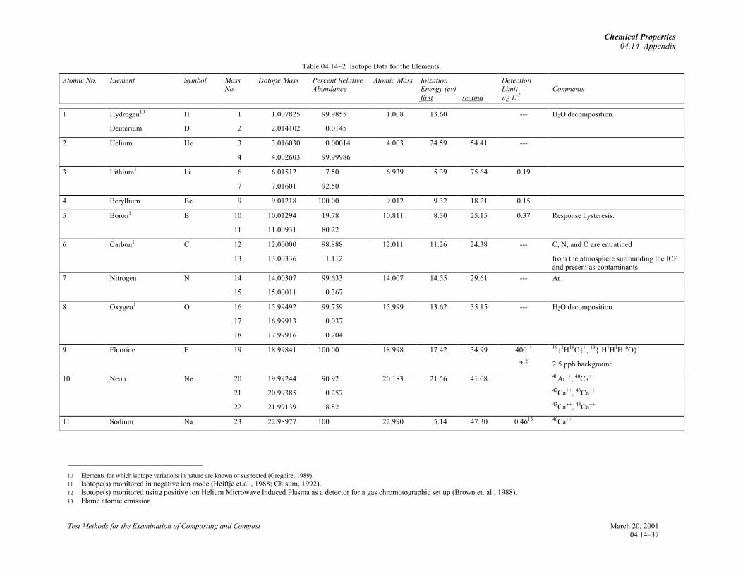
Chemical Properties04.14 Appendix
Table 04.14–2 Isotope Data for the Elements.
Atomic No. Element Symbol MassNo.
Isotope Mass Percent RelativeAbundance
Atomic Mass IoizationEnergy (ev)first second
DetectionLimitµg L-1
Comments
Test Methods for the Examination of Composting and Compost March 20, 200104.14–37
1 Hydrogen10 H 1 1.007825 99.9855 1.008 13.60 --- H2O decomposition.
Deuterium D 2 2.014102 0.0145
2 Helium He 3 3.016030 0.00014 4.003 24.59 54.41 ---
4 4.002603 99.99986
3 Lithium1 Li 6 6.01512 7.50 6.939 5.39 75.64 0.19
7 7.01601 92.50
4 Beryllium Be 9 9.01218 100.00 9.012 9.32 18.21 0.15
5 Boron1 B 10 10.01294 19.78 10.811 8.30 25.15 0.37 Response hysteresis.
11 11.00931 80.22
6 Carbon1 C 12 12.00000 98.888 12.011 11.26 24.38 --- C, N, and O are entratined
13 13.00336 1.112 from the atmosphere surrounding the ICPand present as contaminants
7 Nitrogen1 N 14 14.00307 99.633 14.007 14.55 29.61 --- Ar.
15 15.00011 0.367
8 Oxygen1 O 16 15.99492 99.759 15.999 13.62 35.15 --- H2O decomposition.
17 16.99913 0.037
18 17.99916 0.204
9 Fluorine F 19 18.99841 100.00 18.998 17.42 34.99 40011 19{1H18O}+, 19{1H1H1H16O}+
?12 2.5 ppb background
10 Neon Ne 20 19.99244 90.92 20.183 21.56 41.08 40Ar++, 40Ca++
21 20.99385 0.257 42Ca++, 43Ca++
22 21.99139 8.82 43Ca++, 44Ca++
11 Sodium Na 23 22.98977 100 22.990 5.14 47.30 0.4613 46Ca++
10 Elements for which isotope variations in nature are known or suspected (Gregoire, 1989).11 Isotope(s) monitored in negative ion mode (Heiftje et.al., 1988; Chisum, 1992).12 Isotope(s) monitored using positive ion Helium Microwave Induced Plasma as a detector for a gas chromotographic set up (Brown et. al., 1988).13 Flame atomic emission.

Chemical PropertiesAppendix 04.14
Table 04.14–2 Isotope Data for the Elements.
Atomic No. Element Symbol MassNo.
Isotope Mass Percent RelativeAbundance
Atomic Mass IoizationEnergy (ev)first second
DetectionLimitµg L-1
Comments
March 20, 2001 Test Methods for the Examination of Composting and Compost04.14–38
12 Magnesium1 Mg 24 23.98504 78.70 24.312 7.65 15.03 0.35 48Ca++, 24{12C12C}+
25 24.98584 10.13
25.98259
13 Aluminum Al 27 26.98154 100.00 26.982 5.99 18.83 0.21 27{12C1H14N}+
14 Silicon Si 28 27.97693 92.21 28.086 8.15 16.34 1314 28{12C16O}+
29 28.97650 4.70 29{12C1H16O}+
30 29.97377 3.09 30{16O14N}+
15 Phosphorous P 31 30.97376 100.00 30.974 10.48 19.72 785 31{1H16O14N}+
16 Sulfur1 S 32 31.97207 95.018 32.064 10.36 23.4 5002 32{16O16O}+
33 32.97146 0.760 33{1H16O16O}+
34 33.96787 4.215 34{1H16O1H16O}+
36 35.96708 0.014 36Ar+
17 Chlorine1 Cl 35 34.96885 75.53 35.453 13.02 23.80 32
37 36.96590 24.47 0.083 in units of pg/sec3
18 Argon1 Ar 36 35.96755 0.337 39.948 15.76 27.63
38 37.96273 0.063
40 39.96238 99.600 --- 40K+, 40Ca+, 40{24Mg16O}+
19 Potassium1 K 39 38.96371 93.10 39.102 4.34 31.82 0.424 39{1H38Ar}+
40 39.974 0.0118 40Ar+, 40Ca+, 40{24Mg16O}+
K 41 40.96183 6.88 41{1H40Ar}+, 41{25Mg16O}+, Holden,1972.
20 Calcium Ca 40 39.96259 96.97 40.08 6.11 11.87 0.285 40Ar+, 40K+, 40{24Mg16O}+
42 41.95863 0.64 42{12C16O14N}+, 84Sr++, 42{26Mg16O}+
43 42.95878 0.145 43{12C1H16O14N}+, 86,87Sr++
44 43.95549 2.06 44{12C16O16O}+, 87,88Sr++
46 45.95369 0.003 46Ti+, 46{16O16O14N}+
14 ICP atomic emission with ultrasonic nebulization.

Chemical Properties04.14 Appendix
Table 04.14–2 Isotope Data for the Elements.
Atomic No. Element Symbol MassNo.
Isotope Mass Percent RelativeAbundance
Atomic Mass IoizationEnergy (ev)first second
DetectionLimitµg L-1
Comments
Test Methods for the Examination of Composting and Compost March 20, 200104.14–39
48 47.95253 0.185 48Ti+, 48{16O16O16O}+
21 Scandium Sc 45 44.956 100.00 44.956 6.56 12.80 0.15 45{12C1H16O16O}+
22 Titanium Ti 46 45.95263 7.93 47.90 6.84 13.64 46{16O16O14N}+
47 46.95177 7.28 47{1H16O16O14N}+, 47{31P16O}+
48 47.94795 73.94 0.49 48Ca+, 48{16O16O16O}+, 48{31P1H16O}+
49 48.94787 5.51 49{35Cl14N}+
50 49.94478 5.34 50{14N36Ar}+, 50V+, 50Cr+
23 Vanadium V 50 49.94716 0.24 50.942 6.74 14.65 50{14N36Ar}+, 50Ti+, 50Cr+
51 50.9440 99.76 0.25 51{37Cl14N}+, 51{35Cl16O}+
24 Chromium Cr 50 49.9460 4.31 51.996 6.77 16.49 50{14N36Ar}+, 50V+, 50Ti+
52 51.9405 83.76 0.21 52{12C40Ar}+, 52{16O36Ar}+,52{35Cl1H16O}+
53 52.9407 9.55 53{12C1H40Ar}+, 53{1H16036Ar}+,53{37Cl16O}+
54 53.9389 2.38 54Fe+,54{16O38Ar}+, 54{14N40Ar}+,54{37Cl1H16O}+
25 Manganese Mn 55 54.9381 100.00 54.938 7.43 15.64 0.26 55{1H16038Ar}+
26 Iron Fe 54 53.9396 5.82 55.847 7.90 16.18 54Cr+, 54{16O38Ar}+, 54{14N40Ar}+,54{37Cl1H16O}+
56 55.9349 91.66 0.4815 56{16O40Ar}+, 56{40Ca16O}+
57 56.9354 2.19 57{1H16O40Ar}+
58 57.9333 0.33 58Ni+, 58{42Ca16O}+
27 Cobalt Co 59 58.9332 100.00 58.933 7.87 17.05 0.23 59{43Ca16O}+, 59{42Ca1H16O}+
28 Nickel Ni 58 57.9353 67.88 58.71 7.63 18.15 0.49 58Fe+, 58{42Ca16O}+
60 59.9308 26.23 60{44Ca16O}+, 60{24Mg36Ar}+
61 60.9311 1.19 61{44Ca1H16O}+
62 61.9283 3.66 62{46Ca16O}+, 62{26Mg36Ar}+
64 63.9280 1.08 64Zn+, 64{48Ca16O}+, 64{24Mg40Ar}+,64{31P1H16O16O}+
15 Graphite furnace atomic absorption.

Chemical PropertiesAppendix 04.14
Table 04.14–2 Isotope Data for the Elements.
Atomic No. Element Symbol MassNo.
Isotope Mass Percent RelativeAbundance
Atomic Mass IoizationEnergy (ev)first second
DetectionLimitµg L-1
Comments
March 20, 2001 Test Methods for the Examination of Composting and Compost04.14–40
29 Copper Cu 63 62.9296 69.09 63.54 7.73 20.29 0.34 63{23Na40Ar}+, 63{31P16O16O}+
65 64.9278 30.91 65{25Mg40Ar}+, 130Ba++
30 Zinc Zn 64 63.9291 48.89 65.37 9.39 17.96 0.78 64Ni+, 64{24Mg40Ar}+, 64{48Ca16O}+,64{31P1H16O16O}+, 64{32S16O16O}+,64{32S32S}+, 64{63Cu1H}+
66 65.9260 27.81 66{26Mg40Ar}+, 66{31P35Cl}+,66{34S16O16O}+, 66{65Cu1H}+, 132Ba++
67 66.9271 4.11 67{35Cl16O16O}+, 67{1H34S16O16O}+,134,135Ba++
68 67.9248 18.57 68{32S36Ar}+, 68{31P37Cl}+,68{35Cl1H16O16O}+,
70 69.9253 0.62 70Ge+, 139La++, 70{37Cl1H16O16O}+,140Ce++, 141Pr++
31 Gallium Ga 69 68.9256 60.4 69.72 6.00 20.51 0.34 69{37Cl16O16O}+, 137,138Ba++, 138,139La++,138Ce++
71 70.9247 39.6 142Ce++, 141Pr++, 142,143Nd++
32 Germanium Ge 70 69.9243 20.52 72.59 7.89 15.93 0.44 70Zn+, 139La++, 70{37Cl1H16O16O}+,140Ce++, 70{35Cl2}+, 141Pr++
72 71.9221 27.43 72{16O56Fe}+, 143,144,145Nd++, 144Sm++,72{35Cl37Cl}+
73 72.9235 7.76 73{16O57Fe}+, 73{1H16O56Fe}+, 145,146Nd++,147Sm++
74 73.9212 36.54 74Se+, 148Nd++, 147,148,149Sm++, 74{37Cl2}+
76 75.9214 7.76 76Se+, 76{36Ar40Ar}+, 152Sm++, 151,153Eu++,152Gd++
33 Arsenic As 75 74.9216 100.00 74.922 9.82 18.63 0.55 75{35Cl40Ar}+, 150Nd++, 149,150Sm++,151Eu++
34 Selenium1 Se 74 73.9225 0.87 78.96 9.75 21.5 74Ge+, 148Nd++, 147,148,149Sm++
76 75.9192 9.02 76Ge+, 76{36Ar40Ar}+, 152Sm++, 151,153Eu++,152Gd++
77 76.9199 7.58 2.1 77{37Cl40Ar}+, 154Sm++, 153Eu++,154,155Gd++
78 77.9173 23.52 78Kr+, 78{38Ar40Ar}+, 155,156,157Gd++,156Dy++
80 79.9165 49.82 80Kr+, 80{40Ar40Ar}+, 80{40Ca40Ar}+,160Gd++, 160,161Dy++
82 81.9167 9.19 82Kr+, 82{42Ca40Ar}+, 163,164Dy++, 165Ho++,164Er++

Chemical Properties04.14 Appendix
Table 04.14–2 Isotope Data for the Elements.
Atomic No. Element Symbol MassNo.
Isotope Mass Percent RelativeAbundance
Atomic Mass IoizationEnergy (ev)first second
DetectionLimitµg L-1
Comments
Test Methods for the Examination of Composting and Compost March 20, 200104.14–41
35 Bromine1 Br 79 78.9183 50.537 79.909 11.85 21.6 11 79{1H38Ar40Ar}+, 157,158Gd++, 159Tb++,158Dy++
81 80.9163 49.463 81{1H40Ar40Ar}+, 81{32S1H16O16O16O}+,161,162,163Dy++, 162Er++, Responsehysteresis.
36 Krypton Kr 78 77.9204 0.35 83.80 14.00 24.57 78Se+, 78{38Ar40Ar}+, 155,156,157Gd++,156Dy++
80 79.9164 2.27 80Se+, 80{40Ar40Ar}+, 160Gd++, 160,161Dy++
82 81.9135 11.56 82Se+, 82{42Ca40Ar}+, 163,164Sm++, 165Ho++,164Er++
83 82.9141 11.55 83{43Ca40Ar}+, 165Ho++, 166,167Er++
84 83.9115 56.90 84Sr+, 84{44Ca40Ar}+, 167,168Er++, 169Tm++,168Yb++
86 85.9106 17.37 86Sr+, 86{46Ca40Ar}+, 171,172,173Yb++
37 Rubidium Rb 85 84.9118 72.15 85.47 4.18 27.5 0.13 170Er++, 169Tm++, 170,171Yb++
87 86.9161 27.85 87Sr+, 173,174Yb++
38 Strontium1 Sr 84 83.9134 0.56 87.62 5.69 11.03 84Kr+, 167,168Er++, 169Tm++, 168Yb++
86 85.9093 9.86 86Kr+, 171,172,173Yb++
87 86.9089 7.02 87Rb+, 173,174Yb++
88 87.9056 82.56 0.20 176Yb++
39 Yttrium Y 89 88.9059 100.00 88.905 6.53 12.23 0.15
40 Zirconium Zr 90 89.9047 51.46 91.22 6.95 13.13 0.26
91 90.9056 11.23
92 91.9050 17.11 92Mo+
94 93.9063 17.40 94Mo+
96 95.9083 2.80 96Mo+, 96Ru+
41 Niobium Nb 93 92.9064 100.00 92.906 6.88 14.0 0.14

Chemical PropertiesAppendix 04.14
Table 04.14–2 Isotope Data for the Elements.
Atomic No. Element Symbol MassNo.
Isotope Mass Percent RelativeAbundance
Atomic Mass IoizationEnergy (ev)first second
DetectionLimitµg L-1
Comments
March 20, 2001 Test Methods for the Examination of Composting and Compost04.14–42
42 Molybdenum Mo 92 91.9068 15.84 95.94 7.10 16.15 92Zr+
94 93.9051 9.04 94Zr+
95 94.9058 15.72
96 95.9047 16.53 96Zr+, 96Ru+
97 96.9060 9.46
98 97.9054 23.78 0.27 98Ru+
100 99.9075 9.63 100Ru+
43 Technetium Tc 97 96.9 7.28 15.26 t½ = 2.6E6 years16, 17
99 98.9 t½ = 213,000 years8
44 Ruthenium Ru 96 95.9076 5.51 101.07 7.36 16.76 96Zr+, 96Mo+
98 97.9053 1.87 98Mo+
99 98.9059 12.72
100 99.9042 12.62 100Mo+, 100{84Sr16O}+
101 100.9056 17.07
102 101.9043 31.63 0.20 102Pd+, 102{86Sr16O}+
104 103.9054 18.58 104Pd+, 104{88Sr16O}+
45 Rhodium Rh 103 102.9055 100.00 102.905 7.45 18.07 ---18 103{87Sr16O}+
46 Palladium Pd 102 101.9056 0.96 106.4 8.33 19.42 102{86Sr16O}+
104 103.9040 10.97 104Ru+, 104{88Sr16O}+
105 104.9051 22.23 105{89Y16O}+
106 105.9035 27.33 0.49 106Cd+, 106{90Zr16O}+, 106{89Y1H16O}+
Pd 108 107.9039 26.71 108Cd+, 108{92Zr16O}+, 108{92Mo16O}+
110 109.9052 11.81 110Cd+, 110{94Zr16O}+, 110{94Mo16O}+
16 Isotope of element having longest half-life (Weast and Astle, 1979; Holden and Walker, 1972.)17 Most commonly available long-lived isotope of element (Weast and Astle, 1979).18 Isotope used as internal standard in author's lab. Thus, the detection limit has not, as yet, been determined.

Chemical Properties04.14 Appendix
Table 04.14–2 Isotope Data for the Elements.
Atomic No. Element Symbol MassNo.
Isotope Mass Percent RelativeAbundance
Atomic Mass IoizationEnergy (ev)first second
DetectionLimitµg L-1
Comments
Test Methods for the Examination of Composting and Compost March 20, 200104.14–43
47 Silver1 Ag 107 106.9051 51.817 107.87 7.58 21.48 0.37 107{91Zr16O}+
109 108.9048 48.183 109{93Nb16O}+
48 Cadmium Cd 106 105.9065 1.22 112.40 8.99 16.90 106Pd+, 106{90Zr16O}+, 106{89Y1H16O}+
108 107.9042 0.88 108Pd+, 108{92Zr16O}+, 108{92Mo16O}+
110 109.9030 12.39 110Pd+, 110{94Zr16O}+, 110{94Mo16O}+
111 110.9042 12.75 0.39
112 111.9028 24.07 112Sn+, 112{96Zr16O}+, 112{96Mo16O}+
113 112.9044 12.26 113In+, 113{97Mo16O}+
114 113.9034 28.86 114Sn+, 114{98Mo16O}+
116 115.9048 7.58 116Sn+, 116{100Mo16O}+, 232Th++
49 Indium In 113 112.9041 4.28 114.82 5.79 18.86 113Cd+, 113{97Mo16O}+
115 114.9039 95.72 0.10 115Sn+
50 Tin Sn 112 111.9048 0.96 118.69 7.34 14.63 112Cd+, 112{96Zr16O}+, 112{96Mo16O}+
114 113.9028 0.66 114Cd+, 114{98Mo16O}+
115 114.9034 0.35 115In+
116 115.9017 14.30 116Cd+, 116{100Mo16O}+, 232Th++
117 116.9030 7.61
118 117.9016 24.03
119 118.9033 8.58
120 119.9022 32.85 0.20 120Te+
122 121.9035 4.72 122Te+
124 123.9053 5.94 124Te+, 124Xe+
51 Antimony Sb 121 120.904 57.25 121.75 7.85 16.5 0.20
123 122.9042 42.75 123Te+

Chemical PropertiesAppendix 04.14
Table 04.14–2 Isotope Data for the Elements.
Atomic No. Element Symbol MassNo.
Isotope Mass Percent RelativeAbundance
Atomic Mass IoizationEnergy (ev)first second
DetectionLimitµg L-1
Comments
March 20, 2001 Test Methods for the Examination of Composting and Compost04.14–44
52 Tellurium Te 120 119.9040 0.089 127.60 9.01 18.6 120Sn+
122 121.9031 2.46 122Sn+
123 122.9043 0.87 123Sb+
124 123.9028 4.61 124Sn+, 124Xe+
125 124.9044 6.99
126 125.9033 18.71 0.33 126Xe+
Te 128 127.9045 31.79 128Xe+, 128{112Sn16O}+
130 129.9062 34.48 130Ba+, 130Xe+, 130{114Sn16O}+
53 Iodine I 127 126.9045 100.00 126.904 10.46 19.09 5.1 Response hysteresis.
54 Xenon Xe 124 123.9061 0.096 131.30 12.13 21.21 124Sn+, 124Te+
126 125.9043 0.090 126Te+
128 127.9035 1.919 128Te+, 128{112Sn16O}+
129 128.9048 26.44 129{89Y40Ar}+
130 129.9035 4.08 130Ba+, 130Te+, 130{114Sn16O}+
131 130.9051 21.18 131{115Sn16O}+
132 131.9042 26.89 132Ba+, 132{116Sn16O}+
134 133.9054 10.44 134Ba+, 134{118Sn16O}+
136 135.9072 8.87 136Ba+, 136{120Sn16O}+
55 Cesium Cs 133 132.9054 100.00 132.905 3.89 25.08 0.17 133{117Sn16O}+
56 Barium Ba 130 129.9063 0.101 137.34 5.21 10.00 130Xe+, 130Te+, 130{114Sn16O}+
132 131.9051 0.097 132Xe+, 132{116Sn16O}+
134 133.9045 2.42 134Xe+, 134{118Sn16O}+
135 134.9057 6.59 135{119Sn16O}+
Ba 136 135.9046 7.81 136Xe+, 136Ce+, 136{120Sn16O}+
137 136.9058 11.32
138 137.9052 71.66 0.18 138Ce+, 138La+

Chemical Properties04.14 Appendix
Table 04.14–2 Isotope Data for the Elements.
Atomic No. Element Symbol MassNo.
Isotope Mass Percent RelativeAbundance
Atomic Mass IoizationEnergy (ev)first second
DetectionLimitµg L-1
Comments
Test Methods for the Examination of Composting and Compost March 20, 200104.14–45
57 Lanthanum La 138 137.9072 0.089 138.91 5.61 11.06 138Ba+, 138Ce+
139 138.9064 99.911 0.23
58 Cerium Ce 136 135.9072 0.193 140.12 5.57 10.85 136Xe+, 136Ba+
138 137.9060 0.250 138Ba+, 138La+
140 139.9055 88.48 0.25 140{124Sn16O}+, 140{139La1H}+
142 141.9093 11.07 142Nd+
59 Praeseodymium Pr 141 140.9077 100.00 140.907 5.42 10.55 0.31
60 Neodymium1 Nd 142 141.9078 27.11 144.24 5.45 10.73 0.35 142Ce+
143 142.9099 12.17
144 143.9101 23.85 144Sm+
145 144.9126 8.30
146 145.9132 17.22 146{130Ba16O}+
148 147.9169 5.73 148Sm+, 148{132Ba16O}+
150 149.9209 5.62 150Sm+, 150{134Ba16O}+
61 Promethium Pm 145 144.9 t = 18 years4, 145Nd+
147 146.9 t = 2.623 years3, 147Sm+
62 Samarium1 Sm 144 143.9121 3.09 150.35 5.6319 11.07 144Nd+
147 146.9149 14.97
148 147.9149 11.24 148Nd+, 148{132Ba16O}+
149 148.9172 13.83 0.39
150 149.9173 7.44 150Nd+, 150{134Ba16O}+
152 151.9198 26.72 152Gd+, 152{136Ba16O}+
154 153.9222 22.71 154Gd+, 154{138Ba16O}+
19 A.L. Gray, personal communication regarding revised ionization potentials.

Chemical PropertiesAppendix 04.14
Table 04.14–2 Isotope Data for the Elements.
Atomic No. Element Symbol MassNo.
Isotope Mass Percent RelativeAbundance
Atomic Mass IoizationEnergy (ev)first second
DetectionLimitµg L-1
Comments
March 20, 2001 Test Methods for the Examination of Composting and Compost04.14–46
63 Europium Eu 151 150.9199 47.82 151.96 5.64 11.25 0.31 151{135Ba16O}+
153 152.9213 52.18 153{137Ba16O}+
64 Gadolinium Gd 152 151.9198 0.20 157.25 6.16 12.1 152Sm+, 152{136Ba16O}+
154 153.9209 2.15 154Sm+, 154{138Ba16O}+
155 154.9226 14.73 155{139La16O}+
156 155.9221 20.47 156Dy+, 156{140Ce16O}+
157 156.9240 15.68 157{141Pr16O}+
158 157.9241 24.87 0.22 158Dy+, 158{142Ce16O}+, 158{142Nd16O}+,158{79Br2}+
160 159.9271 21.90 160Dy+, 160{144Nd16O}+, 160{144Sm16O}+,160{79Br81Br}+
65 Terbium Tb 159 158.9254 100.00 158.925 5.98 11.52 0.26 159{143Nd16O}+
66 Dysprosium Dy 156 155.9243 0.052 162.50 5.93 11.67 156Gd+, 156{140Ce16O}+
158 157.9244 0.090 158Gd+, 158{142Ce16O}+, 158{142Nd16O}+,158{79Br2}+
160 159.9252 2.29 160Gd+, 160{144Nd16O}+, 160{144Sm16O}+,160{79Br81Br}+
161 160.9270 18.88 161{145Nd16O}+
162 161.9268 25.53 162Er+, 162{146Nd16O}+, 162{81Br2}+
163 162.9288 24.97 0.32 163{147Sm16O}+
164 163.9292 28.18 164Er+, 164{148Nd16O}+, 164{148Sm16O}+
67 Holmium Ho 165 164.9304 100.00 164.930 6.02 11.80 0.20 165{149Sm16O}+
68 Erbium Er 162 161.9283 0.136 167.26 6.10 11.93 162Dy+, 162{146Nd16O}+, 162{81Br2}+
164 163.9292 1.56 164Dy+, 164{148Nd16O}+, 164{148Sm16O}+
166 165.9303 33.41 166{150Nd16O}+, 166{150Sm16O}+
167 166.9321 22.94 0.43
Er 168 167.9324 27.07 168Yb+, 168{152Sm16O}+, 168{152Gd16O}+
170 169.9355 14.88 170Yb+, 170{154Sm16O}+, 170{154Gd16O}+
69 Thulium Tm 169 168.9343 100.00 168.934 6.18 12.05 0.27 169{153Eu16O}+

Chemical Properties04.14 Appendix
Table 04.14–2 Isotope Data for the Elements.
Atomic No. Element Symbol MassNo.
Isotope Mass Percent RelativeAbundance
Atomic Mass IoizationEnergy (ev)first second
DetectionLimitµg L-1
Comments
Test Methods for the Examination of Composting and Compost March 20, 200104.14–47
70 Ytterbium Yb 168 167.9339 0.135 173.04 6.22 12.17 168Er+, 168{152Sm16O}+, 168{152Gd16O}+
170 169.9348 3.03 170Er+, 170{154Sm16O}+, 170{154Gd16O}+
171 170.9364 14.31 171{155Gd16O}+
172 171.9364 21.82 172{156Gd16O}+, 172{156Dy16O}+
173 172.9382 16.13 173{157Gd16O}+
174 173.9389 31.84 0.42 174Hf+, 174{158Gd16O}+, 174{158Dy16O}+
176 175.9426 12.73 176Lu+, 176Hf+, 176{160Gd16O}+,176{160Dy16O}+
71 Lutetium Lu 175 174.9408 97.41 174.97 6.15 13.9 0.21 175{159Tb16O}+
176 175.9427 2.59 176Yb+, 176Hf+, 176{160Gd16O}+, 176
72 Hafnium Hf 174 173.9401 0.18 178.49 6.6510 14.9210 174Yb+, 174{158Gd16O}+, 174{158Dy16O}+
Hf 176 175.9414 5.20 176Yb+, 176{160Gd16O}+, 176{160Dy16O}+
177 176.9433 18.50 177{161Dy16O}+
178 177.9437 27.14 178{162Dy16O}+, 178{162Er16O}+
179 178.9458 13.75 179{163Dy16O}+
180 179.9466 35.24 0.50 180Ta+, 180W+, 180{164Dy16O}+,180{164Er16O}+
73 Tantalum Ta 180 179.9476 0.012 180.948 7.88 16.2 180Hf+, 180W+, 180{164Dy16O}+,180{164Er16O}+
181 180.9480 99.988 0.25 181{165Ho16O}+
74 Tungsten W 180 179.9467 0.14 183.85 7.98 17.7 180Hf+, 180Ta+, 180{164Dy16O}+,180{164Er16O}+
182 181.9483 26.41 182{166Er16O}+
183 182.9503 14.40 183{167Er16O}+
184 183.9510 30.64 ---20 184Os+, 184{168Er16O}+, 184{168Yb16O}+
186 185.9544 28.41 186Os+, 186{170Er16O}+, 186{170Yb16O}+
75 Rhenium Re 185 184.9530 37.07 186.2 7.87 16.6 185{169Tm16O}+
187 186.9558 62.93 0.15 187Os+, 187{171Yb16O}+
20 Tungsten in routinely present in our test solutions at 100 ìg/ml. Thus, there is a relatively high residual background that inordinately inflates the Method Detection Limit (MDL) determination.

Chemical PropertiesAppendix 04.14
Table 04.14–2 Isotope Data for the Elements.
Atomic No. Element Symbol MassNo.
Isotope Mass Percent RelativeAbundance
Atomic Mass IoizationEnergy (ev)first second
DetectionLimitµg L-1
Comments
March 20, 2001 Test Methods for the Examination of Composting and Compost04.14–48
76 Osmium1 Os 184 183.9526 0.02 190.2 8.73 17.0 184W+, 184{168Er16O}+, 184{168Yb16O}+
186 185.9539 1.59 186W+, 186{170Er16O}+, 186{170Yb16O}+
187 186.9558 1.64 187Re+, 187{171Yb16O}+
188 187.9559 13.3 188{172Yb16O}+
189 188.9582 16.1 189{173Yb16O}+
190 189.9585 26.4 190Pt+, 190{174Yb16O}+, 190{174Hf16O}+
192 191.9615 41.0 ---21 192Pt+, 192{176Yb16O}+, 192{176Hf16O}+,192{176Lu16O}+
77 Iridium Ir 191 190.9606 37.3 192.2 9.1210 191{175Lu16O}+
193 192.9626 62.7 0.75 193{177Hf16O}+
78 Platinum Pt 190 189.9600 0.013 195.09 8.96 18.56 190Os+, 190{174Yb16O}+, 190{174Hf16O}+
192 191.9611 0.78 192Os+, 192{176Yb16O}+, 192{176Hf16O}+,192{176Lu16O}+
194 193.9627 32.9 194{178Hf16O}+
195 194.9648 33.8 0.31 195{179Hf16O}+
Pt 196 195.9650 25.3 196Hg+, 196{180Hf16O}+, 196{180W16O}+,196{180Ta16O}+
198 197.9679 7.21 198Hg+, 198{182W16O}+
79 Gold Au 197 196.9666 100.00 196.967 9.23 20.5 0.28 197{181Ta16O}+
80 Mercury1 Hg 196 195.9658 0.146 200.59 10.44 18.75 196Pt+, 196{180Hf16O}+, 196{180W16O}+,196{180Ta16O}+
198 197.9668 10.02 198Pt+, 198{182W16O}+
199 198.9683 16.84 199{183W16O}+
200 199.9683 23.13 200{184W16O}+
201 200.9703 13.22 201{185Re16O}+
Hg 202 201.9706 29.80 ---22 202{186W16O}+, Response hysteresis.
204 203.9735 6.85
21 Isotopes of element not available for instrument calibration or MDL determinations.22 MDL not yet evaluated.

Chemical Properties04.14 Appendix
Table 04.14–2 Isotope Data for the Elements.
Atomic No. Element Symbol MassNo.
Isotope Mass Percent RelativeAbundance
Atomic Mass IoizationEnergy (ev)first second
DetectionLimitµg L-1
Comments
Test Methods for the Examination of Composting and Compost March 20, 200104.14–49
81 Thallium Tl 203 202.9724 29.5 204.37 6.11 20.42 203{187Re16O}+
205 204.9744 70.5 0.11
82 Lead1 Pb 204 203.9731 1.48 207.19 7.42 15.03 204Hg+
206 205.9745 23.6
207 206.9759 22.6
208 207.9767 52.3 0.33
83 Bismuth Bi 209 208.9804 100.0 208.98 7.29 16.68 0.15
84 Polonium Po 209 208.9824 8.43 ---12 t½ = 102 years7
85 Astatine At 210 209.9870 9.5 ---12 t½ = 8.1 hours7
86 Radon Rn 222 222.0176 10.746 ---12 t½ = 3.824 days7
87 Francium Fr 223 223.0198 4 ---12 t½ = 22 minutes7
88 Radium Ra 226 226.0254 5.28 10.144 ---12 t½ = 1600 years7,8
89 Actinium Ac 227 227.0278 6.9 12.1 ---12 t½ = 21.77 years7
90 Thorium Th 232 232.0381 100.00 232.04 6.0810 11.5 ---12 t½ = 1.4E10 years7
91 Protactinium Pa 231 231.0359 ---12 t½ = 32,500 years7
92 Uranium U 234 234.0410 0.0057 238.03 6.0510 14.7210 t½ = 247,000 years
235 235.0439 0.72 t½ = 7.1E8 years
238 238.0508 99.27 0.031 t½ = 4.51E9 years
93 Neptunium Np 237 237.0482 99+ ---12 t½ = 2.14E6 years7,8
94 Plutonium Pu 238 238.0496 5.1 t½ = 87.8 years‡, 238U+
239 239.0522 t½ = 2.439E4 years, 239{238U1H}+
240 240.0538 t½ = 6540 years
244 244.0642 244{238U16O}+, t½ = 8.3E7 years7

Chemical PropertiesAppendix 04.14
Table 04.14–2 Isotope Data for the Elements.
Atomic No. Element Symbol MassNo.
Isotope Mass Percent RelativeAbundance
Atomic Mass IoizationEnergy (ev)first second
DetectionLimitµg L-1
Comments
March 20, 2001 Test Methods for the Examination of Composting and Compost04.14–50
95 Americium Am 241 241.0568 t½ = 433 years
243 243.0614 ---12 t½ = 7,370 years7,8
96 Curium Cm 244 244.0628 t½ = 17.9 years
247 247.0704 ---12 t½ = 1.54E7 years7,8
ACKNOWLEDGEMENT—The authors of the ICP section and TMECC editors gratefully acknowledge permission to reproduce much of the isotope data from Dr. A.R. Gray, the surviving editor,and Blackie, the publisher (Date and Gray, 1989).

Chemical Properties04.14 Appendix
Test Methods for the Examination of Composting and Compost March 20, 200104.14–51
Table 04.14–3 Detection limits in an ideal solution (pure water), 10% HCl, and in a simulated arid soil digest.
Ideal Solution† 10% HCl‡Simulated Soil
Digest"Element µg mL-1 µg mL-1 µg mL-1
Ag 0.004Al 0.0002 0.03As 0.04 0.02 0.7Au 0.04B 0.0007 0.002 0.03Ba 0.00002 0.001 0.001Be 0.0004Bi 0.05Ca 0.00002 0.002Cd 0.002 0.001 0.006Ce 0.0007Co 0.003 0.01 0.02Cr 0.0003 0.003 0.01CsCu 0.0001 0.003 0.01Fe 0.0003 0.003Ga 0.0006Hf 0.01Hg 0.001 0.02 0.2In 0.03K 0.1La 0.00005Li 0.0003
Mg 0.00001 0.0004Mn 0.00006 0.001Mo 0.0002 0.004 0.02Na 0.0002 0.01Nb 0.00007Ni 0.0004 0.005 0.009P 0.02 0.03
Pb 0.002 0.03 0.07Pt 0.08Sb 0.2Se 0.02 0.2Si 0.01Sn 0.03Sr 0.00002 0.0006 0.007Ta 0.002Ti 0.00007 0.002U 0.03V 0.0002W 0.0007Zn 0.002 0.002 0.008Zr 0.0004
†Data from Robin (1979).‡ Data from Soltanpour et al. (1982)." Data from Soltanpour et al. (1982). Simulated soil digest contained 10% HCl and the following elements at the given concentrations in micrograms per milliliter:Al = 1,500; Fe = 500; K = 400; Ca = 200; Na = 200; Mg = 100; Ti = 60; Mn = 20; P = 15.

Chemical PropertiesAppendix 04.14
March 20, 2001 Test Methods for the Examination of Composting and Compost04.14–52
Table 04.14–4. Examples of some interelemental spectral interferences observed in an ICP spectrometer atthe Colorado State University Soil Testing Laboratory (Soltanpour, et al, 1982).
Wavelength, nm
324.7 206.2x2
213.6x2
202.0 214.4 228.6 267.7 407.7 249.7 455.4 220.3 253.6 193.6 196.0
Cu Zn Ni Mo Cd Co Cr Sr B Ba Pb Hg As Se
AffectingElement
Concen-tration (µg
mL-1)Apparent concentration of affected elements, µg mL-1
K 400† -- -- -- -- -- -- -- -- -- -- -- -- -- --Ca 50 -- -- -- -- -- -- -- 0.003 -- -- -- -- -- --
200† -- -- -- -- -- -- 0.002 0.015 -- -- -- 0.024 -- --500 -- -- -- -- -- -- 0.004 0.039 -- -- -- 0.079 -- --
Mg 50 -- 0.007 0.009 0.005 -- -- 0.004 -- 0.006 -- -- 0.024 -- 0.054100† -- 0.012 0.012 0.005 -- -- 0.008 -- 0.010 -- -- 0.039 0.043 0.087
200 -- 0.024 0.038 0.008 -- -- 0.013 -- 0.004 -- -- 0.066 0.083 0.168Na 200† -- -- -- -- -- -- -- -- -- -- -- -- -- --P 15† -- -- -- -- -- -- -- -- 0.030 -- -- -- -- --Ti 60† 0.026 -- -- 0.003 -- 0.111 0.008 -- 0.038 0.197 -- -- -- --
Mn 20† -- -- 0.002 0.003 -- -- 0.010 -- 0.018 -- -- -- -- --Fe 100 0.005 0.006 0.011 0.010 0.008 0.016 0.004 -- 0.285 -- 0.064 1.36 0.053 0.083
500 0.014 0.021 0.048 0.044 0.046 0.072 0.024 -- 1.32 -- 0.164 6.96 0.250 0.5641,000 0.025 0.040 0.093 0.082 0.088 0.140 0.046 -- 2.51 0.004 0.302 13.1 0.494 1.07
Al 500 -- 0.088 0.002 0.253 0.080 -- 0.008 0.053 0.006 0.006 0.866 0.019 5.96 1.461,000 0.002 0.176 0.013 0.517 0.164 0.008 0.016 0.106 0.020 0.012 1.76 0.030 12.2 2.901,500 0.002 0.261 0.016 0.760 0.242 0.018 0.024 0.156 0.020 2.62 0.020 0.054 18.0 4.28
High backgroundsolution†
0.046 0.295 0.080 0.807 0.288 0.200 0.074 0.172 1.26 0.023 2.80 6.84 18.2 4.98
† High background solution was made from the elements and concentrations marked by †.All solutions were 10% in HCl.

Chemical Properties04.14 Appendix
Test Methods for the Examination of Composting and Compost March 20, 200104.14–53
Table 04.14–5. Primary standard solution preparation (adapted from Ward, 1978b).†
Element Compound Weight,g SolventAl Al 1.000 6M HCl
AlCl3.6H2O 8.9481 1M HClSb Sb 1.0000 Aqua regia
SbCl3 1.8736 1M HC1As As 1.0000 4M HNO3
As2O3 1.3203 4MHClBa BaCl2‡ 1.1516 Water
BaCO3‡ 1.4369 0.05M HNO3
BaNO3 1.9029 WaterBe Be 1.0000 0.5M HCl
BeO‡ 2.7753 0.5M HClBi Bi 1.0000 4M HNO3
Bi2O3 1.1149 4M HNO3
Bi(NO3)3.5H2O 2.3211 1M HNO3
B B 1.0000 4M HNO3
H3BO3 5.7195 WaterCd Cd 1.0000 4M HNO3
CdO 1.1423 4M HNO3
Ca CaCO3 2.4972 0.5M HNO3
Ca(NO3)2.4H2O‡ 5.8920 Water
Cr Cr 1.0000 4M HClCrCl3(6H20) 5.1244 Water
Co Co 1.000 4M HClCoCl2.6H2O 4.0373 Water
Cu Cu 1.0000 4M HNO3
CuO 1.2518 4M HNO3
In In 1.0000 Aqua regiaFe Fe 1.0000 4M HCl
Fe2O3 1.4297 4M HClPb Pb 1.0000 4M HNO3
PbO 1.0772 4M HNO3
Pb(NO3)2 2.6758 WaterLi Li2CO3 5.8241 1M HCl
LiCl 6.1092 WaterMg MgO 1.6581 0.5M HCl
MgCl2.6H2O‡ 8.3625 WaterMn Mn 1.0000 4M HNO3
MnO2 1.5825 4M HNO3
Hg HgCl2 1.3535 Water +1g (NH4)2S2O8
Mo Mo 1.0000 Aqua regiaMoO3 1.5003 Aqua regia
Ni Ni 1.0000 4M HClNiO 1.2725 4M HClNiCl2.6H2O 4.0489 Water
Nb Nb2O5 1.4305 Minimum quantity of HF, add 1M HClNaH2PO4 3.8735 to Water
NH4H2PO4 3.7137 WaterK KCl 1.9067 Water
K2CO3 1.7673 1M HClSe SeO2 1.4053 WaterSi Na2SiO3
.9H2O‡ 10.1190 WaterAg Ag 1.0000 4M HNO3
Ag2O 1.0742 4M HNO3

Chemical PropertiesAppendix 04.14
March 20, 2001 Test Methods for the Examination of Composting and Compost04.14–54
Table 04.14–5 Continued. Primary standard solution preparation (adapted from Ward, 1978b).†
Element Compound Weight,g SolventNa NaCl 2.5421 Water
Na2CO3 2.3051 1M HClSr SrCO3 1.6849 1M HNO3
Sr(NO3)2 2.4152 WaterTe TeO2 1.2508 4M HClTl Tl2O3 1.1174 4M HCl
TlCl 1.1735 WaterSn Sn 1.0000 4M HCl
SnCl2.2H2O 1.9010 4M HClTi Ti 1.0000 4M HClV V 1.0000 4M HNO3
Zn Zn 1.0000 4M HNO3
ZnO 1.2448 4M HNO3
Zn(NO3)2.6H2O 4.5506 Water
† Use 100 to 150 mL of solvent to dissolve and bring to 1 liter volume to give a concentration of 1,000 µg mL-1 of element.‡ Not Specpure materials.

Chemical Properties04.14 Appendix
Test Methods for the Examination of Composting and Compost March 20, 200104.14–55
Table 04.14–6. Resolution Requirements For Analysis Ca, Fe, Ni, and Zn, in Botanical Tissue.
Isotope ofAnalyte
Interfering Species Separation from Analyte to InterferingSpecies (Daltons)
Status*
48Ca 48{31P1H16O}+ +0.02397 R48Ti+ -0.004581 O
56Fe 56{16O40Ar}+ +0.022365 R56{40Ca16O}+ +0.022573 R
58Ni 58Fe -0.002061 O58{42Ca16O}+ +0.018207 R58{18O40Ar}+ +0.026208 R58{40Ca18}+ +0.026416 R
64Zn 64Ni -0.001184 O64{48Ca16O}+ +0.018305 R64{24Mg40Ar}+ +0.018288 R64{31P1H16O16O}+ +0.042275 R64{32S16O16O}+ +0.032763 X64{32S32S}+ +0.015006 X64{63Cu1H}+ +0.008275 X
*NOTE—Status refers to the disposition of the potential isobaric interference assuming a mass spectrometer of 3500 resolution or greater is available.O = correct using interelement calibration/subtraction technique.X = drop is not probable in this application. If it turns out to be important, then consider an ashing step in the sample extract preparation protocol.R = set resolution to remove (potential) spectral problem.