ICES REPORT 17-34

December 2017

Convergence analysis of two-grid fixed stress splititerative scheme for coupled flow and deformation in

heterogeneous poroelastic mediaby

Saumik Dana and Mary. F. Wheeler

The Institute for Computational Engineering and SciencesThe University of Texas at AustinAustin, Texas 78712

Reference: Saumik Dana and Mary. F. Wheeler, "Convergence analysis of two-grid fixed stress split iterativescheme for coupled flow and deformation in heterogeneous poroelastic media," ICES REPORT 17-34, TheInstitute for Computational Engineering and Sciences, The University of Texas at Austin, December 2017.

Convergence analysis of two-grid fixed stress split iterative

scheme for coupled flow and deformation in heterogeneous

poroelastic media

Saumik Danaa, Mary. F. Wheelera

aCenter for Subsurface Modeling, Institute for Computational Engineering and Sciences, UTAustin, Austin, TX 78712

Abstract

We perform a convergence analysis of a two-grid fixed stress split algorithm for the

Biot system modeling coupled flow and deformation in heterogeneous poroelastic

media. The two-grid fixed stress split scheme solves the flow subproblem on a fine

grid using a multipoint flux mixed finite element method by imposing the fixed mean

stress constraint followed by the poromechanics subproblem on a coarse grid using a

conforming Galerkin method in every coupling iteration at each time step. Restriction

operators map the fine scale flow solution to the coarse scale poromechanical grid and

prolongation operators map the coarse scale poromechanical solution to the fine scale

flow grid. The coupling iterations are repeated until convergence and Backward Euler

is employed for time marching. The convergence analysis is based on studying the

equations satisfied by the difference of iterates to show that the two-grid scheme is a

contraction map under certain conditions. Those conditions are used to construct the

restriction and prolongation operators as well as arrive at effective elastic properties

for the coarse scale poromechanical solve in terms of the fine scale elastic properties.

Keywords: Biot system, Fixed stress split iterative coupling, Nested two-grid

approach, Contraction mapping

Email addresses: saumik@utexas.edu (Saumik Dana), mfw@ices.utexas.edu (Mary. F.Wheeler)

1. Introduction

New coupling iteration

Solve for pressures on fine grid

Project pressures onto coarse grid

New time step

Check for convergence

Solve for displacements on coarse grid

Project volumetric strains onto fine grid

if converged if not converged

(a)

(b)

Figure 1: 1(a): Two-grid fixed stress split algorithm. Mean stress remains fixed during the flow

solve. After the flow solve, the updated pressures are projected onto the coarse scale poromechanics

grid. After the poromechanics solve, the updated volumetric strains are projected onto the fine

scale flow grid. 1(b): One coupling iteration of two-grid scheme. In order to be consistent with the

terminology used in multigrid methods, we refer to projection onto coarse grid as ‘restriction’ and

projection onto fine grid as ‘prolongation’.

2

Staggered solution algorithms are those in which operator splitting strategies are

used to decompose coupled problems into subproblems which are then solved sequen-

tially in successive iterations (refered to as coupling iterations) until a convergence

criterion is met at each time step (Felippa et al. [10], Armero and Simo [3], Turska

and Schrefler [19], Schrefler et al. [18]). These algorithms offer avenues for augmenta-

tions in which subproblems associated with fine scale phenomena can be solved on a

fine grid and subproblems associated with coarse scale phenomena can be solved on a

coarse grid. The fixed stress split is one such operator splitting strategy in which the

flow problem is solved first while freezing the total mean stress of the porous solid.

Such an approach has been shown to enjoy numerical and theoretical convergence

when the flow and poromechanics subproblems are resolved on the same grid (Kim

et al. [12], Mikelic and Wheeler [14], Castelletto et al. [6], White et al. [20], Almani

et al. [2]). Consolidation in deep subsurface reservoirs has inherent length scale dispar-

ities in the underlying physics of the flow and poromechanics subproblems with fine

scale features of multiphase flow restricted to the reservoir and coarse scale features

of geomechanical deformation associated with a domain including but not restricted

to the reservoir. In lieu of all of the above, Dana et al. [8] developed a two-grid fixed

stress split scheme in which the flow equations are solved on a fine grid with the fixed

mean stress constraint and the poromechanics equations are solved on a coarse grid

(with the grids being non-nested) in every coupling iteration in every time step and

used the classical Mandel’s problem (Mandel [13], Abousleiman et al. [1]) analytical

solution to show that the scheme is numerically convergent. The objective of this work

is to establish theoretical convergence of the two-grid scheme of Dana et al. [8] for

the degenerate case of nested brick grids with the flow and poromechanical domains

being identical, as shown in Figure 1. The convergence analysis is motivated by the

previous work of Mikelic and Wheeler [14] and Almani et al. [2]. Mikelic and Wheeler

[14] proved that the standard fixed stress split scheme in which the subproblems are

resolved on the same time and length scales is a contraction map with respect to

3

appropriately chosen metrics. Almani et al. [2] extended those results to establish

convergence of the multirate fixed stress split scheme for heterogeneous poroelastic

medium in which the subproblems are resolved on the same length scale but differ-

ent time scales with the poromechanics subproblem being resolved on a larger time

scale. To the best of our knowledge, this is the first time a convergence analysis has

been performed for the fixed stress split staggered solution algorithm with flow and

poromechanics being resolved on different length scales. This document is structured

as follows: Section 2 presents the model equations for flow and poromechanics, Sec-

tion 3 presents the statement of contraction of the two-grid fixed stress split iterative

scheme, Section 4 presents the details of how the statement of contraction is used to

arrive at restriction and prolongation operators as well as the effective coarse scale

moduli and Section 5 presents the two-grid fixed stress split algorithm. Numerical

results, conclusions and outlook will be addressed in a forthcoming publication.

1.1. Preliminaries

Given a bounded convex domain Ω ⊂ R3, we use Meas(Ω) to denote the volume

of Ω, Pk(Ω) to represent the restriction of the space of polynomials of degree less that

or equal to k to Ω and Q1(Ω) to denote the space of trilinears on Ω. For the sake

of notational convenience, we discard the differential in the integration of any scalar

field χ over Ω as follows ∫Ω

χ(x) ≡∫Ω

χ(x) dV (∀x ∈ Ω)

Sobolev spaces are based on the space of square integrable functions on Ω given by

L2(Ω) ≡θ : ‖θ‖2

Ω :=

∫Ω

|θ|2 < +∞,

In the presence of a divergence operator in second order partial differential equations,

the following space is defined

H(div,Ω) ≡v : v ∈ (L2(Ω))3,∇ · v ∈ L2(Ω)

4

The Young’s inequality is given by

|ab| ≤ a2

2ε+εb2

2∀ a, b, ε ∈ R, ε > 0

We use the notations (·)n+1 for any quantity (·) evaluated at time level n+1, (·)m,n+1

for any quantity (·) evaluated at the mth coupling iteration at time level n+1, δ(m)f (·)

for the change in the quantity (·) during the flow solve in the (m + 1)th coupling

iteration at any time level and δ(m)(·) for the change in the quantity (·) over the

(m+ 1)th coupling iteration at any time level.

2. Model equations

2.1. Flow model

The fluid mass conservation equation (2.1) in the presence of deformable porous

medium with the Darcy law (2.2) and linear pressure dependence of density (2.3)

with boundary conditions (2.4) and initial conditions (2.5) is

∂ζ

∂t+∇ · z = q (2.1)

z = −K

µ(∇p− ρ0g) = −κ(∇p− ρ0g) (2.2)

ρ = ρ0(1 + c (p− p0)) (2.3)

p = g on ΓfD × (0, T ], z · n = 0 on ΓfN × (0, T ] (2.4)

p(x, 0) = p0(x), ρ(x, 0) = ρ0(x), φ(x, 0) = φ0(x) (∀x ∈ Ω) (2.5)

where p : Ω× (0, T ]→ R is the fluid pressure, z : Ω× (0, T ]→ R3 is the fluid flux, ε

is the volumetric strain, ΓfD is the Dirichlet boundary, n is the unit outward normal

on the Neumann boundary ΓfN , q is the source or sink term, K is the uniformly

symmetric positive definite absolute permeability tensor, µ is the fluid viscosity, ρ0

is a reference density, κ = Kµ

is a measure of the hydraulic conductivity of the pore

fluid, c is the fluid compressibility, T > 0 is the time interval, ζ ≡ ( 1Mp+αε) is refered

to as the fluid content (see Biot and Willis [5], Rice and Cleary [17], Detournay and

5

Cheng [9], Coussy [7]) where α ≡ 1− KbKs

is the Biot constant (see Biot [4], Geertsma

[11], Nur and Byerlee [15]) and M ≡ 1

φ0c+(α−φ0)(1−α)

Kb

is the Biot modulus (see Biot and

Willis [5]) with Kb being the drained bulk modulus of the pore skeleton and Ks being

the bulk modulus of the solid grains. For the sake of convenience, we introduce a

variable ϕ ≡ 1M

+ α2

Kb.

2.2. Poromechanics model

The linear momentum balance (2.6) in the quasi-static limit of interest with the

definition of the total stress (2.7) (see Biot [4]) with the expression for the body

force (2.8) and the small strain assumption (2.9) with boundary conditions (2.10)

and initial condition (2.11) is

∇ · σ + f = 0 (2.6)

σ = σ0 + λεI + 2Gε− α(p− p0)I (2.7)

f = ρφg + ρr(1− φ)g (2.8)

ε(u) =1

2(∇u +∇Tu) (2.9)

u · n1 = 0 on ΓpD × [0, T ], σTn2 = t on ΓpN × [0, T ] (2.10)

u(x, 0) = 0 (∀ x ∈ Ω) (2.11)

where u : Ω × [0, T ] → R3 is the solid displacement, ρr is the rock density, G is the

shear modulus, ν is the Poisson’s ratio, n1 is the unit outward normal to the Dirichlet

boundary ΓpD, n2 is the unit outward normal to the Neumann boundary ΓpN , α is the

Biot parameter, f is body force per unit volume, t is the traction boundary condition,

ε is the strain tensor, ε is the volumetric strain, σ0 is the in situ stress, λ is the Lame

parameter and I the is second order identity tensor.

3. Statement of contraction of the two-grid fixed stress split scheme

The basic idea of the two-grid fixed stress split iterative strategy is to solve the

flow system (2.1)-(2.5) on a fine grid for the pressures at the current coupling iteration

6

Ep Ef

coarse scale poromechanical grid TpH

fine scale flow grid Tfh

IEp

≡

Ef: Ef

⊂ Ep 8Ef 2 Tfh

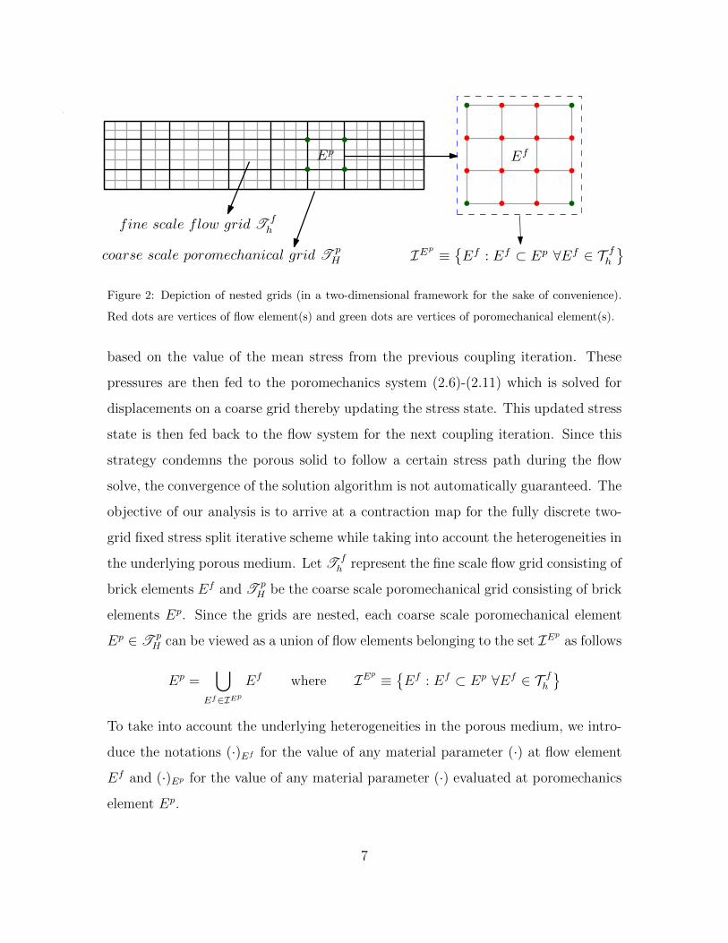
Figure 2: Depiction of nested grids (in a two-dimensional framework for the sake of convenience).

Red dots are vertices of flow element(s) and green dots are vertices of poromechanical element(s).

based on the value of the mean stress from the previous coupling iteration. These

pressures are then fed to the poromechanics system (2.6)-(2.11) which is solved for

displacements on a coarse grid thereby updating the stress state. This updated stress

state is then fed back to the flow system for the next coupling iteration. Since this

strategy condemns the porous solid to follow a certain stress path during the flow

solve, the convergence of the solution algorithm is not automatically guaranteed. The

objective of our analysis is to arrive at a contraction map for the fully discrete two-

grid fixed stress split iterative scheme while taking into account the heterogeneities in

the underlying porous medium. Let T fh represent the fine scale flow grid consisting of

brick elements Ef and T pH be the coarse scale poromechanical grid consisting of brick

elements Ep. Since the grids are nested, each coarse scale poromechanical element

Ep ∈ T pH can be viewed as a union of flow elements belonging to the set IEp as follows

Ep =⋃

Ef∈IEpEf where IEp ≡

Ef : Ef ⊂ Ep ∀Ef ∈ T fh

To take into account the underlying heterogeneities in the porous medium, we intro-

duce the notations (·)Ef for the value of any material parameter (·) at flow element

Ef and (·)Ep for the value of any material parameter (·) evaluated at poromechanics

element Ep.

7

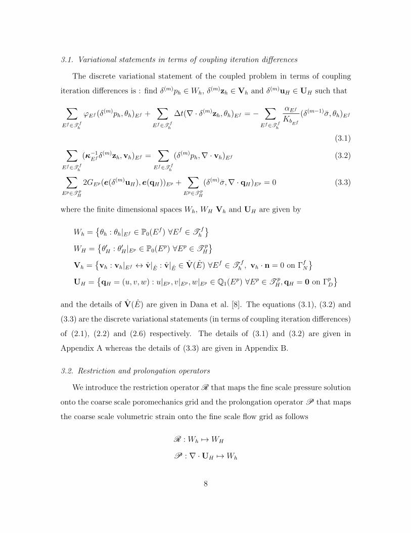
3.1. Variational statements in terms of coupling iteration differences

The discrete variational statement of the coupled problem in terms of coupling

iteration differences is : find δ(m)ph ∈ Wh, δ(m)zh ∈ Vh and δ(m)uH ∈ UH such that∑

Ef∈T fh

ϕEf (δ(m)ph, θh)Ef +

∑Ef∈T f

h

∆t(∇ · δ(m)zh, θh)Ef = −∑

Ef∈T fh

αEf

KbEf

(δ(m−1)σ, θh)Ef

(3.1)∑Ef∈T f

h

(κ−1Efδ(m)zh,vh)Ef =

∑Ef∈T f

h

(δ(m)ph,∇ · vh)Ef (3.2)

∑Ep∈T p

H

2GEp(e(δ(m)uH), e(qH))Ep +∑

Ep∈T pH

(δ(m)σ,∇ · qH)Ep = 0 (3.3)

where the finite dimensional spaces Wh, WH Vh and UH are given by

Wh =θh : θh|Ef ∈ P0(Ef ) ∀Ef ∈ T f

h

WH =

θ′H : θ′H |Ep ∈ P0(Ep) ∀Ep ∈ T p

H

Vh =

vh : vh|Ef ↔ v|E : v|E ∈ V(E) ∀Ef ∈ T f

h , vh · n = 0 on ΓfN

UH =qH = (u, v, w) : u|Ep , v|Ep , w|Ep ∈ Q1(Ep) ∀Ep ∈ T p

H ,qH = 0 on ΓpD

and the details of V(E) are given in Dana et al. [8]. The equations (3.1), (3.2) and

(3.3) are the discrete variational statements (in terms of coupling iteration differences)

of (2.1), (2.2) and (2.6) respectively. The details of (3.1) and (3.2) are given in

Appendix A whereas the details of (3.3) are given in Appendix B.

3.2. Restriction and prolongation operators

We introduce the restriction operator R that maps the fine scale pressure solution

onto the coarse scale poromechanics grid and the prolongation operator P that maps

the coarse scale volumetric strain onto the fine scale flow grid as follows

R : Wh 7→ WH

P : ∇ ·UH 7→ Wh

8

As a result, the mean stress is defined on the fine and coarse grids as

σ = KbEp εH − αEpRph (∀ Ep ∈ T pH) (3.4)

σ = KbEf

P εH − αEfph (∀ Ef ∈ T fh ) (3.5)

Theorem 3.1. In the presence of medium heterogeneities, the two-grid fixed stress

split iterative scheme in which the flow subproblem is resolved on a finer grid is a

contraction map with contraction constant γ and given by

∑Ef∈T f

h

‖δ(m)σ‖2Ef

KbEf

+

>0︷ ︸︸ ︷∑Ep∈T p

H

4GEp‖e(δ(m)uH)‖2Ep +

>0︷ ︸︸ ︷∑Ep∈T p

H

KbEp‖δ(m)εH‖2

Ep

+

>0︷ ︸︸ ︷∑Ef∈T f

h

2∆t‖κ−1/2

Efδ(m)zh‖2

Ef ≤

γ<1︷ ︸︸ ︷maxEf∈T f

h

(α2Ef

KbEf

MEf

+ α2Ef

) ∑Ef∈T f

h

‖δ(m−1)σ‖2Ef

KbEf

(3.6)

if the following conditions are satisfied

1. First condition∑Ef∈T f

h

αEf (Pδ(m)εH , δ(m)ph)Ef −

∑Ep∈T p

H

αEp(δ(m)εH ,Rδ(m)ph)Ep = 0

2. Second condition∑Ep∈T p

H

KbEp‖δ(m)εH‖2

Ep −∑

Ef∈T fh

KbEf‖Pδ(m)εH‖2

Ef ≥ 0

Proof. • Step 1: Flow equations

Testing (3.1) with θh ∈ Wh such that θh|Ef = δ(m)ph ∀ Ef ∈ T fh , we get∑

Ef∈T fh

ϕEf‖δ(m)ph‖2Ef +

∑Ef∈T f

h

∆t(∇ · δ(m)zh, δ(m)ph)Ef = −

∑Ef∈T f

h

αEf

KbEf

(δ(m−1)σ, δ(m)ph)Ef

(3.7)

Testing (3.2) with vh ∈ Vh such that vh|Ef ≡ δ(m)zh ∀ Ef ∈ T fh , we get∑

Ef∈T fh

‖κ−1/2

Efδ(m)zh‖2

Ef =∑

Ef∈T fh

(δ(m)ph,∇ · δ(m)zh)Ef (3.8)

9

From (3.7) and (3.8), we get∑Ef∈T f

h

ϕEf‖δ(m)ph‖2 +∑

Ef∈T fh

∆t‖κ−1/2

Efδ(m)zh‖2

Ef = −∑

Ef∈T fh

αEf

KbEf

(δ(m−1)σ, δ(m)ph)Ef

(3.9)

• Step 2: Invoking the Young’s inequality

Since the terms on the LHS of (3.9) are strictly positive, the RHS is also strictly

positive. We invoke the Young’s inequality for the RHS of (3.9) as follows

− αEf

KbEf

(δ(m−1)σ, δ(m)ph)Ef ≤1

2εEfK2bEf

‖δ(m−1)σ‖2Ef +

εEf

2‖αEf δ(m)ph‖2

Ef (∀ Ef ∈ T fh )

Since the above inequality is true for any εEf > 0, we choose εEf = 1α2EfϕEf to get

− αEf

KbEf

(δ(m−1)σ, δ(m)ph)Ef ≤α2Ef

2KbEfϕEf

‖δ(m−1)σ‖2Ef

KbEf

+ϕEf

2‖δ(m)ph‖2

Ef (∀ Ef ∈ T fh )

In lieu of the above, (3.9) is written as∑Ef∈T f

h

ϕEf‖δ(m)ph‖2Ef +

∑Ef∈T f

h

∆t‖κ−1/2

Efδ(m)zh‖2

Ef

≤∑

Ef∈T fh

α2Ef

2KbEfϕEf

‖δ(m−1)σ‖2Ef

KbEf

+∑

Ef∈T fh

ϕEf

2‖δ(m)ph‖2

Ef

which can also be written as∑Ef∈T f

h

ϕEf

2‖δ(m)ph‖2 +

∑Ef∈T f

h

∆t‖κ−1/2

Efδ(m)zh‖2

Ef ≤∑

Ef∈T fh

α2Ef

2KbEfϕEf

‖δ(m−1)σ‖2Ef

KbEf

which, after noting that ϕEf ≡(

1MEf

+α2Ef

KbEf

)>

α2Ef

KbEf

, can also be written as

∑Ef∈T f

h

α2Ef

KbEf

‖δ(m)ph‖2Ef +

∑Ef∈T f

h

2∆t‖κ−1/2

Efδ(m)zh‖2

Ef ≤∑

Ef∈T fh

α2Ef

KbEfϕEf

‖δ(m−1)σ‖2Ef

KbEf

(3.10)

10

• Step 3: Poromechanics equations

Testing (3.3) with qH ∈ QH such that q|Ep = 2δ(m)uH ∀ Ep ∈ T pH and noting that

∇ · δ(m)uH ≡ δ(m)εH , we get∑Ep∈T p

H

4GEp‖e(δ(m)uH)‖2Ep +

∑Ep∈T p

H

2(δ(m)σ, δ(m)εH)Ep = 0 (3.11)

Further, from (3.4), we note that δ(m)σ = KbEpδ(m)εH − αEpRδ(m)ph ∀ Ep ∈ T p

H . As

a result, (3.11) is written as∑Ep∈T p

H

4GEp‖e(δ(m)uH)‖2Ep +

∑Ep∈T p

H

2KbEp‖δ(m)εH‖2

Ep −∑

Ep∈T pH

2αEp(δ(m)εH ,Rδ(m)ph)Ep = 0

(3.12)

• Step 4: Combining flow and poromechanics equations

Adding (3.10) and (3.12), we get∑Ef∈T f

h

α2Ef

KbEf

‖δ(m)ph‖2Ef +

∑Ef∈T f

h

2∆t‖κ−1/2

Efδ(m)zh‖2

Ef

+∑

Ep∈T pH

4GEp‖e(δ(m)uH)‖2Ep +

∑Ep∈T p

H

2KbEp‖δ(m)εH‖2

Ep

−∑

Ep∈T pH

2αEp(δ(m)εH ,Rδ(m)ph)Ep ≤

∑Ef∈T f

h

α2Ef

KbEfϕEf

‖δ(m−1)σ‖2Ef

KbEf

(3.13)

Now, from (3.5), we note that

‖δ(m)σ‖2Ef = α2

Ef‖δ(m)ph‖2

Ef +K2bEf‖Pδ(m)εH‖2

Ef − 2KbEfαEf (Pδ(m)εH , δ

(m)ph)Ef

(∀ Ef ∈ T fh )

which implies that

α2Ef

KbEf

‖δ(m)ph‖2Ef =

‖δ(m)σ‖2Ef

KbEf

−KbEf‖Pδ(m)εH‖2

Ef + 2αEf (Pδ(m)εH , δ(m)ph)Ef

(∀ Ef ∈ T fh ) (3.14)

11

Substituting (3.14) in (3.13), we get

∑Ef∈T f

h

‖δ(m)σ‖2Ef

KbEf

+

>0︷ ︸︸ ︷∑Ep∈T p

H

4GEp‖e(δ(m)uH)‖2Ep +

>0︷ ︸︸ ︷∑Ep∈T p

H

KbEp‖δ(m)εH‖2

Ep

+

[ Set = 0 to obtain expressions for KbEp ∀ Ep∈T pH and Pδ(m)εH ∀ Ef∈T f

h︷ ︸︸ ︷∑Ef∈T f

h

2αEf (Pδ(m)εH , δ(m)ph)Ef −

∑Ep∈T p

H

2αEp(δ(m)εH ,Rδ(m)ph)Ep

]

+

[ Turns out to be ≥0 in lieu of Cauchy−Schwartz inequality︷ ︸︸ ︷∑Ep∈T p

H

KbEp‖δ(m)εH‖2

Ep −∑

Ef∈T fh

KbEf‖Pδ(m)εH‖2

Ef

]

+

>0︷ ︸︸ ︷∑Ef∈T f

h

2∆t‖κ−1/2

Efδ(m)zh‖2

Ef ≤ γ∑

Ef∈T fh

‖δ(m−1)σ‖2Ef

KbEf

(3.15)

The statement (3.15) is a contraction map in a sense that

∑Ef∈T f

h

‖δ(0)σ‖2Ef

KbEf

>∑

Ef∈T fh

‖δ(1)σ‖2Ef

KbEf

>∑

Ef∈T fh

‖δ(2)σ‖2Ef

KbEf

> ...

with contraction constant γ given by

γ ≡ maxEf∈T f

h

(α2Ef

KbEfϕEf

)= max

Ef∈T fh

(α2Ef

KbEf

MEf

+ α2Ef

)< 1

provided the following are true∑Ef∈T f

h

αEf (Pδ(m)εH , δ(m)ph)Ef −

∑Ep∈T p

H

αEp(δ(m)εH ,Rδ(m)ph)Ep = 0 (3.16)

∑Ep∈T p

H

KbEp‖δ(m)εH‖2

Ep −∑

Ef∈T fh

KbEf‖Pδ(m)εH‖2

Ef ≥ 0 (3.17)

The objective now is to satisfy the conditions (3.16) and (3.17) for the convergence

of the two-grid fixed stress split scheme.

12

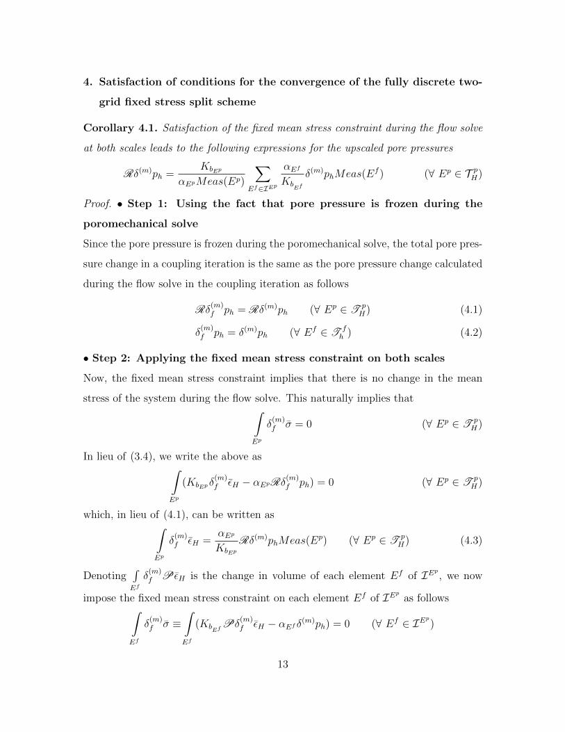
4. Satisfaction of conditions for the convergence of the fully discrete two-

grid fixed stress split scheme

Corollary 4.1. Satisfaction of the fixed mean stress constraint during the flow solve

at both scales leads to the following expressions for the upscaled pore pressures

Rδ(m)ph =KbEp

αEpMeas(Ep)

∑Ef∈IEp

αEf

KbEf

δ(m)phMeas(Ef ) (∀ Ep ∈ T pH)

Proof. • Step 1: Using the fact that pore pressure is frozen during the

poromechanical solve

Since the pore pressure is frozen during the poromechanical solve, the total pore pres-

sure change in a coupling iteration is the same as the pore pressure change calculated

during the flow solve in the coupling iteration as follows

Rδ(m)f ph = Rδ(m)ph (∀ Ep ∈ T p

H) (4.1)

δ(m)f ph = δ(m)ph (∀ Ef ∈ T f

h ) (4.2)

• Step 2: Applying the fixed mean stress constraint on both scales

Now, the fixed mean stress constraint implies that there is no change in the mean

stress of the system during the flow solve. This naturally implies that∫Ep

δ(m)f σ = 0 (∀ Ep ∈ T p

H)

In lieu of (3.4), we write the above as∫Ep

(KbEpδ(m)f εH − αEpRδ

(m)f ph) = 0 (∀ Ep ∈ T p

H)

which, in lieu of (4.1), can be written as∫Ep

δ(m)f εH =

αEp

KbEpRδ(m)phMeas(Ep) (∀ Ep ∈ T p

H) (4.3)

Denoting∫Efδ

(m)f P εH is the change in volume of each element Ef of IEp , we now

impose the fixed mean stress constraint on each element Ef of IEp as follows∫Ef

δ(m)f σ ≡

∫Ef

(KbEf

Pδ(m)f εH − αEf δ(m)ph) = 0 (∀ Ef ∈ IEp)

13

which, in lieu of (4.2), can be written as∫Ef

Pδ(m)f εH =

αEf

KbEf

δ(m)phMeas(Ef ) (∀ Ef ∈ T fh ) (4.4)

• Step 3: Using the fact that the change in volume measured on both

scales should be identical

The term∫Epδ

(m)f εH is the change in volume of Ep during the flow solve in the (m +

1)th coupling iteration. This naturally equates the sum of corresponding changes in

volumes of the elements of IEp as follows∫Ep

δ(m)f εH ≡

∑Ef∈IEp

∫Ef

Pδ(m)f εH (∀ Ep ∈ T p

H) (4.5)

From (4.4) and (4.5), we get∫Ep

δ(m)f εH =

∑Ef∈IEp

αEf

KbEf

δ(m)phMeas(Ef ) (∀ Ep ∈ T pH) (4.6)

From (4.3) and (4.6), we get∑Ef∈IEp

αEf

KbEf

δ(m)phMeas(Ef ) =αEp

KbEpRδ(m)phMeas(Ep) (∀ Ep ∈ T p

H)

which results in

Rδ(m)ph =KbEp

αEpMeas(Ep)

∑Ef∈IEp

αEf

KbEf

δ(m)phMeas(Ef ) (∀ Ep ∈ T pH) (4.7)

Corollary 4.2. Satisfaction of the condition (3.16) leads to the following expressions

for the effective bulk moduli for the coarse scale poromechanical solve

KbEp =1∑

Ef∈IEp1

KbEf

Meas(Ef )Meas(Ep)

(∀ Ep ∈ T pH)

and the following expressions for the downscaled volumetric strains

Pδ(m)εH =KbEp

KbEf

1

Meas(Ep)

∫Ep

δ(m)εH (∀ Ef ∈ IEp ∀ Ep ∈ T pH)

14

Proof. • Step 1: Recasting the first term on LHS of (3.16)

We start by modifying the first term on LHS of (3.16) as follows∑Ef∈T f

h

αEf (Pδ(m)εH , δ(m)ph)Ef =

∑Ef∈T f

h

αEf δ(m)phPδ(m)εHMeas(Ef ) (4.8)

where we note that δ(m)ph ∈ Wh. Since a flow element Ef ∈ T fh in uniquely associated

with a poromechanical element Ep via IEp , we can write∑Ef∈T f

h

αEf δ(m)phPδ(m)εHMeas(Ef ) =

∑Ep∈T p

H

∑Ef∈IEp

αEf δ(m)phPδ(m)εHMeas(Ef )

In lieu of the above, we write (4.8) as∑Ef∈T f

h

αEf (Pδ(m)εH , δ(m)ph)Ef =

∑Ep∈T p

H

∑Ef∈IEp

αEf δ(m)phPδ(m)εHMeas(Ef ) (4.9)

• Step 2: Recasting the second term on LHS of (3.16)

Next, we modify the second term on LHS of (3.16) as follows∑Ep∈T p

H

αEp(δ(m)εH ,Rδ(m)ph)Ep ≡

∑Ep∈T p

H

2αEpRδ(m)ph

∫Ep

δ(m)εH (4.10)

where we note that Rδ(m)ph ∈ WH . In lieu of (4.9) and (4.10), the first condition

given by (3.16) is rewritten as∑Ep∈T p

H

∑Ef∈IEp

αEf δ(m)phPδ(m)εHMeas(Ef ) =

∑Ep∈T p

H

αEpRδ(m)ph

∫Ep

δ(m)εH (4.11)

• Step 3: Substituting the expression for upscaled pore pressures

Substituting the expression (4.7) for the upscaled pore pressure in (4.11), we get∑Ep∈T p

H

∑Ef∈IEp

αEf δ(m)phPδ(m)εHMeas(Ef )

=∑

Ep∈T pH

αEp

Rδ(m)ph︷ ︸︸ ︷KbEp

αEpMeas(Ep)

∑Ef∈IEp

αEf

KbEf

δ(m)phMeas(Ef )

∫Ep

δ(m)εH

15

which implies that∑Ep∈T p

H

∑Ef∈IEp

(Pδ(m)εH −

KbEp

KbEf

1

Meas(Ep)

∫Ep

δ(m)εH

)αEf δ

(m)phMeas(Ef ) = 0

which, in lieu of the linear independence of the basis ph (∀ Ef ∈ T fh ) of the pressure

space on the fine scale flow grid, implies that

Pδ(m)εH −KbEp

KbEf

1

Meas(Ep)

∫Ep

δ(m)εH = 0 (∀ Ef ∈ IEp ∀ Ep ∈ T pH)

implying that

Pδ(m)εH =KbEp

KbEf

1

Meas(Ep)

∫Ep

δ(m)εH (∀ Ef ∈ IEp ∀ Ep ∈ T pH) (4.12)

• Step 4: Using the fact that the change in volume measured on both

scales should be identical

The change in volume of Ep over the (m+ 1)th coupling iteration equates the sum of

corresponding changes in volumes of the elements of IEp as follows∫Ep

δ(m)εH =∑

Ef∈IEp

∫Ef

Pδ(m)εH =∑

Ef∈IEpPδ(m)εHMeas(Ef ) (∀ Ep ∈ T p

H)

(4.13)

In lieu of (4.12) and (4.13), we get∫Ep

δ(m)εH =

∫Ep

δ(m)εH∑

Ef∈IEp

KbEp

KbEf

Meas(Ef )

Meas(Ep)(∀ Ep ∈ T p

H)

which finally leads to

1

KbEp=

∑Ef∈IEp

1

KbEf

Meas(Ef )

Meas(Ep)(∀ Ep ∈ T p

H) (4.14)

Corollary 4.3. The Cauchy-Schwartz inequality, along with the obtained expressions

for effective coarse scale bulk moduli (4.14) and downscaled volumetric strains (4.12),

guarantees the satisfaction of the condition (3.17).

16

Proof. • Step 1: Recasting (3.17) in lieu of (4.12) and (4.14)

The condition (3.17) given by∑Ep∈T p

H

KbEp‖δ(m)εH‖2

Ep −∑

Ef∈T fh

KbEf‖Pδ(m)εH‖2

Ef ≥ 0

can be written as∑Ep∈T p

H

KbEp‖δ(m)εH‖2

Ep −∑

Ef∈T fH

KbEf|Pδ(m)εH |2Meas(Ef ) ≥ 0

which can also be written as∑Ep∈T p

H

[KbEp‖δ

(m)εH‖2Ep −

∑Ef∈IEp

KbEf|Pδ(m)εH |2Meas(Ef )

]≥ 0

which, in lieu of (4.12), can also be written as

∑Ep∈T p

H

[KbEp‖δ

(m)εH‖2Ep −

∑Ef∈IEp

KbEf

|Pδ(m)εH |2︷ ︸︸ ︷(KbEp

KbEf

1

Meas(Ep)

∫Ep

δ(m)εH

)2

Meas(Ef )

]≥ 0

which can also be written as∑Ep∈T p

H

[KbEp‖δ

(m)εH‖2Ep −

KbEp

Meas(Ep)

(∫Ep

|δ(m)εH |)2

KbEp

∑Ef∈IEp

1

KbEf

Meas(Ef )

Meas(Ep)

]≥ 0

which, in lieu of (4.14), can be written as

∑Ep∈T p

H

[KbEp‖δ

(m)εH‖2Ep −

KbEp

Meas(Ep)

(∫Ep

|δ(m)εH |)2

KbEp1

KbEp

]≥ 0

which can be finally written as∑Ep∈T p

H

[KbEp‖δ

(m)εH‖2Ep −

KbEp

Meas(Ep)

(∫Ep

|δ(m)εH |)2]≥ 0 (4.15)

• Step 2: Applying the Cauchy-Schwartz inequality

The Cauchy-Schwartz inequality (see Oden and Demkowicz [16]) states that if S

17

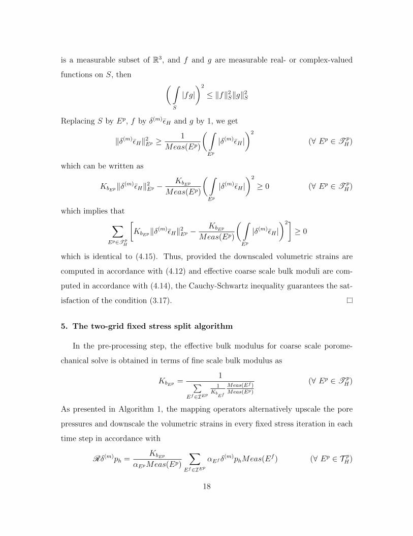
is a measurable subset of R3, and f and g are measurable real- or complex-valued

functions on S, then (∫S

|fg|)2

≤ ‖f‖2S‖g‖2

S

Replacing S by Ep, f by δ(m)εH and g by 1, we get

‖δ(m)εH‖2Ep ≥

1

Meas(Ep)

(∫Ep

|δ(m)εH |)2

(∀ Ep ∈ T pH)

which can be written as

KbEp‖δ(m)εH‖2

Ep −KbEp

Meas(Ep)

(∫Ep

|δ(m)εH |)2

≥ 0 (∀ Ep ∈ T pH)

which implies that∑Ep∈T p

H

[KbEp‖δ

(m)εH‖2Ep −

KbEp

Meas(Ep)

(∫Ep

|δ(m)εH |)2]≥ 0

which is identical to (4.15). Thus, provided the downscaled volumetric strains are

computed in accordance with (4.12) and effective coarse scale bulk moduli are com-

puted in accordance with (4.14), the Cauchy-Schwartz inequality guarantees the sat-

isfaction of the condition (3.17).

5. The two-grid fixed stress split algorithm

In the pre-processing step, the effective bulk modulus for coarse scale porome-

chanical solve is obtained in terms of fine scale bulk modulus as

KbEp =1∑

Ef∈IEp1

KbEf

Meas(Ef )Meas(Ep)

(∀ Ep ∈ T pH)

As presented in Algorithm 1, the mapping operators alternatively upscale the pore

pressures and downscale the volumetric strains in every fixed stress iteration in each

time step in accordance with

Rδ(m)ph =KbEp

αEpMeas(Ep)

∑Ef∈IEp

αEf δ(m)phMeas(Ef ) (∀ Ep ∈ T pH)

18

Algorithm 1 Two-grid fixed-stress split iterative scheme for consolidation in hetero-

geneous poroelastic medium

For each time tn

repeat . Fixed-stress iteration # (m+ 1)

Solve the flow equations for pm+1,n+1h and zm+1,n+1

h

Compute δ(m)ph ≡ pm+1,n+1h − pm,n+1

h

Obtain Rδ(m)ph . Upscale pore pressures

Obtain Rpm+1,n+1h ≡ Rpm,n+1

h + Rδ(m)ph

Using Rpm+1,n+1h , solve the poromechanics equations for um+1,n+1

H

Compute δ(m)εH ≡ δ(m)∇ · uH = ∇ · um+1,n+1H −∇ · um,n+1

H

Obtain Pδ(m)εH . Downscale volumetric strains

Obtain P εm+1,n+1H ≡Pδ(m)εH + P εm,n+1

H

Obtain δ(m)σ = KbEf

Pδ(m)εH − αEf δ(m)ph

until Stopping criterion ∥∥∥∥ζm+1c − ζm+1

p

ζm+1c

∥∥∥∥L∞≤ TOL

Increment tn → tn+1

Pδ(m)εH =KbEp

KbEf

1

Meas(Ep)

∫Ep

δ(m)εH (∀ Ef ∈ IEp ∀ Ep ∈ T pH)

5.1. Convergence criterion

The variation in fluid content δ(m)f ζ measured on the coarse scale poromechanical

grid during the flow solve in the (m+ 1)th coupling iteration at any time step is

δ(m)f ζ =

1

MEpRδ

(m)f ph + αEpδ

(m)f εH = ζm+1

p − ζm (∀Ep ∈ T pH) (5.1)

where ζm is the fluid content at the end of the previous or mth coupling iteration and

ζm+1p serves as the predictor to the fluid content at the end of the current or (m+1)th

coupling iteration. The variation in fluid content δ(m)ζ measured on the coarse scale

poromechanical grid over the (m + 1)th coupling iteration (including the flow solve

19

and poromechanics solve) at any time step is

δ(m)ζ =1

MEpRδ(m)ph + αEpδ

(m)εH = ζm+1c − ζm (∀Ep ∈ T p

H) (5.2)

where ζm+1c serves as the corrector to ζm+1

p . Subtracting (5.1) from (5.2) and noting

that Rδ(m)f ph ≡ Rδ(m)ph since the pore pressure is frozen during the poromechanical

solve, we get

ζm+1c − ζm+1

p = αEpδ(m)εH − αEpδ(m)

f εH = αEp(εm+1Hc− εm+1

Hp) (∀Ep ∈ T p

H)

which implies that the difference between the predicted value and the corrected value

of the fluid content measured on the coarse scale poromechanical grid at the end of

the (m+ 1)th coupling iteration is equal to the difference between the predicted value

(εm+1Hp

) and the corrected value (εm+1Hc

) of the volumetric strain measured on the coarse

scale poromechanical grid at the end of the (m+ 1)th coupling iteration scaled by the

Biot constant. In lieu of the above, the stopping criterion for coupling iterations at

any time step is ∥∥∥∥ζm+1c − ζm+1

p

ζm+1c

∥∥∥∥L∞≤ TOL

Acknowledgements

The first author Saumik Dana would like to thank Gurpreet Singh (Research

Associate at Center for Subsurface Modeling) for inputs during the course of the

rendition of this theoretical work.

Appendix A. Discrete variational statements for the flow subproblem in

terms of coupling iteration differences

Before arriving at the discrete variational statement of the flow model, we impose

the fixed mean stress constraint on the strong form of the mass conservation equation

(2.1). Invoking the relation for the total mean stress σ = Kbε− αp, we get

∂

∂t

(1

Mp+ α

(σ + αp

Kb

))+∇ · z = q

20

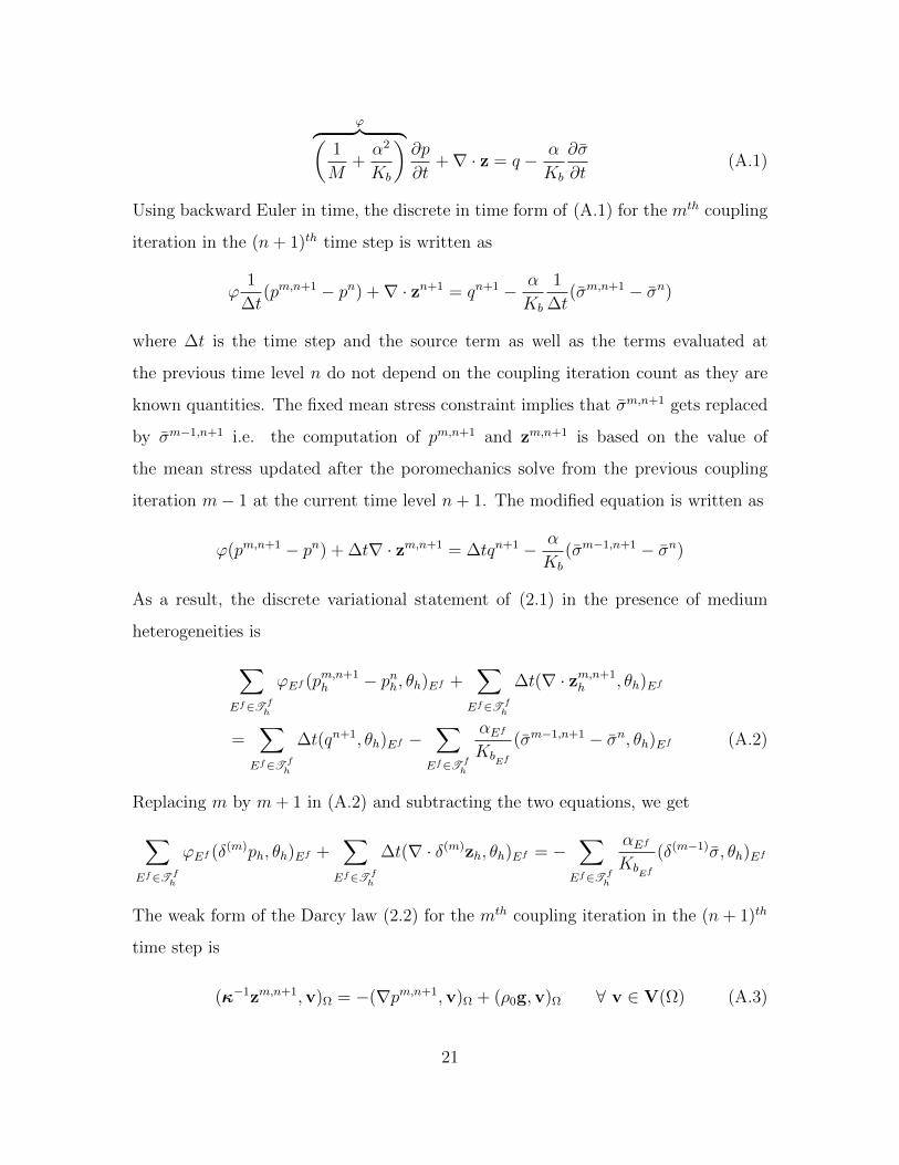
ϕ︷ ︸︸ ︷(1

M+α2

Kb

)∂p

∂t+∇ · z = q − α

Kb

∂σ

∂t(A.1)

Using backward Euler in time, the discrete in time form of (A.1) for the mth coupling

iteration in the (n+ 1)th time step is written as

ϕ1

∆t(pm,n+1 − pn) +∇ · zn+1 = qn+1 − α

Kb

1

∆t(σm,n+1 − σn)

where ∆t is the time step and the source term as well as the terms evaluated at

the previous time level n do not depend on the coupling iteration count as they are

known quantities. The fixed mean stress constraint implies that σm,n+1 gets replaced

by σm−1,n+1 i.e. the computation of pm,n+1 and zm,n+1 is based on the value of

the mean stress updated after the poromechanics solve from the previous coupling

iteration m− 1 at the current time level n+ 1. The modified equation is written as

ϕ(pm,n+1 − pn) + ∆t∇ · zm,n+1 = ∆tqn+1 − α

Kb

(σm−1,n+1 − σn)

As a result, the discrete variational statement of (2.1) in the presence of medium

heterogeneities is∑Ef∈T f

h

ϕEf (pm,n+1h − pnh, θh)Ef +

∑Ef∈T f

h

∆t(∇ · zm,n+1h , θh)Ef

=∑

Ef∈T fh

∆t(qn+1, θh)Ef −∑

Ef∈T fh

αEf

KbEf

(σm−1,n+1 − σn, θh)Ef (A.2)

Replacing m by m+ 1 in (A.2) and subtracting the two equations, we get∑Ef∈T f

h

ϕEf (δ(m)ph, θh)Ef +

∑Ef∈T f

h

∆t(∇ · δ(m)zh, θh)Ef = −∑

Ef∈T fh

αEf

KbEf

(δ(m−1)σ, θh)Ef

The weak form of the Darcy law (2.2) for the mth coupling iteration in the (n+ 1)th

time step is

(κ−1zm,n+1,v)Ω = −(∇pm,n+1,v)Ω + (ρ0g,v)Ω ∀ v ∈ V(Ω) (A.3)

21

where V(Ω) is given by

V(Ω) ≡ H(div,Ω) ∩v : v · n = 0 on ΓfN

We use the divergence theorem to evaluate the first term on RHS of (A.3) as follows

(∇pm,n+1,v)Ω = (∇, pm,n+1v)Ω − (pm,n+1,∇ · v)Ω

= (pm,n+1,v · n)∂Ω − (pm,n+1,∇ · v)Ω = (g,v · n)ΓfD− (pm,n+1,∇ · v)Ω (A.4)

where we invoke v · n = 0 on ΓfN . In lieu of (A.3) and (A.4), we get

(κ−1zm,n+1,v)Ω = −(g,v · n)ΓfD+ (pm,n+1,∇ · v)Ω + (ρ0g,v)Ω

As a result, the discrete variational statement of (2.2) in the presence of medium

heterogeneities is ∑Ef∈T f

h

(κ−1Ef

zm,n+1h ,vh)Ef −

∑Ef∈T f

h

(pm,n+1h ,∇ · vh)Ef

=∑

Ef∈T fh

(ρ0g,vh)Ef −∑

Ef∈T fh

(g,vh · n)∂Ef∩ΓfD(A.5)

Replacing m by m+ 1 in (A.5) and subtracting the two equations, we get∑Ef∈T f

h

(κ−1Efδ(m)zh,vh)Ef =

∑Ef∈T f

h

(δ(m)ph,∇ · vh)Ef

Appendix B. Discrete variational statement for the poromechanics sub-

problem in terms of coupling iteration differences

The weak form of the linear momentum balance (2.6) is given by

(∇ · σ,q)Ω + (f · q)Ω = 0 (∀ q ∈ U(Ω)) (B.1)

where U(Ω) is given by

U(Ω) ≡q = (u, v, w) : u, v, w ∈ H1(Ω),q = 0 on ΓpD

22

where Hm(Ω) is defined, in general, for any integer m ≥ 0 as

Hm(Ω) ≡w : Dαw ∈ L2(Ω) ∀|α| ≤ m

,

where the derivatives are taken in the sense of distributions and given by

Dαw =∂|α|w

∂xα11 ..∂x

αnn

, |α| = α1 + · · ·+ αn,

We know from tensor calculus that

(∇ · σ,q) ≡ (∇,σq)− (σ,∇q) (B.2)

Further, using the divergence theorem and the symmetry of σ, we arrive at

(∇,σq)Ω ≡ (q,σn)∂Ω (B.3)

We decompose ∇q into a symmetric part (∇q)s ≡ 12

(∇q + (∇q)T

)≡ ε(q) and

skew-symmetric part (∇q)ss and note that the contraction between a symmetric and

skew-symmetric tensor is zero to obtain

σ : ∇q ≡ σ : (∇q)s +:

0σ : (∇q)ss = σ : ε(q) (B.4)

From (B.1), (B.2), (B.3) and (B.4), we get

(σn,q)∂Ω − (σ, ε(q))Ω + (f ,q)Ω = 0

which, after invoking the boundary condition σn = t on ΓpN results in

(t,q)ΓpN− (σ, ε(q))Ω + (f ,q)Ω = 0 (B.5)

The stress tensor σ and strain tensor ε(q) are written as

σ = s+1

3tr(σ)I = s+ σI; ε(q) = e(q) +

1

3tr(ε(q))I = e(q) +

1

3ε(q)I

where s is the deviatoric stress tensor, e(q) is the deviatoric strain tensor and σ is

the mean stress. Using the above relations, we can write

σ : ε(q) =(s+ σI

):(e(q) +

1

3ε(q)I

)= s : e(q) + s :

1

3ε(q)I + σI : e(q) + σI :

1

3ε(q)I

23

= s : e(q) +1

3ε(q)

*0tr(s) + σ

:0tr(e(q)) + 3σ

1

3ε(q) = s : e(q) + σε(q) (B.6)

where we note that the contraction of any second order tensor with the identity tensor

I is equal to the trace of the tensor and further, the trace of a deviatoric tensor is

zero resulting in tr(s) = 0 and tr(e(q)) = 0. Substituting (B.6) in (B.5), we get

(t,q)ΓpN− (s, e(q))Ω − (σ, ε(q))Ω + (f ,q)Ω = 0 (B.7)

The deviatoric strain tensor is obtained as

s = σ − 1

3tr(σ)I = σ0 + λεI + 2Gε− α(p− p0)I− 1

3tr(σ0 + λεI + 2Gε− α(p− p0)I

)I

= s0 + 2G(ε− 1

3tr(ε)I

)= s0 + 2Ge (B.8)

Substituting (B.8) in (B.7), we get

(t,q)ΓpN− (s0, e(q))Ω − (2Ge, e(q))Ω − (σ, ε(q))Ω + (f ,q)Ω = 0

As a result, the discrete variational statement of the linear momentum balance (2.6)

for the mth coupling iteration in the (n + 1)th time step in the presence of medium

heterogeneities is written as∑Ep∈T p

H

2GEp(e(um,n+1H ), e(qH))Ep +

∑Ep∈T p

H

(σm,n+1,∇ · qH)Ep

=∑

Ep∈T pH

(f ,qH) +∑

Ep∈T pH

(t,qH)∂Ep∩ΓpN−∑

Ep∈T pH

(s0, e(qH))Ep (B.9)

Replacing m by m+ 1 in (B.9) and subtracting the two equations, we get∑Ep∈T p

H

2GEp(e(δ(m)uH), e(qH))Ep +∑

Ep∈T pH

(δ(m)σ,∇ · qH)Ep = 0

References

[1] Y. Abousleiman, A. H. D. Cheng, L. Cui, E. Detournay, and J. C. Roegiers.

Mandel’s problem revisited. Geotechnique, 46(2):187–195, 1996.

24

[2] T. Almani, K. Kumar, and M. F. Wheeler. Convergence analysis of single rate

and multirate fixed stress split iterative coupling schemes in heterogeneous poroe-

lastic media. ICES REPORT 17-23, The University of Texas at Austin, 2017.

[3] F. Armero and J. C. Simo. A new unconditionally stable fractional step method

for non-linear coupled thermomechanical problems. International Journal for

Numerical Methods in Engineering, 35(4):737–766, 1992.

[4] M. A. Biot. General theory of three dimensional consolidation. Journal of Applied

Physics, 12:155–164, 1941.

[5] M. A. Biot and D. G. Willis. The elastic coefficients of the theory of consolidation.

Journal of Applied Mechanics, 24:594–601, 1957.

[6] N. Castelletto, J. A. White, and H. A. Tchelepi. Accuracy and convergence

properties of the fixed-stress iterative solution of two-way coupled poromechanics.

International Journal for Numerical and Analytical Methods in Geomechanics,

39(14):1593–1618, 2015.

[7] O. Coussy. Poromechanics. Wiley, 2nd edition, 2004.

[8] S. Dana, B. Ganis, and M. F. Wheeler. A multiscale fixed stress split iterative

scheme for coupled flow and poromechanics in deep subsurface reservoirs. Journal

of Computational Physics, 352:1–22, 2018.

[9] E. Detournay and A. H. D. Cheng. Fundamentals of poroelasticity. In Com-

prehensive Rock Engineering: Principles, Practice and Projects, volume 2, pages

113–171. Pergamon Press, 1993.

[10] C. A. Felippa, K. C. Park, and C. Farhat. Partitioned analysis of coupled me-

chanical systems. Computer Methods in Applied Mechanics and Engineering, 190

(24):3247–3270, 2001.

25

[11] J. Geertsma. The effect of fluid pressure decline on volumetric changes of porous

rocks. SPE, 210:331–340, 1957.

[12] J. Kim, H. A. Tchelepi, and R. Juanes. Stability, accuracy and efficiency of

sequential methods for coupled flow and geomechanics. SPE Journal, 16(2):

249–262, 2011.

[13] J. Mandel. Consolidation des sols (etude mathematique)*. Geotechnique, 3(7):

287–299, 1953.

[14] A. Mikelic and M. F. Wheeler. Convergence of iterative coupling for coupled

flow and geomechanics. Computational Geosciences, 17(3):455–461, 2013.

[15] A. Nur and J. D. Byerlee. An exact effective stress law for elastic deformation

of rock with fluids. Journal of Geophysical Research, 76(26):6414–6419, 1971.

[16] J. T. Oden and L. Demkowicz. Applied Functional Analysis. Chapman and Hall,

2nd edition, 2010.

[17] J. R. Rice and M. P. Cleary. Some basic stress diffusion solutions for fluid-

saturated elastic porous media with compressible constituents. Reviews of Geo-

physics, 14(2):227–241, 1976.

[18] B. A. Schrefler, L. Simoni, and E. Turska. Standard staggered and staggered

newton schemes in thermo-hydro-mechanical problems. Computer Methods in

Applied Mechanics and Engineering, 144(1-2):93–109, 1997.

[19] E. Turska and B. A. Schrefler. On convergence conditions of partitioned solution

procedures for consolidation problems. Computer Methods in Applied Mechanics

and Engineering, 106(1-2):51–63, 1993.

[20] J. A. White, N. Castelletto, and H. A. Tchelepi. Block-partitioned solvers for

coupled poromechanics: A unified framework. Computer Methods in Applied

Mechanics and Engineering, 303:55–74, 2016.

26

View publication statsView publication stats