ICES REPORT 14-26

August 2014

Single-variable formulations and isogeometricdiscretizations for shear deformable beams

by

J. Kiendl, F. Auricchio, T.J.R. Hughes, A. Reali

The Institute for Computational Engineering and SciencesThe University of Texas at AustinAustin, Texas 78712

Reference: J. Kiendl, F. Auricchio, T.J.R. Hughes, A. Reali, "Single-variable formulations and isogeometricdiscretizations for shear deformable beams ," ICES REPORT 14-26, The Institute for Computational Engineeringand Sciences, The University of Texas at Austin, August 2014.

Single-variable formulations and isogeometricdiscretizations for shear deformable beams

J. Kiendla,∗, F. Auricchioa, T.J.R. Hughesb, A. Realia

aDepartment of Civil Engineering and Architecture, University of Pavia, Italy

bInstitute for Computational Engineering and Sciences, University of Texas at Austin, USA

Abstract

We present numerical formulations of Timoshenko beams with only one unknown,the bending displacement, and it is shown that all variables of the beam problem canbe expressed in terms of it and its derivatives. We develop strong and weak formsof the problem. The strong form of the problem involves the fourth derivative ofthe bending displacement, whereas the symmetric weak form involves, somewhatsurprisingly, third and second derivatives. Based on these, we develop isogeometriccollocation and Galerkin formulations, that are completely locking-free and involveonly half the degrees of freedom compared to standard Timoshenko beam formula-tions. Several numerical tests are presented to demonstrate the performance of theproposed formulations.

Keywords: Timoshenko beam, shear-deformable, locking-free, isogeometric,collocation, finite elements

1. Introduction

The two major theories for structural analysis of beams are the Bernoulli-Euler andTimoshenko theories. In the Bernoulli-Euler theory cross sections are assumed toremain straight and normal to the mid-axis during deformation, which implies thatthe rotation of a cross section can be obtained from the derivative of the deflection.This assumption corresponds to neglecting shear deformation and is valid for thinbeams. In the Timoshenko theory cross sections are also assumed to remain straightbut not necessarily normal to the mid-axis, which accommodates shear deformation.As a consequence, rotation and deflection are typically considered independent vari-ables.

∗Corresponding authorEmail address: josef.kiendl@unipv.it (J. Kiendl)

Preprint submitted to Computer Methods in Applied Mechanics and Engineering June 17, 2014

In this paper, we present a relation between deflection and rotation for Timoshenkobeams which leads to formulations with only one variable. In particular, we splitthe displacement into a bending and a shear part, and show that these two parts arerelated, which allows expressing all derived variables, such as rotation and shearstrain, in terms of the bending displacement. The idea of splitting the displacementof Timoshenko beams into a bending and a shear part can be found in papers fromthe early days of beam finite elements; see, for example, Kapur [13]. In [13],however, no relation between the bending and shear part is established. Instead,displacement and rotation are discretized independently for both the bending andshear part, resulting in four unknown fields, which eventually yields a formulationwith twice the number of degrees of freedom compared to a standard formulation.

In the present paper, we derive a single differential equation for the Timoshenkobeam problem with the bending displacement as the only unknown. This differ-ential equation is form-identical to the one for a Bernoulli-Euler beam model butfully accounts for shear deformation. Similar approaches have been presented byLi [16] and Falsone et al. [8]. In both papers, the Timoshenko beam problem isreduced to a single equation in terms of one variable. These approaches do notutilize the split into bending and shear terms, but the resulting equations are es-sentially equivalent to the one presented in this paper. However, Li [16] does notdevelop a weak formulation and does not pursue a discrete formulation, or numeri-cal calculations. Falsone et al. [8] develop a weak form and a corresponding finiteelement formulation, but their weak form is not symmetric and produces boundaryterms at element level, which need to be coupled between elements. Furthermore,an additional change of basis at element boundaries is required in order to guaranteecontinuity of the displacement between elements. In the present paper, we establisha weak form which is both symmetric and without boundary terms at element level,but involves both second and third derivatives of the bending displacement. Due tothe isogeometric basis functions adopted in this paper, suitable degree and conti-nuity of the bending displacement are automatically guaranteed. In addition to theGalerkin formulation, we develop an isogeometric collocation method which uti-lizes the strong form of the problem. Since there is only one unknown variable, theformulations employ half the number of degrees of freedom compared to standardTimoshenko beam formulations, and, at the same time, are completely locking-freeby construction. Numerical examples demonstrate the validity and efficiency of thepresented methods. In the authors’ view, the formulation provides a new paradigmfor the development of bending elements for structural analysis.

2. Governing equations of the Timoshenko beam model

We consider a straight beam with planar deformation, as depicted in Figure 1. Crosssections are assumed to remain straight during deformation, but not necessarily per-pendicular to the beam axis due to shear deformability. The transverse displacement

2

of a cross section is denoted by w, the total rotation by ϕ, and the shear deforma-tion by γ. All variables are functions of the coordinate x and a prime symbol (·)′

indicates a derivative with respect to x, i.e., (·)′ = d(·)/dx.

x

z

−w′γ

ϕ = −w′ + γ

x

z

w

Figure 1: Beam model and kinematic variables.

2.1. Kinematics

Assuming small displacements, the relation among the kinematic variables is givenby the following equation:

γ = w′ + ϕ (1)

2.2. Constitutive equations

For the constitutive equations we define the bending stiffness Kb = EI and the shearstiffness Ks = αGA, where E denotes the Young’s modulus, G the shear modulus,A the cross-sectional area, and I the second moment of inertia. The factor α isa shear correction factor classically used to account for the non-linear distributionof shear stresses over the thickness. Within this paper we consider cross-sectionaland material parameters to be constant throughout the beam’s length. However, norestrictions are made on the cross-sectional shape. The bending moment M and theshear force Q are obtained from curvature, ϕ′, and shear strain as follows:

M = Kbϕ′ (2)

Q = Ksγ (3)

2.3. Equilibrium equations

As external load, we consider a distributed transverse load f , while distributed mo-ment loads are not considered. The equilibrium equations are then given by:

M′ = Q (4)Q′ = − f (5)

3

where equation (4) represents moment equilibrium and (5) transverse force equilib-rium.

2.4. Conventional formulation

Substituting the constitutive equations into the equilibrium equations and express-ing the shear deformation in terms of displacement and rotation, we obtain the stan-dard form of the differential equations for the Timoshenko beam:

Kbϕ′′ − Ks(ϕ + w′) = 0 (6)Ks(ϕ′ + w′′) = − f (7)

which is a system of two equations in the two unknowns ϕ and w.

In the following we will show that the differential equations for the Timoshenkobeam problem can be reduced to a single equation in one unknown variable. Firstly,we derive a formulation where the rotation ϕ is the only unknown. Secondly, wepresent a formulation with a newly introduced displacement variable as the onlyunknown. This formulation is then used as basis for deriving weak forms and nu-merical solution schemes.

2.5. Single-variable formulation in terms of the rotation

Substituting the expression for w′ given by (6) into the equilibrium equation (7), weobtain:

Kbϕ′′′ = − f (8)

Equation (8) is the differential equation for the Timoshenko beam with ϕ as the onlyunknown variable.

The transverse displacement is obtained by integrating equation (6):

w =

∫ x

0−ϕ dx +

Kb

Ksϕ′ + c (9)

where c is an integration constant. As can be seen, the expression for w containsthe integral of the unknown variable ϕ. This poses a complication with respect todiscrete numerical solution schemes and prevents a straightforward implementation.However, we present it here in order to point out that the differential equations ofthe Timoshenko beam model can be reduced to a single equation in one unknowneven with the standard rotation variable, without introducing anything new.

Clearly, it would be desirable to express everything in terms of the displacement winstead of the rotation ϕ, which, however, does not seem feasible. In the followingsection, we introduce an additional displacement variable which facilitates express-ing the problem in terms of one unknown variable without integrals appearing inthe equations.

4

2.6. Single-variable formulation in terms of the bending displacement

Starting from equation (9), we split the displacement w into two parts wb and ws asfollows:

w = wb + ws (10)

wb =

∫ x

0−ϕ dx + c (11)

ws =Kb

Ksϕ′ (12)

Differentiating the expressions above we obtain:

w′ = w′b + w′s (13)w′b = −ϕ (14)

w′s =Kb

Ksϕ′′ (15)

Substituting (13) and (14) into (1) yields:

w′s = γ (16)

Given relations (14) and (16) we can interprete wb as the bending part and ws asthe shear part of the displacement w. Furthermore, by substituting (14) into (12) wefind a relation between ws and wb:

ws = −Kb

Ksw′′b (17)

such that we can rewrite (10) expressing w in terms of wb only:

w = wb −Kb

Ksw′′b (18)

Now, all variables of the beam model can be expressed in terms of the new displace-ment variable wb and its derivatives, as summarized in the following:

w = wb −Kb

Ksw′′b (19)

ϕ = −w′b (20)

γ = −Kb

Ksw′′′b (21)

M = −Kb w′′b (22)Q = −Kb w′′′b (23)

5

and the governing equation for the Timoshenko beam problem can be written as:

Kb w′′′′b = f (24)

The differential equation (24) is of fourth order and four boundary conditions arenecessary to complete the specification of the boundary value problem. The bound-aries of the beam are denoted by Γ = {0} ∪ {l}, with l being the beam length. Fur-thermore, Γw, Γϕ, ΓM, ΓQ indicate the boundaries with prescribed w, ϕ, M, andQ, respectively. The boundary conditions can then be formulated as follows, withbarred symbols indicating the prescribed boundary values:

wb −Kb

Ksw′′b = w on Γw (25)

−w′b = ϕ on Γϕ (26)Kb w′′b = ±M on ΓM (27)Kb w′′′b = ±Q on ΓQ (28)

where, in (27)-(28), the plus sign refers to x = 0, the minus sign refers to x = l. Ateach boundary, we have to prescribe two boundary conditions, one on either w or Qand one on either ϕ or M, i.e., Γw ∩ ΓQ = ∅ and Γϕ ∩ ΓM = ∅, where ∅ denotes theempty set. To ensure the well-posedness of the problem, the displacement must beprescribed on at least one of the boundaries, Γw , ∅, while Γϕ,ΓM,ΓQ can be emptysets.

With equations (24)-(28) the strong form of the Timoshenko beam problem problemcan then be stated as follows: Given a distributed load f and prescribed boundaryvalues w, ϕ, M, Q, find wb such that (24) is satisfied on ]0, l[ and (25)-(28) are satis-fied on the boundaries.

This formulation is rotation-free with only one unknown variable, yet shear de-formability is fully accounted for. It is interesting to note that equation (24) is form-identical to the differential equation of the Bernoulli-Euler beam problem, with wb

replacing w. For precise terminology sake, we will denote wb as the bending dis-placement and w as the total displacement. The fact that the definition of the totaldisplacement (19) contains both wb and its second derivative has some interestingconsequences on the development of the weak form, which will be presented in thenext section.

It is important to note that a zero displacement boundary condition does not im-ply that both wb and ws are zero at the boundary, but that their sum is zero, i.e.,wb + ws = 0. This fact makes it clear that this formulation is not the same as solv-ing a Bernoulli-Euler beam problem and adding the shear deformation calculatedfrom the bending deformation in a post-processing step.

6

2.7. Development of a weak form

Based on the strong form presented in the previous section, we develop a weak formby multiplying equation (24) with a test function and integrating the equation overthe domain [0, l]:∫ l

0Kb w′′′′b

(wb −

Kb

Ksw′′b

)dx =

∫ l

0f(wb −

Kb

Ksw′′b

)dx (29)

As can be seen, the test function consists of a function wb and its second deriva-tive. This approach is inspired by the principal of virtual work, where a virtualdisplacement is usually used as test function. This is also the case here, but thevirtual displacement w is represented in terms of the virtual bending displacementwb in the same manner as in (19). It also may be interpreted as a Petrov-Galerkinformulation since the weighting function is a linear functional of wb. The boundaryconditions for the test function are:

wb −Kb

Ksw′′b = 0 on Γw (30)

w′b = 0 on Γϕ (31)

which are the homogeneous counterparts to the specification of w on Γw and ϕ onΓϕ. This test function might seem rather unusual at first, but it provides importantadvantages as shown in the following. The two terms on the left side of (29) areintegrated by parts separately. The first is integrated twice and the second only once,such that in both cases trial and test functions appear with the same derivative order:∫ l

0Kb w′′′′b wb dx−

∫ l

0Kb w′′′′b

Kb

Ksw′′b dx =

−

∫ l

0Kb w′′′b w′b dx + Kb w′′′b wb

∣∣∣l0

+

∫ l

0Kb w′′′b

Kb

Ksw′′′b dx − Kb w′′′b

Kb

Ksw′′b

∣∣∣∣∣l0

=∫ l

0Kb w′′b w′′b dx − Kb w′′b w′b

∣∣∣l0

+ Kb w′′′b wb

∣∣∣l0

+

∫ l

0Kb w′′′b

Kb

Ksw′′′b dx − Kb w′′′b

Kb

Ksw′′b

∣∣∣∣∣l0

=∫ l

0Kb w′′b w′′b dx +

∫ l

0Kb w′′′b

Kb

Ksw′′′b dx− Kb w′′b w′b

∣∣∣l0

+ Kb w′′′b

(wb −

Kb

Ksw′′b

)∣∣∣∣∣∣l0

(32)

For essential boundary conditions, i.e., those on Γw and Γϕ, the boundary terms in(32) vanish due to (30)-(31), and the boundary conditions are strongly enforced by(25)-(26). For natural boundary conditions, i.e., those on ΓM and ΓQ, the definitionsin (27)-(28) allow writing the boundary terms in a unified manner for both x=0 andx= l:

−Kbw′′b w′b∣∣∣l0

= M w′b∣∣∣ΓM

(33)

Kbw′′′b

(wb −

Kb

Ksw′′b

)∣∣∣∣∣∣l0

= − Q(wb −

Kb

Ksw′′b

)∣∣∣∣∣∣ΓQ

(34)

7

The natural boundary terms are brought on the right hand side of equation (29) andthe weak form finally reads as:∫ l

0Kb w′′b w′′b dx +

∫ l

0

K2b

Ksw′′′b w′′′b dx =

∫ l

0f(wb −

Kb

Ksw′′b

)dx − M w′b

∣∣∣ΓM

+ Q(wb −

Kb

Ksw′′b

)∣∣∣∣∣∣ΓQ

(35)

As can be seen, the weak form is of third order and symmetric. It is also worthnoting that the corresponding strong form is of fourth order, and not of sixth or-der as one might expect for a weak form with squares of third derivatives. Thesefacts stem from the special choice of test function which includes wb and its secondderivative. It is also interesting to note that equation (35) represents the classicalequilibrium of virtual work. The two terms on the left hand side are the bendingand shear parts of the internal virtual work. On the right hand side, we can identifythe contributions from transversal load times displacement on the domain, externalboundary moments times boundary rotation, and external boundary forces timesboundary displacement.

The proper function space setting for (35) is H3(0, l), the Sobolev space with threesquare-integrable generalized derivatives. Since H3(0, l) ⊂ C2

B(0, l), the space ofcontinuous and bounded functions on (0, l) with first and second derivatives contin-uous and bounded, the force can include a Dirac measure (i.e., point values) thatdefine continuous linear functionals on the space of continuous and bounded func-tions on (0, l), that is, the w′′b s. The spaces for trial and test functions are defined asfollows:

S = {wb |wb ∈ H3,wb −Kb

Ksw′′b = w on Γw, w′b = −ϕ on Γϕ} (36)

V = {wb | wb ∈ H3, wb −Kb

Ksw′′b = 0 on Γw, w′b = 0 on Γϕ} (37)

3. Isogeometric discretization

We develop numerical schemes to solve both the weak and the strong form of theproblem by a Galerkin and a collocation method, respectively. Since higher orderderivatives appear in the strong as well as in the weak form, we use B-splines asbasis functions for the discretized models, following the isogeometric concept [12].Isogeometric analysis has been successfully applied in the context of thin struc-tures, such as Bernoulli-Euler beams and rods, Kirchhoff plates, and Kirchhoff-Love shells, which necessitate C1-continuity in the displacements [6, 10, 15]. Sincein this paper we deal with straight beams, the use of Non-Uniform Rational B-Splines, NURBS, is unnecessary. We point out that the presented method is not

8

||||

0.75

0.50.0

1.0

0.25

0.0

0.5

0.25 1.00.75

Figure 2: Cubic B-spline basis functions generated from the open knot vector Ξ =

[0, 0, 0, 0, 0.25, 0.5, 0.75, 1, 1, 1, 1].

inherently coupled with the isogeometric concept and any other numerical methodcapable of solving higher-order equations could be used as well. In the following,we give a short introduction to B-splines and discuss some properties which areimportant for the presented formulations.

3.1. B-splines

B-splines are smooth functions consisting of piecewise polynomials. These func-tions are generated from so-called knot vectors. A knot vector is a set of non-decreasing real numbers, the knots, which are coordinates in the parametric space:

{ξ1 = 0, ..., ξn+p+1 = 1} (38)

where p is the polynomial degree and n is the number of basis functions. Theinterval [ξi, ξi+1] is called a knot span, the interval [ξ1, ξn+p+1] is called a patch. Aknot vector is said to be uniform if its knots are uniformly-spaced and non-uniformotherwise. A repeated knot value is called a multiple knot. If the first and last knotsof a patch have multiplicity p + 1, the knot vector is called open. Open knot vectorshave important properties, which are described below. In what follows, we alwaysemploy open knot vectors.

Given a knot vector, univariate B-splines of degree p are defined recursively asfollows. For p = 0 (piecewise constants):

Ni,0(ξ) =

{1 if ξi ≤ ξ < ξi+1

0 otherwise(39)

for p ≥ 1 :

Ni,p(ξ) =ξ − ξi

ξi+p − ξiNi,p−1(ξ) +

ξi+p+1 − ξ

ξi+p+1 − ξi+1Ni+1,p−1(ξ) (40)

where, in (40), we adopt the convention 0/0 = 0. These functions are C∞-continuousinside knot spans, i.e., between two distinct knots, and Cp−1-continuous at a singleknot. At a knot of multiplicity k the continuity is Cp−k, i.e., by increasing the mul-tiplicity of a knot the continuity can be decreased. Figure 2 shows an example of

9

a set of cubic B-spline functions determined from an open knot vector. As can beseen, the functions are not interpolatory in general except for the first and the lastbasis functions which are interpolatory at the ends of the parametric space, i.e., thepatch.

A B-spline curve of degree p is a linear combination of n basis functions and controlpoints Pi which are points in the physical space:

C(ξ) =

n∑i=1

Ni,p(ξ)Pi (41)

The first derivative of a B-spline basis function is computed by the following re-

|| ||1.0

-5

-10

10

00.50.0

5

0.750.25

Figure 3: First derivatives of cubic B-spline basis functions generated from the open knot vectorΞ = [0, 0, 0, 0, 0.25, 0.5, 0.75, 1, 1, 1, 1].

cursive formula:

N′i,p(ξ) =p

ξi+p − ξiNi,p−1(ξ) −

pξi+p+1 − ξi+1

Ni+1,p−1(ξ) (42)

Figure 3 shows the first derivatives of the cubic basis functions from Figure 2.Higher derivatives are obtained by the following formula, where (k) denotes thek-th derivative:

N(k)i,p (ξ) =

pξi+p − ξi

N(k−1)i,p−1 (ξ) −

pξi+p+1 − ξi+1

N(k−1)i+1,p−1(ξ) (43)

Assuming p ≥ 3, open knot vectors impose the following conditions on the basisfunctions and their derivatives at the boundaries. At ξ = 0 all basis functions exceptthe first one vanish, and only the first derivatives of the first two functions andsecond derivatives of the first three functions are non-zero:

Ni,p(0) = 0, i > 1 (44)N′i,p(0) = 0, i > 2 (45)

N′′i,p(0) = 0, i > 3 (46)

10

Furthermore, the first basis function is interpolatory and the first derivatives of firsttwo functions sum to zero:

N1,p(0) = 1 (47)N′1,p(0) = −N′2,p(0) (48)

The same conditions apply to the basis functions at the right end of the parametricspace, as can be seen in Figures 2 and 3. Equations (44)-(48) are fundamental forthe correct imposition of essential boundary conditions, which will be explained indetail in the next section.

3.2. Galerkin-based isogeometric analysis

In isogeometric analysis, the B-spline (or NURBS) functions are used to defineboth the geometry and approximate the solution field in an isoparametric fashion.The control point variables represent the degrees of freedom and the knot spans areconsidered as elements. In this paper, numerical integration is performed by Gaussquadrature at the element level. For more details, reference is made to [5, 11].

For the present method, we approximate the bending displacement field wb by thefunction wh

b:

whb(ξ) =

n∑i=1

Ni,p(ξ) wb,i (49)

where the wb,i are the control variables and Ni,p are the B-spline shape functions.For deriving the element formulation, we express (49) in matrix form:

whb = N wb (50)

where wb is the vector of control variables wb = [wb,1 wb,2 . . .]T, and N is the rowvector of shape functions N = [N1,p N2,p . . .]. In the following, derivatives of wh

bwith respect to x are necessary which requires consideration of the isoparametricmapping x(ξ). Since, in this work, we only consider straight beams with a linearparametrization, we take x = ξ and, therefore, (·)′ = d(·)/dx = d(·)/dξ. Substituting(50) into the weak form established in Section 2.7, we can compute the stiffnessmatrix K and the load vector f and write the standard system of linear algebraicequations:

K wb = f (51)

With ne denoting the number of elements, le the of length element e, and A theassembly operator [11], the global matrices K and f are obtained in a standard way

11

by assembly of the matrices at element level:

K =

ne

Ae=1

∫ le

0

(N′′T Kb N′′ + N′′′T

K2b

KsN′′′

)dx (52)

f =

ne

Ae=1

∫ le

0f(NT −

Kb

KsN′′T

)dx − M N′T

∣∣∣ΓM

+ Q(NT −

Kb

KsN′′T

)∣∣∣∣∣∣ΓQ

(53)

Special attention has to be given to the imposition of boundary conditions. Dueto the fact that the bending displacement wb is discretized instead of the total dis-placement w and the rotation ϕ, boundary conditions on displacement and rotationcannot be imposed by directly assigning the respective values of the boundary de-grees of freedom. Instead, such boundary conditions lead to constraints involvingthe degrees of freedom near the boundary. In the following, this is shown in detailfor zero displacement and zero rotation at the left boundary x = 0.

The total displacement and rotation of the discretized model are obtained as:

w(0) = wb(0) −Kb

Ksw′′b (0) =

∑i

(Ni(0) −

Kb

KsN′′i (0)

)wb,i (54)

ϕ(0) = − w′b(0) = −∑

i

N′i (0)wb,i (55)

Due to the open knot vector properties, only certain functions and derivatives arenon-zero at the boundary, as described in Section 3.1. Using equations (44)-(48),equations (54) and (55) reduce to:

w(0) = wb,1 −Kb

Ks(N′′1 (0) wb,1 + N′′2 (0) wb,2 + N′′3 (0) wb,3) (56)

ϕ(0) = − N′1(0) (wb,1 − wb,2) (57)

For a zero displacement boundary condition, i.e., w(0) = 0, equation (56) yields thefollowing linear constraint among the first three degrees of freedom:(

N′′1 (0) −Ks

Kb

)wb,1 + N′′2 (0) wb,2 + N′′3 (0) wb,3 = 0 (58)

For a zero rotation boundary condition, i.e., ϕ(0)=0, equation (57) simply yields:

wb,1 = wb,2 (59)

In case of a clamped support, i.e., w(0) =ϕ(0) = 0, equation (59) can be substitutedinto (58), which then reduces to:(

N′′1 (0) + N′′2 (0) −Ks

Kb

)wb,1 + N′′3 (0) wb,3 = 0 (60)

Equations (58)-(60) are linear constraints among the boundary degrees of freedomwhich can be easily enforced during the assembly of the stiffness matrix and loadvector. The weighting functions are likewise constrained to satisfy the homoge-neous forms of (54) and (55).

12

3.3. Isogeometric collocation

Besides the Galerkin formulation presented in the previous section, we also con-sider isogeometric collocation to solve the Timoshenko beam problem. Isogeomet-ric collocation has been recently proposed as a high-order, low-cost alternative toGalerkin-based isogeometric analysis [1–4, 7, 9, 14, 17, 18]. The main idea is todiscretize the strong form equations and to collocate them on a set of suitable pointssuch that a square system of equations is obtained. The so-called Greville abscissaeare chosen as collocation points, which are knot averages defined by the knot vec-tor and the polynomial degree. The Greville abscissae related to a spline space ofdegree p and a knot vector {ξ1, . . . , ξn+p+1} are defined as:

ξi =ξi+1 + ξi+2 + . . . + ξi+p

p(61)

Furthermore, the Greville abscissae related to the k-th derivative space are definedas:

ξ(k)i =

ξi+1+k + ξi+2+k + . . . + ξi+p

p − k(62)

From equation (62) one obtains n− k Greville abscissae, where n equals the numberof degrees of freedom.

For the isogeometric collocation scheme, we discretize the bending displacement asin (50) and collocate the strong form equation (24) on the Greville abscissae of thefourth derivative space, corresponding to the order of the differential equation:

Kb N′′′′(ξ(4)i ) wb = f (ξ

(4)i ) for i = 1, . . . , n − 4 (63)

Equation (63) yields n−4 equations. A square equation system is obtained by addingfour boundary conditions, which are obtained as the discrete version of equations(25)-(28):

(N −Kb

KsN′′) wb = w on Γw (64)

−N′ wb = ϕ on Γϕ (65)Kb N′′ wb = ±M on ΓM (66)Kb N′′′ wb = ±Q on ΓQ (67)

As can be seen, in the collocation approach, all boundary conditions can be im-plemented in a straightforward way. The fact that the bending displacement wb isdiscretized instead of the total displacement and rotation does not pose any difficultyfor collocation.

13

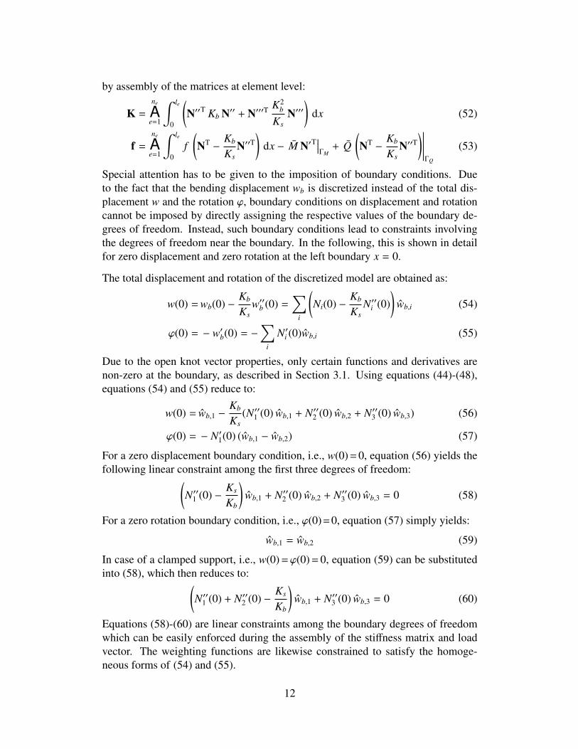
4. Numerical tests

In this section, we study several examples to investigate various aspects of the pre-sented methods. First, we test the imposition of different boundary conditions. Af-ter that, we study convergence behavior. Finally, we perform a shear-locking studyvarying the beam slenderness, and compare the results to those of standard Timo-shenko and Bernoulli-Euler beam formulations.

0 0.2 0.4 0.6 0.8 1

0

0.02

0.04

0.06

0.08

0.1

0.12

0.14

0.16

w

x

(a)

0 0.2 0.4 0.6 0.8 1

0

0.005

0.01

0.015

0.02

0.025

0.03

0.035

w

x

(b)

0 0.2 0.4 0.6 0.8 1

0

0.2

0.4

0.6

0.8

1

1.2

1.4

1.6

w

x

(c)

0 0.2 0.4 0.6 0.8 1

−0.2

−0.1

0

0.1

0.2

0.3

0.4

0.5

0.6

w

x

(d)

Figure 4: Beam with constant load and different boundary conditions. Displacement plots for thefollowing cases: (a) simply supported; (b) clamped; (c) left end clamped, right end free (cantilever);(d) left end simply supported with boundary moment Ml, right end with zero-rotation slider supportand a boundary force Qr. The dashed lines show the undeformed beam

4.1. Beam with uniform load and different boundary conditions

To test the imposition of different boundary conditions, we consider the followingcases:

(a) simply supported;

14

(b) clamped;

(c) left end clamped, right end free (cantilever);

(d) left end simply supported with boundary moment Ml, right end with zero-rotation slider support and a boundary force Qr;

Assuming the parameters f = Qr = Ml = l = 1 the analytical solution for the totaldisplacement w is given for the four cases as follows:

(a) w(x) = 124 Kb

(x4 − 2x3 + x

)+ 1

2 Ks

(−x2 + x

)(b) w(x) = 1

24 Kb

(x4 − 2x3 + x2

)+ 1

2 Ks

(−x2 + x

)(c) w(x) = 1

24 Kb

(x4 − 4x3 + 6x2

)+ 1

2 Ks

(−x2 + 2x

)(d) w(x) = 1

24 Kb

(x4 − 8x3 + 12x2 − 4x

)+ 1

2 Ks

(−x2 + 4x

)Since f is constant, the analytical solution is of fourth order in all cases. Therefore,we model the beam by one quartic element, which should be capable of representingthe solution exactly, using the Galerkin formulation and applying the boundary con-ditions as described in Section 3.2. For the collocation formulation, strictly speak-ing, quintic basis functions are necessary since this is the minimum polynomialdegree for which the fourth derivatives are continuous and thus for computing theGreville abscissae corresponding to the fourth derivative space, see (62). However,we can develop a successful formulation for quartic basis functions too, if standardGreville abscissae are used. This is the analog of what has been done in the secondorder case, for which quadratic basis functions have been shown effective [4].

For the computations, we consider a beam with a rectangular cross-section and thefollowing geometrical and material parameters: width 0.1, thickness 0.01, Young’smodulus 107, Poisson’s ratio 0.2 and a shear correction factor of 5/6. Figure 4shows the displacement results for the four cases, which are obtained by both theGalerkin and collocation methods and exactly represent the analytical solutions re-ported above.

4.2. Convergence studies

We apply a sinusoidal load function f (x) = 16 π4 cos(2πx) and consider a clampedboundary condition on the left end and a slider support on the right end. The prob-lem setup is shown in Figure 5, the beam length is l=1. The analytical solution forthe total displacement is given by:

w(x) =1

Kb(cos(2πx) − 1) +

1Ks

(4π2 cos(2πx) − 4π2

)(68)

15

f(x) = 16⇡4 cos(2⇡x)

Figure 5: Beam with sinusoidal load, clamped left and slider support right.

From equation (68), the analytical solution for the variables ϕ, M, and Q can easilybe derived. A rectangular cross-section is considered with the same geometricaland material parameters as in the previous case, with the exception of the beamthickness, for which two cases are considered, a thin beam (t = 10−4) and a thickbeam (t = 10−1). We perform refinement studies for different polynomial degreesand evaluate the error in the L2-norms for the total displacement w, the rotation ϕ,the bending moment M, and the shear force Q.

For the Galerkin formulation, polynomial degrees p = 3, 4, 5 are used. The resultsfor the thin beam are depicted in Figure 6, those for the thick beam in Figure 7. Itcan be observed that in the case of the thin beam, the convergence rates are, at least,p + 1 for w, p for ϕ, p − 1 for M, and p − 2 for Q. These are the same convergencerates as obtained by the corresponding Bernoulli-Euler beam formulation (with theBernoulli-Euler solution as reference solution).

This example is also solved by the proposed isogeometric collocation approach.In this case, polynomial degrees p = 5, 6, 7 are used. Figure 8 shows the resultsobtained with collocation for the thin beam and Figure 9 for the thick beam. As canbe seen, the errors of all variables are practically identical for the thin and the thickcase, with convergence rates of, at least, p − 2 for even and p − 3 for odd degrees.The same behavior has been observed for collocation methods of Bernoulli-Eulerbeams [17].

4.3. Locking study and comparison with standard Timoshenko and Bernoulli-Eulerbeam formulations

In this section, we perform a locking study by varying the slenderness, defined aslength over thickness l/t, keeping the polynomial degree and the number of degreesof freedom fixed. Moreover, we compare the results obtained with the new Galerkinformulation to those obtained by “standard” Timoshenko and Bernoulli-Euler beamformulations. In the “standard” Timoshenko formulation displacement and rotationare discretized independently with equal order approximations. Clearly, such a for-mulation has more degrees of freedom for the same number of elements. For a fair

16

1.2 1.4 1.6 1.8−11

−10

−9

−8

−7

−6

−5

−4

−3

log10(#dof)

log 10

( ||w

ex −

wh|| L2 /

||w

ex|| L2 )

p=3p=4p=5c1*(#dof)−4

c2*(#dof)−5

c3*(#dof)−6

(a)

1.2 1.4 1.6 1.8−9

−8

−7

−6

−5

−4

−3

−2

log10(#dof)

log 10

( ||q

ex −q h|| L2 /

||q ex

|| L2 )

p=3p=4p=5c1*(#dof)−3

c2*(#dof)−4

c3*(#dof)−5

(b)

1.2 1.4 1.6 1.8−8

−7

−6

−5

−4

−3

−2

−1

log10(#dof)

log 10

( ||M

ex −

Mh|| L2 /

||M

ex|| L2 )

p=3p=4p=5c1*(#dof)−2

c2*(#dof)−3

c3*(#dof)−4

(c)

1.2 1.4 1.6 1.8−5.5

−5

−4.5

−4

−3.5

−3

−2.5

−2

−1.5

−1

−0.5

log10(#dof)

log 10

( ||Q

ex −

Qh|| L2 /

||Q

ex|| L2 )

p=3p=4p=5c1*(#dof)−1

c2*(#dof)−2

c3*(#dof)−3

(d)

Figure 6: Convergence studies for a thin beam, t=10−4, solved with the Galerkin formulation. Errorin the L2-norm for (a) total displacement w, (b) rotation ϕ, (c) bending moment M, and (d) shearforce Q.

comparison, all methods use B-splines basis functions with the same polynomial de-gree and the same number of degrees of freedom. We consider a simply supportedbeam with the sinusoidal load described in Section 4.2. The beam is discretizedwith cubic B-splines and there are 16 degrees of freedom. Different slendernessratios, ranging from 5 up to 10, 000, are considered.

Figure 10 shows the normalized strain energy as a function of the slenderness for thedifferent formulations. It can be seen that the Timoshenko formulation with stan-dard discretization exhibits initial locking for a slenderness of 50, which dramati-cally increases for slenderness values higher than 100. It should also be noted thatdue to the higher polynomial degree employed here, the locking effects are less pro-nounced than for a standard linear Timoshenko finite element. The Bernoulli-Eulerbeam, on the other hand, yields correct results in the thin regime but underestimatesthe strain energy for slenderness values lower than 50, for which the shear defor-mation is not negligible. As can be seen, the presented single-variable Timoshenkoformulation yields good results for the entire range of slenderness considered.

17

1.2 1.4 1.6 1.8−9

−8

−7

−6

−5

−4

−3

−2

log10(#dof)

log 10

( ||w

ex −

wh|| L2 /

||w

ex|| L2 )

p=3p=4p=5c1*(#dof)−2

c2*(#dof)−3

c3*(#dof)−4

(a)

1.2 1.4 1.6 1.8−9

−8

−7

−6

−5

−4

−3

−2

log10(#dof)

log 10

( ||q

ex −q h|| L2 /

||q ex

|| L2 )

p=3p=4p=5c1*(#dof)−2

c2*(#dof)−4

c3*(#dof)−5

(b)

1.2 1.4 1.6 1.8−8

−7

−6

−5

−4

−3

−2

−1

log10(#dof)

log 10

( ||M

ex −

Mh|| L2 /

||M

ex|| L2 )

p=3p=4p=5c1*(#dof)−2

c2*(#dof)−3

c3*(#dof)−4

(c)

1.2 1.4 1.6 1.8−5.5

−5

−4.5

−4

−3.5

−3

−2.5

−2

−1.5

−1

−0.5

log10(#dof)

log 10

( ||Q

ex −

Qh|| L2 /

||Q

ex|| L2 )

p=3p=4p=5c1*(#dof)−1

c2*(#dof)−2

c3*(#dof)−3

(d)

Figure 7: Convergence studies for a thick beam, t = 10−1, solved with the Galerkin formulation.Error in the L2-norm for (a) total displacement w, (b) rotation ϕ, (c) bending moment M, and (d)shear force Q.

18

1.2 1.4 1.6 1.8−8

−7

−6

−5

−4

−3

−2

−1

log10(#dof)

log 10

( ||w

ex −

wh|| L2 /

||w

ex|| L2 )

p=5p=6p=7c1*(#cp)−2

c2*(#cp)−4

(a)

1.2 1.4 1.6 1.8−8

−7

−6

−5

−4

−3

−2

−1

log10(#dof)

log 10

( ||q

ex −q h|| L2 /

||q ex

|| L2 )

p=5p=6p=7c1*(#cp)−2

c2*(#cp)−4

(b)

1.2 1.4 1.6 1.8−8

−7

−6

−5

−4

−3

−2

−1

log10(#dof)

log 10

( ||M

ex −

Mh|| L2 /

||M

ex|| L2 )

p=5p=6p=7c1*(#cp)−2

c2*(#cp)−4

(c)

1.2 1.4 1.6 1.8−8

−7

−6

−5

−4

−3

−2

−1

log10(#dof)

log 10

( ||Q

ex −

Qh|| L2 /

||Q

ex|| L2 )

p=5p=6p=7c1*(#cp)−2

c2*(#cp)−4

(d)

Figure 8: Convergence studies for a thin beam, t = 10−4, solved with the collocation formulation.Error in the L2-norm for (a) total displacement w, (b) rotation ϕ, (c) bending moment M, and (d)shear force Q.

19

1.2 1.4 1.6 1.8−8

−7

−6

−5

−4

−3

−2

−1

log10(#dof)

log 10

( ||w

ex −

wh|| L2 /

||w

ex|| L2 )

p=5p=6p=7c1*(#cp)−2

c2*(#cp)−4

(a)

1.2 1.4 1.6 1.8−8

−7

−6

−5

−4

−3

−2

−1

log10(#dof)

log 10

( ||q

ex −q h|| L2 /

||q ex

|| L2 )

p=5p=6p=7c1*(#cp)−2

c2*(#cp)−4

(b)

1.2 1.4 1.6 1.8−8

−7

−6

−5

−4

−3

−2

−1

log10(#dof)

log 10

( ||M

ex −

Mh|| L2 /

||M

ex|| L2 )

p=5p=6p=7c1*(#cp)−2

c2*(#cp)−4

(c)

1.2 1.4 1.6 1.8−8

−7

−6

−5

−4

−3

−2

−1

log10(#dof)

log 10

( ||Q

ex −

Qh|| L2 /

||Q

ex|| L2 )

p=5p=6p=7c1*(#cp)−2

c2*(#cp)−4

(d)

Figure 9: Convergence studies for a thick beam, t = 10−1, solved with the collocation formulation.Error in the L2-norm for (a) total displacement w, (b) rotation ϕ, (c) bending moment M, and (d)shear force Q.

20

100 101 102 103 1040

0.2

0.4

0.6

0.8

1

slenderness l/t

norm

aliz

ed s

train

ene

rgy

BernoulliTimoshenko standardTimoshenko single−variable

Figure 10: Locking study and comparison of the present single-variable formulation with standardTimoshenko and Bernoulli-Euler beam formulations: normalized strain energy as a function of theslenderness. Cubic B-splines are used for all formulations, “standard” Timoshenko indicates that wand ϕ are discretized independently with equal order approximation.

21

5. Conclusions

We have presented single-variable formulations for the Timoshenko beam problemwith the bending displacement as the only unknown variable. The strong form dif-ferential equation is of fourth order, while the symmetric weak form is of third order.We use B-Splines of suitable continuity for discretization, and establish isogeomet-ric Galerkin and collocation approaches based on the weak and the strong form,respectively. Since there is only one variable, these formulations involve only halfof the degrees of freedom compared to standard Timoshenko formulations. At thesame time shear locking is precluded ab initio. Several numerical examples demon-strate the validity and efficiency of the presented methods. In future research, wehope to extend this approach to shear-deformable plates and shells.

6. Acknowledgement

T.J.R. Hughes was supported by grants from the Office of Naval Research (N00014-08-1-0992), the National Science Foundation (CMMI-01101007), and SINTEF (UTA10-000374) with the University of Texas at Austin.

J. Kiendl, A. Reali, and F. Auricchio were partially supported by the EuropeanResearch Council through the FP7 Ideas Starting Grant n. 259229 ISOBIO. Thissupport is gratefully acknowledged.

References

[1] F. Auricchio, L. Beirao da Veiga, T.J.R. Hughes, A. Reali, and G. Sangalli.Isogeometric collocation methods. Mathematical Models and Methods in Ap-plied Sciences, 20(11):2075–2107, 2010.

[2] F. Auricchio, L. Beirao da Veiga, T.J.R. Hughes, A. Reali, and G. Sangalli.Isogeometric collocation for elastostatics and explicit dynamics. ComputerMethods in Applied Mechanics and Engineering, 249-252:2–14, 2012.

[3] F. Auricchio, L. Beirao da Veiga, J. Kiendl, C. Lovadina, and A. Reali.Locking-free isogeometric collocation methods for spatial Timoshenko rods.Computer Methods in Applied Mechanics and Engineering, 263:113–126,2013.

[4] L. Beirao da Veiga, C. Lovadina, and A. Reali. Avoiding shear locking for theTimoshenko beam problem via isogeometric collocation methods. ComputerMethods in Applied Mechanics and Engineering, 241-244:38–51, 2012.

[5] J.A. Cottrell, T.J.R. Hughes, and Y. Bazilevs. Isogeometric Analysis: TowardIntegration of CAD and FEA. Wiley, 2009.

22

[6] J.A. Cottrell, A. Reali, Y. Bazilevs, and T.J.R. Hughes. Isogeometric anal-ysis of structural vibrations. Computer Methods in Applied Mechanics andEngineering, 195:5257–5296, 2006.

[7] L. De Lorenzis, J.A. Evans, T.J.R. Hughes, and A. Reali. Isogeometric col-location: Neumann boundary conditions and contact. ICES Report, 14-06,2014.

[8] G. Falsone and D. Settineri. An Euler-Bernoulli-like finite element method forTimoshenko beams. Mechanics Research Communications, 38:12–16, 2011.

[9] H. Gomez, A. Reali, and G. Sangalli. Accurate, efficient, and(iso)geometrically flexible collocation methods for phase-field models. Jour-nal for Computational Physics, 262:153–171, 2014.

[10] L. Greco and M. Cuomo. B-Spline interpolation of Kirchhoff-Love spacerods. Computer Methods in Applied Mechanics and Engineering, 256:251–269, 2013.

[11] T.J.R. Hughes. The Finite Element Method, Linear Static and Dynamic FiniteElement Analysis. Dover Publications Inc., 2000.

[12] T.J.R. Hughes, J.A. Cottrell, and Y. Bazilevs. Isogeometric analysis: CAD,finite elements, NURBS, exact geometry, and mesh refinement. ComputerMethods in Applied Mechanics and Engineering, 194:4135–4195, 2005.

[13] K. Kapur. Vibrations of a Timoshenko beam using finite-element approach.Journal of the Acoustic Society of America, 40:1058–1063, 1966.

[14] J. Kiendl, F. Auricchio, L. Beirao da Veiga, C. Lovadina, and A. Reali. Isogeo-metric collocation methods for the Reissner-Mindlin plate problem. submittedto Computer Methods in Applied Mechanics and Engineering, 2014.

[15] J. Kiendl, K.-U. Bletzinger, J. Linhard, and R. Wuchner. Isogeometric shellanalysis with Kirchhoff-Love elements. Computer Methods in Applied Me-chanics and Engineering, 198:3902–3914, 2009.

[16] X.-F. Li. A unified approach for analyzing static and dynamic behaviors offunctionally graded Timoshenko and Euler-Bernoulli beams. Journal of Soundand Vibration, 318:1210–1229, 2008.

[17] A. Reali and H. Gomez. An isogeometric collocation approach for Bernoulli-Euler beams and Kirchhoff plates. In preparation, 2014.

[18] D. Schillinger, J.A. Evans, A. Reali, M.A. Scott, and T.J.R. Hughes. Isogeo-metric collocation: Cost comparison with Galerkin methods and extension toadaptive hierarchical NURBS discretizations. Computer Methods in AppliedMechanics and Engineering, 267:170–232, 2013.

23