ICES CM 2005/L:21 The spatial dimension of ecosystem structure and dynamics

Using geostatistics to quantify annual distribution and aggregation patterns of fishes in the

Eastern English Channel.

S. Vaz, C. S. Martin, B. Ernande, F. Coppin, S. Harrop and A. Carpentier.

The Eastern English Channel is an area with strong hydrodynamic features supporting, among

other human activities, an important fishery exploitation. Since 1988, IFREMER (French

Research Institute for Exploitation of the Sea) has been carrying out an essential ground fish

survey primarily dedicated to ICES annual assessment of major commercial fish stocks in this

area. However, these fisheries independent data also offer the opportunity to study of the

distribution patterns of observed fish species using geostatistical techniques. Geostatistics

embody a suite of methods for analysing spatial data and allow the estimation of the values of

a variable of interest at non sampled locations from more or less sparse sample data points.

Geostatistical estimation (kriging) is different from other interpolation methods because it

uses a model describing the spatial structure and variation in the data – the variogram. The

latter is the central tool of geostatistics and is essential for all of the other geostatistical

methods. Kriging was used to produce distribution maps of several fish species over 17 years

(1988-2004) and variogram parameters reflected changes in distribution patterns over time.

Fish aggregation patterns and inter-annual variability were examined in the light of

geostatistical analyses of fish distribution and a few example of this study will be presented.

Key-words: Eastern English Channel, CHARM, Fish spatial distribution patterns, geostatistics

Contact author:

S. Vaz: Ifremer, Laboratoire Ressources Halieutiques, 150 quai Gambetta, BP699, 62321,

Boulogne/mer, France [tel: (+33) 3 21 99 56 00, fax: (+33) 3 21 99 56 01, e-mail:

svaz@ifremer.fr

S. Vaz, F. Coppin and A. Carpentier: Ifremer, Laboratoire Ressources Halieutiques, 150 quai

Gambetta, BP699, 62321, Boulogne/mer, France [tel: (+33) 3 21 99 56 00, fax: (+33) 3 21

99 56 01, e-mail: svaz@ifremer.fr]. B. Ernande: Ifremer, Laboratoire Ressources

Halieutiques, avenue du Général de Gaulle, 14520 Port-en-Bessin, France [tel: (+33) 2 31

51 56 00, fax: (+33) 2 31 51 56 01, e-mail: Bruno.Ernande@ifremer.fr]. C. S. Martin:

Department of Geographical and Life Sciences, Canterbury Christ Church University,

Canterbury CT1 1QU, U. K. [tel: (+44) 1227 767700 (ext. 2324), e-mail:

c.s.martin@canterbury.ac.uk].

INTRODUCTION

The analysis of spatial patterns is of prime importance since most natural phenomena are

affected by processes that have spatial components generating spatially recognisable

structures, such as patches or gradients, which can be analysed. Ecological data may include

several types of spatial patterns occurring at different scale such as trends at larger scale,

patchiness at intermediate and local scales and random fluctuation or noise at smaller scale

(Fortin and Dale, 2005).

Species distribution results from the combined action of several forces, some of which are

external (environmental), whereas others are intrinsic to the community (Legendre and

Legendre, 1998). Community structure and environmental attributes, result from many

physical and biological processes that interact, some in non-linear or chaotic ways. The

outcome is so complex that the variation over a region, of almost any size, appears to be

random (Webster and Oliver, 2001). This requires the probabilistic approach, which

underpins geostatitics. The randomness, which is embodied in the random function model on

which geostatistics are based, is not a property of the physical world (Webster and Oliver,

1990). In reality, ecosystem spatial heterogeneity is deterministic and is not the result of some

random, noise-generating process (Legendre and Legendre, 1998).

Originally developed for the mining industry, geostatistics were first developed to address

specific needs of spatial prediction of geological resources over two or three dimensional

areas. This last feature made the technique known rapidly in oceanography (Fortin and Dale,

2005) but it took longer to become widespread in ecology (Rossi et al., 1992) and longer still

to find its way to marine ecology. Many demersal and benthic fishes exhibit particular

distribution and aggregation patterns at annual time scale in association with particular

habitats or phases of their life cycle (Mello and Rose, 2005). Although there is a limited

understanding about how geostatistics may be used for such end, they are particularly suited

for fishes exhibiting gregarious behaviour but seasonally variable distributions. Spatial

structures, in particular that of fish distribution, can be identified and described quantitatively

using geostatistics (Petitgas, 1993 and 2001, Mello and Rose, 2005) .

This study investigated the use of geostatistical methods to quantify annual distribution

patterns over a broad range of species obtained from scientific survey. An overview of

geostatistical concepts and result interpretation is presented here with little detail about the

statistical computation involved. A simple methodology enabling geostatistical analyses and

kriging interpolation for cartography and suiting many species data, over a large range of

years and originating from the same survey, is proposed. The results are discussed in relation

to season, habitat, and migration patterns.

METHODS

Survey design and data collection

IFREMER contributes to the acquisition of basic biological data through its annual

experimental trawling survey called CGFS (Channel Ground Fish Survey). The CGFS has

been carried out each year since 1988 on-board the research vessel Gwen Drez in October.

The survey extends from the Eastern English Channel to the south of the North Sea, which

corresponds to ICES divisions VIId and IVc. The study area is divided into rectangles of 15'

latitude and 15' longitude using a systematic sampling strategy. The sampling gear is a high

opening bottom trawl well adapted for catching demersal species, with a 10 mm mesh size

(side knot) for catching juveniles. This sampling gear is polyvalent and is well adapted to the

varying seabed types encountered in the study area. One or two 30 minutes hauls are

performed within each rectangle of the CGFS grid. The fishing hauls are chosen using

professional fishing plans or found by prospecting. The fishing method is standardised:

sampling stations are each year at similar locations each year and identical sampling gear is

used. At each sampling station, all the fish species are sorted, weighed, counted and

measured. Data available for the period 1988 to 2004 were used to compute variograms and

map species distribution (Fig.1).

Statistical analyses Statistics and methods in ecology require the careful examination of the data distribution,

because ecological variables (descriptors) are assumed not to have a uniform scale. Although

most of the methods do not require full normality, they perform better if the distribution is as

near to normal as possible. Moreover, the statistical distribution of the data must be examined

to determine whether the assumptions upon which geostatistics are based hold (Rossi et al.,

1992). The statistical distribution of environmental or biological data were tested for

normality using histograms, skewness and kurtosis. The data were transformed when

skewness value exceeded |1| and/or kurtosis exceeded 1 and when a normalising function that

could improve the data distribution was found. Biological variables were measured on scales

based on analytical conventions and they are unrelated to the natural processes that generate

them. Therefore, any transformed scale is as appropriate as those on which these data were

originally recorded (Legendre and Legendre, 1998). Species abundance were expressed as

density values (nbr.km-2) and always required to be log-transformed using log10(x+1)

transformation (where x is the species abundance value).

Geostatistics

Geostatistical methods were developed for spatially structured mining data during the 1960s

(Matheron, 1965) and embody a suite of methods for analysing spatial data and allow the

estimation of the values of a variable of interest at non sampled locations from more or less

sparse sample data points.

The variogram

The variogram, the central tool of geostatistics, is a function that measures the relation

between pairs of observations a certain distance apart. It summarises the way in which the

variance of a variable changes as the distance and direction separating any two points varies.

Typically, for spatially structured data, the variance is small at short lags and increase with

larger separating distance (monotonic increasing) (Fig.2). The variogram may increase to a

maximum at which it remains thereafter. This upper bound, the sill variance, estimates the

maximum variance of the data and indicates that the variances between points are no longer

correlated. The lag distance at which the sill is reached (the range) marks the limit of spatial

dependence i.e. it describes the extent of the observed pattern. The range size is related to the

spatial continuity of the variable of interest and a variable with long-range is more spatially

continuous than a short range one. The variogram often has a positive intercept on the

ordinate known as the nugget variance. The nugget is the amount of variance not explained

by the spatial model. This arises from a combination of error terms attributable to

inappropriate sampling, measurement or analytical errors and random variation, but mostly

from variation occurring over distances smaller that the sampling interval.

Modelling the variogram

Many variograms have simple forms that can be described by a limited set of authorised

models (Fig.3a-e). These models must be capable of describing the main features of the

variogram, i.e. the nugget, the shape of the monotonic increase and the sill. The most common

way of fitting models is by the statistical procedure of least squares approximation. The

chosen model should be the one with the best statistical and visual fit. The parameters of the

model estimate the nugget and the sill variances, and the distance parameter. From the latter,

the scale of variation of a particular variable can be determined, compared with that of others

and can be used to determine the limit of spatial dependence of this variable.

Circular, spherical and pentaspherical models curve (in increasing order of gradation) more

gradually than boundedlinear models. All of them represents transition features that have a

common extent and appear as patches, some with large values some with small ones. The

range (r) of the model is the average diameter (D) of the patches (Webster and Oliver, 2001).

Exponential function approaches its sill asymptotically and does not have a finite range. The

average diameter (D) of the patches can be approximated as 3r, which is the distance at which

the variogram has reached 95% of its sill. Variograms fitted by this model illustrate a

transition process in which the structures have random extents. Such a variogram should be

expected where differences in abundance level are the main contributors to abundance

variation and where boundaries between levels occur at random (Webster and Oliver, 2001).

Some variograms appear completely flat, i.e. “pure nugget”, meaning that there is no spatial

dependence evident in the data (Fig. 3f).

Measure of the spatial structuration

The level of spatial structure can be inferred from the ratio, Q, given by:

Q = C / (C+C0)

Where C+C0 is the sill and C0 is the nugget variance; hence C is the variance

attributable to spatial dependence. The ratio Q varies between 0 and 1: a ratio of 0 indicates

the absence of spatial structure at the sampling and support scale used; as Q approaches 1, a

greater proportion of the variability is explained by the variogram model.

Kriging interpolation

The method of prediction embodied in geostatistics and for which the variogram parameters

are essential, is known as “kriging”. Kriging produces optimal unbiaised estimates that can be

used for mapping by taking into account the way that a variable varies in space to predict the

values at unsampled locations. It is a method of weighted averaging based on the variogram

model of the spatial variation. Finally, estimation variance is known and is the minimum,

whereas classical methods are based on arbitrary mathematical functions and provide no

measure of error variances. Ordinary kriging is the most commonly used method. It can be

used to produce a large field of estimates at points or blocks and corresponding variances for

mapping. The weights are obtained from the variogram model and are derived as to minimize

the estimation variance. Generally, the weights of points near the point to be kriged are large

and these decrease as the distance increases. The nearest four or five might contribute 80% of

the total weight and the nearest 10 almost all the remainder. Similarly, clustered points carry

less weight individually than isolated ones at the same distance. Finally, some data points may

be screened by points lying between them and the point to be kriged. These effects are

desirable and show that kriging is local. Block kriging, producing average estimate value

within a prescribed area rather than punctual location, was preferred. Block size matched that

of interpolation grid so that the grid nods corresponded to the block centre and blocks did not

overlap.

Spatial trend or drift

Local trend or drift violates the assumption of the random function model, because the values

change in a smooth predictable way, they are deterministic and are no longer random (Isaaks

and Srivaslastava, 1989). In this case, the variogram would have a concave upward form.

Variables must be examined for trend at the outset by fitting a low-order polynomial (linear or

quadratic regression) on the spatial coordinates (Webster and Oliver, 2001). Linear function

for two dimentional trends corresponds to an inclined plane (such as a drift in depth value

from inshore to offshore) whilst quadratic function correspond to a curved surface simulating

an edge effect (such as depth value around an island or in an enclosed bay or strait surrounded

by coastlines). When the fitted function accounts for over 20 % of the variance, a variogram

should be computed using the residuals and compared to the variogram of the original data.

When the presence of a gradual trend in the data is confirmed, universal kriging, an adaptation

of ordinary kriging, allows one to accommodate such trend. Universal kriging was used to

produce good local estimate in the presence of a trend and like ordinary kriging the procedure

was automatic once a satisfactory function for the variogram was found.

The kriged estimates can be used to map the variable of interest in order to interpret the

spatial pattern described by the variograms. In the present study, the spatial variation of

biological and environmental data were analysed using Genstat (Genstat 7 Committee, 2004),

which is a GENeral STATistics package that includes the main geostatistical tools. It

computes experimental variograms, fits these with various authorised mathematical models

and uses them to calculate kriged estimates on a fine regular grid of 0.1 decimal degree mesh

size.

Survey resolution and kriging search parameters

Prior any species analyses could take place, a preliminary data exploration resulted in

optimised search parameters to suit the survey design across all years and were set constant

for all kriging procedures. First the longitude coordinates were corrected so that longitude

decimal degree were set to be the same metric distance as the latitude decimal degree. This is

done by the following projection transformation:

Corrected longitude = longitude * cos((latitude*pi)/180)

After geostatistical analyses and kriging interpolation have taken place, longitude was back-

transformed to enable mapping with true coordinates. The average distance between close

pair of observations, corresponding to the survey resolution, was 0.1° and was used to set the

kriging grid mesh size. Search radius was set to 0.2 (twice the grid mesh size) and number of

neighbours used for kriging were taken between a set minimum of 4 and maximum of 7 data

points.

Mapping

Using ArcMap’s Spatial Analyst extension, the grid of data points was then interpolated by

kriging, using the default parameters of the software (ordinary kriging, spherical variogram

model, variable search radius with 12 points) to create a continuous raster of 1 km2 cell size

(resolution). ArcMap’s Raster Calculator extension was then used to cut out any portion of the

raster that was “extrapolated”, i.e. that was outside of the geographical area covered by the

original data point grid. When the area surveyed varied across years, the resulting maps differ

in geographical extent.

Geostatistical analyses and kriging were used extensively to analyse the spatial structure of

sixteen fish species over 17 years (1988-2004). Their variogram parameters that reflected the

changes in their distribution patterns over time were defined and the resulting maps illustrate

the spatial distributions and their variation over time of the species in the Eastern English

Channel.

RESULTS

Three species will be presented in this study as example of result and interpretation. These

were Microstomus kitt (lemon sole), Raja clavata (thornback ray), Scyliorhinus canicula

(lesser-spotted dogfish). Experimental variograms were computed and fitted with

authorised models using Genstat software (Fig 3a-f).

Microstomus kitt (lemon sole)

The geostatistical results for this species are presented in Table 1 and illustrate the case of a

relatively strongly spatially structured distribution (Q = 0.69 corresponding to 69% of the data

variability being explained by the variogram model in average over 17 years). The average

diameter (D) of the observed patches was 0.7° over the entire period but varied greatly from

year to year (from 0.3° up to 1.6°). Various type of models were used indicating that some

years the patch sizes were relatively constant (boundedlinear, circular, pentaspherical) and

some others spatial structures had random extent (exponential models). Often years with

spatial distribution displaying large patch size (D>0.7) were modelled with an exponential

model illustrating their random extent. Trends sometimes occurred (1990, 1994-96, 2004) and

corresponded to years with relatively small range (D<0.6) illustrating the almost exclusively

north-eastern distribution of this species for these years (Fig. 4). This species generally occurs

on gravely seabeds mostly in the Dover strait and sometimes in the centre of the Eastern

English Channel where tidal flows are at their greatest.

Raja clavata (thornback ray)

The geostatistical results for this species are presented in Table 2 and illustrate the case of a

species with a relatively small average diameter (D) of the observed patches (0.56° over the

entire period). It was not as strongly structured as lemon sole (average Q = 0.56). Models

indicating that patch sizes were relatively constant within a particular year (boundedlinear,

circular, spherical, pentaspherical) were predominent however the average path extent varied

greatly from year to year (0.1° up to 1.2°). Trend effect never occurred illustrating the patchy

distribution of this species with no direct relation to coastal proximity or geographic

preferences within the area of study (Fig. 5). Maps illustrate their preferences for central

Eastern English Channel but also highlight how this species may be found more inshore some

years along both French and English coasts, near mouths of estuaries and in sandy bays along

southern English Coast.

Scyliorhinus canicula (lesser-spotted dogfish)

The geostatistical results for this species are presented in Table 3 and illustrate the case of a

species with a relatively large average diameter (D) of the observed patches (1.04° over the

entire period) that did not vary greatly from year to year (from 0.7° up to 1.4°). The model

used indicated that the patch sizes were relatively constant within each years (boundedlinear,

circular, spherical, pentaspherical). This species was not has spatially structure as the two

previous ones (average Q = O.47) due to three isolated years (1989, 1993, 2002) where no

spatial structure could be found. These years also corresponded to the only times significant

quadratic trends could be detected meaning that long-range drift was the only spatial structure

that can be found in the data in these instances. This species displayed a relatively broad

distribution across the central region of the Eastern English Channel that sometime extended

in the Dover Strait (Fig 6).

DISCUSSION

The distribution maps reflected the species habitat preferences in this area of the English

Channel. Lemon sole is a benthic species living on gravels or shelly sand between 40 and 200

m depth. In the Eastern English Channel its distribution is almost exclusively limited to the

Dover Strait where hard seabed sediment and strong tidal current are found. Patch of variable

extent and trend in their distribution for high abundance in this area could be quantified and

identified through the geostatistical analyses process. Moreover, this study revealed that this

species was strongly structured in space highlighting its strong affinity to a particular habitat

in this area. Thornback ray is a demersal species preferring hard and sandy bottoms of the

continental slope and illustrated by its patchy and variable distribution in the area. Thornback

ray was relatively well structured but although its affinity for hard sediment type was

confirmed by its yearly distribution, it had no affinity for any particular area in the Eastern

English Channel and its localisation and extent changed from year to year probably in relation

to its total abundance. Geostatistical analyses enabled the quantification of this distribution

and revealed that the patch extent where relatively small. Lesser-spotted dogfish is a bentho-

demersal species that inhabits gravel and sandy bottoms on the continental shelves. Its

distribution extended largely in the deepest areas of the Eastern English Channel over large

area of hard seabed sediments. Geostatistical results revealed the large extent of the observed

patterns in this species distribution but also its relatively small spatial structuration. This

result raise question about the survey resolution and design and its effectiveness to capture

efficiently the true spatial heterogeneity of this species that may occur on a smaller scale than

the one that could be observed.

CONCLUSION AND PERSPECTIVE

Many interpolation techniques may be used for illustration purpose. However, geostatistics

enable to explore, characterise and quantify spatial structure as well as interpolation (Fortin

and Dale, 2005) and should be preferred to other techniques. In the process of studying the

variogram structure and modelling it for accurate interpolation, valuable information about

the spatial process taking place is obtained. Measure of patch size, global trends and spatial

structuration are made and can be used to support the description of the species distribution

patterns in relation to their habitat preferences and spatial behaviour. Moreover, generic and

relatively simple methods and softwares now enable its use and bring geostatistics to novice

reach without loosing its accuracy and risking the “black-box” approach often proposed in

GIS software. In the framework of an international project (CHARM project,

http://charm.canterbury.ac.uk), 16 fish species spatial distribution could be analysed and

mapped based on 16 years data and two seasons (Carpentier et al., 2005) in a relatively short

time span proving that geostatistics could be efficiently used for large scale studies aimed at

ecosystemic understanding of marine living resources.

Further to geostatistical analyses, other spatial analyses may be used to quantify the

aggregation patterns of fish (see Fortin and Dale, 2005 for full review). However, some

techniques such as geostatistical aggregation curves (Petitgas, 1998) may give useful insight

about how the spatial distribution changes as the population abundance varies linking fish

distribution to density-dependent population dynamics. Based on these aggregation curves,

patch gravity centre and boundaries may be defined and compared across years to further

characterise the link between the population demography and its spatial distribution

behaviour.

ACKNOWLEDGEMENTS

This study was realised within the framework of the French-English INTERREG IIIA Eastern

Channel Habitat Atlas for Marine Resource Management with the financial support of

European Fundings managed by the Haute-Normandie Region.

REFERENCES

Carpentier, A., Vaz, S., Martin, C. S., Coppin, F., Dauvin, J. –C., Desroy, N., Dewarumez, J.–

M., Eastwood, P. D., Ernande, B., Harrop, S., Kemp, Z., Koubbi, P., Leader-Williams, N.,

Lefèbvre, A., Lemoine, M., Meaden, G. J., Ryan, N., Walkey, M., 2005. Eastern Channel

Habitat Atlas for Marine Resource Management (CHARM), Atlas des Habitats des

Ressources Marines de la Manche Orientale, INTERREG IIIA.

Fortin, M-J and Dale, M, 2005. Spatial Analysis: A guide for Ecologists. Cambridge

University Press.

GenStat Release 7.1 Copyright 2004, Lawes Agricultural Trust (Rothamsted Experimental

Station). R.W. Payne, S.A. Harding, D.A. Murray, D.M. Soutar, D.B. Baird, S.J. Welham,

A.F. Kane, A.R. Gilmour, R. Thompson, R. Webster, G. Tunnicliffe Wilson. Published by

VSN International, Wilkinson House, Jordan Hill Road, Oxford, UK.

Isaaks, EH and Srivastava, RM, 1989. An introduction to applied geostatistics. Oxford

University Press.

Legendre P & Legendre L, 1998. Numerical Ecology. Elsevier, Amsterdam.

Matheron G, 1965. Les variables regionalisées et leur estimation. Masson, ed. Paris.

Mello LGS and Rose GA (2005). Using geostatistics to quantify seasonal distribution and

aggregation patterns of fishes: an example of Atlantic Cod (Gadus morhua). Can. J. Fish.

Aquat. Sci. 62:659-670.

Petitgas, P, 1993. Geostatistics for fish stock assessment : a review and acoustic application.

ICES J. Mar. Sci. 50 :285-298.

Petitgas, P, 1998. Biomass-dependent dynamics of fish spatial distributions characterised by

geostatistical aggregations curves. ICES J. Mar. Sci. 55 : 147-153

Petitgas, P, 2001. Geostatistics in fisheries survey design and stock assessment: models,

variances and applications. Fish and Fisheries 2: 231-249.

Rossi RE, Mulla DJ, Journel, AG & Franz EH, 1992. Geostatistical tools for modeling

and interpreting ecological spatial dependence. Ecological Monographs, 62 (2), pp. 277-314.

Webster R & Oliver MA, 1990. Statistical Methods in Soil and Land Resource Survey.

Oxford University Press, New York.

Webster R & Oliver MA, 2001. Geostatistics for Environmental Scientists. Wiley,

Chichester.

Table 1 Geostatistical analyses results for Microstomus kitt (lemon sole)

Year Trend type Trend fit (%)

MODEL Model fit (%)

Q D (decimal °)

1988 exponential 9.4 0.18 1.2 1989 exponential 94.7 0.85 0.6 1990 Linear 20.4 circular 73.6 0.54 0.4 1991 exponential 92.3 0.88 0.8 1992 circular 96.1 0.52 0.4 1993 circular 96.4 0.64 0.9 1994 Quadratic 34.1 pentaspherical 45.7 0.33 0.5 1995 Quadratic 33.3 circular 95.7 0.84 0.4 1996 Quadratic 47.7 pentaspherical 18.1 0.53 0.5 1997 pentaspherical 83.7 0.82 0.8 1998 circular 10.7 0.63 0.5 1999 boundedlinear 93.7 1.00 0.4 2000 circular 59.2 0.60 0.4 2001 exponential 98 0.64 1.6 2002 exponential 93 0.89 0.8 2003 exponential 91 0.90 1.4 2004 Quadratic 38.7 circular 91.5 1.00 0.3

Interannual average (standard deviation) 0.69 (0.23) 0.70 (0.39)

Level of spatial structure, Q = C / (C+C0); Average diameter of the patches (D); highlighted values have spatial extent superior to the inter-annual average patch diameter Table 2 Geostatistical analyses results for Raja clavata (thornback ray) Year Trend

type Trend fit

(%) MODEL Model

fit (%) Q D

(decimal °) 1988 circular 62.4 0.38 0.7 1989 pentaspherical 52.7 0.53 0.7 1990 pentaspherical 76.7 0.36 0.3 1991 circular 96.6 0.16 0.9 1992 spherical 83.5 1.00 0.1 1993 pentaspherical 99.6 0.76 0.3 1994 pentaspherical 99 0.70 0.7 1995 exponential 99.8 0.68 0.4 1996 pentaspherical 100 0.54 0.4 1997 pentaspherical 83.5 0.65 0.1 1998 boundedlinear 100 0.50 0.4 1999 boundedlinear 95.1 0.35 0.2 2000 pentaspherical 99.9 0.47 0.6 2001 circular 99.7 0.39 0.9 2002 pentaspherical 99.1 0.50 1.2 2003 spherical 96.3 0.48 1.0 2004 boundedlinear 62.5 0.52 0.7

Interannual average (standard deviation) 0.53 (0.19) 0.56 (0.31)

Level of spatial structure, Q = C / (C+C0); Average diameter of the patches (D); highlighted values have spatial extent superior to the inter-annual average patch diameter

Table 3 Geostatistical analyses results for Scyliorhinus canicula (lesser-spotted dogfish) Year Trend

type Trend fit

(%) MODEL Model fit

(%) Q D

(decimal °) 1988 boundedlinear 99.2 0.67 1.0 1989 Quadratic 36.5 pure nugget 0.00 1990 boundedlinear 98.1 0.71 1.2 1991 spherical 98.7 0.63 1.4 1992 boundedlinear 98.1 0.71 0.8 1993 Quadratic 33.3 pure nugget 0.00 1994 boundedlinear 97.9 0.57 1.3 1995 boundedlinear 96.2 0.27 0.7 1996 boundedlinear 99.4 0.41 0.8 1997 circular 99.3 0.68 1.2 1998 boundedlinear 98 0.49 1.1 1999 boundedlinear 99 0.64 1.1 2000 boundedlinear 98.7 0.54 1.1 2001 boundedlinear 91.8 0.56 1.2 2002 Quadratic 32.4 pure nugget 0.00 2003 boundedlinear 95 0.59 0.8 2004 boundedlinear 93.8 0.55 0.9

Interannual average (standard deviation) 0.47 (0.25) 1.04 (0.21)

Level of spatial structure, Q = C / (C+C0); Average diameter of the patches (D); highlighted values have spatial extent superior to the inter-annual average patch diameter

Figure 2 Example of variogram

Figure 1 CGFS data available for the period 1988 to 2004

Pure nugget

a. Raja clavata 1998 b. Scyliorhinus canicula 1997 c. Raja clavata 2003

d. Raja clavata 2002 e. Raja clavata 1995 f. Scyliorhinus canicula 2002

Figure 3 A few example of experimental variograms and fitted models

Figure 4 Kriged maps of Microstomus kitt annual distribution from 1988 to 2004

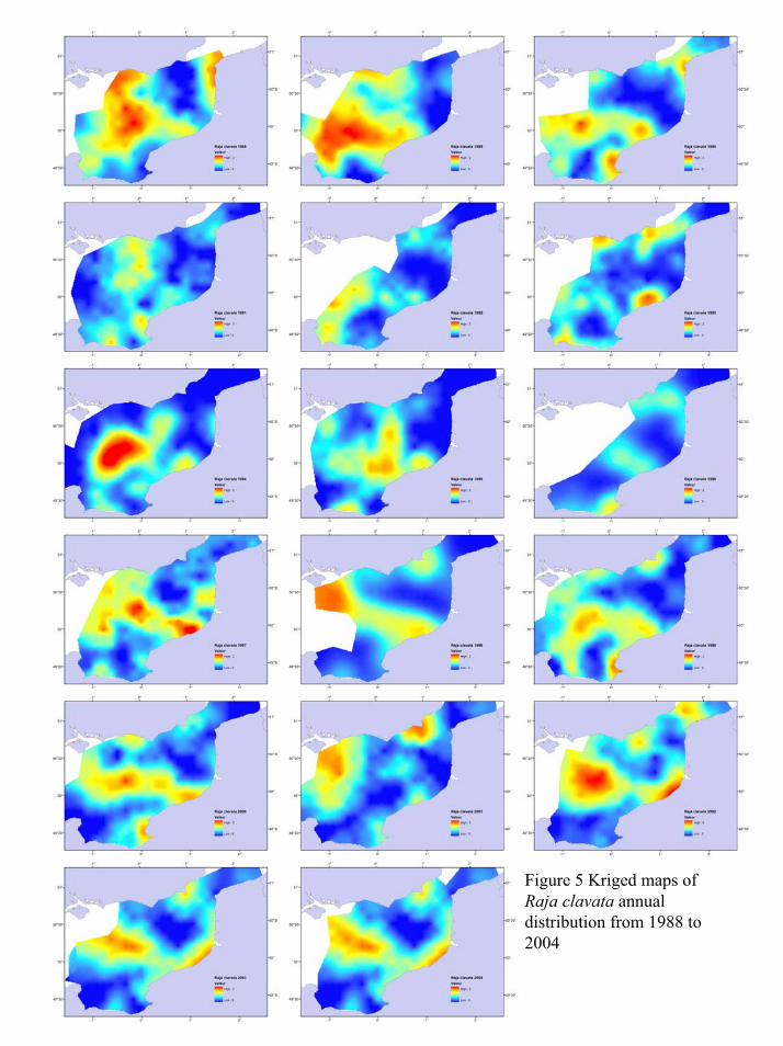
Figure 5 Kriged maps of Raja clavata annual distribution from 1988 to 2004

Figure 6 Kriged maps of Scyliorhinus caniculaannual distribution from 1988 to 2004